Secure Control under Partial Observability with Temporal Logic Constraints^∗

Abstract

This paper studies the synthesis of control policies for an agent that has to satisfy a temporal logic specification in a partially observable environment, in the presence of an adversary. The interaction of the agent (defender) with the adversary is modeled as a partially observable stochastic game. The search for policies is limited to over the space of finite state controllers, which leads to a tractable approach to determine policies. The goal is to generate a defender policy to maximize satisfaction of a given temporal logic specification under any adversary policy. We relate the satisfaction of the specification in terms of reaching (a subset of) recurrent states of a Markov chain. We then present a procedure to determine a set of defender and adversary finite state controllers of given sizes that will satisfy the temporal logic specification. We illustrate our approach with an example.

I Introduction

Cyber-physical systems (CPSs) are complex entities in which the working of a physical system is governed by interactions with computing devices and algorithms. These systems are ubiquitous [1], and vary in scale from power systems to medical devices and robots. In applications like self-driving cars and robotics, the systems are expected to work in dynamically changing and potentially dangerous environments with a large degree of autonomy. A natural question to ask before solving a problem in this domain is the means by which the environment, goals, and constraints, if any, are specified.

Markov decision processes (MDPs) [2, 3] have been used to model environments where outcomes depend on both, an inherent randomness in the model (transition probabilities), and an action taken by an agent. These models have been extensively used in applications, including in robotics [4] and unmanned aircrafts [5]. Formal methods [6] are a means to verify the behavior of complex models against a rich set of specifications [7]. Linear temporal logic (LTL) is a particularly well-understood framework to express properties like safety, liveness, and priority [8, 9]. These properties can then be verified using off-the-shelf model solvers [10, 11].

The system might be the target of malicious attacks with the aim of preventing it from reaching a goal. An attack can be carried out on the physical system, on the computers that control the working of the system, or on communication channels between components of the system. Such attacks have been reported across multiple application domains like power systems [12], automobiles [13], water networks [14], and nuclear reactors [15]. Therefore, strategies that are designed to only address modeling and sensing errors and uncertainties may not be optimal in the presence of an intelligent adversary who can manipulate the operation of the system.

Prior work in verifying the satisfaction of an LTL formula over an MDP or a stochastic game assumes that the states are fully observable. In many practical scenarios, this may not be the case. For example, a robot might only have an estimate of its current location based on the output of a vision sensor [16]. This necessitates the use of a framework that accounts for partial observability. For the single-agent case, partially-observable Markov decision processes (POMDPs) can be used to try and solve the problem. However, partial observability is a serious limitation in determining an ‘optimal policy’ for an agent. This demonstrates the need for techniques to determine approximate solutions. Heuristics to approximately solve POMDPs include belief replanning, most likely belief state policy, and entropy weighting [17], [18], grid-based methods [19], and point-based methods [20].

A large body of work studies classes of problems that are relevant to this paper (see Sec VI). These can be divided into three broad categories: i): synthesis of strategies for systems represented as an MDP that has to additionally satisfy a TL formula; ii): synthesis of strategies for POMDPs; iii): synthesis of defender and adversary strategies for an MDP under a TL constraint. While there has been recent work on the synthesis of controllers for POMDPs under TL specifications, these have largely been restricted to the single-agent case, and do not address the case when there might be an adversary with a competing objective.

In this paper, we study the problem of determining strategies for an agent that has to satisfy an LTL formula in the presence of an adversary in a partially observable environment. The defender and adversary take actions simultaneously, and these jointly influence the transitions of the system. Our approach is motivated by the treatment in [21] and [22] which propose the synthesis of parameterized finite state controllers (FSCs) for a POMDP that will maximize the probability of satisfaction of an LTL formula. This is an approximate strategy since it refrains from using the entire observation and action histories and uses only the most recent observation in order to determine an action. Although this restricts the class of policies that are searched over, FSCs are attractive since they can be used to solve the average reward problem over the infinite horizon [22].

I-A Contributions

We extend this setting to include an adversary who is also limited in that it does not exactly observe the state. The adversary policy is determined by an FSC, whose goal is opposite to that of the defender. The goal for the defender will be to synthesize a policy that will maximize satisfaction of an LTL formula for any adversary policy. We show that this is equivalent to maximizing, under any adversary policy, the probability of reaching a recurrent set of a Markov chain that additionally contains states that need to be reached in order to satisfy the LTL formula. The search for policies involve optimizing over both the size of the FSC and its parameters (transition probabilities). We present a procedure that will allow for the determining of defender and adversary FSCs of fixed sizes that will satisfy the LTL formula with nonzero probability. The search for a defender policy that will maximize the probability of satisfaction of the LTL formula for any adversary policy is then reduced to a search among these FSCs of fixed size. If these FSCs are parameterized in an appropriate way, it might lend itself to gradient-based optimization techniques.

I-B Outline

A quick introduction to LTL and partially observable stochastic games (POSGs) is given in Section II. We set up our problem in Section III, where we first define FSCs for the two agents, and show how they can be composed with a POSG to yield a Markov chain. Section IV presents our main results relating LTL satisfaction on a POSG to reaching recurrent sets of a Markov chain, and a procedure to determine candidate FSCs. An illustrative example is presented in Section V. Section VI summarizes related work in POMDPs and TL satisfaction on MDPs, and Section VII concludes the paper, along with a pointer to future directions of research.

II Preliminaries

In this section, we give a concise introduction to linear temporal logic and partially observable stochastic games. We then detail the construction of an entity which will ensure that runs on a POSG will satisfy an LTL formula.

II-A Linear Temporal Logic

A linear temporal logic (LTL) formula [6] is defined over a set of atomic propositions $\mathcal{AP}$, and can be inductively written as: $\phi:=\mathtt{T}|\sigma|\neg\phi|\phi\wedge\phi|\mathbf{X}\phi|\phi\mathbf{U}\phi$

Here, $\sigma\in\mathcal{AP}$, and $\mathbf{X}$ and $\mathbf{U}$ are temporal operators denoting the next and until operations respectively.

The semantics of LTL are defined over (infinite) words in $2^{\mathcal{AP}}$, and we write $\eta_{0}\eta_{1}\dots:=\eta\models\phi$ when a trace $\eta\in(2^{\mathcal{AP}})^{\omega}$ satisfies an LTL formula $\phi$. Further, let $\eta^{i}=\eta_{i}\eta_{i+1}\dots$. Then, $\eta\models\mathtt{T}$ if and only if (iff) $\eta_{0}$ is true; $\eta\models\sigma$ iff $\sigma\in\eta_{0}$; $\eta\models\neg\phi$ iff $\eta\not\models\phi$; $\eta\models\phi_{1}\wedge\phi_{2}$ iff $\eta\models\phi_{1}$ and $\eta\models\phi_{2}$; $\eta\models\mathbf{X}\phi$ iff $\eta^{1}\models\phi$; $\eta\models\phi_{1}\mathbf{U}\phi_{2}$ iff $\exists j\geq 0$ such that $\eta^{j}\models\phi_{2}$ and for all $k<j,\eta^{k}\models\phi_{1}$.

Further, the logic admits derived formulas of the form: i): $\phi_{1}\vee\phi_{2}:=\neg(\neg\phi_{1}\wedge\neg\phi_{2})$; ii): $\phi_{1}\Rightarrow\phi_{2}:=\neg\phi_{1}\vee\phi_{2}$; iii): $\mathbf{F}\phi:=\mathtt{T}\mathbf{U}\phi\text{ (eventually)}$; iv): $\mathbf{G}\phi:=\neg\mathbf{F}\neg\phi\text{ (always)}$.

Definition II.1

A deterministic Rabin automaton (DRA) is a quintuple $\mathcal{RA}=(Q,\Sigma,\delta,q_{0},F)$ where $Q$ is a nonempty finite set of states, $\Sigma$ is a finite alphabet, $\delta:Q\times\Sigma\rightarrow Q$ is a transition function, $q_{0}\in Q$ is the initial state, and $F:=\{(L(i),K(i)\}_{i=1}^{M}$ is such that $L(i),K(i)\subseteq Q$ for all $i$, and $M$ is a positive integer.

A run of $\mathcal{RA}$ is an infinite sequence of states $q_{0}q_{1}\dots$ such that $q_{i}\in\delta(q_{i-1},\alpha)$ for all $i$ and for some $\alpha\in\Sigma$. The run is accepting if there exists $(L,K)\in F$ such that the run intersects with $L$ finitely many times, and with $K$ infinitely often. An LTL formula $\phi$ over $\mathcal{AP}$ can be represented by a DRA with alphabet $2^{\mathcal{AP}}$ that accepts all and only those runs that satisfy $\phi$.

II-B Partially Observable Stochastic Games

Definition II.2

A stochastic game [23] is a tuple $\mathcal{G}:=(S,U_{def},U_{adv},\mathbb{T},\mathcal{AP},\mathcal{L})$. $S$ is a finite set of states, $s_{0}\in S$ is the initial state, $U_{def}$ and $U_{adv}$ are the finite sets of actions of the defender and adversary. $\mathbb{T}:S\times U_{def}\times U_{adv}\times S\rightarrow[0,1]$ encodes $\mathbb{T}(s^{\prime}|s,u_{def},u_{adv})$, the probability of transition from a state $s$ to a state $s^{\prime}$ when defender and adversary actions are $u_{def}$ and $u_{adv}$ respectively. $\mathcal{AP}$ is a set of atomic propositions, and $\mathcal{L}:S\rightarrow 2^{\mathcal{AP}}$ is a labeling function that maps a state to a subset of atomic propositions that are satisfied in that state.

A stochastic game can thus be viewed as an extension of Markov decision processes (MDPs) to the case when there is more than one player taking an action.

When $U_{adv}=\emptyset$ and $|U_{def}|=1$, $\mathcal{G}$ is a Markov chain (MC). For $s,s^{\prime}\in S$, $s^{\prime}$ is accessible from $s$, written $s\rightarrow s^{\prime}$, if $\mathbb{T}(s_{a}|s)\mathbb{T}(s_{b}|s_{a})\dots\mathbb{T}(s_{i}|s_{j})\mathbb{T}(s^{\prime}|s_{i})>0$ for some (finite subset of) states $s_{a},s_{b},\dots,s_{i},s_{j}$. Equivalently, $s\rightarrow s^{\prime}$ if there is a positive probability of reaching $s^{\prime}$ from $s$ in a finite number of steps. Two states communicate, written $s\leftrightarrow s^{\prime}$, if $s\rightarrow s^{\prime}$ and $s^{\prime}\rightarrow s$. Communicating classes of states cover the state space of the MC. A state is transient if there is a nonzero probability of not returning to it when we start from that state, and is positive recurrent otherwise. If some state in a communicating class is recurrent (transient), then the same holds for all other states in that class. Moreover, in a finite state MC, every state is either transient or positive recurrent. We refer the reader to [24] for a detailed exposition.

Partially observable stochastic games (POSGs) extend Definition II.2 to the case when states may not be observable, and each agent could observe the state according to a different observation function. This can be viewed as an interpretation of POMDPs to the case when there is more than one player.

Definition II.3

A partially observable stochastic game
is $\mathcal{SG}:=(S,U_{def},U_{adv},\mathbb{T},\mathcal{O}_{def},\mathcal{O}_{adv},O_{def},O_{adv},\mathcal{AP},\mathcal{L})$, where $S,U_{def},U_{adv},\mathbb{T},\mathcal{AP},\mathcal{L}$ are as in Definition II.2. $\mathcal{O}_{def},\mathcal{O}_{adv}$ denote the (finite) sets of observations available to the defender and adversary. $O_{*}:S\times\mathcal{O}_{*}\rightarrow[0,1]$ encodes $\mathbb{P}(o_{*}|s)$, where $*\in\{def,adv\}$.

The functions $O_{*}$ can be viewed as a means to model imperfect sensing. Then, we have $\sum_{o\in\mathcal{O}_{*}}O_{*}(o|s)=1$.

The information available until time $t$, denoted $\mathfrak{I}_{t}$, can be inductively defined as: $\mathfrak{I}_{0}=S$, $\mathfrak{I}_{t}=\mathfrak{I}_{t-1}\times U_{def}\times\mathcal{O}_{def}\times U_{adv}\times\mathcal{O}_{adv}$. The overall information is $\mathfrak{I}:=\cup_{t}\mathfrak{I}_{t}$.

Definition II.4

A (defender or adversary) policy for the POSG is a map from the overall information to a probability distribution over the respective action space, i.e. $\mu_{*}:\mathfrak{I}\times U_{*}\rightarrow[0,1]$, where $*\in\{def,adv\}$.

Policies of the form above are called randomized policies. If $\mu_{*}:\mathfrak{I}\rightarrow U_{*}$, it is called a deterministic policy.

In this paper, defender and adversary policies will be determined by probability distributions over transitions in finite state controllers (Sec III-A) that are composed with the POSG. This method is chosen because the FSCs when composed with the product-POSG (Sec II-C), will result in a finite state Markov chain.

II-C The Product-POSG

In order to find runs on $\mathcal{SG}$ that would be accepted by a DRA $\mathcal{RA}$ built from an LTL formula $\phi$, we construct a product-POSG. This construction is motivated by the product-stochastic game construction in [23] and the product-POMDP construction in [21].

Definition II.5

Given a POSG $\mathcal{SG}$ and a DRA $\mathcal{RA}$ corresponding to an LTL formula $\phi$, a product-POSG is a tuple $\mathcal{SG}^{\phi}=(S^{\phi},U_{def},U_{adv},\mathbb{T}^{\phi},\mathcal{O}_{def},\mathcal{O}_{adv},O_{def}^{\phi},O_{adv}^{\phi},F^{\phi},\mathcal{AP},\mathcal{L}^{\phi})$.

Here, $S^{\phi}=S\times Q$, $\mathbb{T}^{\phi}((s^{\prime},q^{\prime})|(s,q),u_{def},u_{adv})=\mathbb{T}(s^{\prime}|s,u_{def},u_{adv})$ iff $\delta(q,\mathcal{L}(s^{\prime}))=q^{\prime}$, and $0$ otherwise, $O_{*}^{\phi}(o|(s,q))=O_{*}(o|s)$, $F^{\phi}=\{(L^{\phi}(i),K^{\phi}(i))\}_{i=1}^{M}$ with $L^{\phi}(i),K^{\phi}(i)\subset S^{\phi}$, and $(s,q)\in L^{\phi}(i)$ iff $q\in L(i)$, $(s,q)\in K^{\phi}(i)$ iff $q\in K(i)$, $\mathcal{L}^{\phi}((s,q))=\mathcal{L}(s)$.

From the above definition, it is clear that acceptance conditions in the product-POSG depend on the DRA while the transition probabilities of the product-POSG are determined by transition probabilities of the original POSG. Therefore, a run on the product-POSG can be used to generate a path on the POSG and a run on the DRA. Then, if the run on the DRA is accepting, we say that the product-POSG satisfies the LTL specification $\phi$.

III Problem Setup

This section details the construction of finite state controllers (FSCs) for the defender and adversary. An FSC for an agent can be interpreted as a policy for that agent. When the FSCs are composed with the product-POSG, the resulting entity is a Markov chain. We then establish a way to determine satisfaction of an LTL specification on the product-POSG in terms of runs on the composed Markov chain. A treatment for the single-agent case when the environment is specified as a POMDP was presented in [21].

$$\mathbb{T}^{\phi,\mathcal{C}_{def},\mathcal{C}_{adv}}((s^{\prime},q^{\prime}),g^{\prime}_{def},g^{\prime}_{adv}|(s,q),g_{def},g_{adv})$$ (1)

$$=\sum_{o\in\mathcal{O}_{def}}\sum_{o^{\prime}\in\mathcal{O}_{adv}}\sum_{u_{def}}\sum_{u_{adv}}O_{def}(o|s)O_{adv}(o^{\prime}|s)\mu_{def}(g^{\prime}_{def},u_{def}|g_{def},o)\mu_{adv}(g^{\prime}_{adv},u_{adv}|g_{adv},o^{\prime})\mathbb{T}^{\phi}((s^{\prime},q^{\prime})|(s,q),u_{def},u_{adv})$$

$$O_{def}(o_{def}|s)O_{adv}(o_{adv}|s)\mu_{def}(g^{\prime}_{def},u_{def}|g_{def},o_{def})\mu_{adv}(g^{\prime}_{adv},u_{adv}|g_{adv},o_{adv})\mathbb{T}^{\phi}((s^{\prime},q^{\prime})|(s,q),u_{def},u_{adv})>0$$ (2)

$$O_{def}(o_{def}|s)O_{adv}(o_{adv}|s)\mu_{def}(g^{\prime\prime}_{def},u_{def}|g_{def},o_{def})\mu_{adv}(g^{\prime\prime}_{adv},u_{adv}|g_{adv},o_{adv})\mathbb{T}^{\phi}((s^{\prime\prime},q^{\prime\prime})|(s,q),u_{def},u_{adv})>0$$ (3)

III-A Finite State Controllers

Finite state controllers comprise a finite set of internal states. The transitions between any two states is governed by the current observation of the agent. A directed cyclic graph of internal states of the FSC will allow for remembering events relevant to taking optimal actions [21]. In our setting, we will have two FSCs, one for the defender and another for the adversary. We will then limit the search for defender and adversary policies to one over FSCs of fixed cardinality.

Definition III.1

A finite state controller for the defender (adversary), denoted $\mathcal{C}_{def}$ ($\mathcal{C}_{adv}$) is a tuple $\mathcal{C}_{*}=(G_{*},\mu_{*})$, where $G_{*}$ is a finite set of (internal) states of the controller, $\mu_{*}:G_{*}\times\mathcal{O}_{*}\times G_{*}\times U_{*}\rightarrow[0,1]$, written $\mu_{*}(g^{\prime}_{*},u_{*}|g_{*},o_{*})$, is a probability distribution of the next internal state and action, given a current internal state and observation. The initial state of $\mathcal{C}_{*}$ is a probability distribution over $G_{*}$, and will depend on the initial state of the system. Here, $*\in\{def,adv\}$.

The setup works as follows: Initial states of the FSCs are determined by the initial state of the POSG. At each time step, the defender will observe the state of $\mathcal{SG}^{\phi}$ according to $O_{def}$ and will commit to a policy $\mu_{def}(\cdot)$ generated by $\mathcal{C}_{def}$. The adversary observes this and the state according to $O_{adv}$ and responds with $\mu_{adv}(\cdot)$ generated by $\mathcal{C}_{adv}$. These actions are taken concurrently, and are applied to $\mathcal{SG}^{\phi}$, which transitions to the next state per the distribution $\mathbb{T}^{\phi}(\cdot)$, and the process is repeated.

Definition III.2

An FSC is proper if there is a positive probability of satisfying a given LTL formula in a finite number of steps under this policy on a system represented by a POMDP.

This is similar to the definition in [25], with the distinction that the terminal state of an FSC in that context will be directly related to Rabin acceptance pairs of a Markov chain formed by composing $\mathcal{C}_{def}$ and $\mathcal{C}_{adv}$ with a product-POSG (Sec III-B). We will restrict ourselves to proper FSCs for the rest of this paper.

III-B The Global Markov Chain

The FSCs $\mathcal{C}_{def}$ and $\mathcal{C}_{adv}$, when composed with $\mathcal{SG}^{\phi}$, will result in a finite-state, fully observable Markov chain. To maintain consistency with the literature, we will refer to this as the global Markov chain (GMC) [21].

Definition III.3

The global Markov chain resulting from a product-POSG $\mathcal{SG}^{\phi}$ controlled by FSCs $\mathcal{C}_{def}$ and $\mathcal{C}_{adv}$ is the tuple $\mathcal{M}:=\mathcal{M}^{\phi,\mathcal{C}_{def},\mathcal{C}_{adv}}=(S^{\phi,\mathcal{C}_{def},\mathcal{C}_{adv}},\mathbb{T}^{\phi,\mathcal{C}_{def},\mathcal{C}_{adv}},\mathcal{AP},\mathcal{L}^{\phi,\mathcal{C}_{def},\mathcal{C}_{adv}})$, where $S^{\phi,\mathcal{C}_{def},\mathcal{C}_{adv}}=S^{\phi}\times G_{def}\times G_{adv}$, $\mathcal{L}^{\phi,\mathcal{C}_{def},\mathcal{C}_{adv}}((s,q),g_{def},g_{adv})=\mathcal{L}^{\phi}((s,q))$, and $\mathbb{T}^{\phi,\mathcal{C}_{def},\mathcal{C}_{adv}}$ is given by Equation (1).

Similar to $\mathcal{SG}^{\phi}$, the Rabin acceptance condition for $\mathcal{M}$ is: $F^{\phi,\mathcal{C}_{def},\mathcal{C}_{adv}}=\{(L^{\phi,\mathcal{C}_{def},\mathcal{C}_{adv}}(i),K^{\phi,\mathcal{C}_{def},\mathcal{C}_{adv}}(i))\}_{i=1}^{M}$, with $(s,q,g_{def},g_{adv})\in L^{\phi,\mathcal{C}_{def},\mathcal{C}_{adv}}(i)$ iff $(s,q)\in L^{\phi}(i)$ and $(s,q,g_{def},g_{adv})\in K^{\phi,\mathcal{C}_{def},\mathcal{C}_{adv}}(i)$ iff $(s,q)\in K^{\phi}(i)$.

A state of $\mathcal{M}$ is of the form $\mathfrak{s}=(s,q,g_{def},g_{adv})$. A path on $\mathcal{M}$ is a sequence $\pi:=\mathfrak{s}_{0}\mathfrak{s}_{1}\dots$ such that $\mathbb{T}(\mathfrak{s}_{k+1}|\mathfrak{s}_{k})>0$, where $\mathbb{T}(\cdot)$ here corresponds to the transition probabilities in $\mathcal{M}$. A path on $\mathcal{M}$ is accepting if it satisfies the Rabin acceptance condition. This corresponds to an execution in $\mathcal{SG}^{\phi}$ controlled by $\mathcal{C}_{def}$ and $\mathcal{C}_{adv}$. A probability space over $\mathcal{M}$ is defined in the usual way [6].

III-C System Model

Consider a discrete-time finite-state system: $x(t+1)=f(x(t),u_{def}(t),u_{adv}(t),\mathtt{v}(t))$, where $\mathtt{v}(t)$ represents a stochastic disturbance. This system can be abstracted as an SG with finite state and action spaces using a simulation-based algorithm, similar to that in [26].

III-D Problem Statement

The goal is to synthesize a defender policy that will maximize the probability of satisfaction of an LTL specification under any adversary policy. Clearly, this will depend on the FSCs, $\mathcal{C}_{def}$ and $\mathcal{C}_{adv}$. In this paper, we will assume that the size of the adversary FSC is fixed, and known. This can be interpreted as one way for the defender to have knowledge of the capabilities of an adversary, which is a reasonable assumption. Future work will consider the problem for FSCs of arbitrary sizes. Formally,

Problem III.4

Given a partially observable environment and an LTL formula, determine a defender policy specified by a finite state controller that maximizes the probability of satisfying the LTL formula under any adversary policy that is represented as a finite state controller of fixed size $|G_{adv}|=G_{A}$. That is,

$$\max_{\mathcal{C}_{def}}\min_{\mathcal{C}_{adv}}\mathbb{P}(\mathcal{SG}^{\phi}\models\phi|\mathcal{C}_{def},\mathcal{C}_{adv},|G_{adv}|=G_{A})$$ (4)

Optimizing over $\mathcal{C}_{def}$ and $\mathcal{C}_{adv}$ indicates that the solution will depend on $|G_{def}|$, $\mu_{def}(\cdot)$, and $\mu_{adv}(\cdot)$.

IV Results

IV-A LTL Satisfaction and Recurrent Sets

Our main result relates the probability of the LTL specification being satisfied by the product-POSG, denoted $\mathcal{SG}^{\phi}\models\phi$, in terms of recurrent sets of the GMC. Let $\mathcal{R}:=\mathcal{R}^{\phi,\mathcal{C}_{def},\mathcal{C}_{adv}}$ denote the recurrent states of $\mathcal{M}$ under FSCs $\mathcal{C}_{def}$ and $\mathcal{C}_{adv}$. Let $\mathcal{R}^{S}:=(s,q)$ be the restriction of a recurrent state to a state of $\mathcal{SG}^{\phi}$.

Proposition IV.1

$\mathbb{P}(\mathcal{SG}^{\phi}\models\phi)>0$ if and only if there exists $\mathcal{C}_{def}$ such that for any $\mathcal{C}_{adv}$, there exists a Rabin acceptance pair $(L^{\phi}(i),K^{\phi}(i))$ and an initial state of $\mathcal{M}$, $m_{0}$, the following conditions hold:

$$K^{\phi}(i)\cap\mathcal{R}^{S}\neq\emptyset$$

$$m_{0} \rightarrow(K^{\phi}(i)\times G_{def}\times G_{adv})\cap\mathcal{R}$$ (5)

$$m_{0} \centernot\rightarrow(L^{\phi}(i)\times G_{def}\times G_{adv})\cap\mathcal{R}$$

Proof:

If for every $(L^{\phi}(i),K^{\phi}(i))$, at least one of the conditions in Equation (5) does not hold, then at least one of the following statements is true: i): no state that has to be visited infinitely often is recurrent; ii): there is no initial state from which a recurrent state that has to be visited infinitely often is accessible; iii): some state that has to be visited only finitely often in steady state is recurrent. This means $\mathcal{SG}^{\phi}\not\models\phi$ for all $\mathcal{C}_{def}$.

Conversely, if all the conditions in Equation (5) hold for some $(L^{\phi}(i),K^{\phi}(i))$, then $\mathcal{SG}^{\phi}\models\phi$ by construction. ∎

To quantify the satisfaction probability for a defender policy under any adversary policy, assume that the recurrent states of $\mathcal{M}$ are partitioned into recurrence classes $\{R_{1},\dots,R_{p}\}$. This partition is maximal, in the sense that two recurrent classes cannot be combined to form a larger recurrent class, and all states within a given recurrent class communicate with each other [22].

Definition IV.2

A recurrent set $R_{k}$ is $\phi-$feasible under FSCs $\mathcal{C}_{def}$ and $\mathcal{C}_{adv}$ if there exists $(L^{\phi}(i),K^{\phi}(i))$ such that $K^{\phi}(i)\cap R^{S}_{k}\neq\emptyset$ and $L^{\phi}(i)\cap R^{S}_{k}=\emptyset$. Let $\phi-RecSets^{\mathcal{C}_{def},\mathcal{C}_{adv}}$ denote the set of $\phi-$feasible recurrent sets under the respective FSCs.

Over infinite executions, a path of $\mathcal{M}$ will reach a recurrent set. Let $\pi\rightarrow R$ denote the event that such a path will reach a recurrent set. Then, Theorem IV.3 states that Problem III.4 is equivalent to determining defender FSCs that maximize the probability of reaching $\phi-$feasible recurrent sets of the GMC under any adversary FSC.

Theorem IV.3

$$\max_{\mathcal{C}_{def}}\min_{\mathcal{C}_{adv}}\mathbb{P}(\mathcal{SG}^{\phi}\models\phi|\mathcal{C}_{def},\mathcal{C}_{adv})$$

$$=\max_{\mathcal{C}_{def}}\min_{\mathcal{C}_{adv}}\sum_{R\in\phi-RecSets^{\mathcal{C}_{def},\mathcal{C}_{adv}}}\mathbb{P}(\pi\rightarrow R)$$ (6)

Proof:

Since the recurrence classes are maximal, $\mathbb{P}(\pi\rightarrow(R_{1}\cup\dots\cup R_{p}))=\sum_{k=1}^{p}\mathbb{P}(\pi\rightarrow R_{k})$. From Definition IV.2, a $\phi-$feasible recurrent set will necessarily contain a Rabin acceptance pair. Therefore, the probability of $\mathcal{SG}^{\phi}$ satisfying the LTL formula under $\mathcal{C}_{def}$ and $\mathcal{C}_{adv}$ is equivalent to the probability of paths on $\mathcal{M}$ leading to $\phi-$feasible recurrent sets. That is, $\mathbb{P}(\mathcal{SG}^{\phi}\models\phi|\mathcal{C}_{def},\mathcal{C}_{adv})=\sum_{R\in\phi-RecSets^{\mathcal{C}_{def},\mathcal{C}_{adv}}}\mathbb{P}(\pi\rightarrow R)$.

Then, for some (fixed) $\mathcal{C}_{def}$ (and initial state $\mathfrak{s}$ of $\mathcal{M}$), the minimum probability of satisfying $\phi$ over all adversary FSCs is equal to the minimum probability of reaching a $\phi-$feasible recurrent set.

The result follows for a maximizing $\mathcal{C}_{def}$. ∎

Proposition IV.1 and Theorem IV.3 address a broader class of problems than in Problem III.4 since they do not assume that the size of the adversary FSC is fixed.

IV-B Determining Candidate $\mathcal{C}_{def}$ and $\mathcal{C}_{adv}$

If the sizes of $\mathcal{C}_{def}$ and $\mathcal{C}_{adv}$ are fixed, then their design is equivalent to determining the transition probabilities between their internal states. We are guided by the treatment in [22]. However, our framework differs in that we additionally consider the effect of the presence of an adversary while aiming to satisfy an LTL specification.

Let the FSC policies $\mu_{def}$ and $\mu_{adv}$ be parameterized by $\Phi_{def}$ and $\Phi_{adv}$ respectively. Then, with $*\in\{def,adv\}$, $\mu_{*}(g^{\prime}_{*},u_{*}|g_{*},o_{*}):=\mu_{*}(g^{\prime}_{*},u_{*}|g_{*},o_{*},\Phi_{*})$. Any parameterization of the controller is valid so long as it obeys the laws of probability. We use the softmax parameterization [22, 27], since it is convex and its derivative can be easily computed. Let $\phi_{g^{\prime}_{*},u_{*}|g_{*},o_{*}}\in\mathbb{R}$ determine the relative probability of making a transition in the FSC along with taking a corresponding action given an observation. Then, the transition probabilities of the FSCs are:

$$\mu_{*}(g^{\prime}_{*},u_{*}|g_{*},o_{*},\Phi)= \frac{e^{\phi_{g^{\prime}_{*},u_{*}|g_{*},o_{*}}}}{\sum_{g_{*}\in G_{*}}\sum_{u_{*}\in U_{*}}e^{\phi_{g^{\prime}_{*},u_{*}|g_{*},o_{*}}}}$$ (7)

The parameterization considered in Algorithm 1 can be viewed as a special case of the softmax parameterization with $\phi_{g^{\prime}_{*},u_{*}|g_{*},o_{*}}=0$ for all $g^{\prime}_{*},g_{*},o_{*},u_{*}$.

Define $\mathcal{I}_{*}:G_{*}\times\mathcal{O}_{*}\times G_{*}\times U_{*}\rightarrow\{0,1\}$, where $\mathcal{I}_{*}(g^{\prime},u|g,o)=1\Leftrightarrow\mu_{*}(g^{\prime},u|g,o)>0$. $\mathcal{I}_{*}(\cdot)$ then serves to indicate if it is possible for an observation $o$ in a state $g$ of an FSC to transition to $g^{\prime}$ in the FSC while issuing action $u$. We further assume that $\forall(g,o)\in G_{*}\times\mathcal{O}_{*},\exists(g^{\prime},u)\in G_{*}\times U_{*}$ such that $\mathcal{I}_{*}(g^{\prime},u|g,o)=1$ [22]. Let a state in the GMC be denoted $\mathfrak{s}:=(s,q,g_{def},g_{adv})$.

Algorithm 1 Generate candidate FSCs $\mathcal{C}_{def},\mathcal{C}_{adv}$

0:  $G_{def}$, $G_{adv}$, $\mathcal{SG}^{\phi}$, $\mathcal{I}_{def}^{o}$, $\mathcal{I}_{adv}^{o}$

0:  Set of admissible FSC structures $\mathbb{I}:=(\mathbb{I}_{def},\mathbb{I}_{adv})$, and transition probabilities, $(\mu_{def}(),\mu_{adv}())$ such that GMC has a $\phi-$feasible recurrent set

1:  Induce digraph $\mathcal{G}$ of $\mathcal{M}$ of $\mathbb{SG}^{\phi}$ under $\mathcal{I}_{def}^{o}$ and $\mathcal{I}_{adv}^{o}$ as $(\mathfrak{S},\mathcal{E})$, s.t. $\forall\mathfrak{s}_{1},\mathfrak{s}_{2}\in\mathfrak{S}:\mathfrak{s}_{1}\rightarrow\mathfrak{s}_{2}\in\mathcal{E}\Leftrightarrow\mathbb{T}(\mathfrak{s}_{2}|\mathfrak{s}_{1})>0$.

2:  $\mathbb{I}_{def}=\mathbb{I}_{adv}=\emptyset$

3:  $\mathcal{C}=SCCs(\mathcal{G})=\{C_{1},\dots,C_{N}\}$

4:  for $C\in\mathcal{C}$ and $(L^{\phi}(i),K^{\phi}(i))\in F^{\phi}$ do

5:     $Bad_{i}=\{\mathfrak{s}^{\prime}\notin C:\exists\mathfrak{s}\in C\text{ s.t. }\mathfrak{s}\rightarrow\mathfrak{s}^{\prime}\}$

6:     $Bad_{i}=Bad_{i}\cup(C\cap(L^{\phi}(i)\times G_{def}\times G_{adv}))$

7:     $Good_{i}=C\cap(K^{\phi}(i)\times G_{def}\times G_{adv})$

8:     Set $\mathcal{I}_{*}(g^{\prime}_{*},u_{*}|g_{*},o_{*})=1$ for all $g^{\prime}_{*},g_{*},u_{*},o_{*}$

9:     while $\sum_{g^{\prime}_{*},u_{*}}\mathcal{I}_{*}(g^{\prime}_{*},u_{*}|g_{*},o_{*})>0\forall o_{*},g_{*}$ and $Bad_{i}\neq\emptyset$ do

10:        Choose $\mathfrak{s^{\prime}}=(s^{\prime},q^{\prime},g_{def}^{\prime},g_{adv}^{\prime})\in Bad_{i}$, $\mathfrak{s}^{\prime\prime}=(s^{\prime\prime},q^{\prime\prime},g_{def}^{\prime\prime},g_{adv}^{\prime\prime})\in Good_{i}$

11:        for $\mathfrak{s}=(s,q,g_{def},g_{adv})\in C\setminus Bad_{i}$ do

12:           for $u_{def}\in U_{def}$ do

13:              $\mu_{*}(g^{\prime}_{*},u_{*}|\Phi_{*},g_{*},o_{*})=\frac{\mathcal{I}_{*}(g^{\prime}_{*},u_{*}|g_{*},o_{*})}{\sum_{g^{\prime}_{*},u_{*}}\mathcal{I}_{*}(g^{\prime}_{*},u_{*}|g_{*},o_{*})}$

14:              if $\exists u_{adv}\in U_{adv}$ Eqn (2) holds  then

15:                 $\mathcal{I}_{def}(g^{\prime}_{def},u_{def}|g_{def},o_{def})\leftarrow 0$ $\forall g^{\prime}_{def},g_{def}\in G_{def}$

16:              end if

17:           end for

18:           for $u_{adv}\in U_{adv}$ do

19:              $\mu_{*}(g^{\prime\prime}_{*},u_{*}|\Phi_{*},g_{*},o_{*})=\frac{\mathcal{I}_{*}(g^{\prime\prime}_{*},u_{*}|g_{*},o_{*})}{\sum_{g^{\prime\prime}_{*},u_{*}}\mathcal{I}_{*}(g^{\prime\prime}_{*},u_{*}|g_{*},o_{*})}$

20:              if $\forall u_{def}\in U_{def}$, Eqn (3) holds then

21:                 $\mathcal{I}_{adv}(g^{\prime\prime}_{adv},u_{adv}|g_{adv},o_{adv})\leftarrow 0$

22:              end if

23:           end for

24:        end for

25:        $Bad_{i}=Bad_{i}\setminus\{\mathfrak{s}^{\prime}\}$

26:     end while

27:     Compute transition probabilities and construct digraph $\mathcal{G}_{new}$ of GMC of $\mathcal{SG}^{\phi}$ under modified $\mathcal{I}_{def}$ and $\mathcal{I}_{adv}$

28:     $\mathcal{C}_{new}=SCCs(\mathcal{G}_{new})$

29:     if $\exists\mathfrak{s}\in Good_{i}\text{ s.t. }\mathfrak{s}$ is recurrent in $\mathcal{G}_{new}$ then

30:        $\mathbb{I}=(\mathbb{I}_{def}\cup\mathcal{I}_{def},\mathbb{I}_{adv}\cup\mathcal{I}_{adv})$

31:     end if

32:  end for

In Algorithm 1, for defender and adversary FSCs with fixed number of states, we determine candidate $\mathcal{C}_{def}$ and $\mathcal{C}_{adv}$ such that the resulting $\mathcal{M}$ will have a $\phi-$feasible recurrent set. We start with initial candidate structures $\mathcal{I}_{*}^{o}$ and induce the digraph of the resulting GMC (Line 1). This MC might not contain a $\phi-$feasible recurrent set. We first determine the set of communicating classes of the MC, which is equivalent to determining the strongly connected components (SCCs) of the induced digraph (Line 3). A communicating class of the MC will be recurrent if it is a sink SCC of the corresponding digraph. The states in $Bad_{i}$ are those in $C$ that are part of the Rabin accepting pair that has to be visited only finitely many times (and therefore, to be visited with very low probability in steady state) (Line 6). $Bad_{i}$ further contains states that can be transitioned to from some state in $C$. This is because once the system transitions out of $C$, it will not be able to return to it in order to satisfy the Rabin acceptance condition (Line 5) (and hence, $C$ will not be recurrent). $Good_{i}$ contains those states in $C$ that need to be visited infinitely often according to the Rabin acceptance condition (Line 7).

Recall that the agents have access to the actual state only via their individual observations. A defender action is forbidden if there exists an adversary action that will allow a transition to a state in $Bad_{i}$ under observations $o_{def}$ and $o_{adv}$. This is achieved by setting corresponding entries in $\mathcal{I}_{def}$ to zero (Lines 12-17). An adversary action is not useful if for every defender action, the probability of transitioning to a state in $Good_{i}$ is nonzero under $o_{def}$ and $o_{adv}$. This is achieved by setting the corresponding entry in $\mathcal{I}_{adv}$ to zero (Lines 18-23).

The computational complexity of Algorithm 1 depends on: i): determining the SCCs. This can be done in $\mathbf{O}(|\mathfrak{S}|+|\mathcal{E}|)$ [28]. We have $|\mathfrak{S}|=|S||G_{def}||G_{adv}|$ and $|\mathcal{E}|\leq|\mathfrak{S}|^{2}$. Therefore, the SCCs can be determined in $\mathbf{O}(|S|^{2}|G_{def}|^{2}|G_{adv}|^{2})$ in the worst case. ii): determining the structures in Lines 9-26. This, in the worst case, is $\mathbf{O}(|\mathfrak{S}|(|\mathcal{O}_{def}+|\mathcal{O}_{adv}|)(|\mathfrak{S}|(|U_{def}|+|U_{adv}|))$. Defining $|\mathcal{O}|=|\mathcal{O}_{def}|+|\mathcal{O}_{adv}|$ and $|U|=|U_{def}|+|U_{adv}|$, we have an overall computational complexity of $\mathbf{O}(|S|^{2}|G_{def}|^{2}|G_{adv}|^{2}|\mathcal{O}||U|)$.

Proposition IV.4

Algorithm 1 is sound. That is, each feasible FSC structure $(\mathcal{I}_{def},\mathcal{I}_{adv})$ in $\mathbb{I}$ will have at least one $\phi-$feasible recurrent set.

Proof:

This is by construction. The output of the algorithm is a set $\{\mathcal{I}_{def}^{i},\mathcal{I}_{adv}^{i}\}_{i=1}^{W}$ such that the resulting GMC for each case has a state that is recurrent and has to be visited infinitely often. This state, by Definition IV.2, belongs to $\phi-RecSet^{\mathcal{C}_{def}^{i},\mathcal{C}_{adv}^{i}}$. Moreover, if the algorithm returns a nonempty solution, a solution to Problem III.4 will exist since we assume that the FSCs are proper. ∎

Algorithm 1 is suboptimal since we only consider the most recent observations of the defender and adversary. It is also not complete, since there might be a feasible solution that cannot be determined by the algorithm.

Remark IV.5

For $\mathcal{C}_{def}$ and $\mathcal{C}_{adv}$ of fixed sizes and structures $\mathcal{I}_{def}$ and $\mathcal{I}_{adv}$, a solution to Problem III.4 is:

$$\max_{\Phi_{def}}\min_{\Phi_{adv}}\mathbb{P}(\mathcal{SG}^{\phi}\models\phi|\mathcal{C}_{def},\mathcal{C}_{adv})$$ (8)

This follows from the fact that for fixed FSC sizes and structures, the properties of a set (recurrent or transient) in the GMC will not change. What remains then is to choose the transition probabilities appropriately. For a softmax parameterization, this computation is presented in [22], and we omit it for want of space.

IV-C Determining Recurrent States to Visit

Algorithm 2 returns a subset of the recurrent states that are consistent with the Rabin acceptance pairs that need to be visited ‘often’ in steady state. If there is a reward structure over the states of the GMC that incentivizes visits to $Good_{k}$, then the expected long-term average reward is equal to the expected occupation measure of $Good_{k}$ [21]. Moreover, in the infinite horizon, we can assume that the system has been absorbed in a recurrent set, and the resulting (sub-)Markov chain is irreducible. Then, this problem can be solved by viewing it as minimizing an average cost per stage problem [2].

Algorithm 2 Recurrent states to visit in steady state

0:  $R_{k}\in\phi-RecSets^{FSC_{def},FSC_{adv}},\{L^{\phi}(i),K^{\phi}(i)\}_{i=1}^{M}$

0:  $Good_{k}\subseteq R_{k}$, the set of states that need to be visited ‘often’ in steady-state

1:  $Good_{k}=\emptyset$

2:  for $i=1$ to $M$ do

3:     if $((L^{\phi}(i)\times G_{def}\times G_{adv})\cap R_{k}=\emptyset)$ then

4:        $Good_{k}=Good_{k}\cup(((K^{\phi}(i)\times G_{def}\times G_{adv})\cap R_{k})$

5:     end if

6:  end for

V Example

Assume the state space is given by $S:=\{s_{i}:i=x+My,x\in\{0,\dots,M-1\},y\in\{0,\dots,N-1\}\}$. This will define an $M\times N$ grid. The defender’s actions are $U_{def}=\{R,L,U,D\}$ and the adversary’s actions are $U_{adv}=\{A,NA\}$, denoting right, left, up, down, attack, and not attack. The observations of both agents are $\mathcal{O}_{def}=\mathcal{O}_{adv}=\{correct,wrong\}$, with $O_{def}(correct|s_{i})=0.8=1-O_{def}(wrong|s_{i})$, and $O_{adv}(correct|s_{i})=0.6=1-O_{adv}(wrong|s_{i})$. Let $\mathcal{AP}=\{unsafe,goal\}$. Then, if $\phi=\mathbf{G}\mathbf{F}goal\wedge\mathbf{G}\neg unsafe$, it can be shown that the corresponding DRA will have two states $q_{0},q_{1}$, with $F=(\{\emptyset\},\{q_{1}\})$. The transition probabilities for $(u_{def},u_{adv})=(R,NA)$ and $(R,A)$ are defined below. The probabilities for other action pairs can be defined similarly. Let $N_{s_{i}}$ denote the neighbors of $s_{i}$.

$$\mathbb{T}(s_{j}|s_{i},R,NA)=\begin{cases}0.8&\text{$j=i+1$, $i+1\%M\neq 0$}\\ \frac{0.2}{|N_{s_{i}}|}&\text{($s_{j}\in\{s_{i}\}\cup N_{s_{i}}\setminus\{s_{i+1}\}$), $i+1\%M\neq 0$}\\ 1&\text{$j=i$ and $i+1\%M=0$}\\ \end{cases}$$

$$\mathbb{T}(s_{j}|s_{i},R,A)=\begin{cases}0.6&\text{$j=i+1$, $i+1\%M\neq 0$}\\ \frac{0.4}{|N_{s_{i}}|}&\text{($s_{j}\in\{s_{i}\}\cup N_{s_{i}}\setminus\{s_{i+1}\}$), $i+1\%M\neq 0$}\\ 1&\text{$j=i$ and $i+1\%M=0$}\end{cases}$$

For this example, let $M=3,N=2$. Then, $|S|=6$. Let $s_{4}$ be an unsafe state, and $s_{5}$ be the goal state. This is indicated in Figure 1. Let $|G_{def}|=2,|G_{adv}|=1$ for the FSCs. Assume that for some initial structures $\mathcal{I}_{def}^{0},\mathcal{I}_{adv}^{0}$ the GMC is given by Figure 1. The figure also indicates the states in terms of its individual components. Assume that the LTL formula $\phi$ is such that the states in green denote those that have to be visited infinitely often in steady state, while those in red must be avoided. Therefore $(L^{\phi},K^{\phi})=\{(\{\emptyset\},\{m_{1}\}),(\{m_{3}\},\{m_{2}\})\}$. The boxes $C_{1},C_{2},C_{3}$ indicate the communicating classes of the graph.

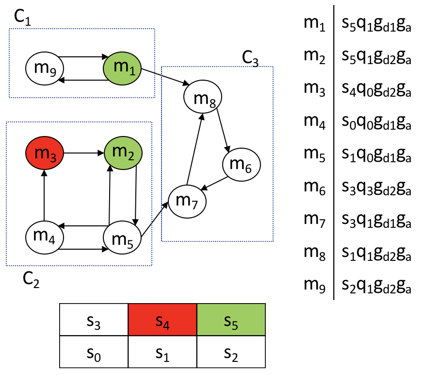
Figure 1: Clockwise, from top-left: Global Markov chain (GMC) for initial defender and adversary FSC structures- green states ($m_{1}\&m_{2}$) must be visited infinitely often, and state in red ($m_{3}$) must be visited finitely often in steady-state; GMC state $m_{i}\in S\times Q\times G_{def}\times G_{adv}$; State-space for $M=3,N=2$ showing unsafe ($s_{4}$) and target ($s_{5}$) states.

From Algorithm 1, for $C_{1}$, $Bad=\{m_{8}\},Good=\{m_{1}\}$. For $m_{1}\rightarrow m_{8}$, notice that Equation (2) is true for all $u_{adv}$ and $u_{def}=\{D,L\}$. Therefore, $\mathcal{I}_{def}(g^{\prime},u_{def}|g,o)\leftarrow 0$ for $o=\{correct,wrong\}$. For $m_{9}\rightarrow m_{1}$, since Equation (3) fails to hold for $R,D\in U_{def}$, $\mathcal{I}_{adv}(\cdot)$ remains unchanged. Then, $m_{1}$ is recurrent in $\mathcal{G}_{new}$. For $C_{2}$, $Bad=\{m_{3},m_{7}\},Good=\{m_{2}\}$. Like for $C_{1}$, $\mathcal{I}_{adv}(\cdot)$ remains unchanged, since Equation (3) does not hold for $D\in U_{def}$. Corresponding to $m_{5}\rightarrow m_{7}$, $\mathcal{I}_{def}(g^{\prime},u_{def}|g,o)\leftarrow 0\forall u_{def}\in U_{def}\setminus D$. A similar conclusion can be reached for $m_{4}\rightarrow m_{3}$. Then, $m_{2}$ will be recurrent in $\mathcal{G}_{new}$. For $C_{3}$, since $Bad=Good=\emptyset$, no structure is added to $\mathbb{I}$. Notice that these FSCs satisfy Proposition IV.1.

This example also demonstrates the limitations of Algorithm 1. From the $M\times N$ grid, it is clear there will exist a policy that takes the defender from any $s\in S\setminus\{s_{4}\}$ to $s_{5}$ with probability $1$. However, for FSCs of small size, the initial state of the defender might result in the Algorithm reporting that no solution was found, even if there exists a feasible solution.

VI Related Work

Satisfying TL constraints during motion planning for robots is an active area of research. Approaches include hierarchical control [29], ensuring probabilistic satisfaction guarantees [4], and sensing-based strategies [8].

The authors of [30] propose methods to synthesize a robust control policy that satisfies an LTL formula for a system represented as an MDP whose transitions are not exactly known, but are assumed to lie in a set. For MDPs under an LTL specification, a partial ordering on the states is leveraged to solve controller synthesis as a receding horizon problem in [31]. The synthesis of an optimal control policy that maximizes the probability of an MDP satisfying an LTL formula that additionally minimizes the cost between satisfying instances is studied in [9]. This is computed by determining maximal end components in an MDP. However, this approach will not work in the partially observable setting, where policies will depend on an observation of the state [32]. The synthesis of joint control and sensing strategies for discrete systems with incomplete information and sensing is presented in [33]. The setting of [9] in the additional presence of an adversary with competing objectives has been presented in [26].

A policy in a POSG (or POMDP), without loss of generality, depends on the ‘history’ of the system. That is, a policy at time $t$ depends on actions and observations at all previous times. A memoryless policy on the other hand, only depends on the current state. For fully observable stochastic games, it is possible to always find memoryless policies that are optimal. However, a policy with memory could perform much better than a memoryless policy for POSGs. One way of determining policies for a POSG is to keep track of the entire execution, observation, and action histories, which can be abstracted into determining a sufficient statistic for the POSG execution. One example is the belief state, which reflects the probability that the agent is in some state, based on receiving observations from the environment. Updating the belief state at every time step only requires knowledge of the previous belief state and the most recent action and observation. Thus, the belief states form the states of an MDP [34], which is more amenable to analysis [2] than a POMDP. However, the belief state is uncountable, and thus will not allow for the development of exact algorithms to determine strategies since these will require nontrivial and potentially infinite memory.

Synthesis of memoryless strategies for POMDPs in order to satisfy a specification was shown to be NP-hard and in PSPACE in [35]. In [36], a discretization of the belief space is carried out apriori, resulting in a fully observable MDP. However, this approach might not be practical if the state space is large [37]. The complexity of determining a winning strategy to solve the problem of determining the probability of satisfaction of parity objectives was shown to be undecidable in [38]. However, determining finite-memory strategies for the qualitative problem of parity objective satisfaction was shown to be EXPTIME-complete in [39].

Dynamic programming (DP) for POSGs has been studied in [40], resulting in an algorithm that generalizes both DP for POMDPs and iterated elimination of dominated strategies for normal form games. This work, however, considered the finite horizon case, and all agents had to maximize their own expected rewards. When agents cooperate to earn rewards, the framework is called a decentralized-POMDP (Dec-POMDP). The infinite horizon case for Dec-POMDPs was studied in [41], where the authors proposed a bounded policy iteration algorithm for policies represented as joint FSCs. A complete and optimal algorithm for deterministic FSC policies for DecPOMDPs was presented in [42]. Optimization techniques for ‘fixed-size controllers’ to solve Dec-POMDPs were investigated in [43]. A survey of recent research in Dec- POMDPs is presented in [44].

VII Conclusion

This paper presented, to the best of our knowledge, the first approach that uses finite state controllers to satisfy an LTL formula in a partially observable environment in the presence of an adversary. We showed that the probability of satisfaction of the LTL formula in this setting was equal to the probability of reaching recurrent classes of a Markov chain. Further, we presented a procedure to determine defender and adversary controllers of fixed sizes that result in a nonzero satisfaction probability of the LTL formula, and proved its soundness.

In ongoing and future work, we plan to investigate the case when the size of the defender FSC can be changed to improve the probability of satisfaction of the LTL formula. This has been done for the single agent case in [22], but extending it to an environment with an intelligent adversary will be challenging and interesting. We also plan to study applications of this framework.

References

- [1] R. Baheti and H. Gill, “Cyber-physical systems,” The Impact of Control Technology, vol. 12, no. 1, pp. 161–166, 2011.
- [2] D. P. Bertsekas, Dynamic Programming and Optimal Control 4th Edition, Volumes I and II. Athena Scientific, 2015.
- [3] M. L. Puterman, Markov decision processes: Discrete stochastic dynamic programming. John Wiley & Sons, 2014.
- [4] M. Lahijanian, S. B. Andersson, and C. Belta, “Temporal logic motion planning and control with probabilistic satisfaction guarantees,” IEEE Transactions on Robotics, vol. 28, no. 2, pp. 396–409, 2012.
- [5] S. Temizer, M. Kochenderfer, L. Kaelbling, T. Lozano-Pérez, and J. Kuchar, “Collision avoidance for unmanned aircraft using MDPs,” in AIAA Guidance, Navigation, and Control Conference, 2010.
- [6] C. Baier and J.-P. Katoen, Principles of model checking. MIT Press, 2008.
- [7] M. Lahijanian, S. B. Andersson, and C. Belta, “Formal verification and synthesis for discrete-time stochastic systems,” IEEE Transactions on Automatic Control, vol. 60, no. 8, pp. 2031–2045, 2015.
- [8] H. Kress-Gazit, G. E. Fainekos, and G. J. Pappas, “Where’s Waldo?: Sensor-based temporal logic motion planning,” in International Conference on Robotics and Automation. IEEE, 2007, pp. 3116–3121.
- [9] X. Ding, S. L. Smith, C. Belta, and D. Rus, “Optimal control of MDPs with linear temporal logic constraints,” IEEE Transactions on Automatic Control, vol. 59, no. 5, pp. 1244–1257, 2014.
- [10] A. Cimatti, E. Clarke, F. Giunchiglia, and M. Roveri, “Nusmv: A new symbolic model verifier,” in International Conference on Computer Aided Verification. Springer, 1999, pp. 495–499.
- [11] M. Kwiatkowska, G. Norman, and D. Parker, “Prism 4.0: Verification of probabilistic real-time systems,” in International Conference on Computer Aided Verification. Springer, 2011, pp. 585–591.
- [12] J. E. Sullivan and D. Kamensky, “How cyber-attacks in Ukraine show the vulnerability of the US power grid,” The Electricity Journal, vol. 30, no. 3, pp. 30–35, 2017.
- [13] Y. Shoukry, P. Martin, P. Tabuada, and M. Srivastava, “Non-invasive spoofing attacks for anti-lock braking systems,” in International Workshop on Cryptographic Hardware and Embedded Systems. Springer, 2013, pp. 55–72.
- [14] J. Slay and M. Miller, “Lessons learned from the Maroochy water breach,” in International Conference on Critical Infrastructure Protection. Springer, 2007, pp. 73–82.
- [15] J. P. Farwell and R. Rohozinski, “Stuxnet and the future of cyber war,” Survival, vol. 53, no. 1, pp. 23–40, 2011.
- [16] S. Thrun, W. Burgard, and D. Fox, Probabilistic robotics. MIT Press, 2005.
- [17] A. R. Cassandra, L. P. Kaelbling, and J. A. Kurien, “Acting under uncertainty: Discrete bayesian models for mobile-robot navigation,” in International Conference on Intelligent Robots and Systems, vol. 2. IEEE, 1996, pp. 963–972.
- [18] L. P. Kaelbling, M. L. Littman, and A. R. Cassandra, “Planning and acting in partially observable stochastic domains,” Artificial intelligence, vol. 101, no. 1-2, pp. 99–134, 1998.
- [19] R. I. Brafman, “A heuristic variable grid solution method for POMDPs,” in AAAI/IAAI, 1997, pp. 727–733.
- [20] H. Kurniawati, D. Hsu, and W. S. Lee, “SARSOP: Efficient point-based POMDP planning by approximating optimally reachable belief spaces.” in Robotics: Science and Systems, 2008.
- [21] R. Sharan and J. Burdick, “Finite state control of POMDPs with LTL specifications,” in Proceedings of the American Control Conference, 2014, pp. 501–508.
- [22] R. Sharan, “Formal methods for control synthesis in partially observed environments: Application to autonomous robotic manipulation,” Ph.D. dissertation, California Institute of Technology, 2014.
- [23] L. Niu and A. Clark, “Secure control under LTL constraints,” in Proceedings of the American Control Conference, 2018.
- [24] S. P. Meyn and R. L. Tweedie, Markov chains and stochastic stability. Springer Science & Business Media, 2012.
- [25] E. A. Hansen and R. Zhou, “Synthesis of hierarchical finite-state controllers for POMDPs.” in ICAPS, 2003, pp. 113–122.
- [26] L. Niu and A. Clark, “Optimal secure control with LTL constraints,” Under review.
- [27] D. Aberdeen, “Policy-gradient algorithms for POMDPs,” Ph.D. dissertation, The Australian National University, 2003.
- [28] R. Tarjan, “Depth-first search and linear graph algorithms,” SIAM Journal on Computing, vol. 1, no. 2, pp. 146–160, 1972.
- [29] G. E. Fainekos, A. Girard, H. Kress-Gazit, and G. J. Pappas, “Temporal logic motion planning for dynamic robots,” Automatica, vol. 45, no. 2, pp. 343–352, 2009.
- [30] E. M. Wolff, U. Topcu, and R. M. Murray, “Robust control of uncertain MDPs with LTL specifications,” in Proceedings of the Conference on Decision and Control. IEEE, 2012, pp. 3372–3379.
- [31] T. Wongpiromsarn, U. Topcu, and R. M. Murray, “Receding horizon temporal logic planning,” IEEE Transactions on Automatic Control, vol. 57, no. 11, pp. 2817–2830, 2012.
- [32] D. Sadigh, E. S. Kim, S. Coogan, S. S. Sastry, and S. A. Seshia, “A learning based approach to control synthesis of MDPs for LTL specifications,” in Proceedings of the Conference on Decision and Control. IEEE, 2014, pp. 1091–1096.
- [33] J. Fu and U. Topcu, “Synthesis of joint control and active sensing strategies under temporal logic constraints,” IEEE Transactions on Automatic Control, vol. 61, no. 11, pp. 3464–3476, 2016.
- [34] R. D. Smallwood and E. J. Sondik, “The optimal control of POMDPs over a finite horizon,” Operations Research, vol. 21, no. 5, pp. 1071–1088, 1973.
- [35] N. Vlassis, M. L. Littman, and D. Barber, “On the computational complexity of stochastic controller optimization in POMDPs,” ACM Transactions on Computation Theory, vol. 4, no. 4, 2012.
- [36] T. Wongpiromsarn and E. Frazzoli, “Control of probabilistic systems under dynamic, partially known environments with temporal logic specifications,” in Proceedings of the Conference on Decision and Control (CDC). IEEE, pp. 7644–7651.
- [37] H. Yu and D. P. Bertsekas, “On near optimality of the set of finite-state controllers for average cost POMDP,” Mathematics of Operations Research, vol. 33, no. 1, pp. 1–11, 2008.
- [38] K. Chatterjee, L. Doyen, and T. A. Henzinger, “A survey of partial-observation stochastic parity games,” Formal Methods in System Design, vol. 43, no. 2, pp. 268–284, 2013.
- [39] K. Chatterjee, L. Doyen, S. Nain, and M. Y. Vardi, “The complexity of partial-observation stochastic parity games with finite-memory strategies,” in International Conference on Foundations of Software Science and Computation Structures. Springer, 2014, pp. 242–257.
- [40] E. A. Hansen, D. S. Bernstein, and S. Zilberstein, “Dynamic programming for partially observable stochastic games,” in AAAI, vol. 4, 2004, pp. 709–715.
- [41] D. S. Bernstein, E. A. Hansen, and S. Zilberstein, “Bounded policy iteration for decentralized POMDPs,” in International Joint Conference on Artificial Intelligence, 2005, pp. 52–57.
- [42] D. Szer and F. Charpillet, “An optimal best-first search algorithm for solving infinite horizon DEC-POMDPs,” in European Conference on Machine Learning. Springer, 2005, pp. 389–399.
- [43] C. Amato, D. S. Bernstein, and S. Zilberstein, “Optimizing fixed-size stochastic controllers for POMDPs and decentralized POMDPs,” Autonomous Agents and Multi-Agent Systems, vol. 21, no. 3, pp. 293–320, 2010.
- [44] F. A. Oliehoek and C. Amato, A concise introduction to decentralized POMDPs. Springer, 2016.