Visual recognition in the wild by sampling deep similarity functions
Abstract
Recognising relevant objects or object states in its environment is a basic capability for an autonomous robot. The dominant approach to object recognition in images and range images is classification by supervised machine learning, nowadays mostly with deep convolutional neural networks (CNNs). This works well for target classes whose variability can be completely covered with training examples. However, a robot moving in the wild, i.e., in an environment that is not known at the time the recognition system is trained, will often face domain shift: the training data cannot be assumed to exhaustively cover all the within-class variability that will be encountered in the test data. In that situation, learning is in principle possible, since the training set does capture the defining properties, respectively dissimilarities, of the target classes. But directly training a CNN to predict class probabilities is prone to overfitting to irrelevant correlations between the class labels and the specific subset of the target class that is represented in the training set. We explore the idea to instead learn a Siamese CNN that acts as similarity function between pairs of training examples. Class predictions are then obtained by measuring the similarities between a new test instance and the training samples. We show that the CNN embedding correctly recovers the relative similarities to arbitrary class exemplars in the training set. And that therefore few, randomly picked training exemplars are sufficient to achieve good predictions, making the procedure efficient.
1 Introduction
Deep learning, and in particular convolutional neural networks, have revolutionised the field of visual recognition. However, the break-through has been achieved under the assumption of a stable domain, meaning that we have access to a sufficiently large training database that covers all the modes of variation of the target classes that we might encounter at test time. In practice, this is achieved either by operating in a constrained environment in which we can indeed exhaustively sample the expected visual variability; or by collecting and labeling very large datasets, in an attempt to brute-force the generalisation problem via a training set that exhaustively exposes the variability of the entire “visual world”. This procedure has enjoyed immense success for tasks where the class appearance is fairly static, and where finding data and labeling them is easy, if tedious (such as recognising cats in internet images, or cars in images taken by an autonomous vehicle). However, there are problems where it is not as easy to obtain ground truth that generalises to all relevant cases. For instance, some variations in the target class may be rare or access to them may be restricted. More importantly, there are situations where the target class undergoes domain shift, such that it is not only difficult, but impossible to know all admissible modes of variation in advance, and at test time we are bound to encounter examples which are not well represented in the training distribution. As a concrete example, imagine a robotic watchman that shall be shipped with the capability to recognise whether a door is open or closed (Fig. 1), in an a-priori unknown environment. The road-block for training a classifier is not that we cannot find enough images of doors. Rather, it is that new doors with different appearance are designed and built all the time.
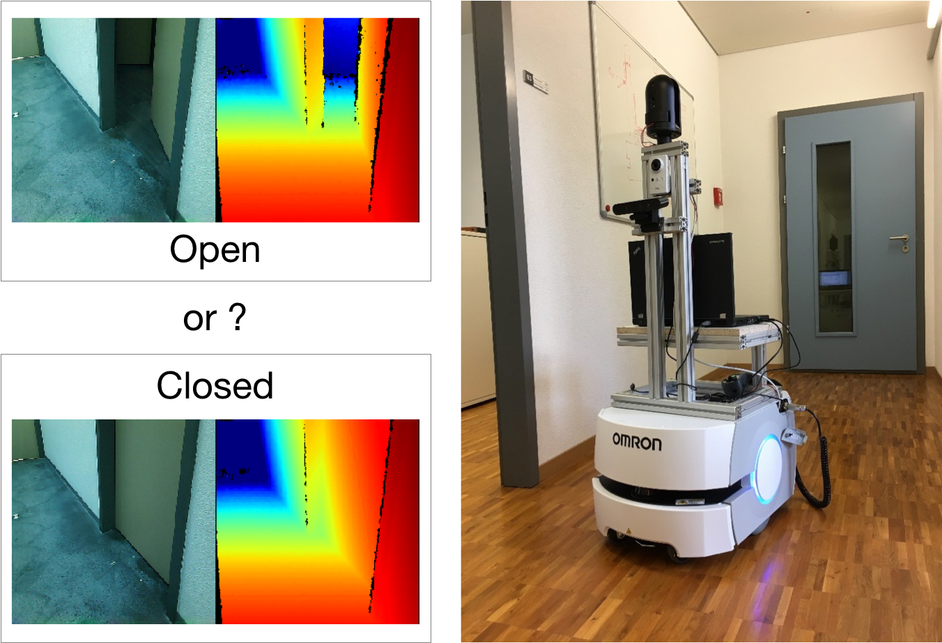
The problem is related to few-shot learning, although we are in the domain-shift scenario not adding a new, previously unseen class; in the sense that the relevant information to learn a suitable representation for the classification task is actually present in the data, but the learning is unable to separate important discriminative properties from irrelevant intra-class variation. Few-shot learning, say adding a new breed of dog to a classifier, aims to learn an embedding of the input images in which different classes form clusters, such that inter-class distances are higher than intra-class distances. The hope is that embedding a new class will lead to a new cluster, because the embedding generalises across different dog breeds, whereas a purely discriminative scheme could not be trained from only few examples. Classification with the learned distance function is achieved by computing distances between training and test examples, followed by nearest-neighbour classification.
We face a similar situation: pictures of open doors do have characteristic properties (like the bottom edge of the door not connecting the bottom ends of the frame). The problem is not that the crucial discriminative properties cannot be learned – they are captured in the training set. Rather, a straight-forward two-class CNN does not learn well enough to ignore legitimate intra-class variations not present in the training examples, i.e., it overfits to the training domain. Pre-training on a larger dataset and fine-tuning to the task-specific training dataset will possibly mitigate, but not solve the problem: there is no reason why pre-training on, say, ImageNet would inject exactly the information that is needed to generalise to the unseen doors (which are not observed in ImageNet, either). Likewise, heavier regularisation can potentially mitigate overfitting to biases in the training set, but empirically does not solve the problem – which is not that surprising: the regulariser favours similar outputs for nearby data points, but the domain shift is caused by examples that are far from all training samples, and thus calls for a notion of similarity that is valid everywhere on the input manifold.
We propose an approach based on a Siamese network for similarity learning. Our method is technically related to recent works on one-shot or few-shot deep learning [1, 2, 3, 4], but differs from them in one important aspect: few-shot learning aims to learn a new class from only few training examples (often motivated by the astonishing capabilities of biological vision), whereas we are concerned with generalisation of the same class beyond the domain covered by a (possibly not so small) training set. Computing similarities to all training examples for each test sample is computationally expensive. We show that it can be replaced by a random sampling procedure without performance penalty. In experiments on a diverse collection of datasets, our method consistently outperforms the direct classification baseline, reducing classification errors by 28-64%.
2 Related Work
Distance learning. In their comprehensive survey [5], Yang et al. classify distance learning methods into three groups, (i) unsupervised distance learning, (ii) supervised global distance learning, and (iii) supervised local distance learning. The idea of unsupervised methods is to learn a lower-dimensional embedding that preserves the pairwise distances between data points. Besides classical techniques like PCA and its non-linear generalisations (KPCA [6], LLE [7], etc.), unsupervised distance learning can also be implemented with neural networks, e.g., auto-encoders [8].
Supervised methods are discriminative in that they use class labels to build equivalence constraints between objects in a dataset. Global methods try to enforce all the constraints simultaneously, aiming for a globally valid embedding where within-class distances are smaller than between-class distances. There are several ways to turn this requirement into a loss function and minimise it, e.g., [9, 10].
Local methods take a more flexible approach and only demand that a local subset of the equivalence constraints are fulfilled, so as to enable classification based on local neighbours [5]. In that view, Siamese network approaches could be called local methods, since only a small set of distances to the few available class exemplars must be correctly preserved to achieve, for instance, few-shot classification via NN. Whereas distances to other class members not used as exemplars could in principle be arbitrarily distorted without influencing the result.
Our work, however, suggests that a Siamese network in fact achieves an approximately global embedding: While it is still unclear how well the global distance ordering is preserved, our experiments show that the distances to members of the correct class are on average lower than to members of the incorrect one, for arbitrary subsets of training examples. This implies that the distance computation does not depend on using fixed reference exemplars for a class, and that it can be robustified by sampling and averaging. Our way of using the embedding provided by the Siamese network is thus orthogonal to few-shot learning with a fixed, small set of exemplars per class. It indicates that learning the embedding rather than the labeling can also be beneficial when there are more than a few examples; and that one actually need not commit to a fixed set of exemplars at all, if more data is available.
Siamese networks for distance learning. A Siamese network is a neural network that has multiple inputs of the same size, which are processed by identical branches with shared weights before combining them to generate the desired output. Bromley et al. first introduced the notion of Siamese networks, in the context of signature verification [11]. They proposed to learn a pairwise distance measure between feature vectors (in their case derived from time-series of -coordinates on a tablet) that represent two different objects (in their case signatures).
After the advent of modern convolutional networks, the same idea was applied to raw images, e.g., [12, 13, 14, 15, 16]. Siamese convolutional branches independently transform two (or more) images and into high-level representations that are then merged and transformed further into a learned measure of similarity.111Note, is normally not a metric in the formal sense. Koch et al. [1] were perhaps the first to use Siamese networks for one-shot learning, using the learned image-to-image similarity in conjunction with an exemplar for each of the target classes to perform nearest-neighbour classification. Similar ideas are also elaborated in [3, 4]. The approach naturally covers also few-shot learning, by using consensus voting over the similarities to exemplars per class. However, the number must remain small, otherwise the method quickly becomes inefficient, because the similarity computation for each individual exemplar amounts to a complete forward pass of the network (e.g., with our architecture based on VGG16, seconds on an Nvidia Titan Xp GPU).
3 Method
Deep similarity learning. The baseline for supervised classification is to directly predict the class label for an input image. In the following, we limit the discussion to binary classification, the extension to multiple classes is straight-forward. Hence, we start from images and corresponding labels and fit a mapping
| (1) |
where is a soft score between and that can be interpreted as the probability that the image belongs to class . A decision rule is obtained by simply thresholding . In image classification, the state of the art for the function are deep convolutional neural networks (CNNs).
That baseline is purely discriminative and has no notion of distance in the input space. It performs exceedingly well in stable domains (which includes typical benchmark datasets). But in the presence of domain shift its unrivalled ability to discover any discriminative pattern in the input becomes a liability: as soon as the available training set exhibits not only the relevant patterns (e.g., the characteristic differences between open and closed doors) but also other, spurious ones with even weak predictive power, the network is going to detect those and overfit to them.
Instead, we propose to resort to similarity learning.222We avoid the term “distance learning”, since outputs are . Here, the input are pairs of images , taken either from the same class () or from different classes (). To these, we fit a function
| (2) |
This is still a binary classification problem and can be trained with the same loss function as direct classification. But the output has a different meaning: previously we predicted the probability of one input image to belong to class , thus potentially including spurious correlations due to unintended biases in the training data. While in the new formulation we predict the probability that the two images of a new pair are of the same class, thus focussing on whether the critical markers for being different are present or absent. denotes maximal similarity, maximal dissimilarity.
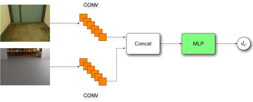
At first glance, it may seem that by moving from single images to image pairs as input, we are solving a more difficult learning problem. But in fact, the Siamese network is not more complex. Its number of parameters is similar to the conventional classification network, it outputs only a scalar value, and by looking at pairs we have quadratically increased the number of training samples. Importantly, sampling pairs of training images reduces spurious correlations. As a simplified cartoon example, consider a case where one can see the sky behind the door in many training examples of the “open” state. A direct classifier will learn that a blue region boosts the score for “open” – which is correct for the training set, but may hurt performance in a previously unseen environment with blue doors. Whereas the pair classifier can at most learn that a blue region being present in only one of the two images boosts the score for “different”, which is likely to be true even in the new environment.
Efficient similarity-based classification. An important question is how to utilise the learned similarity function in an efficient manner to classify an unseen test example . The obvious approach would be some sort of -nearest neighbour scheme. However, that is fairly inefficient, because to find the nearest neighbours one has to compute the similarities from the test sample to all training examples, each corresponding to a forward pass of the network. Alternatively, one can chose one (or a few) representatives for each class and compute the similarities only to them, as often done in few-shot classification. By representing each class with a single representative, one potentially sacrifices robustness to gain speed. Particularly when working with highly non-linear deep embeddings, it is not obvious how to find the best representatives. In fact it is not even clear that any fixed, small set of exemplars works for all test examples.
A main finding of the present work is that it is not necessary to find a privileged set of “nearest” or “suitable” class exemplars for similarity computation. Rather, we observe that good results are achieved by using the average similarity to any random subset of class representatives in the training set. This includes the (inefficient) extreme case of using the average similarity over all class exemplars, as well as the opposite extreme of blindly sampling a single exemplar per class for every new query. It thus appears that the CNN embedding preserves, at least approximately, a global notion of distance; and that it indeed manages to separate the classes by wide margins, such that most individual similarities yield a correct class assignment.
| exemplars | similarity | test example | similarity | exemplars |
|---|---|---|---|---|
| Katakana | (Katakana) | Korean | ||
|
|
|||
|
|
|
||
|
|
|||
Technically, one simply samples representatives at random from the training samples of each class . Similarities are computed for all of them by passing and through the Siamese network. This yields similarity scores per class, which are averaged to obtain a classification score:
| (3) |
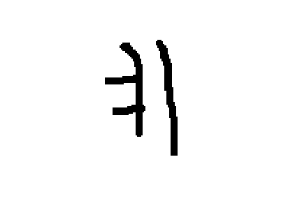
The classification rule then assigns the class with the higher average score, . The procedure is illustrated in Fig. 3.
Obviously, one could think of many other possible consensus mechanisms. E.g., one might interpret the CNN output as probability of being in the same, respectively different classes, threshold each of the individual scores with a threshold of , and then perform majority voting (this is sometimes done in ensemble classifiers, for instance Random Forests). We experimented also with the latter scheme and found that it performs similar to averaging, see Table 1. Actually, the fact that even sampling a single random exemplar per class () works well indicates that the embedding separates the classes with a healthy margin, such that voting will also work. We note that voting may be less robust in some situations. The early rounding from soft to hard, binary similarity scores may be problematic if the scores are not well calibrated to probabilities, such that is not the optimal threshold. Moreover, voting with few exemplars can lead to ties. Further research is required, in particular one might also try to learn the consensus mechanism along with the Siamese embedding. At this point, we prefer averaging, which appears to be the safer option when applied to an unknown dataset.
Architectures. Both our baseline and our Siamese similarity network are based on the VGG16 architecture. The Siamese variant has two tied VGG16 branches. Their outputs are concatenated (subtracting them works equally well) and fed through a multi-layer perceptron with three fully connected layers to obtain the final scores. Training is done with the ADAM variant of stochastic gradient descent, with minibatches of size 16 for the Siamese network, respectively 32 for the single-branch baseline. The smaller batch size is meant to ensure a fair comparison in terms of ressources, since image pairs need twice as much memory. GPU memory is the bottleneck for CNN training when working with large images (like our “doors” dataset). For the “Learning to Compare” baseline we use the architecture and hyper-parameters of the original, publicly available code.
Pre-training. It is standard practice to pre-train deep neural networks with very large databases to improve their performance, even if those databases are not perfectly matched to the actual task. The pre-training is completed by the actual training with a smaller amount of task-specific data.
Also for the Siamese network, existing, large databases can be exploited for pre-training. Empirically, pre-training the individual branches with a conventional classification task (respectively, using pre-trained layers from standard classification architectures) does not improve over random initialisation. On the contrary, it is beneficial to pre-train the similarity network with external data, unless one has a very large training set. For our purposes, we used ImageNet to randomly generate pairs belonging to the same class, respectively different classes. We pre-train the network with these pairs to predict the probability that the two inputs belong to different classes, using the conventional cross-entropy loss. Then, the same pairwise similarity training is repeated with the actual training data of the target problem to fine-tune to the application setting. In our experiments, pre-training improves performance on all datasets, by 10 percent points. For completeness, we note that only ImageNet pre-training, without subsequent tuning on task-specific data, is not enough and barely better than random chance.
4 Experiments
We conducted experiments on four different datasets (greyscale, RGB, and RGB-D) to evaluate the proposed classification scheme. The consistent improvements on a wide variety of datasets and inputs indicates that the method is fairly general and not limited to particular classes or image characteristics. For each dataset we construct a binary task that corresponds to our goal of operating under domain-shift, i.e., the training set shows how to separate the classes, but does not show the full within-class variability. Beyond our actual application of doors, we used public datasets to ensure the results are repeatable and can be compared against. Those public datasets were not designed with domain shift in mind. We did our best to design tasks that are challenging and representative of real applications.
| doors | NYU2 | Pasadena | OmniInst | OmniSymb | |
| Baseline | 86.1 | 76.7 | 85.0 | 84.4 | 72.3 |
| LtC,=10 | 64.3 | 72.9 | 79.7 | 81.5 | 66.9 |
| Siamese, avg,=1 | 90.6 | 82.2 | 90.7 | 94.6 | 79.6 |
| Siamese, avg,=10 | 90.9 | 83.3 | 90.7 | 94.6 | 79.8 |
| Siamese, avg, all | 91.1 | 82.2 | 89.5333Using all (2000) examples not tractable, we set =100. | 94.3 | 79.9 |
| Siamese, vote,=10 | 91.0 | 83.3 | 89.8 | 94.7 | 79.9 |
| Siamese, vote, all | 90.7 | 82.2 | 89.533footnotemark: 3 | 94.7 | 79.8 |
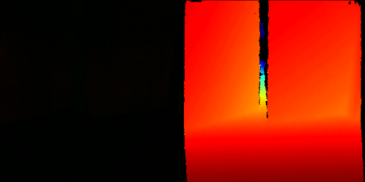
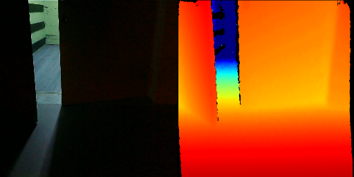
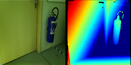
Open and Closed Doors is a new dataset collected for the experiment that sparked this work and served as running example in the paper. The goal is to determine whether a door is closed or open. The dataset consists of RGB-D images acquired by a real mobile robot (Fig. 1), and includes hinged doors and roll-up doors. There are multiple images per door with varying lighting and open/closed status conditions, recorded at two different locations (physically different warehouses) and with an unbalanced class distribution with only 25% open instances (in both locations). We designate one location as training set, and the other one as test set. Since each location only has a limited number of doors (11 doors / 850 images for training, respectively 10 doors / 792 images for testing) which vary in appearance between locations, there is a clear domain shift and we expect conventional classification to overfit to the closed world of the training location.
As can be seen from the results in Table 1, similarity learning significantly increases the classification performance, reducing the mis-classification rate from 13.9% to 9%. In more detail, the baseline and the Siamese similarity network give the same answer for 74.0% of the test set. But in 18.3% of cases the Siamese network is right when the baseline is wrong, whereas the opposite is true only for 7.0% of the data. See Fig. 4 for examples. Visually, one can see that the Siamese network handles bad lighting conditions better, whereas the direct classification apparently relies too strongly on the RGB image and fails if it is under-exposed, which happens sometimes at the test location. Conversely, the Siamese network is seemingly more confused by strong artifacts in the depth channel. Surprisingly, both methods are wrong only on 0.6% of the data, which suggests that they are to a large degree complementary. It is a promising future direction to explore whether this can be exploited by somehow combining them.
Using more random exemplars per class only slightly improves performance. Even at the method performs almost as well as when considering similarities to all training examples, indicating that the CNN embedding separates the two classes rather well.
 |
 |
 |
| Siamese correct | Siamese correct | Siamese wrong |
 |
 |
|
| office | home office |
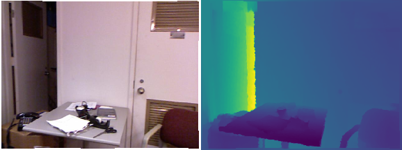
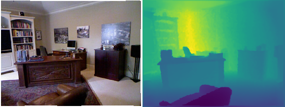
NYU2 is a public dataset [17] that consists of RGB-D images showing different types of indoor scenes (like “kitchen”, “hallway”, etc.). We select the rather challenging task to tell apart the two classes office and home office. Since both are GPS-denied indoor environments, this may for instance be useful for self-localisation. There are 50 instances of home office and 78 instances of office in the dataset. We train on 30% of them (16 home office, 26 office) and then test on the remaining ones. Since the dataset is very small, we randomly split into train and test portions and trust that there will be some degree of domain shift between them, where the training set exhibits unintended biases not replicated in the test data. Due to the small amount of data, we reduce the minibatch size to 8.
Also for this dataset, the Siamese approach reduces the error rate, from 23.3% to 16.5%. Interestingly, a moderate number of exemplars seems to be working slightly better than using fewer, or more. This remains to be investigated further in future work.
 |
 |
|
| Mexican Fan Palm | Camphor Tree |
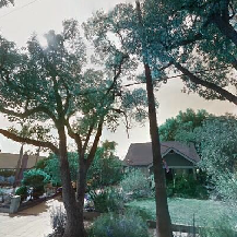
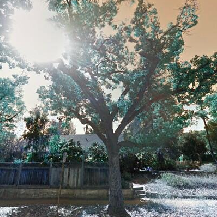
Pasadena Street Trees [18] provides RGB images of different tree species, cropped from Google Streetview panoramas. We define an environment mapping task, to distinguish the two frequent species Camphor Tree (6745 examples) and Mexican Fan Palm (7595 examples). We train on 30% of both classes and then test on the data rest, chosen at random.
This dataset is a good example that even training sets of apparently reasonable size may not be enough to ensure a stable domain, especially when operating in the wild under weakly controlled conditions. Due to the high variability of both the trees and the background, the Siamese similarity learning significantly outperforms a direct class prediction, even though there are 2500 training images per class. The error rate is reduced from 15% to 9.5%. Due to the comparatively big volume of data, it is not tractable to compute the similarities to all training examples, hence we approximated them by setting , which still takes 3 seconds per test image on a Titan Xp GPU. Fortunately, the experiment again confirms that small exemplar sets are sufficient to achieve good results.
 |
 |
|
| Katakana | Korean |
 |
 |
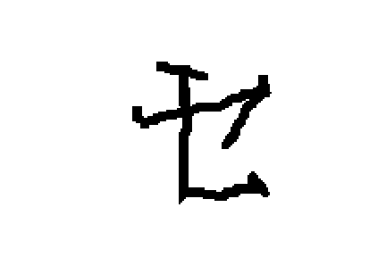
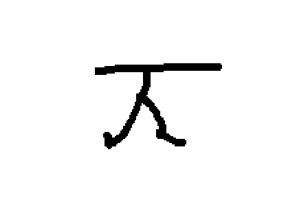
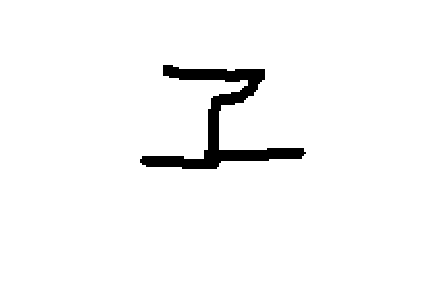
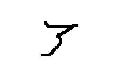
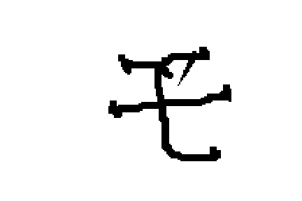
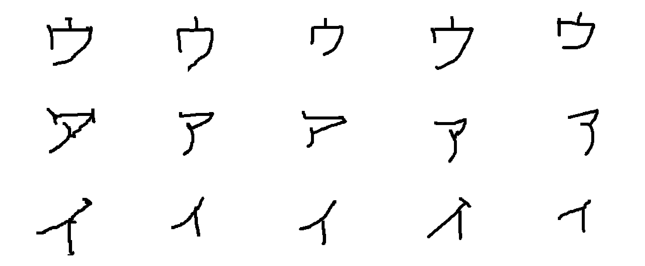
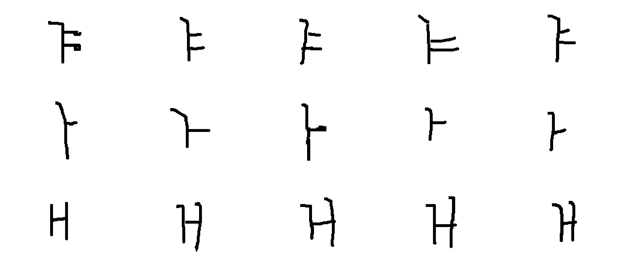
Omniglot [19] is one of the most popular datasets for distance, respectively similarity learning. It consists of greyscale images of handwritten characters from 50 different alphabets. For each character there are 20 different instances (writers). We define two different tasks with domain shift. In both cases the goal is to distinguish Korean characters from Japanese Katakana characters. The alphabets were chosen because they are known to be visually similar and therefore hard to distinguish. The two tasks are defined as follows:
-
•
Inst: randomly select 280 Katakana + 240 Korean instances (30% of total) for training, and the remaining 660 + 560 for testing. I.e., the domain shift arises from the fact that 7 writers are not enough to capture all legitimate variations in writing style. Exemplars are drawn at random, so the chance is low (%) that a test image is paired with a training image of the same character. Still, the network has seen all characters of both languages during training.
-
•
Symb: randomly select 14 Katakana + 12 Korean characters (30% of total) for training and the other 33 + 28 for testing. This creates a more difficult domain shift: the network must learn the “stylistic commonalities” of Japanese, respectively Korean characters from only 30% of the alphabet, such that they generalise to the remaining 70% of which the network has never seen any instance.
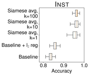
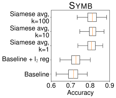
On this dataset the Siamese approach does particularly well. For the Inst scenario it reduces the error rate by two thirds, from 15.6% to 5.5%. For the particularly difficult Symb scenario, the error rate drops from 27% to 18.5%. Recall that the latter is indeed a very challenging problem: the classifier only ever sees 30% of the symbols from the two alphabets, and must learn to assign a symbol it has never seen before to the right alphabet. Under these circumstances, the performance is quite remarkable, compared to chance level.
| Baseline | avg | voting | LtC | |
|---|---|---|---|---|
| k=1 | 84.4 | 94.6 | — | 77.9 |
| k=10 | 84.4 | 94.6 | 94.7 | 81.5 |
| k=100 (all for our method) | 84.4 | 94.3 | 94.7 | 80.7 |
We have argued that heavy regularisation of the direct classification baseline cannot be expected to overcome domain shift. To test this claim, we ran the baseline without regularisation and with -regularisation of the weights. The strength of the regularizer is tuned for best performance by grid search. To exclude biases due to a particular train/test split and to assess how significant the differences are, we perform 100 different random splits, for both the symb and inst task. In Fig. 8 one can see that regularisation only slightly improves the classification at test time, and that the advantage of the Siamese similarity approach is persistent across different splits. This supports our assertion that regularisation is not enough to cope with domain shift.
In few-shot learning terminology, our method is a form of the 2-way, k-shot scenario. As further baseline, we therefore run the “Learning to Compare” (LtC) [14] code. We tested three settings for LtC on OmniglotInst, . We find that LtC cannot beat the direct baseline even when choosing a high , and never reaches the performance of our simple Siamese network. See Tab. 2. Experiments on other datasets confirm this result, see Tab. 1.
The experiment illustrates the difference between the domain shift and few-shot problems. In our setting, we do have a larger training set of class examples, which are all used to learn the best possible similarity function. Only at test time we sample a small set , for efficiency and empirically without loss of accuracy. Whereas LtC learns a similarity mostly from other classes, which is then tuned to only exemplars of the target classes. Therefore, it cannot recover the data manifold as well, and has less knowledge of the intra- and inter-class variations beyond the exemplars. Moreover, LtC consumes more GPU memory, because the complete support set is stored for the forward pass.
5 Conclusion
We have argued that a machine vision system that operates in the wild will in some situations face visual domain shift, since it is not always possible to capture all the variability of the system’s future environment at training time. We have investigated similarity learning with a Siamese CNN as a way of learning classifiers that perform well in the presence of domain shifts. We found that the network embeds the training data in such a way that they are well separated and (relative) similarities are fairly reliable between arbitrary pairs of data points. Hence, an unseen test case can be classified by sampling similarities to few random exemplars from the training data. In experiments on four datasets, deep similarity learning consistently outperforms direct classification.
There are several open points that merit further investigation. First, our study was limited to binary classification. While it is conceptually straight-forward to generalise the idea of similarity learning to multiple classes, it is much less clear how to best implement it. One possibility is to decompose it into multiple pairwise similarities, which will however exponentially increase the number of pairings that must be trained. Another idea would be to directly learn a set of similarities, or a ranking, using exemplars from all classes as additional input. A second point concerns the use of multiple exemplars. Although in our study sampling exemplars brought only minor improvements, it may be a mechanism to robustify the classification in scenarios where the classes are not well separable. In that situation the question arises how to best combine the per-exemplar similarities. Here, we have tested straight-forward, handcrafted averaging and voting schemes. It may however be interesting to also learn the combination, or even to explore an “early combination” where a multi-way similarity [20] is computed from a test example to a set of multiple exemplars.
References
- [1] Gregory Koch, Richard Zemel, and Ruslan Salakhutdinov. Siamese neural networks for one-shot image recognition. In ICML Deep Learning Workshop, 2015.
- [2] Luca Bertinetto, João F. Henriques, Jack Valmadre, Philip H. S. Torr, and Andrea Vedaldi. Learning feed-forward one-shot learners. In NIPS, 2016.
- [3] Oriol Vinyals, Charles Blundell, Timothy Lillkicrap, Koray Kavukcuoglu, and Daan Wierstra. Matching networks for one shot learning. In NIPS, 2016.
- [4] Flood Sung, Yongxin Yang, Li Zhang, Tao Xiang, Philip H. S. Torr, and Timothy M. Hospedales. Learning to compare: relation network for few-shot learning. In CVPR, 2018.
- [5] Liu Yang and Rong Jin. Distance metric learning: A comprehensive survey. Technical report, Michigan State Universiy, 2006.
- [6] Bernhard Schölkopf, Alexander Smola, and Klaus-Robert Müller. Nonlinear component analysis as a kernel eigenvalue problem. Neural Computation, 10(5), 1998.
- [7] Sam T Roweis and Lawrence K Saul. Nonlinear dimensionality reduction by locally linear embedding. Science, 290(5500), 2000.
- [8] Laurens Maaten. Learning a parametric embedding by preserving local structure. In AISTATS, 2009.
- [9] Eric P Xing, Michael I Jordan, Stuart J Russell, and Andrew Y Ng. Distance metric learning with application to clustering with side-information. In NIPS, 2003.
- [10] G Lebanon. Flexible metric nearest neighbor classification. In UAI, 2003.
- [11] Jane Bromley, Isabelle Guyon, Yann LeCun, Eduard Säckinger, and Roopak Shah. Signature verification using a" siamese" time delay neural network. In NIPS, 1994.
- [12] Jure Zbontar and Yann LeCun. Computing the stereo matching cost with a convolutional neural network. In CVPR, 2015.
- [13] Tsung-Yi Lin, Yin Cui, Serge Belongie, and James Hays. Learning deep representations for ground-to-aerial geolocalization. In CVPR, 2015.
- [14] Sergey Zagoruyko and Nikos Komodakis. Learning to compare image patches via convolutional neural networks. In CVPR, 2015.
- [15] Wenjie Luo, Alexander G Schwing, and Raquel Urtasun. Efficient deep learning for stereo matching. In CVPR, 2016.
- [16] Wilfried Hartmann, Silvano Galliani, Michal Havlena, Luc Van Gool, and Konrad Schindler. Learned multi-patch similarity. In ICCV, 2017.
- [17] Pushmeet Kohli Nathan Silberman, Derek Hoiem and Rob Fergus. Indoor segmentation and support inference from rgbd images. In ECCV, 2012.
- [18] Jan D Wegner, Steven Branson, David Hall, Konrad Schindler, and Pietro Perona. Cataloging public objects using aerial and street-level images-urban trees. In CVPR, 2016.
- [19] Brenden M Lake, Ruslan Salakhutdinov, and Joshua B Tenenbaum. Human-level concept learning through probabilistic program induction. Science, 350(6266), 2015.
- [20] Wilfried Hartmann, Silvano Galliani, Michal Havlena, Luc Van Gool, and Konrad Schindler. Learned multi-patch similarity. In ICCV, 2017.