Shape of the quark gluon plasma droplet reflected in the high-$p_{\perp}$ data

Abstract

We show, through analytic arguments, numerical calculations, and comparison with experimental data, that the ratio of the high-$p_{\perp}$ observables $v_{2}/(1-R_{\mathrm{AA}})$ reaches a well-defined saturation value at high $p_{\perp}$, and that this ratio depends only on the spatial anisotropy of the quark gluon plasma (QGP) formed in ultrarelativistic heavy-ion collisions. With expected future reduction of experimental errors, the anisotropy extracted from experimental data will further constrain the calculations of initial particle production in heavy-ion collisions and thus test our understanding of QGP physics.

Introduction: The major goal of relativistic heavy-ion physics QGP1 ; QGP2 ; QGP3 ; QGP4 is understanding the properties of the new form of matter called quark-gluon plasma (QGP) Collins ; Baym , which, in turn, allows understanding properties of QCD matter at its most basic level. Energy loss of rare high-momentum partons traversing this matter is known to be an excellent probe of its properties. Different observables such as the nuclear modification factor $R_{\mathrm{AA}}$ and the elliptic flow parameter $v_{2}$ of high-$p_{\perp}$ particles, probe the medium in different manners, but they all depend not only on the properties of the medium, but also on the density, size, and shape of the QGP droplet created in a heavy-ion collision. Thus drawing firm conclusions of the material properties of QGP is very time consuming and requires simultaneous description of several observables. It would therefore be very useful if there were an observable, or combination of observables, which would be sensitive to only one or just a few of all the parameters describing the system.

For high-$p_{\perp}$ particles, spatial asymmetry leads to different paths, and consequently to different energy losses. Consequently, $v_{2}$ (angular differential suppression) carries information on both the spatial anisotropy and material properties that affect energy loss along a given path. On the other hand, $R_{\mathrm{AA}}$ (angular average suppression) carries information only on material properties affecting the energy loss DREENAc ; DREENAb ; Thorsten ; Molnar , so one might expect to extract information on the system anisotropy by taking a ratio of expressions which depend on $v_{2}$ and $R_{\mathrm{AA}}$. Of course, it is far from trivial whether such intuitive expectations hold, and what combination of $v_{2}$ and $R_{\mathrm{AA}}$ one should take to extract the spatial anisotropy. To address this, we here use both analytical and numerical analysis to show that the ratio of $v_{2}$ and $1-R_{\mathrm{AA}}$ at high $p_{\perp}$ depends only on the spatial anisotropy of the system. This approach provides a complementary method for evaluating the anisotropy of the QGP fireball, and advances the applicability of high-$p_{\perp}$ data to a new level as, up to now, these data were mainly used to study the jet-medium interactions, rather than inferring bulk QGP parameters.

Anisotropy and high-$p_{\perp}$ observables: In DREENAb ; NewObservable , we showed that at very large values of transverse momentum $p_{\perp}$, the fractional energy loss $\Delta E/E$ (which is very complex, both analytically and numerically, due to inclusion of multiple effects, see Numerical results for more details) shows asymptotic scaling behavior

$$\Delta E/E\approx\chi(p_{\perp})\langle T\rangle^{a}\langle L\rangle^{b},$$ (1)

where $\langle L\rangle$ is the average path length traversed by the jet, $\langle T\rangle$ is the average temperature along the path of the jet, $\chi$ is a proportionality factor (which depends on initial jet $p_{\perp}$), and $a$ and $b$ are proportionality factors which determine the temperature and path-length dependence of the energy loss. Based on Refs. BDMPS ; ASW ; GLV ; HT , we might expect values like $a=3$ and $b=1$ or $2$, but a fit to a full-fledged calculation yields values $a\approx 1.2$ and $b\approx 1.4$ NewObservable ; MD_5TeV . Thus the temperature dependence of the energy loss is close to linear, while the length dependence is between linear and quadratic. To evaluate the path length we follow Ref. ALICE_charm :

$$L(x,y,\phi)=\frac{\int_{0}^{\infty}\mathrm{d}\lambda\,\lambda\,\rho(x+\lambda\cos(\phi),y+\lambda\sin(\phi))}{\int_{0}^{\infty}\mathrm{d}\lambda\,\rho(x+\lambda\cos(\phi),y+\lambda\sin(\phi))},$$ (2)

which gives the path length of a jet produced at point $(x,y)$ heading to direction $\phi$, and where $\rho(x,y)$ is the initial density distribution of the QGP droplet. To evaluate the average path length we take average over all directions and production points.

If $\Delta E/E$ is small (i.e., for high $p_{\perp}$ and in peripheral collisions), we obtain DREENAc ; DREENAb ; NewObservable

$$R_{\mathrm{AA}}\approx 1-\xi\langle T\rangle^{a}\langle L\rangle^{b},$$ (3)

where $\xi=(n-2)\chi/2$, and $n$ is the steepness of a power law fit to the transverse momentum distribution, $\mathrm{d}N/\mathrm{d}p_{\perp}\propto 1/p_{\perp}^{n}$. Thus $1-R_{\mathrm{AA}}$ is proportional to the average size and temperature of the medium. To evaluate the anisotropy we define the average path lengths in the in-plane and out-of-plane directions,

$$\langle L_{in}\rangle = \frac{1}{\Delta\phi}\int_{-\Delta\phi/2}^{\Delta\phi/2}\!\!\!\!\mathrm{d}\phi\,\langle L(\phi)\rangle$$ (4)

$$\langle L_{out}\rangle = \frac{1}{\Delta\phi}\int_{\pi/2-\Delta\phi/2}^{\pi/2+\Delta\phi/2}\!\!\!\!\mathrm{d}\phi\,\langle L(\phi)\rangle,$$

where $\Delta\phi=\pi/6$ PHENIX is the acceptance angle with respect to the event plane (in-plane) or orthogonal to it (out-of-plane), and $\langle L(\phi)\rangle$ the average path length in $\phi$ direction. Note that the obtained calculations are robust with respect to the precise value of the small angle $\pm\Delta\phi/2$, but we still keep a small cone $(\pm\pi/12)$ for $R_{\mathrm{AA}}^{in}$ and $R_{\mathrm{AA}}^{out}$ calculations, to have the same numerical setup as in our Ref. DREENAb . Now we can write $\langle L\rangle=(\langle L_{out}\rangle+\langle L_{in}\rangle)/2$ and $\Delta L=(\langle L_{out}\rangle-\langle L_{in}\rangle)/2$. Similarly, the average temperature along the path length can be split to average temperatures along paths in in- and out-of-plane directions, $\langle T_{in}\rangle=\langle T\rangle+\Delta T$ and $\langle T_{out}\rangle=\langle T\rangle-\Delta T$. When applied to an approximate way to calculate $v_{2}$ of high-$p_{\perp}$ particles Christiansen:2013hya , we obtain 

$$v_{2} \approx \frac{1}{2}\frac{R_{\mathrm{AA}}^{in}-R_{\mathrm{AA}}^{out}}{R_{\mathrm{AA}}^{in}+R_{\mathrm{AA}}^{out}}\approx\frac{\xi\langle T_{out}\rangle^{a}\langle L_{out}\rangle^{b}-\xi\langle T_{in}\rangle^{a}\langle L_{in}\rangle^{b}}{4}$$ (5)

$$\approx \xi\langle T\rangle^{a}\langle L\rangle^{b}\left(\frac{b}{2}\frac{\Delta L}{\langle L\rangle}-\frac{a}{2}\frac{\Delta T}{\langle T\rangle}\right),$$

where we have assumed that $\xi\langle T\rangle^{a}\langle L\rangle^{b}\ll 1$, and that $\Delta L/\langle L\rangle$ and $\Delta T/\langle T\rangle$ are small as well.

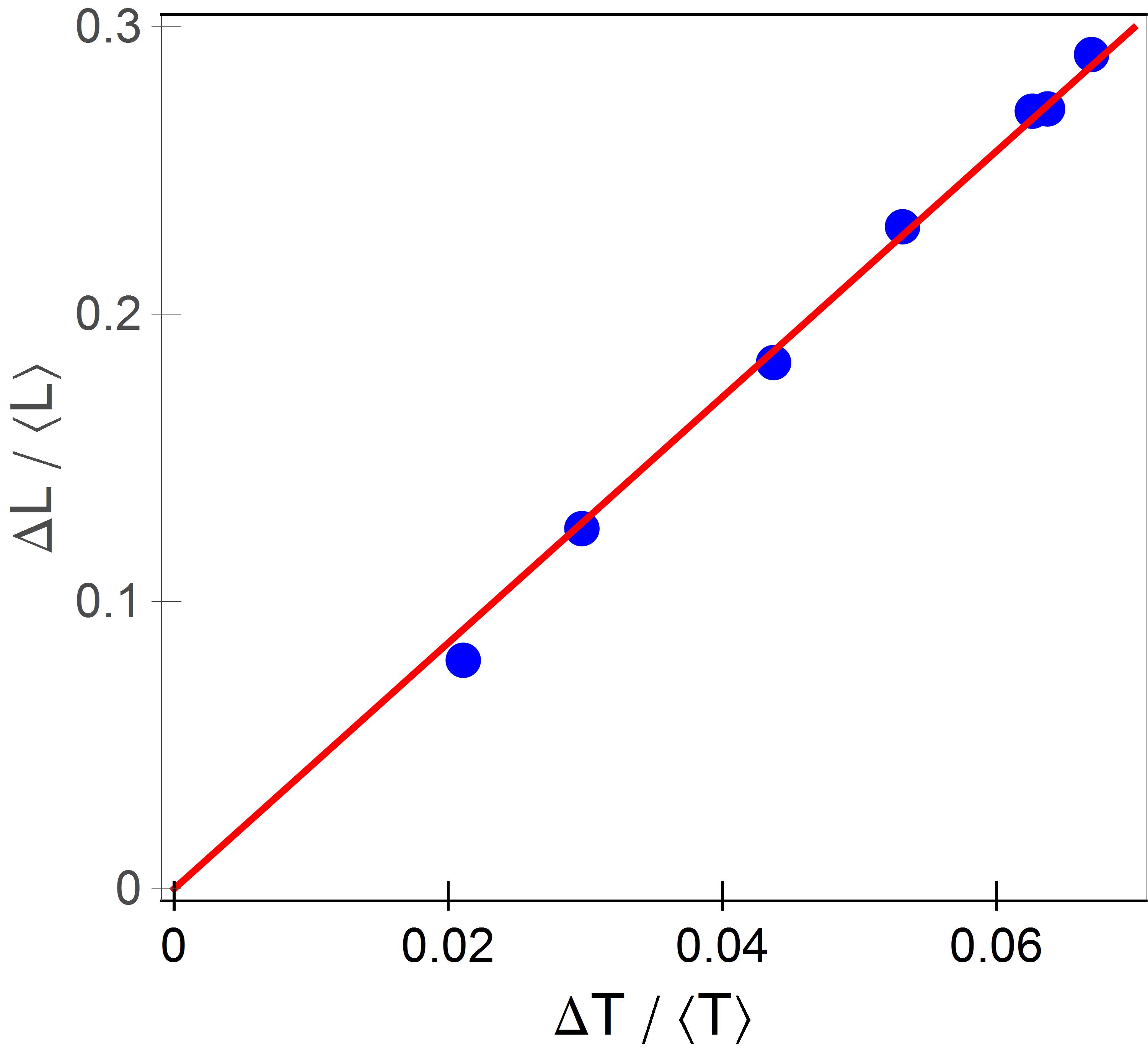
Figure 1: $\Delta T/\langle T\rangle$ vs. $\Delta L/\langle L\rangle$ in Pb+Pb collisions at $\sqrt{s_{\mathrm{NN}}}=5.02$ TeV collision energy at various centralities DREENAc ; DREENAb . The more peripheral the collision, the larger the values. The red solid line depicts linear fit to the values.

By combining Eqs. (3) and (5), we obtain:

$$\frac{v_{2}}{1-R_{\mathrm{AA}}}\approx\left(\frac{b}{2}\frac{\Delta L}{\langle L\rangle}-\frac{a}{2}\frac{\Delta T}{\langle T\rangle}\right).$$ (6)

This ratio carries information on the anisotropy of the system, but through both spatial ($\Delta L/\langle L\rangle$) and temperature ($\Delta T/\langle T\rangle$) variables. From Eq. (6), we see the usefulness of the (approximate) analytical derivations, since the term $(1-R_{\mathrm{AA}})$ in the denominator could hardly have been deduced intuitively, or pinpointed by numerical trial and error. Figure 1 shows a linear dependence $\Delta L/\langle L\rangle\approx c\Delta T/\langle T\rangle$, where $c\approx 4.3$, with the temperature evolution given by one-dimensional Bjorken expansion, as sufficient to describe the early evolution of the system. Eq. (6) can thus be simplified to

$$\frac{v_{2}}{1-R_{\mathrm{AA}}} \approx \frac{1}{2}\left(b-\frac{a}{c}\right)\frac{\langle L_{out}\rangle-\langle L_{in}\rangle}{\langle L_{out}\rangle+\langle L_{in}\rangle}\approx 0.57\varsigma,$$

$${\rm where}\,\;\;\varsigma = \frac{\langle L_{out}\rangle-\langle L_{in}\rangle}{\langle L_{out}\rangle+\langle L_{in}\rangle}\;\;\;{\rm and}\;\;\;\frac{1}{2}(b-\frac{a}{c})\approx 0.57,\;\;\;\;\;\;$$ (7)

when $a\approx 1.2$ and $b\approx 1.4$. Consequently, the asymptotic behavior of observables $R_{\mathrm{AA}}$ and $v_{2}$ is such that, at high $p_{\perp}$, their ratio is dictated solely by the geometry of the fireball. Therefore, the anisotropy parameter $\varsigma$ can be extracted from the high-$p_{\perp}$ experimental data.

Figure 2: Theoretical predictions for $v_{2}/(1-R_{AA})$ ratio of charged hadrons as a function of transverse momentum $p_{\perp}$ compared with $5.02$ TeV $Pb+Pb$ ALICE ALICE_CH_RAA ; ALICE_CH_v2 (red triangles), CMS CMS_CH_RAA ; CMS_CH_v2 (blue squares) and ATLAS ATLAS_CH_RAA ; ATLAS_CH_v2 (green circles) data. Panels correspond to 10-20%, 20-30%, 30-40% and 40-50% centrality bins. The gray band corresponds to the uncertainty in the magnetic to electric mass ratio $\mu_{M}/\mu_{E}$. The upper (lower) boundary of the band corresponds to $\mu_{M}/\mu_{E}=0.4$ ($0.6$) Maezawa ; Nakamura . In each panel, the red line corresponds to the limit $0.57\varsigma$ from Eq. (7).

Regarding the parametrization used to derive Eq. (7) (constants $a$, $b$ and $c$), we note that $a$ and $b$ are well established within our dynamical energy loss formalism and follow from $R_{\mathrm{AA}}$ predictions that are extensively tested on experimental data NewObservable ; MD_5TeV and do not depend on the details of the medium evolution. Regarding $c$, it may (to some extent) depend on the type of the implemented medium evolution, but this will not affect the obtained scaling, only (to some extent) the overall prefactor in Eq. (7).

Numerical results: To assess the applicability of the analytically derived scaling in Eq. (7), we calculate $v_{2}/(1-R_{\mathrm{AA}})$ using our full-fledged numerical procedure for calculating the fractional energy loss. This procedure is based on our state-of-the-art dynamical energy loss formalism MD_Dyn ; MD_Coll , which has several unique features in the description of high-$p_{\perp}$ parton medium interactions: i) The formalism takes into account a finite size, finite temperature QCD medium consisting of dynamical (that is moving) partons, contrary to the widely used static scattering approximation and/or medium models with vacuum-like propagators (e.g. BDMPS ; ASW ; GLV ; HT ). ii) The calculations are based on the finite-temperature generalized hard-thermal-loop approach Kapusta , in which the infrared divergences are naturally regulated MD_Dyn ; MD_Coll ; DG_TM . iii) Both radiative MD_Dyn and collisional MD_Coll energy losses are calculated under the same theoretical framework, applicable to both light and heavy flavor. iv) The formalism is generalized to the case of finite magnetic MD_MagnMass mass, running coupling MD_PLB and towards removing the widely used soft-gluon approximation BDD_sga . The formalism was further embedded into our recently developed DREENA-B framework DREENAb , which integrates initial momentum distribution of leading partons VitevDist , energy loss with path-length ALICE_charm and multi-gluon GLV_suppress fluctuations and fragmentation functions DSS , in order to generate the final medium modified distribution of high-$p_{\perp}$ hadrons. The framework was recently used to obtain joint $R_{AA}$ and $v_{2}$ predictions for $5.02$ TeV Pb+Pb collisions at the LHC DREENAb , showing a good agreement with the experimental data.

We have previously shown Blagojevic_JPG that all the model ingredients noted above have an effect on the high-$p_{\perp}$ data, and thus should be included to accurately explain it. In that respect, our model is different from many other approaches, which use a sophisticated medium evolution, but an (over)simplified energy loss model. Our previous work, however, shows that, for explaining the high-$p_{\perp}$ data, an accurate description of high-$p_{\perp}$ parton-medium interactions is at least as important as an advanced medium evolution model. For example, the dynamical energy loss formalism, embedded in 1D Bjorken expansion, explains well the $v_{2}$ puzzle DREENAb , i.e., the inability of other models to jointly explain $R_{AA}$ and $v_{2}$ measurements. To what extent the dynamical energy loss predictions will change when embedded in full three-dimensional evolution is at the time of this writing still unknown, but our previous results nevertheless make it plausible that calculations employing simple one-dimensional expansion can provide valuable insight into the behavior of jets in the medium.

Our results for longitudinally expanding system (1D Bjorken), and the corresponding data are shown in Fig. 2. The gray band shows our full DREENA-B result (see above) with the band resulting from the uncertainty in the magnetic to electric mass ratio $\mu_{M}/\mu_{E}$ Maezawa ; Nakamura . The red line corresponds to the $0.57\varsigma$ limit from Eq. (7), where $\varsigma$ is the anisotropy of the path lengths used in the DREENA-B calculations DREENAb ; DREENAc . Importantly, for each centrality, the asymptotic regime – where the $v_{2}/(1-R_{\mathrm{AA}})$ ratio does not depend on $p_{\perp}$, but is determined by the geometry of the system – is already reached from $p_{\perp}\sim 20$–30 GeV; the asymptote corresponds to the analytically derived Eq. (7), within $\pm 5\%$ accuracy. It is also worth noticing that our prediction of asymptotic behavior was based on approximations which are not necessarily valid in these calculations, but the asymptotic regime is nevertheless reached, telling that those assumptions were sufficient to capture the dominant features. If, as we suspect, the high-$p_{\perp}$ parton-medium interactions are more important than the medium evolution model in explaining the high-$p_{\perp}$ data, this behavior reflects this importance and the analytical derivations based on a static medium may capture the dominant features seen in Fig. 2.

Furthermore, to check if the experimental data support the derived scaling relation, we compare our results to the ALICE ALICE_CH_RAA ; ALICE_CH_v2 , CMS CMS_CH_RAA ; CMS_CH_v2 and ATLAS ATLAS_CH_RAA ; ATLAS_CH_v2 data for $\sqrt{s_{\mathrm{NN}}}=5.02$ TeV $Pb+Pb$ collisions. The experimental data, for all three experiments, show the same tendency, i.e., the independence on the $p_{\perp}$ and a consistency with our predictions, though the error bars are still large. Therefore, from Fig. 2, we see that at each centrality both the numerically predicted and experimentally observed $v_{2}/(1-R_{\mathrm{AA}})$ approach the same high-$p_{\perp}$ limit. This robust, straight line, asymptotic value carries information about the system’s anisotropy, which is, in principle, simple to infer from the experimental data.

Ideally, the experimental data (here from ALICE, CMS and ATLAS) would overlap with each other, and would moreover have small error bars. In such a case, the data could be used to directly extract the anisotropy parameter $\varsigma$ by fitting a straight line to the high-$p_{\perp}$ part of the $v_{2}/(1-R_{\mathrm{AA}})$ ratio. While such direct anisotropy extraction would be highly desirable, the available experimental data are unfortunately still not near the precision level needed to implement this. However, we expect this to change in the upcoming high-luminosity $3^{\mathrm{rd}}$ run at the LHC, where the error bars are expected to be significantly reduced, so that this procedure can be directly applied to experimental data.

It is worth remembering that the anisotropy parameter $\varsigma$, which can be extracted from the high-$p_{\perp}$ data, is not the commonly used anisotropy parameter $\epsilon_{2}$,

$$\epsilon_{2}=\frac{\langle y^{2}-x^{2}\rangle}{\langle y^{2}+x^{2}\rangle}=\frac{\int\mathrm{d}x\,\mathrm{d}y\,(y^{2}-x^{2})\,\rho(x,y)}{\int\mathrm{d}x\,\mathrm{d}y\,(y^{2}+x^{2})\,\rho(x,y)},$$ (8)

where $\rho(x,y)$ is the initial density distribution of the QGP droplet. We may also expect, that once the transverse expansion is included in the description of the evolution, the path-length anisotropy $\varsigma$ reflects the time-averaged anisotropy of the system, and therefore is not directly related to the initial-state anisotropy $\epsilon_{2}$. Nevertheless, it is instructive to check how the path-length anisotropy in our simple model relates to conventional $\epsilon_{2}$ values in the literature. For this purpose we construct a variable

$$\epsilon_{2L}=\frac{\langle L_{out}\rangle^{2}-\langle L_{in}\rangle^{2}}{\langle L_{out}\rangle^{2}+\langle L_{in}\rangle^{2}}=\frac{2\varsigma}{1+\varsigma^{2}}.$$ (9)

We have checked that for different density distributions $\epsilon_{2}$ and $\epsilon_{2L}$ agree within $\sim$10% accuracy.

We have extracted the parameters $\varsigma$ from the DREENA-B results shown in Fig. 2; the corresponding $\epsilon_{2L}$ results are shown as a function of centrality in Fig. 3 and compared to $\epsilon_{2}$ evaluated using various initial-state models in the literature MCGlauber ; EKRT ; IPGlasma ; MCKLN . Note that conventional (EKRT EKRT , IP-Glasma IPGlasma ) $\epsilon_{2}$ values trivially agree with our initial $\epsilon_{2}$ (not shown in the figure), i.e., the initial $\epsilon_{2}$ characterize the anisotropy of the path lengths used as an input to DREENA-B, which we had chosen to agree with the conventional models . It is, however, much less trivial that, through this procedure, in which we calculate the ratio of $v_{2}$ and $1-R_{AA}$ through full DREENA framework, our extracted $\epsilon_{2L}$ almost exactly recovers our initial $\epsilon_{2}$. Note that $\epsilon_{2}$ is indirectly introduced in $R_{AA}$ and $v_{2}$ calculations through path-length distributions, while our calculations are performed using full-fledged numerical procedure, not just Eq. (1). Consequently, such direct extraction of $\epsilon_{2L}$ and its agreement with our initial (and consequently also conventional) $\epsilon_{2}$ is highly nontrivial and gives us a good deal of confidence that $v_{2}/(1-R_{\mathrm{AA}})$ is related to the anisotropy of the system only, and not its material properties.

Figure 3: Comparison of $\epsilon_{2L}$ (red band) obtained from our method, with $\epsilon_{2}$ calculated using Monte Carlo (MC) Glauber MCGlauber (gray band), EKRT EKRT (the purple band), IP-Glasma IPGlasma (green dot-dashed curve), and MC-KLN MCKLN (blue dotted curve) approaches. MC-Glauber and EKRT results correspond to 5.02 TeV, while IP-Glasma and MC-KLN correspond to 2.76 TeV $Pb+Pb$ collisions at the LHC.

Summary: High-$p_{\perp}$ theory and data are traditionally used to explore interactions of traversing high-$p_{\perp}$ probes with QGP, while bulk properties of QGP are obtained through low-$p_{\perp}$ data and the corresponding models. On the other hand, it is clear that high-$p_{\perp}$ probes are also powerful tomography tools since they are sensitive to global QGP properties. We here demonstrated this in the case of spatial anisotropy of the QCD matter formed in ultrarelativistic heavy-ion collisions. We used our dynamical energy loss formalism to show that a (modified) ratio of two main high-$p_{\perp}$ observables, $R_{\mathrm{AA}}$ and $v_{2}$, approaches an asymptotic limit at experimentally accessible transverse momenta, and that this asymptotic value depends only on the shape of the system, not on its material properties. However, how exactly this asymptotic value reflects the shape and anisotropy of the system requires further study employing full three-dimensional expansion, which is our current work in progress. The experimental accuracy does not yet allow the extraction of the anisotropy from the data using our scheme, but once the accuracy improves in the upcoming LHC runs, we expect that the anisotropy of the QGP formed in heavy-ion collisions can be inferred directly from the data. Such an experimentally obtained anisotropy parameter would provide an important constraint to models describing the early stages of heavy-ion collision and QGP evolution, and demonstrate synergy of high-$p_{\perp}$ theory and data with more common approaches for inferring QGP properties.

Acknowledgments: We thank Jussi Auvinen, Hendrik van Hees, Etele Molnar and Dusan Zigic for useful discussions. We also thank Tetsufumi Hirano and Harri Niemi for sharing their MC-KLN and EKRT results with us. This work is supported by the European Research Council, Grant No. ERC-2016-COG: 725741, and by the Ministry of Science and Technological Development of the Republic of Serbia, under Projects No. ON171004 and No. ON173052.

References

- (1) M. Gyulassy and L. McLerran, Nucl. Phys. A 750, 30 (2005).
- (2) E. V. Shuryak, Nucl. Phys. A 750, 64 (2005).
- (3) B. Jacak and P. Steinberg, Phys. Today 63, 39 (2010).
- (4) C. V. Johnson and P. Steinberg, Physics Today 63, 29 (2010).
- (5) J. C. Collins and M. J. Perry, Phys. Rev. Lett. 34, 1353 (1975).
- (6) G. Baym and S. A. Chin, Phys. Lett. B 62, 241 (1976).
- (7) D. Zigic, I. Salom, J. Auvinen, M. Djordjevic and M. Djordjevic, J. Phys. G 46, 085101 (2019).
- (8) T. Renk, Phys. Rev. C 85, 044903 (2012).
- (9) D. Molnar and D. Sun, Nucl. Phys. A 932, 140 (2014); Nucl. Phys. A 910-911, 486 (2013).
- (10) D. Zigic, I. Salom, J. Auvinen, M. Djordjevic and M. Djordjevic, Phys. Lett. B 791, 236 (2019)
- (11) M. Djordjevic, D. Zigic, M. Djordjevic, J. Auvinen, Phys. Rev. C 99, 061902 (2019).
- (12) R. Baier, Y. Dokshitzer, A. Mueller, S. Peigne, and D. Schiff, Nucl.Phys.B 484, 265 (1997).
- (13) N. Armesto, C. A. Salgado, and U. A. Wiedemann, Physical Review D 69, 114003 (2004).
- (14) M. Gyulassy, P. Lévai, and I. Vitev, Nuclear Physics B 594, 371 (2001).
- (15) X. N. Wang and X. f. Guo, Nucl. Phys. A 696, 788 (2001).
- (16) M. Djordjevic and M. Djordjevic, Phys. Rev. C 92, 024918 (2015).
- (17) A. Dainese [ALICE Collaboration], Eur. Phys. J. C 33, 495 (2004).
- (18) S. Afanasiev et al. [PHENIX Collaboration], Phys. Rev. C 80, 054907 (2009).
- (19) P. Christiansen, K. Tywoniuk and V. Vislavicius, Phys. Rev. C 89, 034912 (2014).
- (20) M. Djordjevic, Phys. Rev. C 80, 064909 (2009); M. Djordjevic and U. Heinz, Phys. Rev. Lett. 101, 022302 (2008).
- (21) M. Djordjevic, Phys. Rev. C 74, 064907 (2006).
- (22) J. I. Kapusta, Finite-Temperature Field Theory (Cambridge University Press, 1989).
- (23) M. Djordjevic and M. Gyulassy, Phys. Rev. C 68, 034914 (2003).
- (24) M. Djordjevic and M. Djordjevic, Phys. Lett. B 709, 229 (2012).
- (25) M. Djordjevic and M. Djordjevic, Phys. Lett. B 734, 286 (2014).
- (26) B. Blagojevic, M. Djordjevic and M. Djordjevic, Phys. Rev. C 99, 024901 (2019).
- (27) Z. B. Kang, I. Vitev and H. Xing, Phys. Lett. B 718, 482 (2012).
- (28) M. Gyulassy, P. Levai and I. Vitev, Phys. Lett. B 538, 282 (2002).
- (29) D. de Florian, R. Sassot and M. Stratmann, Phys. Rev. D 75, 114010 (2007).
- (30) B. Blagojevic and M. Djordjevic, J. Phys. G 42, 075105 (2015).
- (31) Yu. Maezawa et al. [WHOT-QCD Collaboration], Phys. Rev. D 81, 091501 (2010).
- (32) A. Nakamura, T. Saito and S. Sakai, Phys. Rev. D 69, 014506 (2004).
- (33) S. Acharya et al. [ALICE Collaboration], JHEP 1811, 013 (2018).
- (34) S. Acharya et al. [ALICE Collaboration], JHEP 1807, 103 (2018).
- (35) V. Khachatryan et al. [CMS Collaboration], JHEP 1704, 039 (2017).
- (36) A. M. Sirunyan et al. [CMS Collaboration], Phys. Lett. B 776, 195 (2018).
- (37) [ATLAS Collaboration], ATLAS-CONF-2017-012, (unpublished), https://cds.cern.ch/record/2244824.
- (38) M. Aaboud et al. [ATLAS Collaboration], Eur. Phys. J. C 78, 997 (2018).
- (39) C. Loizides, J. Kamin, D. d’Enterria, Phys. Rev. C 97, 054910 (2018).
- (40) K. J. Eskola, H. Niemi, R. Paatelainen and K. Tuominen, Phys. Rev. C 97, 034911 (2018).
- (41) J. E. Bernhard, J. S. Moreland, S. A. Bass, J. Liu and U. Heinz, Phys. Rev. C 94, 024907 (2016)
- (42) T. Hirano, P. Huovinen, K. Murase and Y. Nara, Prog. Part. Nucl. Phys. 70, 108 (2013).