Risk-averse risk-constrained optimal control

Abstract

Multistage risk-averse optimal control problems with nested conditional risk mappings are gaining popularity in various application domains. Risk-averse formulations interpolate between the classical expectation-based stochastic and minimax optimal control. This way, risk-averse problems aim at hedging against extreme low-probability events without being overly conservative. At the same time, risk-based constraints may be employed either as surrogates for chance (probabilistic) constraints or as a robustification of expectation-based constraints. Such multistage problems, however, have been identified as particularly hard to solve. We propose a decomposition method for such nested problems that allows us to solve them via efficient numerical optimization methods. Alongside, we propose a new form of risk constraints which accounts for the propagation of uncertainty in time.

I Introduction

I-A Background, motivation and contributions

Risk measures in stochastic optimal control serve two purposes: firstly, they allow to account for inexact knowledge of the underlying probability distribution — which in most cases is merely estimated — and, secondly, offer a flexible framework which interpolates between worst-case and expectation-based (risk-neutral) formulations [1, 2]. Risk-averse optimal control aims at optimizing the expectation of a (random) cost function accounting for the worst-case probability distribution — a general approach which has been termed distributionally robust optimization [3].

In several applications it is desirable to impose constraints on random quantities in a probabilistic fashion (typically in the form of probabilistic or expectation constraints), yet in doing so one should take into account the ambiguity associated with the probability distribution [4]. Risk constraints can be interpreted as ambiguous expectation constraints [5, 6] and are often employed as surrogates for chance constraints [7, 8] in order to avoid having to resort to computationally demanding methods such as integer programming [9].

Risk-averse optimal control formulations are nowadays making their way in applications such as power systems [10], and economics [2] as their favorable properties are becoming evident. Yet, their applicability is hindered by their complexity and computational cost of associated multistage formulations. Multistage risk-averse optimal control problems amount to the optimization of a composition of several nonsmooth mappings [1]. Typical numerical solution approaches, such as stochastic dual dynamic programming, fall short when faced with large dimension of scenario-based problems [11, 12, 13]. When the involved risk measures are of the average value-at-risk type, we may obtain explicit solutions by multiparametric piecewise quadratic programming; this is, however, limited to systems with with few states and small prediction horizons [14].

The contributions of this paper are twofold: (i) we present a novel framework for risk constraints using nested risk measures which aim at accounting for the propagation of ambiguity; we call this new type of risk constraints, multistage nested risk constraints, (ii) we propose a reformulation of multistage risk-averse problems involving nested risk measures which facilitates their numerical solution.

While much of the research attention has focused on particular risk measures, such as the average value-at-risk [15, 8] and the mean upper semi-deviation [16], it has been unclear how to extend existing results to more general risk measures. Overall, our approach makes use of the dual conic representation of risk measures and allows for the use of arbitrary coherent risk measures in contrast to existing approaches which focus on specific risk measures.

I-B Notation

Let $\N_{[k_{1},k_{2}]}$ denote the integers in $[k_{1},k_{2}]$. For $z\in\Re^{n}$ let $\plus{z}=\max\{0,z\}$, where the max is taken element-wise. We denote the transpose of a matrix $A$ by $A^{{\scriptscriptstyle\top}}$. The dual cone $\mathcal{K}^{*}$ of a closed convex cone $\mathcal{K}\subseteq\Re^{n}$ is the set $\mathcal{K}^{*}=\{y\in\Re^{n}\mid y^{\top}x\geq 0,\forall x\in\mathcal{K}\}$. The relative interior of $\mathcal{K}$ is denoted by $\operatorname{ri}(\mathcal{K})$. A function $f:\Re^{n}\to\Re$ is called lower semicontinuous (lsc) if its lower level sets, $\{x{}\mid{}f(x)\leq\alpha\}$, are closed and it is called level bounded if its lower level sets are bounded.

II Measuring risk

Let $\Omega=\{\omega_{i}\}_{i=1}^{n}$ be a finite sample space equipped with the discrete $\sigma$-algebra $2^{\Omega}$ and a probability measure $\prob$ with $\prob(\{\omega_{i}\})=\pi_{i}$. Without loss of generality, let us assume that $\pi_{i}>0$. The pair $(\Omega,\prob)$ is called a probability space. A vector $p\in\Re^{n}$ is called a probability vector if $p_{i}\geq 0$ for all $i\in\N_{[1,n]}$ and $\sum_{i=1}^{n}p_{i}=1$. The set of all probability vectors in $\Re^{n}$ is called the probability simplex and is denoted by $\mathcal{D}_{n}$. A real-valued random variable over $(\Omega,\prob)$ is a mapping $Z:\Omega\to\Re$ with $Z(\omega_{i})=Z_{i}$; this can be identified by the vector $Z=(Z_{1},\ldots,Z_{n})\in\Re^{n}$.

Suppose that $Z$ corresponds to a random cost. One possible way to extract a characteristic index out of $Z$ which quantifies its magnitude is to compute its expectation, which is

$$\E^{\pi}[{}Z{}]{}={}\pi^{{\scriptscriptstyle\top}}Z.$$

However, the expectation carries no deviation information and may fail to take into account extreme outcomes of the cost which might happen with low probability. At the opposite end, the maximum of $Z$ is defined as

$$\max[{}Z{}]{}={}\max_{i{}={}1,{}\ldots{},n}Z_{i}.$$

However, the maximum disregards the probability distribution and is likely to produce very conservative values.

Risk measures are mappings $\rho:\Re^{n}\to\Re$ which are used to derive a sure outcome which is no worse than $Z$ itself. In other words, a risk measure extracts a characteristic index taking into account the significance of high costs, which may happen with low probability. Trivially, the expectation and the maximum are risk measures.

A risk measure $\rho:\Re^{n}\to\Re$ is said to be convex if for all $Z,Z^{\prime}\in\Re^{n}$, $c\in\Re$, $\lambda\in[0,1]$ the following properties hold

1. Convexity. $\rho[\lambda Z+(1-\lambda)Z^{\prime}]\leq\lambda\rho[Z]+(1-\lambda)\rho[Z^{\prime}]$,

2. Monotonicity. $\rho[Z]\leq\rho[Z^{\prime}]$, whenever $Z_{i}\leq Z^{\prime}_{i}$ for all $i\in\N_{[1,n]}$,

3. Translation equivariance. $\rho[Z+c1_{n}]=\rho[Z]+c$.

A convex risk measure is called coherent if it satisfies the additional axiom [1, Def. 6.4]

1. Positive homogeneity. $\rho[\alpha Z]=\alpha\rho[Z]$ for all $\alpha\geq 0$.

Coherent risk measures are considered well behaving and the coherency axioms are heavily exploited in risk-averse optimization formulations. Certain risk measures may satisfy a stronger monotonicity assumption [17, 18, 1]

1. Strict/strong monotonicity. The risk measure $\rho$ is called strictly (strongly) monotone if $\rho[Z]<\rho[Z^{\prime}]$ whenever $Z\leq Z^{\prime}$, $\prob[Z<Z^{\prime}]>0$ (and $\max Z<\max Z^{\prime}$).

A monotone risk measure $\rho$ can be regularized to produce a strictly monotone risk measure by defining

$$\rho^{\lambda}[Z]=(1-\lambda)\rho[Z]+\lambda\E^{\pi}[Z],$$

for $\lambda\in(0,1]$. Additionally, $\rho^{\lambda}$ preserves the coherency of $\rho$.

An important duality result is that all coherent risk measures can be written as [1, Thm. 6.5]

$$\rho[Z]{}={}\max_{\mu\in\Af(\pi)}\E^{\mu}[Z],$$ (1)

where $\Af(\pi){}\subseteq{}\mathcal{D}_{n}$ is a closed and convex set of probability vectors which contains $\pi$. We call $\Af(\pi)$ the ambiguity set of $\rho$. Equation (1) offers an interpretation of coherent risk measures: a coherent risk measure is the worst-case expectation under inexact knowledge of the underlying probability vector $\mu$. For example, $\max[Z]=\max_{\mu\in\mathcal{D}_{n}}\E^{\mu}[Z]$, that is, the maximum operator reflects the total lack of probabilistic information.

A popular risk measure is the average value-at-risk with parameter $\alpha\in[0,1]$, which is defined as

$$\AVAR_{\alpha}[Z]{}={}\begin{cases}\min\limits_{t\in\Re}t+\nicefrac{{1}}{{\alpha}}\E^{\pi}\plus{Z-t},&\alpha\neq 0\\ \max[Z],&\alpha=0\end{cases}$$ (2)

The ambiguity set of $\AVARa$ is

$$\Af^{\mathrm{avar}}_{\alpha}(\pi){}={}\left\{\mu\in\Re^{n}\left|\textstyle\sum_{i=1}^{n}\mu_{i}=1,0\leq\mu_{i}\leq\frac{\pi_{i}}{\alpha}\right.\right\}.$$ (3)

The average value-at-risk is a coherent, non-strongly monotone (except for $\alpha=1$), risk measure. For $\alpha=1$, $\Af^{\mathrm{avar}}_{1}(\pi)=\{\pi\}$ and $\AVAR_{1}[Z](\pi)=\E[Z]$. The maximal ambiguity set is attained for $\alpha=0$, i.e., $\Af^{\mathrm{avar}}_{0}{}={}\mathcal{D}_{n}$. Therefore, $\AVARa$ interpolates between the risk-neutral expectation operator ($\AVAR_{1}$) and the worst-case maximum ($\AVAR_{0}$).

Figure 1: Set $\Af^{\mathrm{avar}}_{\alpha}(\pi)$ for different values of $\alpha$ on a space $\Omega=\{\omega_{1},\omega_{2},\omega_{3}\}$ with $\pi_{1}=0.2$, $\pi_{2}=0.3$ and $\pi_{3}=0.5$. (The authors are thankful to Christian Hans, who helped with the Tikz code for this figure.)

Risk measures with polytopic ambiguity sets can be fully described by the set of vertices of their ambiguity sets, that is $\Af=\operatorname{conv}\{\mu^{(l)}\}_{l=1}^{\kappa}$ and $\rho[Z]{}={}\max_{l\in\N_{[1,\kappa]}}\E^{\mu^{(l)}}[Z]$. However, the computation of these extreme points is a computationally demanding operation.

Another popular coherent and strongly monotone risk measure is the entropic value-at-risk at level $\alpha\in(0,1]$, denoted by $\EVARa$ [19], whose ambiguity set is given by

$$\Af^{\mathrm{evar}}_{\alpha}(\pi){}={}\left\{\mu\in\mathcal{D}_{n}{}\mid{}\operatorname{D}_{\mathrm{KL}}(\mu{}\|{}\pi){}\leq{}-\ln\alpha\right\},$$ (4)

where

$$\operatorname{D}_{\mathrm{KL}}(\mu\|\pi){}\dfn{}\sum_{i=1}^{n}\mu_{i}\ln\frac{\mu_{i}}{\pi_{i}},$$

is the Kullback-Leibler divergence from $\pi$ to $\mu$. We have $\EVAR_{1}[Z]=\E[Z]$ and $\lim_{\alpha\downarrow 0}\EVARa[Z]=\max[Z]$. The entropic value-at-risk $\EVARa$ is strongly monotone and, additionally, strictly monotone over the space of random variables with $\prob[\{\omega{}\mid{}Z(\omega)=\max[Z]\}]<1-\alpha$ [17].

III Stochastic systems and multistage risk

III-A System dynamics and scenario trees

Consider the following discrete-time dynamical system

$$x_{t+1}{}={}f(x_{t},u_{t},w_{t}),$$ (5)

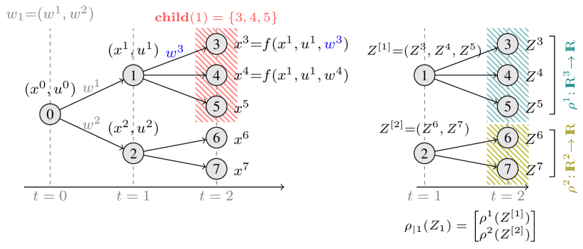
with state variable $x_{t}\in\Re^{n_{x}}$, input $u_{t}\in\Re^{n_{u}}$ and a disturbance $w_{t}\in\Re^{n_{w}}$ which is a random process. We will study the evolution of this system throughout a finite horizon of $N$ future time instants referred to as stages. Starting from a known initial state $x_{0}$ the system states evolve according to (5) as illustrated in Figure 2(a) giving rise to a structure known as a scenario tree. There have been proposed several methodologies to generate scenario trees from data [20, 21].

The nodes of the tree are assigned a unique index $i$ with $i=0$ being the root node which corresponds to the initial state $x_{0}$. The nodes at stage $t\in\N_{[0,N]}$ are denoted by $\operatorname{nodes}(t)$. Starting from the root node, a node $i$ is visited with probability $\pi^{i}>0$ (and $\pi^{0}=1$); this makes $\operatorname{nodes}(t)$ a probability space with probability vector $\pi_{t}=(\pi^{i})_{i\in\operatorname{nodes}(t)}$.

The unique ancestor of a node $i\in\operatorname{nodes}(t)\setminus\{0\}$ is denoted by $\operatorname{anc}(i)$ and the set of children of $i\in\operatorname{nodes}(t)$ for $t\in\N_{[0,N-1]}$ is $\operatorname{child}(i)\subseteq\operatorname{nodes}(t+1)$; this becomes a probability space with probability vector $\pi^{[i]}=\frac{1}{\pi^{i}}(\pi^{i_{+}})_{i_{+}\in\operatorname{child}(i)}$.

As shown in Fig. 2(a), every node $i$ of the tree is associated with a state value $x^{i}$ and all non-leaf nodes $i$ are assigned an input $u^{i}$. Every edge connecting $i$ with $i_{+}{}\in{}\operatorname{child}(i)$ is associated with a disturbance $w^{i_{+}}$. The finite-horizon evolution of (5) on the scenario tree is described by

$$x^{i_{+}}{}={}f(x^{i},u^{i},w^{i_{+}})$$ (6)

for all $i\in\operatorname{nodes}(t)$, $t\in\N_{[0,N-1]}$ and $i_{+}\in\operatorname{child}(i)$. Note that having assigned a control action $u^{i}$ means that decisions are made in a causal fashion, i.e., control actions $u_{t}$ are only allowed to depend on information that is available up to time $t$. The nodes of the tree at stage $N$ are called leaf nodes.

III-B Measuring risk on scenario trees

In this section we introduce the notion of conditional risk mappings which is essential in measuring the risk of a random cost which evolves in time across the nodes of a scenario tree [1, Sec. 6.8.1].

Figure 2: (a) Structure of a scenario tree showing the evolution of the state of the uncertain system (5); (b) definition of a conditional risk mapping at stage $t=1$ on a scenario tree. Note that, for example, $Z^{4}=\ell_{1}(x^{1},u^{1},w^{4})$ and $Z_{1}=(Z^{3},Z^{4},\ldots,Z^{7})$. The conditional risk $\rho_{\mid{}1}$ is a mapping $\rho_{\mid{}1}:\Re^{|\operatorname{nodes}(2)|}\to\Re^{\operatorname{nodes}(1)}$, that is $\rho_{\mid{}1}:\Re^{5}\to\Re^{2}$.

For $t\in\N_{[0,N-1]}$, let $\ell_{t}:\Re^{n_{x}}\times\Re^{n_{u}}\times\Re^{n_{w}}\to\Re$ be a stage cost function and $\ell_{N}:\Re^{n_{x}}\to\Re$ be the terminal cost function. Such cost functions will be used in the following section to construct optimal control problems.

Every node $i\in\operatorname{nodes}(t+1)$, $t\in\N_{[0,N-1]}$ is associated with a cost value $Z^{i}{}={}\ell_{t}(x^{\operatorname{anc}(i)},u^{\operatorname{anc}(i)},w^{i})$. For each $t\in\N_{[0,N-1]}$ we define a random variable $Z_{t}=(Z^{i})_{i\in\operatorname{nodes}(t+1)}$ on the probability space $\operatorname{nodes}(t+1)$. For example, the cost at $t=0$ is the random variable $Z_{0}=(Z^{i})_{i\in\operatorname{nodes}(1)}=(\ell_{0}(x^{0},u^{0},w^{i}))_{i\in\operatorname{nodes}(1)}$. At stage $N$ the terminal cost is the random variable $Z_{N}=(\ell_{N}(x^{i}))_{i\in\operatorname{nodes}(N)}$.

By defining $Z^{[i]}{}\dfn{}(Z^{i_{+}})_{i_{+}\in\operatorname{child}(i)}$, $i\in\operatorname{nodes}(t)$, we partition the variable $Z_{t}=(Z^{[i]})_{i\in\operatorname{nodes}(t)}$ into groups of nodes which share a common ancestor as shown in Fig. 2(b).

Let $\rho^{i}:\Re^{|\operatorname{child}(i)|}{\to}\Re$ be risk measures on the probability space $\operatorname{child}(i)$. For every stage $t\in\N_{[0,N-1]}$ we may define a conditional risk mapping at stage $t$, $\rho_{\mid{}t}:\Re^{|\operatorname{nodes}(t+1)|}\to\Re^{|\operatorname{nodes}(t)|}$, as follows

$$\rho_{\mid{}t}[{}Z_{t}{}]{}={}(\rho^{i}[{}Z^{[i]}{}])_{i\in\operatorname{nodes}(t)}.$$ (7)

This construction is illustrated in Fig. 2(b).

Conditional risk mappings admit a dual representation akin to that in Eq. (1). Provided that all $\rho^{i}$ are coherent risk measures, (7) yields

$$\rho_{\mid{}t}[Z_{t}]{}={}\Big{(}\max_{\mu^{i}\in\Af^{i}(\pi^{[i]})}\E^{\mu^{i}}[Z^{[i]}]\Big{)}_{i\in\operatorname{nodes}(t)},$$ (8)

where $\Af^{i}$ is the ambiguity set of $\rho^{i}$. Conditional risk mappings are used to measure the risk of a multistage stochastic process $\left(Z_{0},\ldots,Z_{t}\right)$ of random costs, which evolves on a scenario tree. Given a sequence $(\rho_{\mid{}0},\ldots,\rho_{\mid{}t})$ of conditional risk mappings, we define

$$\varrho_{t}(Z_{0},\dots,Z_{t}){}={}\rho_{\mid{}0}\big{[}Z_{0}{}+{}\rho_{\mid{}1}[{}\cdots{}{}+{}\rho_{\mid{}t}[{}Z_{t}{}]{}]\big{]}$$

which is called a nested multistage risk measure. We define the composite risk measure at stage $t$ as

$$\bar{\rho}_{t}[{}Z_{t}{}]=\varrho_{k}(0,\dots,0,Z_{t}).$$ (9)

If all $\rho^{i}$ are coherent risk measures, then $\bar{\rho}_{t}$ is a coherent risk measure on $\operatorname{nodes}(t)$ [1].

IV Risk-constrained risk-averse optimal control

IV-A Risk-averse optimal control problems

A risk-constrained risk-averse optimal control problem with horizon $N$ is defined via the following multistage nested formulation [1, Sec. 6.8.1]

$$V^{\star}{}={} \inf_{u_{0}}\rho_{\mid{}0}\bigg{[}\ell_{0}(x_{0},u_{0},w_{0})+\inf_{u_{1}}\rho_{\mid{}1}\Big{[}\ell_{1}(x_{1},u_{1},w_{1})$$

$${}+{} \ldots+\inf_{u_{N-1}}\rho_{\mid{}N-1}\big{[}\ell_{N-1}(x_{N-1},u_{N-1},w_{N-1})$$

$${}+{} \ell_{N}(x_{N})\big{]}\cdots\Big{]}\bigg{]}$$ (10a)

subject to

$$x_{t+1}{}={} f(x_{t},u_{t},w_{t}),$$ (10b)

$$r_{t}[\phi_{j,t}(x_{t},u_{t},w_{t})]{}\leq{} 0,j\in\N_{[1,q_{t}]},$$ (10c)

$$r_{N}[\phi_{j,N}(x_{N})]{}\leq{} 0,j\in\N_{[1,q_{N}]}$$ (10d)

for all $t\in\N_{[0,N-1]}$. Constraints (10c) are risk constraints involving risk measures $r_{t}$ on the probability spaces $\operatorname{nodes}(t+1)$ and $r_{N}$ is a risk measure on $\operatorname{nodes}(N)$. Their role is discussed in Section IV-B. The infima in (10) are taken with respect to causal control functions $u_{t}$.

The above nested formulation amounts to minimizing the nested multistage cost $\varrho_{N-1}(\ell_{0}(x_{0},u_{0},w_{0}),\ldots,\ell_{N}(x_{N}))$ subject to the system dynamics and additional constraints [1, Sec. 6.8]. Replacing the conditional risk mappings, $\rho_{\mid{}t}$, with conditional expectations, $\E_{\mid{}t}$, results in a standard expectation-based problem [22]. Similarly, when the underlying risks are the maximum operators, we obtain a minimax problem [22]. Therefore, risk-averse problems generalize risk-neutral and minimax formulations and contain them as special cases. Moreover, the above formulation enables the stability analysis of associated model predictive control formulations [23, 24].

IV-B Risk constraints

At each stage $t\in\N_{[0,N-1]}$, let us define $q_{t}$ functions $\phi_{j,t}:\Re^{n_{x}}\times\Re^{n_{u}}\times\Re^{n_{w}}\to\Re$, $j\in\N_{[1,q_{t}]}$. At stage $N$, we also define $q_{N}$ functions $\phi_{j,N}:\Re^{n_{x}}\to\Re$, $j\in\N_{[1,q_{N}]}$. Reciting [25], our objective is to impose that “$\phi_{j,t}$ are adequately $\leq{}0$,” for $t\in\N_{[0,N]}$, in a probabilistic sense.

Let $G_{j,t}=\phi_{j,t}(x_{t},u_{t},w_{t})$ be a real-valued random quantity defined at stage $t\in\N_{[0,N-1]}$ and $G_{j,N}=\phi_{j,N}(x_{N})$. Similar to the definition of $Z^{i}$ in Sec. III-B, at every stage $t\in\N_{[0,N-1]}$ and node $i\in\operatorname{nodes}(t+1)$, we assign values $G_{j,t}=((G_{j}^{i})_{i\in\operatorname{nodes}(t+1)}$ for every $j\in\N_{[1,q_{t}]}$. Analogously, we define $G_{j,N}$ for $j\in\N_{[1,q_{N}]}$

Risk constraints may serve several purposes: (i) the average (and the entropic) value-at-risk can be used as a convex approximation of chance constraints [15]. Chance constraints of the form $\prob[G_{j,t}{}\leq{}0]\geq 1-\delta$ can be approximated by risk constraints of the form $\AVAR_{\delta}[G_{j,t}]\leq 0$ (or $\EVAR_{\delta}[G_{j,t}]\leq 0$) — in particular, $\AVAR$ offers a tight convex approximation to chance constraints [26, Sec. 4.3.3], (ii) to impose ambiguous expectation constraints, that is, constraints of the form $\E^{\mu}[G_{j,t}]\leq 0$ for all $\mu$ in a set $\mathcal{M}$ [5], and lastly, (iii) to accommodate ambiguity in chance constraints, i.e., $\prob[G_{j,t}{}\leq{}0]\geq 1-\delta$ for all $\prob\in\mathcal{M}$ [1]. Here, we study two different risk constraint formulations on scenario trees, namely, (i) stage-wise risk constraints, (ii) multistage nested risk constraints.

IV-B1 Stage-wise risk constraints

Stage-wise constraints are imposed at every stage $t\in\N_{[0,N-1]}$ as follows

$$r_{t}[{}G_{j,t}{}]{}\leq{}0,$$ (11)

for $j\in\N_{[1,q_{t}]}$, where $r_{t}:\Re^{|\operatorname{nodes}(t+1)|}\to\Re$ are risk measures and $G_{j,t}\in\Re^{|\operatorname{nodes}(t+1)|}$. At $t=N$, similarly, we impose $r_{N-1}[G_{j,N}]\leq 0$ for $j\in\N_{[1,q_{N}]}$. But, such risk-based constraints do not account for how the probability distribution at stage $t$ is generated in time; indeed, the dependence on previous stages in (11) is disregarded. This can lead to certain pathological cases as we demonstrate in the following section.

IV-B2 Multistage nested risk constraints

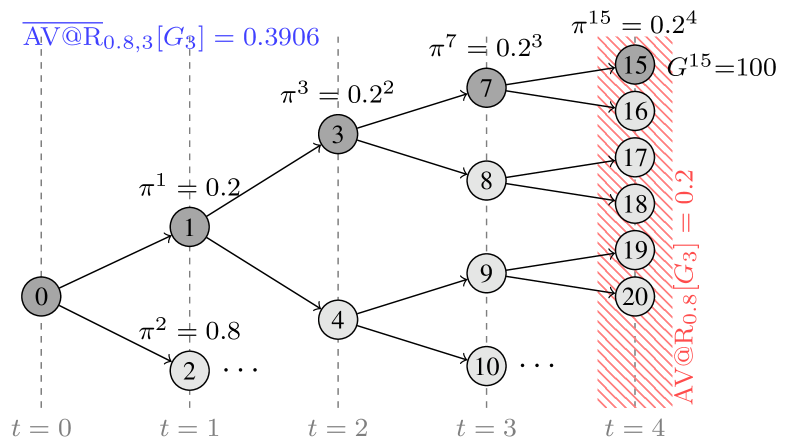
Figure 3: Motivation for the use of multistage nested risk constraints. As explained in Section IV-B2, $G_{3}=(G^{15},G^{16},\ldots)=(100,0,\ldots,0)$.

Consider a scenario tree generated by an iid process $(w_{t})_{t\in\N_{[0,N-1]}}$ with $w_{t}\in\{0,1\}$ as the one in Fig. 3 with $\prob[w_{t}=0]=0.2$ and $\prob[w_{t}=1]=0.8$. Let functions $(\phi_{t})_{t\in\N_{[0,N]}}$ be such that $G^{i}=0$ for $i\neq 15$ and $G^{15}=10^{2}$. The (nominal) probability of node $i=15$ is $\pi^{15}=0.2^{4}=0.0016$. Suppose that the probability has been misestimated and the actual one is $\prob^{\prime}[w_{t}=0]=0.25$ and $\prob^{\prime}[w_{t}=1]=0.75$. This probability vector is within $\Af^{\mathrm{avar}}_{0.8}(\prob)$. On the other hand, we have that $\pi^{\prime{}15}=0.25^{4}=0.0039$, but the ambiguity set $\Af^{\mathrm{avar}}_{0.8}$ on $\operatorname{nodes}(4)$ contains no $\mu$ such that $\mu[\{15\}]=0.0039$. In other words, the stage-wise risk fails to describe how ambiguity may build up and propagate in time. This motivates the introduction of multistage nested risk constraints of the form

$$\bar{r}_{t}[{}G_{j,t}{}]{}={}r_{\mid{}0}\big{[}r_{\mid{}1}\big{[}\cdots{}r_{\mid{}t}[{}G_{j,t}{}]\big{]}\big{]}{}\leq{}0$$ (12)

Here, using the average value-at-risk with parameter $\alpha=0.8$, we compute the risk $\AVAR_{0.8}[G_{3}]\,{=}\,0.2$; the corresponding nested risk is $\overline{\AVAR}_{0.8,3}[G_{3}]\,{=}\,0.3906$. Note that nested risk constraints neither imply nor are implied by stage-wise ones.

V Tractable reformulations

V-A Conic representation of risk measures

The ambiguity set of a coherent risk measure can be written using conic inequalities, i.e., there exist matrices $E,F$ and a vector $b$, such that

$$\rho[Z]{}={}\max_{\mu\in\Re^{n},\nu\in\Re^{r}}\{\mu^{{\scriptscriptstyle\top}}Z{}\mid{}E\mu+F\nu\preccurlyeq_{\mathcal{K}}b\},$$ (13)

where $\mathcal{K}$ is a closed, convex cone and $\nu$ is an auxiliary variable. All widely used coherent risk measures can be written in this form. Tacitly, we have assumed that all admissible $\mu$ in (13) are probability vectors and the ambiguity set of $\rho$ is the following subset of $\mathcal{D}_{n}$

$$\mathcal{A}{}={}\{\mu\in\Re^{n}{}\mid{}\exists\nu\in\Re^{r}{}:{}E\mu+F\nu\preccurlyeq_{\mathcal{K}}b\}.$$

For example, $\AVARa$ is written as in (13) with $r=0$ and $E=\smallmat{I&-I1_{n}}^{{\scriptscriptstyle\top}}$, $b=\smallmat{\nicefrac{{1}}{{\alpha}}\pi^{{\scriptscriptstyle\top}}&01}^{{\scriptscriptstyle\top}}$ and $\mathcal{K}=\Re_{\geq 0}^{2n}\times\{0\}$. $\EVARa$ can also be written in the above form. Let $\mathcal{K}^{\mathrm{e}}=\operatorname{cl}\{(x,y,z)\in\Re^{3}{}\mid{}ye^{x/y}\leq z,y>0\}$ be the exponential cone. By virtue of the equivalence $x\ln(x/y)\leq t\Leftrightarrow(-t,x,y)\in\mathcal{K}^{\mathrm{e}}$, the ambiguity set $\Af^{\mathrm{evar}}_{\alpha}(\pi)$ is

$$\Af^{\mathrm{evar}}_{\alpha}(\pi){}={}\left\{\mu\in\mathcal{D}_{n}\left|{\begin{array}[]{l}\exists\nu\in\Re^{n}:\sum_{i=1}^{n}\nu_{i}{}\leq{}-\ln\alpha,\\ (-\nu_{i},\mu_{i},\pi_{i}){}\in{}\mathcal{K}^{\mathrm{exp}},i\in\N_{[1,n]}\end{array}}\right.\right\}{\!,}$$

Lastly, note that if $\rho$ is admits a conic representation, so does the regularized risk measure $\rho^{\lambda}$, which has the ambiguity set

$$\mathcal{A}^{\lambda}{}={}\left\{\mu\in\mathcal{D}_{n}\left|{\begin{array}[]{l}\exists\nu\in\Re^{r+n}\text{ such that:}\\ \smallmat{0\\ I}\mu+\smallmat{E&F\\ (\lambda-1)I&0}\nu\preccurlyeq_{\mathcal{K}\times\{0_{n}\}}\smallmat{b\\ \lambda\pi}\end{array}}\right.\right\}.$$

Provided that strong duality holds — which is the case if there exist $\mu^{*}$ and $\nu^{*}$ so that $b-E\mu^{*}+F\nu^{*}\in\operatorname{ri}(\mathcal{K})$ [27, Thm. 1.4.2] — the risk measure in (13) can be written as

$$\rho[Z]=\min_{y}\,\{y^{{\scriptscriptstyle\top}}b{}\mid{}E^{{\scriptscriptstyle\top}}y=Z,F^{{\scriptscriptstyle\top}}y=0,y\succcurlyeq_{\mathcal{K}^{*}}0\}.$$ (14)

We shall use this representation of risk measures to derive computationally tractable reformulations of optimal control problems involving risks.

V-B Decomposition of nested formulation

In this section we propose a computationally tractable reformulation of problem (10) using the following result

Theorem V.1 (Risk-infimum interchangeability)

Let $\rho:\Re^{n}\rightarrow\Re$ be a convex risk measure and $g:\Re^{m}\ni x\mapsto(g_{1}(x),\ldots,g_{n}(x))\in\Re^{n}$ where $g_{i}:\Re^{m}\rightarrow\Re$ is an lsc, level-bounded function over a closed set $\emptyset\neq X\subseteq\Re^{m}$. Let $\inf_{x\in X}g(x){}\dfn{}\left(\inf_{x\in X}g_{1}(x),\dots,\inf_{x\in X}g_{n}(x)\right)$. Then

$$\rho\Big{[}\inf_{x\in X}g(x)\Big{]}{}={}\inf_{x\in X}\rho[{}g(x){}]$$ (15a)

$$\operatorname*{\arg\!\min}_{x\in X}g(x){}\subseteq{}\operatorname*{\arg\!\min}_{x\in X}\rho[{}g(x){}].$$ (15b)

Furthermore, if $\rho$ is strictly monotone or $\rho\circ g:\Re^{m}\to\Re$ is strictly convex over $X$, then

$$\operatorname*{\arg\!\min}_{x\in X}g(x){}={}\operatorname*{\arg\!\min}_{x\in X}\rho[{}g(x){}].$$ (16)

Proof:

The proof is given in the appendix. ∎

The epigraph of a risk measure $\rho:\Re^{n}\to\Re$ is the set $\operatorname{epi}\rho{}={}\{(Y,\gamma)\in\Re^{n+1}{}\mid{}\rho[{}Y{}]{}\leq{}\gamma\}$. When $\rho$ is a coherent risk measure given by (14), its epigraph is the set

$$\operatorname{epi}\rho=\left\{(Y,\gamma)\in\Re^{n{+}1}{}\left|{}\begin{array}[]{l}\exists y\succcurlyeq_{\mathcal{K}^{*}}0,E^{{\scriptscriptstyle\top}}y{=}Y,\\ F^{{\scriptscriptstyle\top}}y=0,y^{{\scriptscriptstyle\top}}b\leq\gamma\end{array}{}\right.{}\right\}.$$ (17)

Then, for example, stage-wise risk constraints (11) are equivalent to $r_{t}(\inf_{G_{j,t}\leq\eta_{j,t+1}}\eta_{j,t+1})\leq 0$ for a random variable $\eta_{t+1}\in\Re^{|\operatorname{nodes}(t+1)|}$. Using Thm. V.1, we have that the risk constraints (11) are equivalent to the existence of $\eta_{j,t+1}$ such that $G_{j,t}\leq\eta_{j,t+1}$ and $(\eta_{t+1},0)\in\operatorname{epi}r_{t}$.

We shall now derive the epigraph of nested risk measures. To that end, we first define the epigraph of a conditional risk mapping $\operatorname{epi}\rho_{\mid{}t}{}={}\{(Y_{t+1},Y_{t})\in\Re^{|\operatorname{nodes}(t+1)|+|\operatorname{nodes}(t)|}{}\mid{}\rho_{\mid{}t}[{}Y_{t+1}{}]{}\leq{}Y_{t}\}$ which is the Cartesian product of the epigraphs of its constituent risk measures

$$\operatorname{epi}\rho_{\mid{}t}{}={}\textstyle\prod_{i\in\operatorname{nodes}(t)}\operatorname{epi}\rho^{i}$$

Proposition V.2 (Nested risk epigraph)

Let $(\rho_{\mid{}0},\ldots,\rho_{\mid{}t})$ be a sequence of coherent conditional risk mappings. Let $\bar{\rho}_{t}$ be the corresponding nested risk measure. Its epigraph is

$$\operatorname{epi}\bar{\rho}_{t}{\,}{=}{\!}\left\{\begin{array}[]{l}(Y_{t+1},Y_{0})\in\Re^{|\operatorname{nodes}(t+1)|+1}{}\mid{}\exists(Y_{j})_{j\in\N_{[1,t]}},\\ Y_{j}\in\Re^{\operatorname{nodes}(j)},(Y_{j+1},Y_{j}){\in}\operatorname{epi}\rho_{\mid{}j},\,j\in\N_{[0,t]}\end{array}\right\}$$

Proof:

The proof is given in the appendix. ∎

Using Prop. V.2, we may write (12) in the form $(G_{j,t},0)\in\operatorname{epi}\bar{r}_{t}$. Risk constraints, both stage-wise and nested, can be cast as conic constraints. By virtue of the interchangeability property in Theorem V.1, problem (10) is written as

$$\operatorname*{minimize}_{u_{0},u_{1},\ldots,u_{N-1}}{\,}\rho_{\mid{}0}[Z_{0}{\,}{+}{\,}\rho_{\mid{}1}[Z_{1}{\,}{+}{\,}{\ldots}{\,}{+}{\,}\rho_{\mid{}N-1}[Z_{N-1}{\,}{+}{\,}Z_{N}]],$$

subject to (10b)–(10d). Similarly, this is equivalent to

$$\operatorname*{minimize}_{\begin{subarray}{c}u_{0},\ldots,u_{N-1},\,Z_{N}\leq s_{N}\\ Z_{t}\leq\tau_{t+1},\,t\in\N_{[0,N-1]}\end{subarray}}{\,}\rho_{\mid{}0}[\tau_{1}{\,}{+}{\,}\rho_{\mid{}1}[\tau_{2}{\,}{+}{\,}{\ldots}{\,}{+}{\,}\rho_{\mid{}N-1}[\tau_{N}{\,}{+}{\,}s_{N}]],$$

subject to (10b)–(10d), where $\tau_{t}\in\Re^{|\operatorname{nodes}(t)|}$ and $s_{N}\in\Re^{|\operatorname{nodes}(N)|}$. Starting by epigraphically relaxing the innermost term, $\rho_{\mid{}N-1}[\tau_{N}+s_{N}]=\inf\{s_{N-1}\mid(\tau_{N}+s_{N},s_{N-1})\in\operatorname{epi}\rho_{\mid{}N-1}\}$, proceeding backwards, employing Thm. V.1 and using the dual conic representation of risk measures, we obtain the following formulation

$$\operatorname*{minimize}_{\begin{subarray}{c}u_{0},\ldots,u_{N-1}\\ s_{0},\ldots,s_{N},\tau_{0},\ldots,\tau_{N}\end{subarray}}{}s_{0}$$ (18a)

$$\operatorname*{subj.\ to}{}\,{}x_{0}{}={}x\text{ and }x_{t+1}{}={}f(x_{t},u_{t},w_{t}),$$ (18b)

$$\phantom{\operatorname*{subj.\ to}{}\,{}}(\tau_{t+1}+s_{t+1},s_{t})\in\operatorname{epi}\rho_{\mid{}t},$$ (18c)

$$\phantom{\operatorname*{subj.\ to}{}\,{}}Z_{N}\leq s_{N},Z_{t}\leq\tau_{t+1},\text{ for }t\in\N_{[0,N-1]},$$ (18d)

subject to additional risk constraints in the form (10c) and (10d).

In particular, if each $\rho^{i}$ is a conic risk measure which is described by the tuple $E^{i},F^{i},b^{i},\mathcal{K}^{i}$ then the above optimization problem boils down to

$$\operatorname*{minimize}{}s^{0}$$ (19a)

$$\operatorname*{subj.\ to}{}\,{}x^{0}{}={}x\text{ and }x^{i_{+}}{}={}f(x^{i},u^{i},w^{i_{+}}),$$ (19b)

$$\phantom{\operatorname*{subj.\ to}{}\,{}}y^{i}\succcurlyeq_{(\mathcal{K}^{i})^{*}}0,(E^{i})^{{\scriptscriptstyle\top}}y^{i}=\tau^{[i]}+s^{[i]}$$ (19c)

$$\phantom{\operatorname*{subj.\ to}{}\,{}}(F^{i})^{{\scriptscriptstyle\top}}y^{i}=0,(y^{i})^{{\scriptscriptstyle\top}}b^{i}\leq s^{i}$$ (19d)

$$\phantom{\operatorname*{subj.\ to}{}\,{}}\ell_{t}(x^{i},u^{i},w^{i_{+}})\leq\tau^{i_{+}},\ell_{N}(x^{i^{\prime}})\leq s^{i^{\prime}},$$ (19e)

for $$i^{\prime}\in\operatorname{nodes}(N) i\in\operatorname{nodes}(t) t\in\N_{[0,N-1]} i_{+}\in\operatorname{child}(i) \tau^{[i]}=(\tau^{i_{+}})_{i_{+}\in\operatorname{child}(i)}$$, , and . In (19c) we denote .

Suppose that the problem is subject to stage-wise risk constraints of the form (11) at stage $t$ with a conic risk measure $r_{t}$ described by the tuple $(\bar{E}_{t},\bar{F}_{t},\bar{b}_{t},\bar{\mathcal{K}}_{t})$. For notational convenience, we drop the index $j$.

$$\bar{y}_{t}\succcurlyeq_{\bar{\mathcal{K}}_{t}^{*}}0,\ {}\bar{E}_{t}^{{\scriptscriptstyle\top}}\bar{y}_{t}=\eta_{t},\ {}\bar{F}_{t}^{{\scriptscriptstyle\top}}\bar{y}_{t}=0,$$ (19f)

$$\bar{y}_{t}^{{\scriptscriptstyle\top}}\bar{b}_{t}\leq 0,\ {}\phi_{t}(x^{i},u^{i},w^{i_{+}})\leq\eta_{t}^{i_{+}}.$$ (19g)

for $i\in\operatorname{nodes}(t)$, $i_{+}\in\operatorname{child}(i)$. We have here introduced the additional variables $\eta_{t}\in\Re^{|\operatorname{nodes}(t+1)|}$ and $\bar{y}_{t}$.

Similarly, suppose that the problem is subject to multistage nested risk constraints at stage $t$ of the form (12) where the multistage risk is given by conic risk measures $r^{i}$ described by the tuples $(\tilde{E}^{i},\tilde{F}^{i},\tilde{b}^{i},\tilde{\mathcal{K}}^{i})$. Then, (12) leads to the following constraints

$$\tilde{y}_{t}^{i}{}\succcurlyeq_{(\tilde{\mathcal{K}}^{i})^{*}}{}0,\ {}(\tilde{E}^{i})^{\scriptscriptstyle\top}\tilde{y}_{t}^{i}{}={}\xi_{t}^{[i]},\ {}(\tilde{F}^{i})^{\scriptscriptstyle\top}\tilde{y}_{t}^{i}{}={}0,$$ (19h)

$$\phi_{t}(x^{i^{\prime}},u^{i^{\prime}},w^{i^{\prime}_{+}})\leq\xi_{t}^{i^{\prime}_{+}},\ {}(\tilde{b}^{i})^{\scriptscriptstyle\top}\tilde{y}_{t}^{i}{}\leq{}\xi_{t}^{i},\ {}\xi_{t}^{0}{}={}0,$$ (19i)

for $i^{\prime}{\in}\operatorname{nodes}(t)$, $i^{\prime}_{+}{\in}\operatorname{child}(i^{\prime})$, $i{\in}\operatorname{nodes}(t^{\prime})$, $t^{\prime}{\in}\N_{[1,t]}$.

In all cases, the number of decision variables and constraints increases linearly with the total number of nodes. Although nested risk constraints are translated to more constraints than their stage-wise counterparts, the associated complexity is of the same order of magnitude (see Section VI for computation times).

When the system dynamics is linear (or affine) and functions $\ell_{t}$ and $\phi_{t}$ are convex in $x$ and $u$, then (19) is a convex conic problem which can be solved very efficiently with solvers such as MOSEK [28], SuperSCS [29] and more.

Problems (10) and (19) are equivalent in the sense that the optimal values of the objective function at the solution are the same. If all involved risk measures are strictly monotone, then the respective sets of minimizers are equal.

An important property that allows to establish a link between (10) and (19) is that of time consistency of a policy $(u_{0},\ldots,u_{N-1})$; a policy is called time consistent if for every $t=1,\ldots,N-1$, the tail $(u_{t},\ldots,u_{N-1})$ is optimal conditional on $(x_{0},\ldots,x_{t})$ [1]. Clearly, all solutions of (10) are time consistent. According to [18, Thm. 2], all time consistent solutions of (19) are optimal for (10).

In control applications on Markovian switching systems, such as [24], problem formulations akin to (19) are employed in a receding horizon fashion: a multistage risk-averse problem is solved at each time instant and the first control action is applied to the dynamical system. The fact that not all policies are time consistent does not compromise the stability properties of the closed loop.

VI Illustrative example

Suppose $(w_{t})_{t}$ is governed by a stopped Markov process, that is $w_{t}{}={}W_{\min(t,t_{0})}$, where $(W_{t})_{t}$ is a Markov process with $m=4$ modes. Suppose the system evolves as a Markov jump linear system driven by $(w_{t})_{t}$, that is, $f(x,u,w)=A_{w}x+B_{w}u$, the stage cost is given by $\ell_{t}(x,u,w)=x^{{\scriptscriptstyle\top}}Q_{w}x+u^{{\scriptscriptstyle\top}}R_{w}u$, the prediction horizon is $N=7$. The system dimensions are $n_{x}=2$ and $n_{u}=1$. Matrices $A_{w}$, $B_{w}$, $Q_{w}$ and $R_{w}$ were selected randomly. The input constraints $-10\leq u_{t}\leq 10$ are imposed on the control actions and suppose, for now, that no risk constraints are imposed.

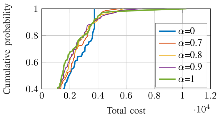
Consider the cumulative probability distribution of the total cost $\sum_{t=0}^{N-1}\ell_{t}(x_{t},u_{t},w_{t})+\ell_{N}(x_{N})$ in Fig. 4. The worst-case cost is minimal for $\alpha=0$ at the expense of a higher cost when moving away from the extremes. By contrast, for $\alpha=1$, the expected cost is minimal, yet high costs may occur with low probability. Intermediate values of $\alpha$ result in a trade-off between the two, effectively determining the extent to which the right tail of the distribution of the cost is compressed.

Figure 4: Cumulative probability distribution of the total cost after solving the risk-averse optimal control problem for different values of $\alpha$ in $\AVARa$ in absense of risk constraints.

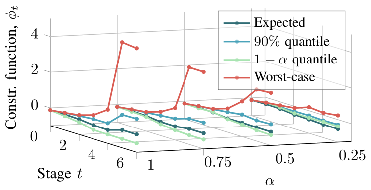
Next, consider the stage constraints function $\phi_{t}(x,u,w)=\|x\|^{2}-c$ with $c=0.5$. We use $\AVAR_{0.5}$ in the cost and impose the stage-wise risk constraint $\AVARa(\phi_{t}(x_{t},u_{t},w_{t}))\leq 0$ at all stages $t\in\N_{[N-4,N-1]}$. For the robust case ($\alpha=0$), there was no feasible solution. As $\alpha$ increases, Fig. 5 shows that constraint violations occur in larger fractions of the realisations. Also note that since $\AVARa$ bounds the $(1-\alpha)$-quantile function, it is guaranteed that $\prob[\|x_{t}\|\leq c]\geq 1-\alpha$.

Figure 5: The constraint function $\phi_{t}$ over time for a risk-averse optimal control problem with different values of $\alpha$ in the average value-at-risk.

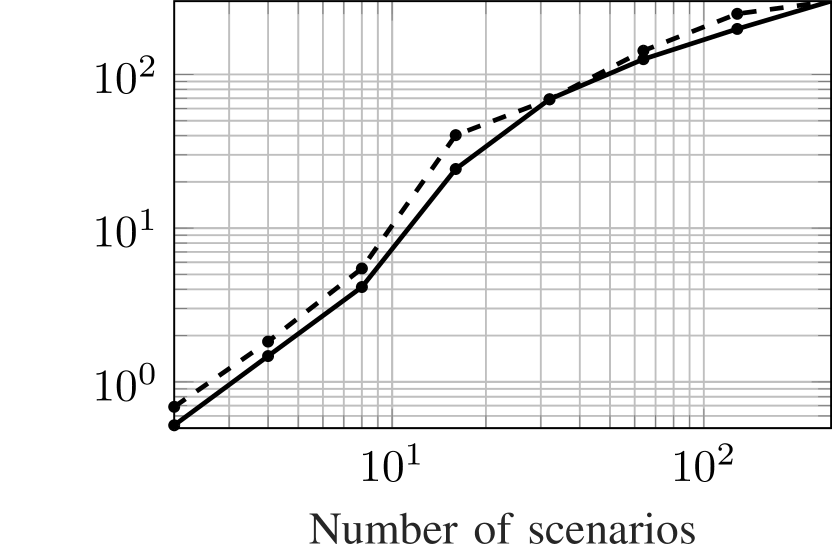
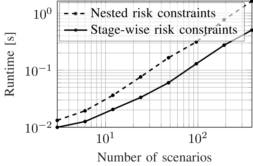
Fig. 6 shows the complexity of the optimization problem with respect to the number of scenarios. We fixed $N=12$ and controlled the number of scenarios and nodes with the branching horizon $t_{0}$. Although nested risk constraints increase the problem size, the asymptotic complexity remains linear in the number of nodes. Moreover, for both constraint types, problems using $\AVAR$ with up to 200 scenarios can still be solved in well under a second. Since MOSEK V. 8 [28] does not support exponential constraints, it cannot be used to solve problems involving $\EVAR$. For that reason, we resort to SuperSCS [29]. As shown in Fig. 6, $\EVAR$-based problems are solved at a significantly higher runtime.

Figure 6: Solver time versus the number of scenarios in the tree (computed on an Intel Core i7-7700K CPU at 4.20GHz). (left) $\AVAR$ (MOSEK [28]); (right) $\EVAR$ (SuperSCS [29]).

VII Conclusions

We presented a decomposition methodology for nested conditional risk mappings in multistage risk-averse optimal control problems. In the common case where the system dynamics is linear and the state and input constraints are convex, the original multistage nested problem is cast as a conic problem, which can be solved very efficiently and is suitable for real-time embedded applications, provided that the tree contains a moderate number of nodes. The proposed approach hinges on the convex dual formulation of conic risk measures. Future work will focus on tailored numerical methods to exploit the tree structure to solve such problems fast, efficiently and using parallelization (e.g., on GPUs [30, 31]).

Proof:

Let $\rho:\Re^{n}\rightarrow\Re$ be a convex risk measure and $g{}:{}\Re^{m}\ni x\mapsto\left(g_{1}(x),g_{2}(x),\dots,g_{n}(x)\right)\in\Re^{n}$. Define $g^{\star}=\inf_{x\in X}g(x)$; we know that $\inf_{x\in X}g_{i}(x)$ are finite because of [32, Thm. 1.9]. For $\epsilon>0$, define

$$\B_{\epsilon}^{g}=\left\{x\in X\mid g_{i}(x)\leq g_{i}^{\star}+\epsilon,i=1,\ldots,n\right\}.$$

By the definition of infimum, $\B_{\epsilon}^{g}$ are nonempty and nested ($\B_{\epsilon^{\prime}}^{g}\subseteq\B_{\epsilon}^{g}$ for $\epsilon^{\prime}\leq\epsilon$). For $x\in\B_{\epsilon}^{g}$ we have $g^{\star}\leq g(x)\leq g^{\star}+\epsilon$. Using the monotonicity property of $\rho$ (A2) we obtain

$$\rho[{}g^{\star}{}]{}\leq{}\rho[{}g(x){}],$$ (20)

for all $x\in\B_{\epsilon}^{g}$. By taking the infimum on both sides of (20) we obtain

$$\rho[{}g^{\star}{}]{}\leq{}\inf_{\epsilon>0}\inf_{x\in\B_{\epsilon}^{g}}\rho[{}g(x){}]{}={}\inf_{x\in X}\rho[{}g(x){}].$$ (21a)

Conversely, take $$x^{\epsilon}\in\B_{\epsilon}^{g} \epsilon{}\downarrow{}0 g(x^{\epsilon})\to g^{\star} \rho \rho[{}g(x^{\epsilon}){}]{}\to{}\rho[{}g^{\star}{}] \inf_{x\in X}\rho[{}g(x){}]\leq\rho[{}g(x){}]$$. As , and because is continuous, . Since ,

$$\inf_{x\in X}\rho[{}g(x){}]{}\leq{}\rho[{}g^{\star}{}].$$ (21b)

By (21a) and (21b) we have established (15a).

Let us assume now that $\operatorname*{\arg\!\min}_{x\in X}g(x)$ is a nonempty set. For any $x^{\star}\in\operatorname*{\arg\!\min}_{x\in X}g(x)$ it holds by definition that $g(x^{\star})=\inf_{x\in X}g(x)$. Then, by the property established above it holds that $\rho[{}g(x^{\star}){}]{}={}\inf_{x\in X}\rho[{}g(x){}]$, therefore, (15b) holds true.

If $\rho\circ g$ is strictly convex, then the minimizer is unique, therefore (16) holds. Assume that risk measure $\rho$ is strictly monotone (see Condition A5) and there exists $\bar{x}\in\operatorname*{\arg\!\min}_{x\in X}\rho\left(g(x)\right)$, but $\bar{x}\notin\operatorname*{\arg\!\min}_{x\in X}g(x)$. Then, $g(x^{\star})<g(\bar{x})$ which, by strict monotonicity, implies $\rho[{}g(x^{\star}){}]<\rho[{}g(\bar{x}){}]$ leading to contradiction. ∎

Proof:

For $Y_{t+1}\in\Re^{|\operatorname{nodes}(t+1)|}$ and $Y_{0}\in\Re$, we have that $(Y_{t+1},Y_{0})\in\operatorname{epi}\bar{\rho}_{t}$ if $\bar{\rho}_{t}[Y_{t+1}]\leq Y_{0}$ and using Theorem V.1

$$\bar{\rho}_{t}[Y_{t+1}]= \rho_{\mid{}0}[{}\cdots{}\rho_{\mid{}t-1}[\rho_{\mid{}t}[Y_{t+1}]]]$$

$$= \rho_{\mid{}0}\Big{[}{}\cdots{}\rho_{\mid{}t-1}\big{[}\inf_{\rho_{\mid{}t}[Y_{t+1}]\leq Y_{t}}Y_{t}\big{]}\Big{]}$$

$$= \inf_{(Y_{t+1},Y_{t})\in\operatorname{epi}\rho_{\mid{}t}}\rho_{\mid{}0}\big{[}{}\cdots{}\rho_{\mid{}t-1}[Y_{t}]\big{]}$$

$$= \inf_{(Y_{t+1},Y_{t})\in\operatorname{epi}\rho_{\mid{}t}}\bar{\rho}_{t-1}[Y_{t}]$$

repeating recursively the same procedure, proves Proposition V.2. ∎

References

• [1] A. Shapiro, D. Dentcheva, and Ruszczyński, Lectures on stochastic programming: modeling and theory. SIAM, 2nd ed., 2014.
• [2] G. Pflug and W. Römisch, Modeling, Measuring and Managing Risk. World Scientific, 2007.
• [3] G. C. Calafiore and L. E. Ghaoui, “On distributionally robust chance-constrained linear programs,” Journal of Optimization Theory and Applications, vol. 130, no. 1, pp. 1–22, 2006.
• [4] D. Bertsimas and D. B. Brown, “Constructing uncertainty sets for robust linear optimization,” Oper. Res., vol. 57(6), pp. 1483–95, 2009.
• [5] A. Ben-Tal, D. Bertsimas, and D. B. Brown, “A soft robust model for optimization under ambiguity,” Oper. Res., vol. 58, no. 4-part-2, pp. 1220–1234, 2010.
• [6] A. Nemirovski and A. Shapiro, “Convex approximations of chance constrained programs,” SIAM J. Optim., vol. 17, pp. 969–96, Dec 2006.
• [7] A. Nemirovski, “On safe tractable approximations of chance constraints,” Eur. J. Oper. Res., vol. 219, no. 3, pp. 707 – 718, 2012. Feature Clusters.
• [8] Y. Chow and M. Ghavamzadeh, “Algorithms for CVaR optimization in MDPs,” in NIPS, pp. 3509–3517, 2014.
• [9] S. Shen, “Using integer programming for balancing return and risk in problems with individual chance constraints,” Computers & Operations Research, vol. 49, pp. 59 – 70, 2014.
• [10] C. A. Hans, P. Sopasakis, J. Raisch, C. Reincke-Collon, and P. Patrinos, “Risk-averse model predictive operation control of islanded microgrids,” ArXiv e-prints, 2018. https://arxiv.org/abs/1809.06062.
• [11] T. Asamov and A. Ruszczyński, “Time-consistent approximations of risk-averse multistage stochastic optimization problems,” Math. Prog., vol. 153, no. 2, pp. 459–493, 2015.
• [12] R. A. Collado, D. Papp, and A. Ruszczyński, “Scenario decomposition of risk-averse multistage stochastic programming problems,” Ann. Oper. Res., vol. 200, pp. 147–170, 2012.
• [13] S. Bruno, S. Ahmed, A. Shapiro, and S. Stree, “Risk neutral and risk averse approaches to multistage renewable investment planning under uncertainty,” Eur. J. Oper. Res., vol. 250, no. 3, pp. 979 – 989, 2016.
• [14] P. Patrinos and H. Sarimveis, “An explicit optimal control approach for mean-risk dynamic portfolio allocation,” in ECC, 2007.
• [15] R. T. Rockafellar and S. Uryasev, “Optimization of conditional value-at-risk,” Journal of Risk, vol. 2, pp. 21–41, 2000.
• [16] R. Collado, S. Meisel, and L. Priekule, “Risk-averse stochastic path detection,” Eur. J. Oper. Res., vol. 260, no. 1, pp. 195 – 211, 2017.
• [17] A. Ahmadi-Javid and M. Fallah-Tafti, “Portfolio optimization with entropic value-at-risk,” ArXiv e-prints, 08 2017.
• [18] A. Shapiro and A. Pichler, “Time and dynamic consistency of risk averse stochastic programs,” Optimization Online, 2016. Available at http://www.optimization-online.org/DB_HTML/2016/09/5654.html.
• [19] A. Ahmadi-Javid, “Entropic value-at-risk: A new coherent risk measure,” J. Optim. Theory & Appl., vol. 155, no. 3, pp. 1105–1123, 2012.
• [20] G. Pflug and A. Pichler, “Dynamic generation of scenario trees,” Comput. Optimization Appl., vol. 62, no. 3, pp. 641–668, 2015.
• [21] H. Heitsch and W. Römisch, “Scenario tree modeling for multistage stochastic programs,” Math. Prog., vol. 118, no. 2, pp. 371–406, 2009.
• [22] D. P. Bertsekas, Dynamic Programming and Optimal Control, vol. I. Athena Scientific, 4th ed., 2012.
• [23] Y.-L. Chow and M. Pavone, “A framework for time-consistent, risk-averse model predictive control: Theory and algorithms,” in ACC, pp. 4204 – 4211, 2014.
• [24] P. Sopasakis, D. Herceg, A. Bemporad, and P. Patrinos, “Risk-averse model predictive control,” Automatica, vol. 100, 2019.
• [25] R. Rockafellar and S. Uryasev, “The fundamental risk quadrangle in risk management, optimization and statistical estimation,” Surv. Oper. Res. & Manag. Sci., vol. 18, pp. 33–53, 2013.
• [26] A. Ben-Tal, L. El Ghaoui, and A. Nemirovski, Robust Optimization. Princeton Series in Applied Mathematics, Princeton Univ. Press, 2009.
• [27] A. Ben-Tal and A. Nemirovski, Lectures on Modern Convex Optimization. Society for Industrial and Applied Mathematics, jan 2001.
• [28] MOSEK ApS, The MOSEK optimization toolbox for MATLAB manual. Version 8.1., 2017.
• [29] P. Sopasakis, K. Menounou, and P. Patrinos, “SuperSCS: fast and accurate large-scale conic optimization,” in ECC, 2019.
• [30] A. Sampathirao, P. Sopasakis, A. Bemporad, and P. Patrinos, “GPU-accelerated stochastic predictive control of drinking water networks,” IEEE TCST, vol. 26, no. 2, 2018.
• [31] A. Sampathirao, P. Sopasakis, A. Bemporad, and P. Patrinos, “Distributed solution of stochastic optimal control problems on GPUs,” in IEEE CDC, 2015.
• [32] R. T. Rockafellar and R. J.-B. Wets, Variational analysis, vol. 317. Springer, 2011.
Proof:
Let ρ:n:𝜌superscript𝑛\rho:\Re^{n}\rightarrow\Re be a convex risk measure and g:mx(g1(x),g2(x),,gn(x))n:𝑔containssuperscript𝑚𝑥maps-tosubscript𝑔1𝑥subscript𝑔2𝑥subscript𝑔𝑛𝑥superscript𝑛g{}:{}\Re^{m}\ni x\mapsto\left(g_{1}(x),g_{2}(x),\dots,g_{n}(x)\right)\in\Re^{n}. Define g=infxXg(x)superscript𝑔subscriptinfimum𝑥𝑋𝑔𝑥g^{\star}=\inf_{x\in X}g(x); we know that infxXgi(x)subscriptinfimum𝑥𝑋subscript𝑔𝑖𝑥\inf_{x\in X}g_{i}(x) are finite because of [32, Thm. 1.9]. For ϵ>0italic-ϵ0\epsilon>0, define
\Bϵg={xXgi(x)gi+ϵ,i=1,,n}.superscriptsubscript\Bitalic-ϵ𝑔conditional-set𝑥𝑋formulae-sequencesubscript𝑔𝑖𝑥superscriptsubscript𝑔𝑖italic-ϵ𝑖1𝑛\B_{\epsilon}^{g}=\left\{x\in X\mid g_{i}(x)\leq g_{i}^{\star}+\epsilon,i=1,\ldots,n\right\}.
By the definition of infimum, \Bϵgsuperscriptsubscript\Bitalic-ϵ𝑔\B_{\epsilon}^{g} are nonempty and nested (\Bϵg\Bϵgsuperscriptsubscript\Bsuperscriptitalic-ϵ𝑔superscriptsubscript\Bitalic-ϵ𝑔\B_{\epsilon^{\prime}}^{g}\subseteq\B_{\epsilon}^{g} for ϵϵsuperscriptitalic-ϵitalic-ϵ\epsilon^{\prime}\leq\epsilon). For x\Bϵg𝑥superscriptsubscript\Bitalic-ϵ𝑔x\in\B_{\epsilon}^{g} we have gg(x)g+ϵsuperscript𝑔𝑔𝑥superscript𝑔italic-ϵg^{\star}\leq g(x)\leq g^{\star}+\epsilon. Using the monotonicity property of ρ𝜌\rho (A2) we obtain
ρ[g]ρ[g(x)],𝜌delimited-[]superscript𝑔𝜌delimited-[]𝑔𝑥\displaystyle\rho[{}g^{\star}{}]{}\leq{}\rho[{}g(x){}], (20)
for all x\Bϵg𝑥superscriptsubscript\Bitalic-ϵ𝑔x\in\B_{\epsilon}^{g}. By taking the infimum on both sides of (20) we obtain
ρ[g]infϵ>0infx\Bϵgρ[g(x)]=infxXρ[g(x)].𝜌delimited-[]superscript𝑔subscriptinfimumitalic-ϵ0subscriptinfimum𝑥superscriptsubscript\Bitalic-ϵ𝑔𝜌delimited-[]𝑔𝑥subscriptinfimum𝑥𝑋𝜌delimited-[]𝑔𝑥\displaystyle\rho[{}g^{\star}{}]{}\leq{}\inf_{\epsilon>0}\inf_{x\in\B_{\epsilon}^{g}}\rho[{}g(x){}]{}={}\inf_{x\in X}\rho[{}g(x){}]. (21a)
Conversely, take xϵ\Bϵgsuperscript𝑥italic-ϵsuperscriptsubscript\Bitalic-ϵ𝑔x^{\epsilon}\in\B_{\epsilon}^{g}. As ϵ0italic-ϵ0\epsilon{}\downarrow{}0, g(xϵ)g𝑔superscript𝑥italic-ϵsuperscript𝑔g(x^{\epsilon})\to g^{\star} and because ρ𝜌\rho is continuous, ρ[g(xϵ)]ρ[g]𝜌delimited-[]𝑔superscript𝑥italic-ϵ𝜌delimited-[]superscript𝑔\rho[{}g(x^{\epsilon}){}]{}\to{}\rho[{}g^{\star}{}]. Since infxXρ[g(x)]ρ[g(x)]subscriptinfimum𝑥𝑋𝜌delimited-[]𝑔𝑥𝜌delimited-[]𝑔𝑥\inf_{x\in X}\rho[{}g(x){}]\leq\rho[{}g(x){}],
infxXρ[g(x)]ρ[g].subscriptinfimum𝑥𝑋𝜌delimited-[]𝑔𝑥𝜌delimited-[]superscript𝑔\inf_{x\in X}\rho[{}g(x){}]{}\leq{}\rho[{}g^{\star}{}]. (21b)