\emails

lu_lu@mit.edu (L. Lu), yeonjong_shin@brown.edu (Y. Shin), suyh@fzu.edu.cn (Y. Su), george_karniadakis@brown.edu (G. E. Karniadakis). L. Lu and Y. Shin contributed equally to this work.

Dying ReLU and Initialization: Theory and Numerical Examples

Lu Lu 1    Yeonjong Shin\comma\corrauth 2    Yanhui Su 3    and George Em Karniadakis 2 11affiliationmark:  Department of Mathematics, Massachusetts Institute of Technology, Cambridge, MA 02139, USA
22affiliationmark:  Division of Applied Mathematics, Brown University, Providence, RI 02912, USA
33affiliationmark:  College of Mathematics and Computer Science, Fuzhou University, Fuzhou, Fujian 350116, China
Abstract

The dying ReLU refers to the problem when ReLU neurons become inactive and only output 0 for any input. There are many empirical and heuristic explanations of why ReLU neurons die. However, little is known about its theoretical analysis. In this paper, we rigorously prove that a deep ReLU network will eventually die in probability as the depth goes to infinite. Several methods have been proposed to alleviate the dying ReLU. Perhaps, one of the simplest treatments is to modify the initialization procedure. One common way of initializing weights and biases uses symmetric probability distributions, which suffers from the dying ReLU. We thus propose a new initialization procedure, namely, a randomized asymmetric initialization. We show that the new initialization can effectively prevent the dying ReLU. All parameters required for the new initialization are theoretically designed. Numerical examples are provided to demonstrate the effectiveness of the new initialization procedure.

keywords:
Neural network, Dying ReLU, Vanishing/Exploding gradient, Randomized asymmetric initialization.
\ams

60J05, 62M45, 68U99

1 Introduction

The rectified linear unit (ReLU), max{x,0}𝑥0\max\{x,0\}, is one of the most successful and widely-used activation functions in deep learning [30, 40, 35]. The success of ReLU is based on its superior training performance [16, 47] over other activation functions such as the logistic sigmoid and the hyperbolic tangent [15, 31]. The ReLU has been used in various applications including image classification [29, 49], natural language processes [33], speech recognition [23], and game intelligence [44], to name a few.

The use of gradient-based optimization is inevitable in training deep neural networks. It has been widely known that the deeper a neural network is, the harder it is to train [46, 9]. A fundamental difficulty in training deep neural networks is the vanishing and exploding gradient problem [39, 17, 6]. The dying ReLU is a kind of vanishing gradient, which refers to a problem when ReLU neurons become inactive and only output 0 for any input. It has been known as one of the obstacles in training deep feed-forward ReLU neural networks [50, 1]. To overcome this problem, a number of methods have been proposed. Broadly speaking, these can be categorized into three general approaches. One approach modifies the network architectures. This includes but not limited to the changes in the number of layers, the number of neurons, network connections, and activation functions. In particular, many activation functions have been proposed to replace the ReLU [33, 20, 7, 28]. However, the performance of other activation functions varies on different tasks and data sets [40] and it typically requires a parameter to be turned. Thus, the ReLU remains one of the popular activation functions due to its simplicity and reliability. Another approach introduces additional training steps. This includes several normalization techniques [24, 42, 51, 4, 53] and dropout [45]. One of the most successful normalization techniques is the batch normalization [24]. It is a technique that inserts layers into the deep neural network that transform the output for the batch to be zero mean unit variance. However, batch normalization increases by 30% the computational overhead to each iteration [34]. The third approach modifies only weights and biases initialization procedure without changing any network architectures or introducing additional training steps [31, 15, 20, 43, 34]. The third approach is the topic of our work presented in this paper.

The intriguing ability of gradient-based optimization is perhaps one of the major contributors to the success of deep learning. Training deep neural networks using gradient-based optimization fall into the noncovex nonsmooth optimization. Since a gradient-based method is either a first- or a second-order method, and once converged, the optimizer is either a local minimum or a saddle point. The authors of [12] proved that the existence of local minima poses a serious problem in training neural networks. Many researchers have been putting immense efforts to mathematically understand the gradient method and its ability to solve nonconvex nonsmooth problems. Under various assumptions, especially on the landscape, many results claim that the gradient method can find a global minimum, can escape saddle points, and can avoid spurious local minima [32, 2, 13, 14, 57, 52, 55, 8, 10, 9, 25]. However, these assumptions do not always hold and are provably false for deep neural networks [41, 26, 3]. This further limits our understanding on what contributes to the success of the deep neural networks. Often, theoretical conditions are impossible to be met in practice.

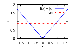
Where to start the optimization process plays a critical role in training and has a significant effect on the trained result [36]. This paper focuses on a particular kind of bad local minima due to a bad initialization. Such a bad local minimum causes the dying ReLU. Specifically, we consider the worst case of dying ReLU, where the entire network dies, i.e., the network becomes a constant function. We refer this as the dying ReLU neural networks (NNs). This phenomenon could be well illustrated by a simple example. Suppose f(x)=|x|𝑓𝑥𝑥f(x)=|x| is a target function we want to approximate using a ReLU network. Since |x|=ReLU(x)+ReLU(x)𝑥ReLU𝑥ReLU𝑥|x|=\text{ReLU}(x)+\text{ReLU}(-x), a 2-layer ReLU network of width 2 can exactly represent |x|𝑥|x|. However, when we train a deep ReLU network, we frequently observe that the network is collapsed. This trained result is shown in Fig. 1. Our 1,000 independent simulations show that there is a high probability (more than 90%) for the deep ReLU network to collapse to a constant function. In this example, we employ a 10-layer ReLU network of width 2 which should perfectly recover f(x)=|x|𝑓𝑥𝑥f(x)=|x|.

Refer to caption
Figure 1: An approximation result for f(x)=|x|𝑓𝑥𝑥f(x)=|x| using a 10-layer ReLU neural network of width 2. Among 1,000 independent simulations, this trained result is obtained with more than 90% probability. One of the most popular initialization procedures [20] is employed.

Almost all common initialization schemes in training deep neural networks use symmetric probability distributions around 0. For example, zero mean uniform distributions and zero mean normal distributions were proposed and used in [31, 15, 20]. We show that when weights and biases are initialized from symmetric probability distributions around 0, the dying ReLU NNs occurs in probability as the number of depth goes to infinite. To the best of our knowledge, this is the first theoretical work on the dying ReLU. This result partially explains why training extremely deep networks is challenging. Furthermore, it says that the dying ReLU is inevitable as long as the network is deep enough. Also, our result implies that it is the network architecture that decides whether an initialization procedure is good or bad. Our analysis reveals that a specific network architecture can avoid the dying ReLU NNs with high probability. That is, for any δ>0𝛿0\delta>0, when a symmetric initialization is used and L=Ω(log2(N/δ))𝐿Ωsubscript2𝑁𝛿L=\Omega(\log_{2}(N/\delta)) is satisfied where L𝐿L is the number of depth and N𝑁N is the number of width at each layer, with probability 1δ1𝛿1-\delta, the dying ReLU NNs will not happen. This explains why wide networks are popularly used in practice. However, the use of deep and wide networks requires one to train a gigantic number of parameters and this could be computationally very expensive and time consuming.

On the other hands, deep and narrow networks play fundamental roles both in theory and in practice. For example, in the work of [19], it was shown that deep and narrow ReLU networks are inevitable in constructing finite element’s basis functions. This represents an application of deep ReLU networks in finite element method for solving PDEs. Also, many theoretical works [38, 54, 18] on the expressivity of ReLU networks rely heavily on deep and narrow networks in approximating polynomials through sparse concatenations. Despite the importance of deep and narrow networks, due to aforementioned reasons, they have not been successfully employed in practice. Thereby, we propose an initialization scheme, namely, a randomized asymmetric initialization (RAI), to directly overcome the dying ReLU. On the theoretical side, we show that RAI has a smaller upper bound of the probability of the dying ReLU NNs than standard symmetric initialization such as the He initialization [20]. All hyper-parameters for RAI are theoretically driven to avoid the exploding gradient problem. This is done by the second moment analysis [20, 17, 39].

The rest of the paper is organized as follows. After setting up notation and terminology in Section 2, we present the main theoretical results in Section 3. In Section 4, upon introducing a randomized asymmetric initialization, we discuss its theoretical properties. Numerical examples are provided in Section 5, before the conclusion in Section 6.

2 Mathematical setup

Let 𝒩L:dindout:superscript𝒩𝐿superscriptsubscript𝑑insuperscriptsubscript𝑑out\mathcal{N}^{L}:\mathbb{R}^{d_{\text{in}}}\to\mathbb{R}^{d_{\text{out}}} be a feed-forward neural network with L𝐿L layers and Nsubscript𝑁N_{\ell} neurons in the \ell-th layer (N0=dinsubscript𝑁0subscript𝑑inN_{0}=d_{\text{in}}, NL=doutsubscript𝑁𝐿subscript𝑑outN_{L}=d_{\text{out}}). Let us denote the weight matrix and bias vector in the \ell-th layer by 𝑾𝐑N×N1superscript𝑾superscript𝐑subscript𝑁subscript𝑁1\bm{W}^{\ell}\in\mathbf{R}^{N_{\ell}\times N_{\ell-1}} and 𝐛Nsuperscript𝐛superscriptsubscript𝑁\mathbf{b}^{\ell}\in\mathbb{R}^{N_{\ell}}, respectively. Given an activation function ϕitalic-ϕ\phi which is applied element-wise, the feed-forward neural network is recursively defined as follows: 𝒩1(x)=𝑾1x+𝒃1superscript𝒩1xsuperscript𝑾1xsuperscript𝒃1\mathcal{N}^{1}(\textbf{x})=\bm{W}^{1}\textbf{x}+\bm{b}^{1} and

𝒩(x)superscript𝒩x\displaystyle\mathcal{N}^{\ell}(\textbf{x}) =𝑾ϕ(𝒩1(x))+𝒃N,for2L.formulae-sequenceabsentsuperscript𝑾italic-ϕsuperscript𝒩1xsuperscript𝒃superscriptsubscript𝑁for2𝐿\displaystyle=\bm{W}^{\ell}\phi(\mathcal{N}^{\ell-1}(\textbf{x}))+\bm{b}^{\ell}\in\mathbb{R}^{N_{\ell}},\qquad\text{for}\quad 2\leq\ell\leq L. (1)

Here 𝒩Lsuperscript𝒩𝐿\mathcal{N}^{L} is called a L𝐿L-layer neural network or a (L1)𝐿1(L-1)-hidden layer neural network. In this paper, the rectified linear unit (ReLU) activation function is employed, i.e.,

ϕ(x)=ReLU(x):=(max{x1,0},,max{xfan-in,0}),wherex=(x1,,xfan-in).formulae-sequenceitalic-ϕxReLUxassignsubscript𝑥10subscript𝑥fan-in0wherexsubscript𝑥1subscript𝑥fan-in\phi(\textbf{x})=\text{ReLU}(\textbf{x}):=\left(\max\{x_{1},0\},\cdots,\max\{x_{\text{fan-in}},0\}\right),\quad\text{where}\quad\textbf{x}=(x_{1},\cdots,x_{\text{fan-in}}).

Let 𝑵=(N0,N1,,NL)𝑵subscript𝑁0subscript𝑁1subscript𝑁𝐿\vec{\bm{N}}=(N_{0},N_{1},\cdots,N_{L}) be a vector representing the network architecture. Let 𝜽𝑵={𝑾,𝒃}1Lsubscript𝜽𝑵subscriptsuperscript𝑾superscript𝒃1𝐿\bm{\theta}_{\vec{\bm{N}}}=\{\bm{W}^{\ell},\bm{b}^{\ell}\}_{1\leq\ell\leq L} be the set of all weight matrices and bias vectors. Let 𝒯m={xi,yi}1imsubscript𝒯𝑚subscriptsubscriptx𝑖subscript𝑦𝑖1𝑖𝑚\mathcal{T}_{m}=\{\textbf{x}_{i},y_{i}\}_{1\leq i\leq m} be the set of m𝑚m training data and let 𝒟={xi}i=1m𝒟superscriptsubscriptsubscriptx𝑖𝑖1𝑚\mathcal{D}=\{\textbf{x}_{i}\}_{i=1}^{m} be the training input data. We assume that 𝒟Br(0)𝒟subscript𝐵𝑟0\mathcal{D}\subset B_{r}(0) for some r>0𝑟0r>0. Given 𝒯msubscript𝒯𝑚\mathcal{T}_{m}, in order to train 𝜽𝑵subscript𝜽𝑵\bm{\theta}_{\vec{\bm{N}}}, we consider the standard loss function (𝜽𝑵,𝒯m)subscript𝜽𝑵subscript𝒯𝑚\mathcal{L}(\bm{\theta}_{\vec{\bm{N}}},\mathcal{T}_{m}):

(𝜽𝑵,𝒯m)=1m(x,y)𝒯m(𝒩L(x;𝜽𝑵),y),subscript𝜽𝑵subscript𝒯𝑚1𝑚subscriptx𝑦subscript𝒯𝑚superscript𝒩𝐿xsubscript𝜽𝑵𝑦\mathcal{L}(\bm{\theta}_{\vec{\bm{N}}},\mathcal{T}_{m})=\frac{1}{m}\sum_{(\textbf{x},y)\in\mathcal{T}_{m}}\ell(\mathcal{N}^{L}(\textbf{x};\bm{\theta}_{\vec{\bm{N}}}),y), (2)

where :dout×dout:superscriptsubscript𝑑outsuperscriptsubscript𝑑out\ell:\mathbb{R}^{d_{\text{out}}}\times\mathbb{R}^{d_{\text{out}}}\to\mathbb{R} is a loss criterion. In training neural networks, the gradient-based optimization is typically employed to minimize the loss \mathcal{L}. The first step for training would be to initialize weight matrices and bias vectors. Typically, they are initialized according to certain probability distributions. For example, uniform distributions around 0 or zero-mean normal distributions are common choices.

In this paper, we focus on the worst case of dying ReLU, where the entire network dies, i.e., the network becomes a constant function. We refer this as the dying ReLU neural network. We then define two phases: (1) a network is dead before training, and (2) a network is dead after training. The phase 1 implies the phase 2, but not vice versa. When the phase 1 happens, we say the network is born dead (BD).

3 Dying probability bounds and asymptotic properties

We investigate the probability of the dying ReLU neural networks at random initialization. Let (Ω,,P)Ω𝑃(\Omega,\mathcal{F},P) be a probability space. For a network architecture 𝑵L=(din,N1,,NL1,dout)subscript𝑵𝐿subscript𝑑insubscript𝑁1subscript𝑁𝐿1subscript𝑑out\vec{\bm{N}}_{L}=(d_{\text{in}},N_{1},\cdots,N_{L-1},d_{\text{out}}), let 𝜽𝑵L:Ω|𝑵L|:subscript𝜽subscript𝑵𝐿Ωsuperscriptsubscript𝑵𝐿\bm{\theta}_{\vec{\bm{N}}_{L}}:\Omega\to\mathbb{R}^{|\vec{\bm{N}}_{L}|} be a vector-valued random variable, where |𝑵L|:==1LN(N1+1)assignsubscript𝑵𝐿superscriptsubscript1𝐿subscript𝑁subscript𝑁11|\vec{\bm{N}}_{L}|:=\sum_{\ell=1}^{L}N_{\ell}(N_{\ell-1}+1) is the total number of network parameters. Let us consider the following BD event:

𝔍𝑵L:={ωΩ|𝒩L(x;𝜽𝑵L(ω)) is a constant function in 𝒟}.assignsubscript𝔍subscript𝑵𝐿conditional-set𝜔Ωsuperscript𝒩𝐿xsubscript𝜽subscript𝑵𝐿𝜔 is a constant function in 𝒟\mathfrak{J}_{\vec{\bm{N}}_{L}}:=\{\omega\in\Omega\hskip 2.84544pt|\hskip 2.84544pt\mathcal{N}^{L}(\textbf{x};\bm{\theta}_{\vec{\bm{N}}_{L}}(\omega))\text{ is a constant function in }\mathcal{D}\}. (3)

Then, P(𝔍𝑵L)𝑃subscript𝔍subscript𝑵𝐿P(\mathfrak{J}_{\vec{\bm{N}}_{L}}) is the BD probability (BDP). The following theorem shows that a deep ReLU network will eventually be BD in probability as the number of depth L𝐿L goes to infinity.

Theorem 3.1.

For 𝐍L=(din,N,,N,dout)L+1subscript𝐍𝐿subscript𝑑in𝑁𝑁subscript𝑑outsuperscript𝐿1\vec{\bm{N}}_{L}=(d_{\text{in}},N,\cdots,N,d_{\text{out}})\in\mathbb{N}^{L+1}, let 𝛉𝐍L={𝐖,𝐛}1Lsubscript𝛉subscript𝐍𝐿subscriptsuperscript𝐖superscript𝐛1𝐿\bm{\theta}_{\vec{\bm{N}}_{L}}=\{\bm{W}^{\ell},\bm{b}^{\ell}\}_{1\leq\ell\leq L} and 𝒩L(x;𝛉𝐍L)superscript𝒩𝐿xsubscript𝛉subscript𝐍𝐿\mathcal{N}^{L}(\textbf{x};\bm{\theta}_{\vec{\bm{N}}_{L}}) be a ReLU neural network with L𝐿L layers, each having N𝑁N neurons. Suppose that all weights and biases are randomly initialized from probability distributions, which satisfy

P(𝑾jN1,𝒃j<0)p>0,1jN,1L,formulae-sequence𝑃formulae-sequencesubscriptsuperscript𝑾𝑗subscriptsuperscriptsubscript𝑁1subscriptsuperscript𝒃𝑗0𝑝0for-all1𝑗subscript𝑁for-all1𝐿P\left(\bm{W}^{\ell}_{j}\in\mathbb{R}^{N_{\ell-1}}_{-},\bm{b}^{\ell}_{j}<0\right)\geq p>0,\qquad\forall 1\leq j\leq N_{\ell},\forall 1\leq\ell\leq L, (4)

for some constant p>0𝑝0p>0, where 𝐖jsubscriptsuperscript𝐖𝑗\bm{W}^{\ell}_{j} is the j𝑗j-th row of the \ell-th layer weight matrix and 𝐛jsubscriptsuperscript𝐛𝑗\bm{b}^{\ell}_{j} is the j𝑗j-th component of the \ell-th layer bias vector. Then

limLP(𝔍𝑵L)=1,subscript𝐿𝑃subscript𝔍subscript𝑵𝐿1\begin{split}\lim_{L\to\infty}P(\mathfrak{J}_{\vec{\bm{N}}_{L}})=1,\end{split}

where 𝔍𝐍Lsubscript𝔍subscript𝐍𝐿\mathfrak{J}_{\vec{\bm{N}}_{L}} is defined in (3).

Proof 3.2.

The proof can be found in Appendix A.

We remark that Equation 4 is a very mild condition and it can be satisfied in many cases. For example, when symmetric probability distributions around 0 are employed, the condition is met with p=2N1𝑝superscript2𝑁1p=2^{-N-1}. Theorem 3.1 implies that the fully connected ReLU network will be dead at the initialization as long as the network is deep enough. This explains theoretically why training a very deep network is hard.

Theorem 3.1 shows that the ReLU network asymptotically will be dead. Thus, we are now concerned with the convergence behavior of the probability of NNs being BD. Since almost all common initialization procedures use symmetric probability distributions around 0, we derive an upper bound of the born dead probability (BDP) for symmetric initialization.

Theorem 3.3.

For 𝐍L=(din,N1,,NL1,dout)L+1subscript𝐍𝐿subscript𝑑insubscript𝑁1subscript𝑁𝐿1subscript𝑑outsuperscript𝐿1\vec{\bm{N}}_{L}=(d_{\text{in}},N_{1},\cdots,N_{L-1},d_{\text{out}})\in\mathbb{N}^{L+1}, let 𝛉𝐍L={𝐖,𝐛}1Lsubscript𝛉subscript𝐍𝐿subscriptsuperscript𝐖superscript𝐛1𝐿\bm{\theta}_{\vec{\bm{N}}_{L}}=\{\bm{W}^{\ell},\bm{b}^{\ell}\}_{1\leq\ell\leq L} and 𝒩L(x;𝛉𝐍L)superscript𝒩𝐿xsubscript𝛉subscript𝐍𝐿\mathcal{N}^{L}(\textbf{x};\bm{\theta}_{\vec{\bm{N}}_{L}}) be a ReLU neural network with L𝐿L layers, each having N1,,NL1subscript𝑁1subscript𝑁𝐿1N_{1},\cdots,N_{L-1} neurons. Suppose that all weights are independently initialized from symmetric probability distributions around 0 and all biases are either drawn from a symmetric distribution or set to zero. Then

P(𝔍𝑵L)1=1L1(1(1/2)N),𝑃subscript𝔍subscript𝑵𝐿1superscriptsubscriptproduct1𝐿11superscript12subscript𝑁P(\mathfrak{J}_{\vec{\bm{N}}_{L}})\leq 1-\prod_{\ell=1}^{L-1}(1-(1/2)^{N_{\ell}}), (5)

where 𝔍𝐍Lsubscript𝔍subscript𝐍𝐿\mathfrak{J}_{\vec{\bm{N}}_{L}} is defined in (3). Furthermore, if 𝐍L=(din,N,,N,dout)L+1subscript𝐍𝐿subscript𝑑in𝑁𝑁subscript𝑑outsuperscript𝐿1\vec{\bm{N}}_{L}=(d_{\text{in}},N,\cdots,N,d_{\text{out}})\in\mathbb{N}^{L+1},

limLP(𝔍𝑵L)=1,limNP(𝔍𝑵L)=0.\begin{split}\lim_{L\to\infty}P(\mathfrak{J}_{\vec{\bm{N}}_{L}})=1,\qquad\lim_{N\to\infty}P(\mathfrak{J}_{\vec{\bm{N}}_{L}})=0.\end{split}
Proof 3.4.

The proof can be found in Appendix B.

Theorem 3.3 provides an upper bound of the BDP. It shows that at a fixed depth L𝐿L, the network will not be BD in probability as the number of width N𝑁N goes to infinite. In order to understand how this probability behaves with respect to the number of width and depth, a lower bound is needed. We thus provide a lower bound of the BDP of ReLU NNs at din=1subscript𝑑in1d_{\text{in}}=1.

Theorem 3.5.

For a network architecture 𝐍L=(1,N,,N,dout)L+1subscript𝐍𝐿1𝑁𝑁subscript𝑑outsuperscript𝐿1\vec{\bm{N}}_{L}=(1,N,\cdots,N,d_{\text{out}})\in\mathbb{N}^{L+1}, let 𝛉𝐍L={𝐖,𝐛}1Lsubscript𝛉subscript𝐍𝐿subscriptsuperscript𝐖superscript𝐛1𝐿\bm{\theta}_{\vec{\bm{N}}_{L}}=\{\bm{W}^{\ell},\bm{b}^{\ell}\}_{1\leq\ell\leq L} and 𝒩L(x;𝛉𝐍L)superscript𝒩𝐿xsubscript𝛉subscript𝐍𝐿\mathcal{N}^{L}(\textbf{x};\bm{\theta}_{\vec{\bm{N}}_{L}}) be a ReLU neural network with L𝐿L layers, each having N𝑁N neurons. Suppose that all weights are independently initialized from continuous symmetric probability distributions around 0, which satisfies

P(𝑾j,𝒗1>0,𝑾j,𝒗2<0|𝒗1,𝒗2)14,𝟎𝒗1,𝒗2+N1,1jN,formulae-sequence𝑃superscriptsubscript𝑾𝑗subscript𝒗10superscriptsubscript𝑾𝑗subscript𝒗2bra0subscript𝒗1subscript𝒗214formulae-sequence0subscript𝒗1formulae-sequencesubscript𝒗2superscriptsubscriptsubscript𝑁1for-all1𝑗subscript𝑁\displaystyle P(\langle\bm{W}_{j}^{\ell},\bm{v}_{1}\rangle>0,\langle\bm{W}_{j}^{\ell},\bm{v}_{2}\rangle<0|\bm{v}_{1},\bm{v}_{2})\leq\frac{1}{4},\quad\bm{0}\neq\bm{v}_{1},\bm{v}_{2}\in\mathbb{R}_{+}^{N_{\ell-1}},\quad\forall 1\leq j\leq N_{\ell},

where 𝐖jsuperscriptsubscript𝐖𝑗\bm{W}_{j}^{\ell} is the j𝑗j-th row of the \ell-th layer weight matrix, and all biases are initialized to zero. Then

plow(L,N)P(𝔍𝑵L)1=1L1(1(1/2)N),subscript𝑝low𝐿𝑁𝑃subscript𝔍subscript𝑵𝐿1superscriptsubscriptproduct1𝐿11superscript12𝑁p_{\text{low}}(L,N)\leq P(\mathfrak{J}_{\vec{\bm{N}}_{L}})\leq 1-\prod_{\ell=1}^{L-1}(1-(1/2)^{N}),

where 𝔍𝐍Lsubscript𝔍subscript𝐍𝐿\mathfrak{J}_{\vec{\bm{N}}_{L}} is defined in (3), a1=1(1/2)Nsubscript𝑎11superscript12𝑁a_{1}=1-(1/2)^{N}, a2=1(1/2)N1(N1)(1/4)Nsubscript𝑎21superscript12𝑁1𝑁1superscript14𝑁a_{2}=1-(1/2)^{N-1}-(N-1)(1/4)^{N}, and

plow(L,N)=1a1L2+(12N+1)(12N)1+(N1)2N(a1L2+a2L2).subscript𝑝low𝐿𝑁1superscriptsubscript𝑎1𝐿21superscript2𝑁11superscript2𝑁1𝑁1superscript2𝑁superscriptsubscript𝑎1𝐿2superscriptsubscript𝑎2𝐿2p_{\text{low}}(L,N)=1-a_{1}^{L-2}+\frac{(1-2^{-N+1})(1-2^{-N})}{1+(N-1)2^{-N}}(-a_{1}^{L-2}+a_{2}^{L-2}).
Proof 3.6.

The proof can be found in Appendix C.

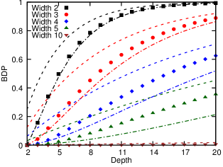
Theorem 3.5 reveals that the BDP behavior depends on the network architecture. In Fig. 2, we plot the BDP with respect to increasing the number of layers at varying width from N=2𝑁2N=2 to N=5𝑁5N=5. A bias-free ReLU feed-forward NN with din=1subscript𝑑in1d_{\text{in}}=1 is employed with weights randomly initialized from symmetric distributions. The results of one million independent simulations are used to calculate each probability estimation. Numerical estimations are shown as symbols. The upper and lower bounds from Theorem 3.5 are also plotted with dash and dash-dot lines, respectively. We see that when the NN gets narrower, the probability of NN being BD grows faster as the depth increases. Also, at a fixed width N𝑁N, the BDP grows as the number of layer increases. This is expected by Theorems 3.1 and 3.5.
Refer to caption
Figure 2: Probability of a ReLU NN to be born dead as a function of the number of layers for different widths. The dash lines represent the upper and lower bounds from Theorem 3.5. The symbols represent our numerical estimations. Similar colors correspond to the same width.

Once the network is BD, we have no hope to train the network successfully. Here we provide a formal statement of the consequence of the network being BD.

Theorem 3.7.

For any 𝐍Lsubscript𝐍𝐿\vec{\bm{N}}_{L}, suppose 𝛉𝐍Lsubscript𝛉subscript𝐍𝐿\bm{\theta}_{\vec{\bm{N}}_{L}} is initialized to be in 𝔍𝐍Lsubscript𝔍subscript𝐍𝐿\mathfrak{J}_{\vec{\bm{N}}_{L}} defined in (3). Then, for any loss function \mathcal{L}, and for any gradient based method, the ReLU network is optimized to be a constant function, which minimizes the loss.

Proof 3.8.

The proof can be found in Appendix D.

Theorem 3.7 implies that no matter what gradient-based optimizers are employed including stochastic gradient desecent (SGD), SGD-Nesterov [48], AdaGrad [11], AdaDelta [56], RMSProp [22], Adam [27], BFGS [37], L-BFGS [5], the network is trained to be a constant function which minimizes the loss.

If the online-learning or the stochastic gradient method is employed, where the training data are independently drawn from a probability distribution P𝒟subscript𝑃𝒟P_{\mathcal{D}}, the optimized network is

𝒩L(x;𝜽)=𝒄=argmin𝒄NL𝔼[(𝒄,f(x)))],\mathcal{N}^{L}(\textbf{x};\bm{\theta}^{*})=\bm{c}^{*}=\operatorname*{argmin}_{\bm{c}\in\mathbb{R}^{N_{L}}}\mathbb{E}\left[\ell(\bm{c},f(\textbf{x})))\right],

where the expectation 𝔼𝔼\mathbb{E} is taken with respect to xP𝒟similar-toxsubscript𝑃𝒟\textbf{x}\sim P_{\mathcal{D}}. For example, if L2superscript𝐿2L^{2}-loss is employed, i.e., (𝒩L(x),f(x))=(𝒩L(x)f(x))2superscript𝒩𝐿x𝑓xsuperscriptsuperscript𝒩𝐿x𝑓x2\ell(\mathcal{N}^{L}(\textbf{x}),f(\textbf{x}))=(\mathcal{N}^{L}(\textbf{x})-f(\textbf{x}))^{2}, the resulting network is 𝔼[f(x)]𝔼delimited-[]𝑓x\mathbb{E}[f(\textbf{x})]. If L1superscript𝐿1L^{1} loss is employed, i.e., (𝒩L(x),f(x))=|𝒩L(x)f(x))|\ell(\mathcal{N}^{L}(\textbf{x}),f(\textbf{x}))=|\mathcal{N}^{L}(\textbf{x})-f(\textbf{x}))|, the resulting network is the median of f(x)𝑓xf(\textbf{x}) with respect to xP𝒟similar-toxsubscript𝑃𝒟\textbf{x}\sim P_{\mathcal{D}}. Note that the mean absolute error (MAE) and the mean squared error (MSE) used in practice are discrete versions of L1superscript𝐿1L^{1} and L2superscript𝐿2L^{2} loss, respectively, if the size of minibatch is large.

When we design a neural network, we want the BDP to be small, say, less than 1% or 10%. Then, the upper bound (Equation 5) of Theorem 3.3 can be used for designing a specific network architecture, which has a small probability of NNs being born dead.

Corollary 3.9.

For fixed depth L𝐿L, let 𝐍L=(din,N,,N,dout)L+1subscript𝐍𝐿subscript𝑑in𝑁𝑁subscript𝑑outsuperscript𝐿1\vec{\bm{N}}_{L}=(d_{\text{in}},N,\cdots,N,d_{\text{out}})\in\mathbb{N}^{L+1}. For δ>0𝛿0\delta>0, suppose the width N𝑁N is N=log2L/δ𝑁subscript2𝐿𝛿N=\log_{2}L/\delta. Then, P(𝔍𝐍Lc)>1δ𝑃superscriptsubscript𝔍subscript𝐍𝐿𝑐1𝛿P(\mathfrak{J}_{\vec{\bm{N}}_{L}}^{c})>1-\delta, where 𝔍𝐍Lcsuperscriptsubscript𝔍subscript𝐍𝐿𝑐\mathfrak{J}_{\vec{\bm{N}}_{L}}^{c} is the complement of 𝔍𝐍Lsubscript𝔍subscript𝐍𝐿\mathfrak{J}_{\vec{\bm{N}}_{L}} defined in (3).

Proof 3.10.

This readily follows from

P(𝔍𝑵L)1(12N)L11(1(L1)2N)L2N=δ.𝑃subscript𝔍subscript𝑵𝐿1superscript1superscript2𝑁𝐿111𝐿1superscript2𝑁𝐿superscript2𝑁𝛿\displaystyle P(\mathfrak{J}_{\vec{\bm{N}}_{L}})\leq 1-(1-2^{-N})^{L-1}\leq 1-(1-(L-1)2^{-N})\leq L2^{-N}=\delta.

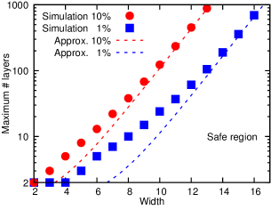
As a practical guide, we constructed a diagram shown in Fig. 3 that includes both theoretical predictions and our numerical tests. We see that as the number of layers increases, the numerical tests match closer to the theoretical results. It is clear from the diagram that a 10-layer NN of width 10 has a probability of dying less than 1% whereas a 10-layer NN of width 5 has a probability of dying greater than 10%; for width of three the probability is about 60%. Note that the growth rate of the maximum number of layers is exponential which is expected by Corollary 3.9.
Refer to caption
Figure 3: Diagram indicating safe operating regions for a ReLU NN. The dash lines represent Corollary 3.9 while the symbols represent our numerical tests. The maximum number of layers of a neural network can be used at different width to keep the probability of collapse less than 1% or 10%. The region below the blue line is the safe region when we design a neural network. As the width increases the theoretical predictions match closer with our numerical simulations.

Our results explain why deep and narrow networks have not been popularly employed in practice and reveal a limitation of training extremely deep networks. We remark that modern practical networks happen to be sufficiently wide enough to have small BDPs. We believe that the born dead network problem is a major impediment for one to explore a potential use of deep and narrow networks.

4 Randomized asymmetric initialization

The so-called ‘He initialization’ [20] is perhaps one of the most popular initialization schemes in deep learning community, especially when the ReLU activation function is concerned. The effectiveness of the He initialization has been shown in many machine learning applications. The He initialization uses mean zero normal distributions. Thus, as we discussed earlier, it suffers from the dying ReLU. We thus propose a new initialization procedure, namely, a randomized asymmetric initialization. The motivation is in twofolds. One is to mimics the He initialization so that the new scheme can produce similar generalization performance. The other is to alleviate the problem of dying ReLU neural networks. We hope that the proposed initialization opens a new way to explore the potential use of deep and narrow networks in practice.

For ease of discussion, we introduce some notation. For any vector 𝒗n+1𝒗superscript𝑛1\bm{v}\in\mathbb{R}^{n+1} and k{1,,n+1}𝑘1𝑛1k\in\{1,\cdots,n+1\}, we define

𝒗k=(v1,,vk1,vk+1,,vn+1)Tn.subscript𝒗𝑘superscriptsubscript𝑣1subscript𝑣𝑘1subscript𝑣𝑘1subscript𝑣𝑛1𝑇superscript𝑛\bm{v}_{-k}=\left(v_{1},\cdots,v_{k-1},v_{k+1},\cdots,v_{n+1}\right)^{T}\in\mathbb{R}^{n}. (6)

In order to train a L𝐿L-layer neural network, we need to initialize 𝜽L={𝑾,𝒃}1Lsubscript𝜽𝐿subscriptsuperscript𝑾superscript𝒃1𝐿\bm{\theta}_{L}=\{\bm{W}^{\ell},\bm{b}^{\ell}\}_{1\leq\ell\leq L}. At each layer, let V=[𝑾,𝒃]N×(N1+1)superscriptVsuperscript𝑾superscript𝒃superscriptsubscript𝑁subscript𝑁11\textbf{V}^{\ell}=[\bm{W}^{\ell},\bm{b}^{\ell}]\in\mathbb{R}^{N_{\ell}\times(N_{\ell-1}+1)}. We denote the j𝑗j-th row of VsuperscriptV\textbf{V}^{\ell} by Vj=[𝑾j,𝒃j]N1+1subscriptsuperscriptV𝑗subscriptsuperscript𝑾𝑗subscriptsuperscript𝒃𝑗superscriptsubscript𝑁11\textbf{V}^{\ell}_{j}=[\bm{W}^{\ell}_{j},\bm{b}^{\ell}_{j}]\in\mathbb{R}^{N_{\ell-1}+1}, j=1,,N𝑗1subscript𝑁j=1,\cdots,N_{\ell} where N0=dinsubscript𝑁0subscript𝑑inN_{0}=d_{\text{in}} and NL=doutsubscript𝑁𝐿subscript𝑑outN_{L}=d_{\text{out}}.

4.1 Proposed initialization

We propose to initialize VsuperscriptV\textbf{V}^{\ell} as follows. Let PsubscriptP\text{P}_{\ell} be a probability distribution defined on [0,M]0subscript𝑀[0,M_{\ell}] for some M>0subscript𝑀0M_{\ell}>0 or [0,)0[0,\infty). Note that PsubscriptP\text{P}_{\ell} is asymmetric around 0. At the first layer of =11\ell=1, we employ the ‘He initialization’ [20], i.e., Wij1N(0,2/din)similar-tosubscriptsuperscriptW1𝑖𝑗𝑁02subscript𝑑in\textbf{W}^{1}_{ij}\sim N(0,2/d_{\text{in}}) and b1=0superscriptb10\textbf{b}^{1}=\textbf{0}. For 22\ell\geq 2, and each 1jN1𝑗subscript𝑁1\leq j\leq N_{\ell}, we initialize 𝑽jsuperscriptsubscript𝑽𝑗\bm{V}_{j}^{\ell} as follows:

  1. 1.

    Randomly choose kjsubscriptsuperscript𝑘𝑗k^{\ell}_{j} in {1,2,,N1,N1+1}12subscript𝑁1subscript𝑁11\{1,2,\cdots,N_{\ell-1},N_{\ell-1}+1\}.

  2. 2.

    Initialize (Vj)kj𝒩(0,σ2𝑰)similar-tosubscriptsubscriptsuperscriptV𝑗subscriptsuperscript𝑘𝑗𝒩0superscriptsubscript𝜎2𝑰(\textbf{V}^{\ell}_{j})_{-k^{\ell}_{j}}\sim\mathcal{N}(0,\sigma_{\ell}^{2}\bm{I}) and (Vj)kjPsimilar-tosubscriptsubscriptsuperscriptV𝑗subscriptsuperscript𝑘𝑗subscriptP(\textbf{V}^{\ell}_{j})_{k^{\ell}_{j}}\sim\text{P}_{\ell}.

Since an index is randomly chosen at each \ell and j𝑗j and a positive number is randomly drawn from an asymmetric probability distribution around 0, we name this new initialization a randomized asymmetric initialization. Only for the first layer, the He initialization is employed. This is because since an input could have a negative value, if the weight which corresponds to the negative input were to be initialized from PsubscriptP\text{P}_{\ell}, this could cause the dying ReLU. We note that the new initialization requires us to choose σ2superscriptsubscript𝜎2\sigma_{\ell}^{2} and PsubscriptP\text{P}_{\ell}. In Subsection 4.2, these will be theoretically determined. One could choose multiple indices in the step 1 of the new initialization. However, for simplicity, we constraint ourselves to a single index case.

We first show that this new initialization procedure results in a smaller upper bound of the BDP.

Theorem 4.1.

For 𝐍L=(din,N1,,NL1,dout)L+1subscript𝐍𝐿subscript𝑑insubscript𝑁1subscript𝑁𝐿1subscript𝑑outsuperscript𝐿1\vec{\bm{N}}_{L}=(d_{\text{in}},N_{1},\cdots,N_{L-1},d_{\text{out}})\in\mathbb{N}^{L+1}, let 𝛉𝐍L={𝐖,𝐛}1Lsubscript𝛉subscript𝐍𝐿subscriptsuperscript𝐖superscript𝐛1𝐿\bm{\theta}_{\vec{\bm{N}}_{L}}=\{\bm{W}^{\ell},\bm{b}^{\ell}\}_{1\leq\ell\leq L} and 𝒩L(x;𝛉𝐍L)superscript𝒩𝐿xsubscript𝛉subscript𝐍𝐿\mathcal{N}^{L}(\textbf{x};\bm{\theta}_{\vec{\bm{N}}_{L}}) be a ReLU neural network with L𝐿L layers, each having N1,,NL1subscript𝑁1subscript𝑁𝐿1N_{1},\cdots,N_{L-1} neurons. Suppose 𝛉𝐍Lsubscript𝛉subscript𝐍𝐿\bm{\theta}_{\vec{\bm{N}}_{L}} is initialized by the randomized asymmetric initialization (RAI). Then,

P(𝔍𝑵L)1=1L1(1(1/2γ)N),𝑃subscript𝔍subscript𝑵𝐿1superscriptsubscriptproduct1𝐿11superscript12subscript𝛾subscript𝑁P(\mathfrak{J}_{\vec{\bm{N}}_{L}})\leq 1-\prod_{\ell=1}^{L-1}\left(1-\left(1/2-\gamma_{\ell}\right)^{N_{\ell}}\right),

where 𝔍𝐍Lsubscript𝔍subscript𝐍𝐿\mathfrak{J}_{\vec{\bm{N}}_{L}} is defined in (3), γ1=0subscript𝛾10\gamma_{1}=0 and γjsubscript𝛾𝑗\gamma_{j}’s are some constants in (0,0.5]00.5(0,0.5], which depend on {N}=1L1superscriptsubscriptsubscript𝑁1𝐿1\{N_{\ell}\}_{\ell=1}^{L-1} and the training input data 𝒟𝒟\mathcal{D}.

Proof 4.2.

The proof can be found in Appendix E.

When a symmetric initialization is employed, γj=0subscript𝛾𝑗0\gamma_{j}=0 for all 1j<NL1𝑗subscript𝑁𝐿1\leq j<N_{L}, which results in Equation 5 of Theorem 3.3. Although the new initialization has a smaller upper bound compared to those by symmetric initialization, as Theorem 3.1 suggests, it also asymptotically suffers from the dying ReLU.

Corollary 4.3.

Assuming the same conditions in Theorem 4.1, and N=Nsubscript𝑁𝑁N_{\ell}=N for all \ell. Let 𝔍𝐍Lsubscript𝔍subscript𝐍𝐿\mathfrak{J}_{\vec{\bm{N}}_{L}} be the event defined in (3). Then, there exists 2<γ2𝛾2<\gamma, which depends on N,L𝑁𝐿N,L and the training input data 𝒟𝒟\mathcal{D}, such that

P(𝔍𝑵L)1=1L1(1(1/γ)N).𝑃subscript𝔍subscript𝑵𝐿1superscriptsubscriptproduct1𝐿11superscript1𝛾𝑁P(\mathfrak{J}_{\vec{\bm{N}}_{L}})\leq 1-\prod_{\ell=1}^{L-1}\left(1-(1/\gamma)^{N}\right).

For fixed depth L𝐿L and δ>0𝛿0\delta>0, if the width N𝑁N is N=logγL/δ𝑁subscript𝛾𝐿𝛿N=\log_{\gamma}L/\delta, we have P(𝔍𝐍Lc)>1δ𝑃superscriptsubscript𝔍subscript𝐍𝐿𝑐1𝛿P(\mathfrak{J}_{\vec{\bm{N}}_{L}}^{c})>1-\delta, where 𝔍𝐍Lcsuperscriptsubscript𝔍subscript𝐍𝐿𝑐\mathfrak{J}_{\vec{\bm{N}}_{L}}^{c} is the complement of 𝔍𝐍Lsubscript𝔍subscript𝐍𝐿\mathfrak{J}_{\vec{\bm{N}}_{L}}. Furthermore,

limLP(𝔍𝑵L)=1,limNP(𝔍𝑵L)=0.\begin{split}\lim_{L\to\infty}P(\mathfrak{J}_{\vec{\bm{N}}_{L}})=1,\qquad\lim_{N\to\infty}P(\mathfrak{J}_{\vec{\bm{N}}_{L}})=0.\end{split}
Proof 4.4.

The proof is readily followed from Theorem 3.14.1 and Corollary 3.9.

4.2 Second moment analysis

The proposed randomized asymmetric initialization (RAI) described in Subsection 4.1 requires us to determine σ2superscriptsubscript𝜎2\sigma_{\ell}^{2} and PsubscriptP\text{P}_{\ell}. Similar to the He initialization ([21]), we aim to properly choose initialization parameters from the length map analysis. Following the work of [39], we present the analysis of a single input propagation through the deep ReLU network. To be more precise, for a network architecture 𝑵=(din,N1,,N1,N)+1subscript𝑵subscript𝑑insubscript𝑁1subscript𝑁1subscript𝑁superscript1\vec{\bm{N}}_{\ell}=(d_{\text{in}},N_{1},\cdots,N_{\ell-1},N_{\ell})\in\mathbb{N}^{\ell+1}, we track the expectation of the normalized squared length of the input vector at each layer, 𝔼[q(x;𝜽𝑵)]𝔼delimited-[]superscript𝑞xsubscript𝜽subscript𝑵\mathbb{E}[q^{\ell}(\textbf{x};\bm{\theta}_{\vec{\bm{N}}_{\ell}})], where q(x;𝜽𝑵)=𝒩(x;𝜽𝑵)2Nsuperscript𝑞xsubscript𝜽subscript𝑵superscriptnormsuperscript𝒩xsubscript𝜽subscript𝑵2subscript𝑁q^{\ell}(\textbf{x};\bm{\theta}_{\vec{\bm{N}}_{\ell}})=\frac{\|\mathcal{N}^{\ell}(\textbf{x};\bm{\theta}_{\vec{\bm{N}}_{\ell}})\|^{2}}{N_{\ell}}. The expectation 𝔼𝔼\mathbb{E} is taken with respect to all weights and biases 𝜽𝑵subscript𝜽subscript𝑵\bm{\theta}_{\vec{\bm{N}}_{\ell}}.

Theorem 4.5.

For 𝐍=(din,N1,,N1,N)+1subscript𝐍subscript𝑑insubscript𝑁1subscript𝑁1subscript𝑁superscript1\vec{\bm{N}}_{\ell}=(d_{\text{in}},N_{1},\cdots,N_{\ell-1},N_{\ell})\in\mathbb{N}^{\ell+1}, let 𝛉𝐍={𝐖j,𝐛j}1jsubscript𝛉subscript𝐍subscriptsuperscript𝐖𝑗superscript𝐛𝑗1𝑗\bm{\theta}_{\vec{\bm{N}}_{\ell}}=\{\bm{W}^{j},\bm{b}^{j}\}_{1\leq j\leq\ell} be initialized by the RAI with the following σ2superscriptsubscript𝜎2\sigma_{\ell}^{2} and PsubscriptP\text{P}_{\ell}. Let σ2:=σw2N1assignsuperscriptsubscript𝜎2superscriptsubscript𝜎𝑤2subscript𝑁1\sigma_{\ell}^{2}:=\frac{\sigma_{w}^{2}}{N_{\ell-1}} for some σw2superscriptsubscript𝜎𝑤2\sigma_{w}^{2} and let PsubscriptP\text{P}_{\ell} be a probability distribution whose support is [0,M]+0subscript𝑀superscript[0,M_{\ell}]\subset\mathbb{R}^{+} such that μ,i=E[Xi]<superscriptsubscript𝜇𝑖𝐸delimited-[]superscriptsubscript𝑋𝑖\mu_{\ell,i}^{\prime}=E[X_{\ell}^{i}]<\infty, for i=1,2𝑖12i=1,2, where XPsimilar-tosubscript𝑋subscriptPX_{\ell}\sim\text{P}_{\ell} and μ,1M/2superscriptsubscript𝜇1subscript𝑀2\mu_{\ell,1}^{\prime}\geq M_{\ell}/2. Then for any input xdinxsuperscriptsubscript𝑑𝑖𝑛\textbf{x}\in\mathbb{R}^{d_{in}}, we have

𝒜low,2𝔼[q(x;𝜽𝑵)]+σb,2𝔼[q+1(x;𝜽𝑵+1)]𝒜upp,2𝔼[q(x;𝜽𝑵)]+σb,2,subscript𝒜𝑙𝑜𝑤2𝔼delimited-[]superscript𝑞xsubscript𝜽subscript𝑵superscriptsubscript𝜎𝑏2𝔼delimited-[]superscript𝑞1xsubscript𝜽subscript𝑵1subscript𝒜𝑢𝑝𝑝2𝔼delimited-[]superscript𝑞xsubscript𝜽subscript𝑵superscriptsubscript𝜎𝑏2\displaystyle\frac{\mathcal{A}_{low,\ell}}{2}\mathbb{E}[q^{\ell}(\textbf{x};\bm{\theta}_{\vec{\bm{N}}_{\ell}})]+\sigma_{b,\ell}^{2}\leq\mathbb{E}[q^{\ell+1}(\textbf{x};\bm{\theta}_{\vec{\bm{N}}_{\ell+1}})]\leq\frac{\mathcal{A}_{upp,\ell}}{2}\mathbb{E}[q^{\ell}(\textbf{x};\bm{\theta}_{\vec{\bm{N}}_{\ell}})]+\sigma_{b,\ell}^{2},

where σb,2=μ+1,2+σ+12N+1N+1+1superscriptsubscript𝜎𝑏2superscriptsubscript𝜇12superscriptsubscript𝜎12subscript𝑁1subscript𝑁11\sigma_{b,\ell}^{2}=\frac{\mu_{\ell+1,2}^{\prime}+\sigma_{\ell+1}^{2}N_{\ell+1}}{N_{\ell+1}+1}, 𝒜low,=σb,+12σb,2(Nμ,2+N1σw2N1+1)subscript𝒜𝑙𝑜𝑤superscriptsubscript𝜎𝑏12superscriptsubscript𝜎𝑏2subscript𝑁superscriptsubscript𝜇2subscript𝑁1superscriptsubscript𝜎𝑤2subscript𝑁11\mathcal{A}_{low,\ell}=\frac{\sigma_{b,\ell+1}^{2}}{\sigma_{b,\ell}^{2}}\left(\frac{N_{\ell}\mu_{\ell,2}^{\prime}+N_{\ell-1}\sigma_{w}^{2}}{N_{\ell-1}+1}\right), and

𝒜upp,=σb,+12σb,2(N1σw2+22/πNμ,1σw+2Nμ,2N1+1).subscript𝒜𝑢𝑝𝑝superscriptsubscript𝜎𝑏12superscriptsubscript𝜎𝑏2subscript𝑁1superscriptsubscript𝜎𝑤222𝜋subscript𝑁superscriptsubscript𝜇1subscript𝜎𝑤2subscript𝑁superscriptsubscript𝜇2subscript𝑁11\mathcal{A}_{upp,\ell}=\frac{\sigma_{b,\ell+1}^{2}}{\sigma_{b,\ell}^{2}}\left(\frac{N_{\ell-1}\sigma_{w}^{2}+2\sqrt{2/\pi}N_{\ell}\mu_{\ell,1}^{\prime}\sigma_{w}+2N_{\ell}\mu_{\ell,2}^{\prime}}{N_{\ell-1}+1}\right).
Proof 4.6.

The proof can be found in Appendix F.

Corollary 4.7.

Under the same conditions of Theorem 4.5, if N=Nsubscript𝑁𝑁N_{\ell}=N, M=Msubscript𝑀𝑀M_{\ell}=M, E[Xi]=μi𝐸delimited-[]superscriptsubscript𝑋𝑖superscriptsubscript𝜇𝑖E[X_{\ell}^{i}]=\mu_{i}^{\prime}, i=1,2𝑖12i=1,2 for all \ell, and μ1M/2superscriptsubscript𝜇1𝑀2\mu_{1}^{\prime}\geq M/2, we have

𝒜low,2𝔼[q(x;𝜽𝑵)]+σb,2𝔼[q+1(x;𝜽𝑵+1)]𝒜upp,2𝔼[q(x;𝜽𝑵)]+σb,2,subscript𝒜𝑙𝑜𝑤2𝔼delimited-[]superscript𝑞xsubscript𝜽subscript𝑵superscriptsubscript𝜎𝑏2𝔼delimited-[]superscript𝑞1xsubscript𝜽subscript𝑵1subscript𝒜𝑢𝑝𝑝2𝔼delimited-[]superscript𝑞xsubscript𝜽subscript𝑵superscriptsubscript𝜎𝑏2\displaystyle\frac{\mathcal{A}_{low,\ell}}{2}\mathbb{E}[q^{\ell}(\textbf{x};\bm{\theta}_{\vec{\bm{N}}_{\ell}})]+\sigma_{b,\ell}^{2}\leq\mathbb{E}[q^{\ell+1}(\textbf{x};\bm{\theta}_{\vec{\bm{N}}_{\ell+1}})]\leq\frac{\mathcal{A}_{upp,\ell}}{2}\mathbb{E}[q^{\ell}(\textbf{x};\bm{\theta}_{\vec{\bm{N}}_{\ell}})]+\sigma_{b,\ell}^{2},

where σb,2=μ2+σw2N+1superscriptsubscript𝜎𝑏2superscriptsubscript𝜇2superscriptsubscript𝜎𝑤2𝑁1\sigma_{b,\ell}^{2}=\frac{\mu_{2}^{\prime}+\sigma_{w}^{2}}{N+1}, 𝒜low,=N(μ2+σw2)N+1subscript𝒜𝑙𝑜𝑤𝑁superscriptsubscript𝜇2superscriptsubscript𝜎𝑤2𝑁1\mathcal{A}_{low,\ell}=\frac{N(\mu_{2}^{\prime}+\sigma_{w}^{2})}{N+1}, and 𝒜upp,=N(σw2+22/πμ1σw+2μ2)N+1subscript𝒜𝑢𝑝𝑝𝑁superscriptsubscript𝜎𝑤222𝜋superscriptsubscript𝜇1subscript𝜎𝑤2superscriptsubscript𝜇2𝑁1\mathcal{A}_{upp,\ell}=\frac{N(\sigma_{w}^{2}+2\sqrt{2/\pi}\mu_{1}^{\prime}\sigma_{w}+2\mu_{2}^{\prime})}{N+1}.

Since σb,2>0superscriptsubscript𝜎𝑏20\sigma_{b,\ell}^{2}>0, lim𝔼[q(x;𝜽𝑵)]subscript𝔼delimited-[]superscript𝑞xsubscript𝜽subscript𝑵\lim_{\ell\to\infty}\mathbb{E}[q^{\ell}(\textbf{x};\bm{\theta}_{\vec{\bm{N}}_{\ell}})] cannot be zero. In order for lim𝔼[q(x;𝜽𝑵)]<subscript𝔼delimited-[]superscript𝑞xsubscript𝜽subscript𝑵\lim_{\ell\to\infty}\mathbb{E}[q^{\ell}(\textbf{x};\bm{\theta}_{\vec{\bm{N}}_{\ell}})]<\infty, the initialization parameters (σw2,μ,1,μ,2)superscriptsubscript𝜎𝑤2superscriptsubscript𝜇1superscriptsubscript𝜇2(\sigma_{w}^{2},\mu_{\ell,1}^{\prime},\mu_{\ell,2}^{\prime}) have to be chosen to satisfy 𝒜upp,<2subscript𝒜𝑢𝑝𝑝2\mathcal{A}_{upp,\ell}<2. Assuming μ2<1superscriptsubscript𝜇21\mu_{2}^{\prime}<1, if σwsubscript𝜎𝑤\sigma_{w} is chosen to be

σw=2(μ1π+μ12π+1μ2),subscript𝜎𝑤2superscriptsubscript𝜇1𝜋superscriptsubscript𝜇12𝜋1superscriptsubscript𝜇2\sigma_{w}=\sqrt{2}\left(-\frac{\mu_{1}^{\prime}}{\sqrt{\pi}}+\sqrt{\frac{\mu_{1}^{\prime 2}}{\pi}+1-\mu_{2}^{\prime}}\right), (7)

we have 𝒜upp,2=NN+1subscript𝒜𝑢𝑝𝑝2𝑁𝑁1\frac{\mathcal{A}_{upp,\ell}}{2}=\frac{N}{N+1} which satisfies the condition.

Refer to caption
Refer to caption
Refer to caption
Refer to caption
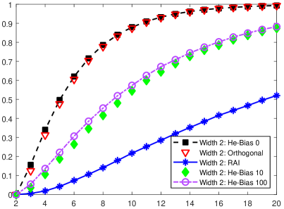
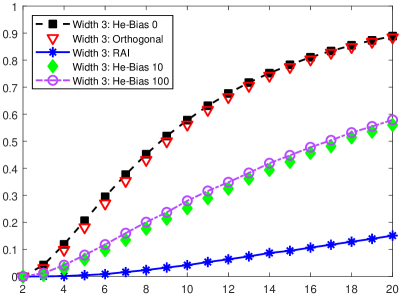
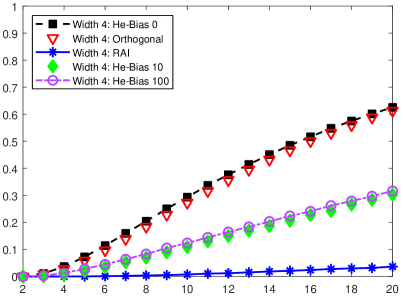
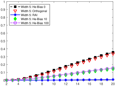
Figure 4: The BDPs are plotted with respect to increasing the number of depth L𝐿L at varying width N=2𝑁2N=2 (top left), N=3𝑁3N=3 (top right), N=4𝑁4N=4 (bottom left) and N=5𝑁5N=5 (bottom right). The ReLU neural networks in din=1subscript𝑑in1d_{\text{in}}=1 are employed. The square, diamond and circle symbols correspond to the He initialization [20] with constant bias 0, 10 and 100, respectively. The inverted triangle symbols correspond to the orthogonal initialization [43]. The asterisk symbols correspond to the proposed randomized asymmetric initialization (RAI).
Refer to caption
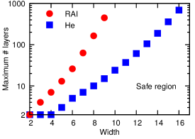
Figure 5: Comparison of the safe operating regions for a ReLU NN between RAI and He initializations. The maximum number of layers of a neural network can be used at different width to keep the probability of collapse less than 1%.

4.3 Comparison against other initialization procedures

In Fig. 4, we demonstrate the probability that the network is BD by the proposed randomized asymmetric initialization (RAI) method. Here we employ P=Beta(2,1)PBeta21\text{P}=\text{Beta}(2,1) and σw=223π+1+89π0.6007subscript𝜎𝑤223𝜋189𝜋0.6007\sigma_{w}=-\frac{2\sqrt{2}}{3\sqrt{\pi}}+\sqrt{1+\frac{8}{9\pi}}\approx 0.6007 from Equation 7 (see Appendix G for the Python code). To compare against other procedures, we present the results by the He initialization [20]. We also present the results of existing asymmetric initialization procedures; the orthogonal [43] and the layer-sequential unit-variance (LSUV) [34] initializations. The LSUV is the orthogonal initialization combined with rescaling of weights such that the output of each layer has unit variance. Because weight rescaling cannot make the output escape from the negative part of ReLU, it is sufficient to consider the orthogonal initialization. We see that the BDPs by the orthogonal initialization are very close to and a little lower than those by the He initialization. This implies that the orthogonal initialization cannot prevent the dying ReLU network. Furthermore, we show the results by the He initialization with positive constant bias of 10 and 100. Naively speaking, having a big positive bias will help in preventing dying ReLU neurons, as the input of each layer is pushed to be positive, although this might cause the exploding gradient problem in training. We see that the BDPs by the He with bias 10 and 100 are lower than those by the He with bias 0 and the orthogonal initialization. However, it is clearly observed that our proposed initialization (RAI) drastically drops the BDPs compared to all others. This is implied by Theorem 4.1.

As a practical guide, we constructed a diagram shown in Fig. 5 to demonstrate the 1% safe operation region by the RAI. It is clear from the diagram that the RAI drastically expands its 1% safe region compared to those by the He initialization. Note that the growth rate of the maximum number of layers is exponential which is expected by Corollary 4.3.

5 Numerical examples

We demonstrate the effectiveness of the proposed randomized asymmetric initialization (RAI) in training deep ReLU networks.

Test functions include one- and two-dimensional functions of different regularities. The following test functions are employed as unknown target functions. For one dimensional cases,

f1(x)=|x|,f2(x)=xsin(5x),f3(x)=1{x>0}(x)+0.2sin(5x).\begin{split}f_{1}(x)=|x|,\qquad f_{2}(x)=x\sin(5x),\qquad f_{3}(x)=1_{\{x>0\}}(x)+0.2\sin(5x).\end{split} (8)

For two dimensional case,

f4(x1,x2)=[|x1+x2||x1x2|].subscript𝑓4subscript𝑥1subscript𝑥2matrixsubscript𝑥1subscript𝑥2subscript𝑥1subscript𝑥2f_{4}(x_{1},x_{2})=\begin{bmatrix}|{x}_{1}+{x}_{2}|\\ |{x}_{1}-{x}_{2}|\end{bmatrix}. (9)

We employ the network architecture having the width of din+doutsubscript𝑑insubscript𝑑outd_{\text{in}}+d_{\text{out}} at all layers. Here dinsubscript𝑑ind_{\text{in}} and doutsubscript𝑑outd_{\text{out}} are the dimensions of the input and output, respectively. It was shown in [18] that the minimum number of width required for the universal approximation is less than or equal to din+doutsubscript𝑑insubscript𝑑outd_{\text{in}}+d_{\text{out}}. We thus choose this specific network architecture. as it theoretically guarantees to approximate any continuous function. In all numerical examples, we employ one of the most popular first-order gradient-based optimization, Adam [27] with the default parameters. The minibatch size is chosen to be either 64 or 128. The standard L2subscript𝐿2L_{2}-loss function (𝒩L(x,𝜽),(x,y))=(𝒩L(x;𝜽)y)2superscript𝒩𝐿x𝜽x𝑦superscriptsuperscript𝒩𝐿x𝜽𝑦2\ell(\mathcal{N}^{L}(\textbf{x},\bm{\theta}),(\textbf{x},y))=(\mathcal{N}^{L}(\textbf{x};\bm{\theta})-y)^{2} is used on 3,000 training data. The training data are randomly uniformly drawn from [3,3]dinsuperscript33subscript𝑑in[-\sqrt{3},\sqrt{3}]^{d_{\text{in}}}. Without changing any setups described above, we present the approximation results based on different initialization procedures. The results by our proposed randomized asymmetric initialization are referred to ‘Rand. Asymmetric’ or ‘RAI’. Specifically, we use P=Beta(2,1)PBeta21\text{P}=\text{Beta}(2,1) with σwsubscript𝜎𝑤\sigma_{w} defined in Equation 7. To compare against other methods, we also show the results by the He initialization [20]. We present the ensemble of 1,000 independent training simulations.

In one dimensional examples, we employ a 10-layer ReLU network of width 2. It follows from Fig. 4 that we expect to observe at least 88% training results by the symmetric initialization and 22% training results by the RAI are collapsed. In the two dimensional example, we employ a 20-layer ReLU network of width 4. According to Fig. 4, we expect to see at least 63% training results by the symmetric initialization and 3.7% training results by the RAI are collapsed.

Fig. 6 shows all training outcomes of our 1,000 simulations for approximating f1(x)subscript𝑓1𝑥f_{1}(x) and its corresponding empirical probabilities by different initialization schemes. For this specific test function, we observe only 3 trained results shown in A, B, C. In fact, f1(x)subscript𝑓1𝑥f_{1}(x) can be represented exactly by a 2-layer ReLU network with width 2, f1(x)=|x|=ReLU(x)+ReLU(x)subscript𝑓1𝑥𝑥ReLU𝑥ReLU𝑥f_{1}(x)=|x|=\text{ReLU}(x)+\text{ReLU}(-x). It can clearly be seen that the He initialization results in the collapse with probability more than 90%. However, this probability is drastically reduced to 40% by the RAI. These probabilities are different from the probability that the network is BD. This implies that even though the network wasn’t BD, there are cases that after training, the network dies. In this example, 5.6% and 18.3% of results by the symmetric and our method, respectively, are not dead at the initialization, however, they are ended up with collapsing after training. The 37.3% of training results by the RAI perfectly recover the target function f1(x)subscript𝑓1𝑥f_{1}(x), however, only 2.2% of results by the He initialization achieve this success. Also, 22.4% of the RAI and 4.2% of the He initialization produce the half-trained results which correspond to Fig. 6 (B). We remark that the only difference in training is the initialization. This implies that our new initialization does not only prevent the dying ReLU network but also improves the quality of the training in this case.

Refer to caption
𝒇𝟏(𝒙)subscript𝒇1𝒙\small\bm{f_{1}(x)} Collapse (A) Half-Trained (B) Success (C)
Symmetric (He init.) 93.6% 4.2% 2.2%
Rand. Asymmetric 40.3% 22.4% 37.3%
Figure 6: The approximation results for f1(x)subscript𝑓1𝑥f_{1}(x) using a 10-layer ReLU network of width 2. For this specific test function, we observe only 3 trained results shown in A, B, C. The table shows the corresponding empirical probabilities from 1,000 independent simulations. The only difference is the initialization.

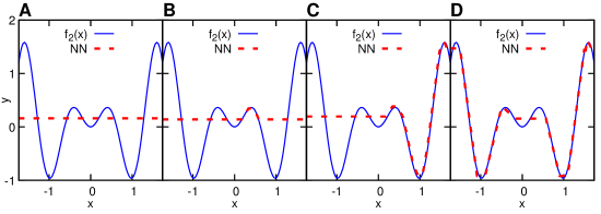
The approximation results for f2(x)subscript𝑓2𝑥f_{2}(x) are shown in Fig. 7. Note that f2subscript𝑓2f_{2} is a Csuperscript𝐶C^{\infty} function. It can be seen that 91.9% of training results by the symmetric initialization and 29.2% of training results by the RAI are collapsed which correspond to Fig. 7 (A). This indicates that the RAI can effectively alleviate the dying ReLU. In this example, 3.9% and 7.2% of results by the symmetric and our method, respectively, are not dead at the initialization, however, they are ended up with collapsing after training. Except for the collapse, other training outcomes are not easy to be classified. Fig. 7 (B,C,D) shows three training results among many others. We observe that the behavior and result of training are not easily predictable in general. However, we consistently observe partially collapsed results after training. Such partial collapses are also observed in Fig. 7 (B,C,D). We believe that this requires more attention and postpone the study of this partial collapse to future work.
Refer to caption
𝒇𝟐(𝒙)subscript𝒇2𝒙\small\bm{f_{2}(x)} Collapsed (A) Not collapsed (B,C,D)
Symmetric (He init.) 91.9% 8.1%
Rand. Asymmetric 29.2% 70.8%
Figure 7: The approximation results for f2(x)subscript𝑓2𝑥f_{2}(x) using a 10-layer ReLU network of width 2. Among many trained results, four are shown. The table shows the corresponding empirical probabilities from 1,000 independent simulations. The only difference is the initialization.
Refer to caption
𝒇𝟑(𝒙)subscript𝒇3𝒙\small\bm{f_{3}(x)} Collapsed (A) Not collapsed (B,C,D)
Symmetric (He init.) 93.8% 6.2%
Rand. Asymmetric 32.6% 67.4%
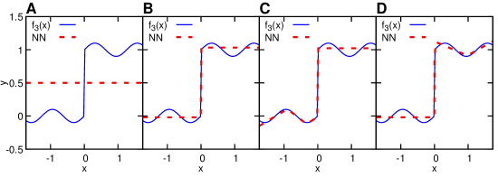
Figure 8: The approximation results for f3(x)subscript𝑓3𝑥f_{3}(x) using a 10-layer ReLU network of width 2. Among many trained results, four are shown. The table shows the corresponding empirical probabilities from 1,000 independent simulations. The only difference is the initialization.

Similar behavior is observed for approximating a discontinuous function f3(x)subscript𝑓3𝑥f_{3}(x). The approximation results for f3(x)subscript𝑓3𝑥f_{3}(x) and its corresponding empirical probabilities are shown in Fig. 8. We see that 93.8% of training results by the He initialization and 32.6% of training results by the RAI are collapsed which correspond to Fig. 8 (A). In this example, the RAI drops the probability of collapsing by 60.3 percentage point. Again, this implies that the RAI can effectively avoid the dying ReLU, especially when deep and narrow ReLU networks are employed. Fig. 8 (B,C,D) shows three trained results among many others. Again, we observe partially collapsed results.

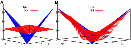
Next we show the approximation result for a multi-dimensional inputs and outputs function f4(x)subscript𝑓4xf_{4}(\textbf{x}) defined in Equation 9. We observe similar behavior. Fig. 9 shows some of approximation results for f4subscript𝑓4f_{4} and its corresponding probabilities. Among 1,000 independent simulations, the collapsed results are obtained by the He initialization with 76.8% probability and by the RAI with 9.6% probability. From Fig. 4, we expect to observe at least 63% and 3.7% of results by the symmetric and the RAI to be collapsed. Thus, in this example, 13.8% and 5.9% of results by the symmetric and our method, respectively, are not dead at the initialization, however, they are ended up with Fig. 9 (A) after training. This indicates that the RAI can also effectively overcome the dying ReLU in multi-dimensional inputs and outputs tasks.
Refer to caption
𝒇𝟒(𝒙)subscript𝒇4𝒙\small\bm{f_{4}(x)} Collapsed (A) Not collapsed (B)
Symmetric (He init.) 76.8% 23.2%
Rand. Asymmetric 9.6% 90.4%
Figure 9: The approximation results for f4(x)subscript𝑓4xf_{4}(\textbf{x}) using a 20-layer ReLU network of width 4. Among many trained results, two are shown. The table shows the corresponding empirical probabilities from 1,000 independent simulations. The only difference is the initialization.

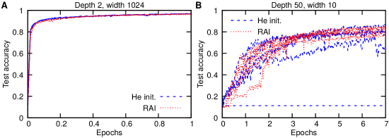
As a last example, we demonstrate the performance of the RAI on the MNIST dataset. For the training, we employ the cross-entropy loss and the mini-batch size of 100. The networks are trained using Adam [27] with its default values. In Fig. 10, the convergence of the test accuracy is shown with respect to the number of epochs. On the left and right, we employ the ReLU network of depth 2 and width 1024 and of depth 50 and with 10, respectively. We see that when the shallow and wide network is employed, the RAI and the He initialization show similar generalization performance (test accuracy). However, when the deep and narrow network is employed, the RAI performs better than the He initialization. This indicates that the proposed RAI not only reduces the BDP of deep networks, but also has good generalization performance.
Refer to caption
Figure 10: The test accuracy on the MNIST of five independent simulations are shown with respect to the number of epochs by the He initialization and the RAI. (Left) A shallow (depth 2, width 1024) ReLU network is employed. The He initialization and the RAI have similar performance. (Right) A deep (depth 50, width 10) ReLU network is employed. The RAI results in higher test accuracy than the He initialization.

6 Conclusion

In this paper, we establish, to the best of our knowledge, the first theoretical analysis on the dying ReLU. By focusing on the worst case of dying ReLU, we define ‘the dying ReLU network’ which refers to the problem when the ReLU network is dead. We categorize the dying process into two phases. One phase is the event where the ReLU network is initialized to be a constant function. We refer to this event as ‘the network is born dead’. The other phase is the event where the ReLU network is collapsed after training. Certainly, the first phase implies the second, but not vice versa. We show that the probability that the network is born dead goes to 1 as the depth goes infinite. Also, we provide an upper and a lower bound of the dying probability in din=1subscript𝑑in1d_{\text{in}}=1 when the standard symmetric initialization is used.

Furthermore, in order to overcome the dying ReLU networks, we propose a new initialization procedure, namely, a randomized asymmetric initialization (RAI). We show that the RAI has a smaller upper bound of the probability of NNs being born dead. By establishing the expected length map relation (second moment analysis), all parameters needed for the new method are theoretically designed. Numerical examples are provided to demonstrate the performance of our method. We observe that the RAI does not only overcome the dying ReLU but also improves the training and generalization performance.

Acknowledgements

This work received support by the DARPA EQUiPS grant N66001-15-2-4055, the AFOSR grant FA9550-17-1-0013, and the DARPA AIRA grant HR00111990025. The research of the third author was partially supported by the NSF of China 11771083 and the NSF of Fujian 2017J01556, 2016J01013.

Appendix A Proof of Theorem 3.1

The proof starts with the following lemma.

Lemma A.1.

Let 𝒩L(x)superscript𝒩𝐿x\mathcal{N}^{L}(\textbf{x}) be a L𝐿L-layer ReLU neural network with Nsubscript𝑁N_{\ell} neurons at the \ell-th layer. Suppose all weights are randomly independently generated from probability distributions satisfying P(𝐖j𝐳=𝟎)=0𝑃superscriptsubscript𝐖𝑗𝐳00P(\bm{W}_{j}^{\ell}\bm{z}=\bm{0})=0 for any nonzero vector 𝐳N1𝐳superscriptsubscript𝑁1\bm{z}\in\mathbb{R}^{N_{\ell-1}} and any j𝑗j-th row of 𝐖superscript𝐖\bm{W}^{\ell}. Then

P(𝔍𝑵L)=P({1,,L1} such that ϕ(𝒩(x))=𝟎x𝒟),𝑃subscript𝔍subscript𝑵𝐿𝑃1𝐿1 such that italic-ϕsuperscript𝒩x0for-allx𝒟P(\mathfrak{J}_{\vec{\bm{N}}_{L}})=P(\exists\hskip 2.84544pt\ell\in\{1,\dots,L-1\}\text{ such that }\phi(\mathcal{N}^{\ell}(\textbf{x}))=\bm{0}\hskip 2.84544pt\forall\textbf{x}\in\mathcal{D}),

where 𝒟Br(𝟎)={xdin|x<r}𝒟subscript𝐵𝑟0conditional-setxsuperscriptsubscript𝑑innorm𝑥𝑟\mathcal{D}\subset B_{r}(\bm{0})=\{\textbf{x}\in\mathbb{R}^{d_{\text{in}}}|\|x\|<r\} for any r>0𝑟0r>0 and 𝔍𝐍Lsubscript𝔍subscript𝐍𝐿\mathfrak{J}_{\vec{\bm{N}}_{L}} is the event defined in (3).

Proof A.2.

Suppose 𝒩L(x)=𝒩L(𝟎)superscript𝒩𝐿xsuperscript𝒩𝐿0\mathcal{N}^{L}(\textbf{x})=\mathcal{N}^{L}(\bm{0}) for all x𝒟Br(𝟎)x𝒟subscript𝐵𝑟0\textbf{x}\in\mathcal{D}\subset B_{r}(\bm{0}). Then ϕ(𝒩L1(x))=ϕ(𝒩L1(𝟎))italic-ϕsuperscript𝒩𝐿1xitalic-ϕsuperscript𝒩𝐿10\phi(\mathcal{N}^{L-1}(\textbf{x}))=\phi(\mathcal{N}^{L-1}(\bm{0})) for all x𝒟x𝒟\textbf{x}\in\mathcal{D}. If ϕ(𝒩L1(x))=ϕ(𝒩L1(𝟎))=𝟎italic-ϕsuperscript𝒩𝐿1xitalic-ϕsuperscript𝒩𝐿100\phi(\mathcal{N}^{L-1}(\textbf{x}))=\phi(\mathcal{N}^{L-1}(\bm{0}))=\bm{0}, we are done as =L1𝐿1\ell=L-1. If it is not the case, there exists j𝑗j in {1,,NL1}1subscript𝑁𝐿1\{1,\cdots,N_{L-1}\} such that for all x𝒟x𝒟\textbf{x}\in\mathcal{D},

(𝒩L1(x))j=𝑾jL1ϕ(𝒩L2(x))+𝒃jL1=𝑾jL1ϕ(𝒩L2(𝟎))+𝒃jL1=(𝒩L1(𝟎))j>0.subscriptsuperscript𝒩𝐿1x𝑗subscriptsuperscript𝑾𝐿1𝑗italic-ϕsuperscript𝒩𝐿2xsubscriptsuperscript𝒃𝐿1𝑗subscriptsuperscript𝑾𝐿1𝑗italic-ϕsuperscript𝒩𝐿20subscriptsuperscript𝒃𝐿1𝑗subscriptsuperscript𝒩𝐿10𝑗0(\mathcal{N}^{L-1}(\textbf{x}))_{j}=\bm{W}^{L-1}_{j}\phi(\mathcal{N}^{L-2}(\textbf{x}))+\bm{b}^{L-1}_{j}=\bm{W}^{L-1}_{j}\phi(\mathcal{N}^{L-2}(\bm{0}))+\bm{b}^{L-1}_{j}=(\mathcal{N}^{L-1}(\bm{0}))_{j}>0.

Thus we have 𝐖jL1(ϕ(𝒩L2(x))ϕ(𝒩L2(𝟎)))=0subscriptsuperscript𝐖𝐿1𝑗italic-ϕsuperscript𝒩𝐿2xitalic-ϕsuperscript𝒩𝐿200\bm{W}^{L-1}_{j}\left(\phi(\mathcal{N}^{L-2}(\textbf{x}))-\phi(\mathcal{N}^{L-2}(\bm{0}))\right)=0 for all x𝒟x𝒟\textbf{x}\in\mathcal{D}. Let consider the following events:

GL1:={𝑾jL1ϕ(𝒩L2(x))=𝑾jL1ϕ(𝒩L2(𝟎)),x𝒟},assignsubscript𝐺𝐿1formulae-sequencesubscriptsuperscript𝑾𝐿1𝑗italic-ϕsuperscript𝒩𝐿2xsubscriptsuperscript𝑾𝐿1𝑗italic-ϕsuperscript𝒩𝐿20for-allx𝒟\displaystyle G_{L-1}:=\{\bm{W}^{L-1}_{j}\phi(\mathcal{N}^{L-2}(\textbf{x}))=\bm{W}^{L-1}_{j}\phi(\mathcal{N}^{L-2}(\bm{0})),\forall\textbf{x}\in\mathcal{D}\},
RL2:={ϕ(𝒩L2(𝒙))=ϕ(𝒩L2(𝟎)),x𝒟}.assignsubscript𝑅𝐿2formulae-sequenceitalic-ϕsuperscript𝒩𝐿2𝒙italic-ϕsuperscript𝒩𝐿20for-allx𝒟\displaystyle R_{L-2}:=\{\phi(\mathcal{N}^{L-2}(\bm{x}))=\phi(\mathcal{N}^{L-2}(\bm{0})),\forall\textbf{x}\in\mathcal{D}\}.

Note that P(GL1|RL2)=1𝑃conditionalsubscript𝐺𝐿1subscript𝑅𝐿21P(G_{L-1}|R_{L-2})=1. Also, since P(𝐖𝐳)=0𝑃superscript𝐖𝐳0P(\bm{W}^{\ell}\bm{z})=0 for any nonzero vector 𝐳𝐳\bm{z}, we have P(GL1|RL2c)=0𝑃conditionalsubscript𝐺𝐿1superscriptsubscript𝑅𝐿2𝑐0P(G_{L-1}|R_{L-2}^{c})=0. Therefore,

P(GL1)=P(GL1|RL2)P(RL2)+P(GL1|RL2c)P(RL2c)=P(RL2).𝑃subscript𝐺𝐿1𝑃conditionalsubscript𝐺𝐿1subscript𝑅𝐿2𝑃subscript𝑅𝐿2𝑃conditionalsubscript𝐺𝐿1superscriptsubscript𝑅𝐿2𝑐𝑃superscriptsubscript𝑅𝐿2𝑐𝑃subscript𝑅𝐿2\displaystyle P(G_{L-1})=P(G_{L-1}|R_{L-2})P(R_{L-2})+P(G_{L-1}|R_{L-2}^{c})P(R_{L-2}^{c})=P(R_{L-2}).

Thus we can focus on ϕ(𝒩L2(x))=ϕ(𝒩L2(𝟎)),x𝒟formulae-sequenceitalic-ϕsuperscript𝒩𝐿2xitalic-ϕsuperscript𝒩𝐿20for-allx𝒟\phi(\mathcal{N}^{L-2}(\textbf{x}))=\phi(\mathcal{N}^{L-2}(\bm{0})),\forall\textbf{x}\in\mathcal{D}. If ϕ(𝒩L2(x))=ϕ(𝒩L2(𝟎))=𝟎italic-ϕsuperscript𝒩𝐿2xitalic-ϕsuperscript𝒩𝐿200\phi(\mathcal{N}^{L-2}(\textbf{x}))=\phi(\mathcal{N}^{L-2}(\bm{0}))=\bm{0}, we are done as =L2𝐿2\ell=L-2. If it is not the case, it follows from the similar procedure that ϕ(𝒩L3(x))=ϕ(𝒩L3(𝟎))italic-ϕsuperscript𝒩𝐿3xitalic-ϕsuperscript𝒩𝐿30\phi(\mathcal{N}^{L-3}(\textbf{x}))=\phi(\mathcal{N}^{L-3}(\bm{0})) in 𝒟𝒟\mathcal{D}. By repeating these, we conclude that

P(𝔍𝑵L)=P({1,,L1} such that ϕ(𝒩(x)))=𝟎x𝒟).P(\mathfrak{J}_{\vec{\bm{N}}_{L}})=P(\exists\hskip 2.84544pt\ell\in\{1,\dots,L-1\}\text{ such that }\phi(\mathcal{N}^{\ell}(\textbf{x})))=\bm{0}\hskip 2.84544pt\forall\textbf{x}\in\mathcal{D}).
Proof A.3.

Let 𝒟Br(0)din𝒟subscript𝐵𝑟0superscriptsubscript𝑑in\mathcal{D}\subset B_{r}(0)\subset\mathbb{R}^{d_{\text{in}}} be a training domain where r𝑟r is any positive real number. We consider a probability space (Ω,,P)Ω𝑃(\Omega,\mathcal{F},P) where all random weight matrices and bias vectors are defined on. For every 11\ell\geq 1, let subscript\mathcal{F}_{\ell} be a sub-σ𝜎\sigma-algebra of \mathcal{F} generated by {𝐖j,𝐛j}1jsubscriptsuperscript𝐖𝑗superscript𝐛𝑗1𝑗\{\bm{W}^{j},\bm{b}^{j}\}_{1\leq j\leq\ell}. Since ksubscript𝑘subscript\mathcal{F}_{k}\subset\mathcal{F}_{\ell} for k𝑘k\leq\ell, ()subscript(\mathcal{F}_{\ell}) is a filtration. Let us define the events of our interest {A}2subscriptsubscript𝐴2\{A_{\ell}\}_{2\leq\ell} where

A:=𝔍𝑵=a.s.{j{1,,1} such that ϕ(𝒩j(x))=𝟎x𝒟},\begin{split}A_{\ell}&:=\mathfrak{J}_{\vec{\bm{N}}_{\ell}}\overset{a.s.}{=}\{\exists\hskip 2.84544ptj\in\{1,\dots,\ell-1\}\text{ such that }\phi(\mathcal{N}^{j}(\textbf{x}))=\bm{0}\hskip 2.84544pt\forall\textbf{x}\in\mathcal{D}\},\end{split} (10)

where the second equality is from Lemma A.1. Note that Asubscript𝐴A_{\ell} is measurable in 1subscript1\mathcal{F}_{\ell-1}. Here {𝐛}1subscriptsuperscript𝐛1\{\bm{b}^{\ell}\}_{1\leq\ell} could be either 00 or random vectors. Since 𝒩1(x)=𝐖1x+𝐛1superscript𝒩1xsuperscript𝐖1xsuperscript𝐛1\mathcal{N}^{1}(\textbf{x})=\bm{W}^{1}\textbf{x}+\bm{b}^{1}, P(A1)=0𝑃subscript𝐴10P(A_{1})=0. To calculate P(A)𝑃subscript𝐴P(A_{\ell}) for 22\ell\geq 2, let consider another event C,ksubscript𝐶𝑘C_{\ell,k} on which exactly (Nk)subscript𝑁𝑘(N_{\ell}-k)-components of ϕ(𝒩(x))italic-ϕsuperscript𝒩x\phi(\mathcal{N}^{\ell}(\textbf{x})) are zero on 𝒟𝒟\mathcal{D}. For notational completeness, we set C1,k=subscript𝐶1𝑘C_{1,k}=\emptyset for 0k<N10𝑘subscript𝑁10\leq k<N_{1} and C1,N1=Ωsubscript𝐶1subscript𝑁1ΩC_{1,N_{1}}=\Omega. Then since C1,0Asubscript𝐶10subscript𝐴C_{\ell-1,0}\subset A_{\ell}, we have

P(A)P(C1,0).𝑃subscript𝐴𝑃subscript𝐶10P(A_{\ell})\geq P(C_{\ell-1,0}). (11)

We want to show limP(C,0)=1subscript𝑃subscript𝐶01\lim_{\ell\to\infty}P(C_{\ell,0})=1. Since {C1,k}0kN1subscriptsubscript𝐶1𝑘0𝑘subscript𝑁1\{C_{\ell-1,k}\}_{0\leq k\leq N_{\ell-1}} is a partition of ΩΩ\Omega, by the total law of probability, we have

P(C,s)𝑃subscript𝐶𝑠\displaystyle P(C_{\ell,s}) =k=0N1P(C,s|C1,k)P(C1,k),absentsuperscriptsubscript𝑘0subscript𝑁1𝑃conditionalsubscript𝐶𝑠subscript𝐶1𝑘𝑃subscript𝐶1𝑘\displaystyle=\sum_{k=0}^{N_{\ell-1}}P(C_{\ell,s}|C_{\ell-1,k})P(C_{\ell-1,k}),

where P(C,0|C1,0)=1𝑃conditionalsubscript𝐶0subscript𝐶101P(C_{\ell,0}|C_{\ell-1,0})=1, and P(C,s|C1,0)=0,s1formulae-sequence𝑃conditionalsubscript𝐶𝑠subscript𝐶100for-all𝑠1P(C_{\ell,s}|C_{\ell-1,0})=0,\forall s\geq 1. Since 𝐖ijsuperscriptsubscript𝐖𝑖𝑗\bm{W}_{ij}^{\ell} and 𝐛jsubscriptsuperscript𝐛𝑗\bm{b}^{\ell}_{j} are independently initialized, we have

P(C,0|C1,k)=(P(𝑾j,ϕ(𝒩1(x))+𝒃j<0|C1,k))NpkN>0,𝑃conditionalsubscript𝐶0subscript𝐶1𝑘superscript𝑃subscriptsuperscript𝑾𝑗italic-ϕsuperscript𝒩1xsubscriptsuperscript𝒃𝑗bra0subscript𝐶1𝑘subscript𝑁superscriptsubscript𝑝𝑘subscript𝑁0\displaystyle P(C_{\ell,0}|C_{\ell-1,k})=\left(P(\langle\bm{W}^{\ell}_{j},\phi(\mathcal{N}^{\ell-1}(\textbf{x}))\rangle+\bm{b}^{\ell}_{j}<0|C_{\ell-1,k})\right)^{N_{\ell}}\geq p_{k}^{N_{\ell}}>0,

where the second and the third inequalities hold from the assumption. Here pk>0subscript𝑝𝑘0p_{k}>0 does not depend on \ell. If 𝐖ij,𝐛jsuperscriptsubscript𝐖𝑖𝑗superscriptsubscript𝐛𝑗\bm{W}_{ij}^{\ell},\bm{b}_{j}^{\ell} are randomly initialized from symmetric distributions around 0,

P(C,0|C1,k){(2k)Nif 𝒃=0(2(k+1))Nif 𝒃 is generated from a symmetric distribution𝑃conditionalsubscript𝐶0subscript𝐶1𝑘casessuperscriptsuperscript2𝑘subscript𝑁if 𝒃=0superscriptsuperscript2𝑘1subscript𝑁if 𝒃 is generated from a symmetric distribution\displaystyle P(C_{\ell,0}|C_{\ell-1,k})\geq\begin{cases}(2^{-k})^{N_{\ell}}&\text{if $\bm{b}^{\ell}=0$}\\ (2^{-(k+1)})^{N_{\ell}}&\text{if $\bm{b}^{\ell}$ is generated from a symmetric distribution}\end{cases}

Let define a transition matrix Vsubscript𝑉V_{\ell} of size (N1+1)×(N+1)subscript𝑁11subscript𝑁1(N_{\ell-1}+1)\times(N_{\ell}+1) such that the (i+1,j+1)𝑖1𝑗1(i+1,j+1)-component is defined to be

V(i+1,j+1)=P(C,j|C1,i),where0jNand0iN1.formulae-sequenceformulae-sequencesubscript𝑉𝑖1𝑗1𝑃conditionalsubscript𝐶𝑗subscript𝐶1𝑖where0𝑗subscript𝑁and0𝑖subscript𝑁1\displaystyle V_{\ell}(i+1,j+1)=P(C_{\ell,j}|C_{\ell-1,i}),\qquad\text{where}\quad 0\leq j\leq N_{\ell}\quad\text{and}\quad 0\leq i\leq N_{\ell-1}.

Then given

π1=[P(C1,0),P(C1,1),,P(C1,N1)]=[0,,0,1]N1+1,subscript𝜋1𝑃subscript𝐶10𝑃subscript𝐶11𝑃subscript𝐶1subscript𝑁1001superscriptsubscript𝑁11\pi_{1}=[P(C_{1,0}),P(C_{1,1}),\cdots,P(C_{1,N_{1}})]=[0,\cdots,0,1]\in\mathbb{R}^{N_{1}+1},

we have

π=π1V2V=[P(C,0),P(C,1),,P(C,N)],2.formulae-sequencesubscript𝜋subscript𝜋1subscript𝑉2subscript𝑉𝑃subscript𝐶0𝑃subscript𝐶1𝑃subscript𝐶subscript𝑁2\pi_{\ell}=\pi_{1}V_{2}\cdots V_{\ell}=[P(C_{\ell,0}),P(C_{\ell,1}),\cdots,P(C_{\ell,N_{\ell}})],\qquad\ell\geq 2.

Suppose N=Nsubscript𝑁𝑁N_{\ell}=N for all 11\ell\geq 1. Note that the first row of Vsubscript𝑉V_{\ell} is [1,0,,0]100[1,0,\cdots,0] for all 22\ell\geq 2. Thus we have the following strictly increasing sequence {a}=1superscriptsubscriptsubscript𝑎1\{a_{\ell}\}_{\ell=1}^{\infty}:

a:=(π)1=P(C,0).assignsubscript𝑎subscriptsubscript𝜋1𝑃subscript𝐶0a_{\ell}:=(\pi_{\ell})_{1}=P(C_{\ell,0}).

Since a1subscript𝑎1a_{\ell}\leq 1, it converges, say, lima=a1subscriptsubscript𝑎𝑎1\lim_{\ell\to\infty}a_{\ell}=a\leq 1. Suppose a1𝑎1a\neq 1, i.e., a1<0𝑎10a-1<0 and let p=min1kNpksubscript𝑝subscript1𝑘𝑁subscript𝑝𝑘p_{*}=\min_{1\leq k\leq N}p_{k}. Then since ak+1=(πkVk+1)1subscript𝑎𝑘1subscriptsubscript𝜋𝑘subscript𝑉𝑘11a_{k+1}=(\pi_{k}V_{k+1})_{1}, we have

ak+1=ak+j=1NP(Ck+1,0|Ck,j)(πk)j+1ak+(1ak)(p(N+1))N.subscript𝑎𝑘1subscript𝑎𝑘superscriptsubscript𝑗1𝑁𝑃conditionalsubscript𝐶𝑘10subscript𝐶𝑘𝑗subscriptsubscript𝜋𝑘𝑗1subscript𝑎𝑘1subscript𝑎𝑘superscriptsuperscriptsubscript𝑝𝑁1𝑁\displaystyle a_{k+1}=a_{k}+\sum_{j=1}^{N}P(C_{k+1,0}|C_{k,j})(\pi_{k})_{j+1}\geq a_{k}+(1-a_{k})(p_{*}^{-(N+1)})^{N}.

Thus

0aak+1aak+(ak1)(p(N+1))N.0𝑎subscript𝑎𝑘1𝑎subscript𝑎𝑘subscript𝑎𝑘1superscriptsuperscriptsubscript𝑝𝑁1𝑁\displaystyle 0\leq a-a_{k+1}\leq a-a_{k}+(a_{k}-1)(p_{*}^{-(N+1)})^{N}.

By taking limit on the both sides, we have

0(a1)(p(N+1))N<0,0𝑎1superscriptsuperscriptsubscript𝑝𝑁1𝑁0\displaystyle 0\leq(a-1)(p_{*}^{-(N+1)})^{N}<0,

which leads a contradiction. Therefore, a=limP(C,0)=1𝑎subscript𝑃subscript𝐶01a=\lim_{\ell\to\infty}P(C_{\ell,0})=1. It then follows from Equation 11 that

limP(𝔍𝑵)limP(C1,0)=1,subscript𝑃subscript𝔍subscript𝑵subscript𝑃subscript𝐶101\lim_{\ell\to\infty}P(\mathfrak{J}_{\vec{\bm{N}}_{\ell}})\geq\lim_{\ell\to\infty}P(C_{\ell-1,0})=1,

which completes the proof.

Appendix B Proof of Theorem 3.3

Proof B.1.

Based on Lemma A.1, let consider

Asubscript𝐴\displaystyle A_{\ell} ={j{1,,1} such that ϕ(𝒩(x)))=𝟎x𝒟},\displaystyle=\{\exists\hskip 2.84544ptj\in\{1,\dots,\ell-1\}\text{ such that }\phi(\mathcal{N}^{\ell}(\textbf{x})))=\bm{0}\hskip 2.84544pt\forall\textbf{x}\in\mathcal{D}\},
Acsuperscriptsubscript𝐴𝑐\displaystyle A_{\ell}^{c} ={1j< there exists x𝒟 such that ϕ(𝒩j(x))𝟎},absent1j< there exists x𝒟 such that italic-ϕsuperscript𝒩𝑗x0\displaystyle=\{\text{$\forall 1\leq j<\ell$ there exists $\textbf{x}\in\mathcal{D}$ such that }\phi(\mathcal{N}^{j}(\textbf{x}))\neq\bm{0}\},
A~,xcsuperscriptsubscript~𝐴x𝑐\displaystyle\tilde{A}_{\ell,\textbf{x}}^{c} ={1j<,ϕ(𝒩j(x))𝟎},\displaystyle=\{\forall 1\leq j<\ell,\hskip 2.84544pt\phi(\mathcal{N}^{j}(\textbf{x}))\neq\bm{0}\},
A~,xsubscript~𝐴x\displaystyle\tilde{A}_{\ell,\textbf{x}} ={j{1,,1} such that ϕ(𝒩j(x))=𝟎}.absent𝑗11 such that italic-ϕsuperscript𝒩𝑗x0\displaystyle=\{\exists\hskip 2.84544ptj\in\{1,\dots,\ell-1\}\text{ such that }\phi(\mathcal{N}^{j}(\textbf{x}))=\bm{0}\}.

Then if x𝒟x𝒟\textbf{x}\in\mathcal{D}, A~,xcAcsuperscriptsubscript~𝐴x𝑐superscriptsubscript𝐴𝑐\tilde{A}_{\ell,\textbf{x}}^{c}\subset A_{\ell}^{c}. Thus it suffices to compute P(A~,xc)𝑃superscriptsubscript~𝐴x𝑐P(\tilde{A}_{\ell,\textbf{x}}^{c}) as

P(A)=1P(Ac)1P(A~,xc).𝑃subscript𝐴1𝑃superscriptsubscript𝐴𝑐1𝑃superscriptsubscript~𝐴x𝑐P(A_{\ell})=1-P(A_{\ell}^{c})\leq 1-P(\tilde{A}_{\ell,\textbf{x}}^{c}).

For x𝟎x0\textbf{x}\neq\bm{0}, let consider

Uj,x={ϕ(𝒩j(x))=𝟎},Uj,xc={ϕ(𝒩j(x))𝟎}.formulae-sequencesubscript𝑈𝑗xitalic-ϕsuperscript𝒩𝑗x0superscriptsubscript𝑈𝑗x𝑐italic-ϕsuperscript𝒩𝑗x0\displaystyle U_{j,\textbf{x}}=\{\phi(\mathcal{N}^{j}(\textbf{x}))=\bm{0}\},\qquad U_{j,\textbf{x}}^{c}=\{\phi(\mathcal{N}^{j}(\textbf{x}))\neq\bm{0}\}.

Note that 1j<Uj,x=A~,xsubscript1𝑗subscript𝑈𝑗xsubscript~𝐴x\bigcup_{1\leq j<\ell}U_{j,\textbf{x}}=\tilde{A}_{\ell,\textbf{x}} and A~,xc=1j<Uj,xcsuperscriptsubscript~𝐴x𝑐subscript1𝑗superscriptsubscript𝑈𝑗x𝑐\tilde{A}_{\ell,\textbf{x}}^{c}=\bigcap_{1\leq j<\ell}U_{j,\textbf{x}}^{c}. Since P(A~j,xc|A~j1,x)=0𝑃conditionalsuperscriptsubscript~𝐴𝑗x𝑐subscript~𝐴𝑗1x0P(\tilde{A}_{j,\textbf{x}}^{c}|\tilde{A}_{j-1,\textbf{x}})=0 for all j𝑗j, we have

P(A~,xc)=P(A~,xc|A~1,xc)P(A~1,xc)==P(A~1,xc)j=2P(A~j,xc|A~j1,xc).𝑃superscriptsubscript~𝐴x𝑐𝑃conditionalsuperscriptsubscript~𝐴x𝑐superscriptsubscript~𝐴1x𝑐𝑃superscriptsubscript~𝐴1x𝑐𝑃superscriptsubscript~𝐴1x𝑐superscriptsubscriptproduct𝑗2𝑃conditionalsuperscriptsubscript~𝐴𝑗x𝑐superscriptsubscript~𝐴𝑗1x𝑐P(\tilde{A}_{\ell,\textbf{x}}^{c})=P(\tilde{A}_{\ell,\textbf{x}}^{c}|\tilde{A}_{\ell-1,\textbf{x}}^{c})P(\tilde{A}_{\ell-1,\textbf{x}}^{c})=\cdots=P(\tilde{A}_{1,\textbf{x}}^{c})\prod_{j=2}^{\ell}P(\tilde{A}_{j,\textbf{x}}^{c}|\tilde{A}_{j-1,\textbf{x}}^{c}). (12)

Note that P(A~1,xc)=1𝑃superscriptsubscript~𝐴1x𝑐1P(\tilde{A}_{1,\textbf{x}}^{c})=1. Also, note that since the rows of 𝐖superscript𝐖\bm{W}^{\ell} and 𝐛jsuperscriptsubscript𝐛𝑗\bm{b}_{j}^{\ell} are independent,

P(A~j,x|A~j1,xc)=s=1Nj1P(𝑾sj1ϕ(𝒩j2(x))+𝒃sj10|A~j1,xc).𝑃conditionalsubscript~𝐴𝑗xsuperscriptsubscript~𝐴𝑗1x𝑐superscriptsubscriptproduct𝑠1subscript𝑁𝑗1𝑃subscriptsuperscript𝑾𝑗1𝑠italic-ϕsuperscript𝒩𝑗2xsubscriptsuperscript𝒃𝑗1𝑠conditional0superscriptsubscript~𝐴𝑗1x𝑐P(\tilde{A}_{j,\textbf{x}}|\tilde{A}_{j-1,\textbf{x}}^{c})=\prod_{s=1}^{N_{j-1}}P\left(\bm{W}^{j-1}_{s}\phi(\mathcal{N}^{j-2}(\textbf{x}))+\bm{b}^{j-1}_{s}\leq 0|\tilde{A}_{j-1,\textbf{x}}^{c}\right). (13)

Since the weight and biases are randomly drawn from symmetry distribution around 0 and
P(𝐖sj1ϕ(𝒩j2(x))+𝐛sj1=0|A~j1,xc)=0𝑃subscriptsuperscript𝐖𝑗1𝑠italic-ϕsuperscript𝒩𝑗2xsubscriptsuperscript𝐛𝑗1𝑠conditional0superscriptsubscript~𝐴𝑗1x𝑐0P\left(\bm{W}^{j-1}_{s}\phi(\mathcal{N}^{j-2}(\textbf{x}))+\bm{b}^{j-1}_{s}=0|\tilde{A}_{j-1,\textbf{x}}^{c}\right)=0, we obtain

P(𝑾sjϕ(𝒩j1(x))+𝒃sj0|A~j1,xc)=12.𝑃subscriptsuperscript𝑾𝑗𝑠italic-ϕsuperscript𝒩𝑗1xsubscriptsuperscript𝒃𝑗𝑠conditional0superscriptsubscript~𝐴𝑗1x𝑐12P\left(\bm{W}^{j}_{s}\phi(\mathcal{N}^{j-1}(\textbf{x}))+\bm{b}^{j}_{s}\leq 0|\tilde{A}_{j-1,\textbf{x}}^{c}\right)=\frac{1}{2}.

Therefore, P(A~j,x|A~j1,xc)=2Nj1𝑃conditionalsubscript~𝐴𝑗xsuperscriptsubscript~𝐴𝑗1x𝑐superscript2subscript𝑁𝑗1P(\tilde{A}_{j,\textbf{x}}|\tilde{A}_{j-1,\textbf{x}}^{c})=2^{-N_{j-1}} and thus, P(A~j,xc|A~j1,xc)=12Nj1𝑃conditionalsuperscriptsubscript~𝐴𝑗x𝑐superscriptsubscript~𝐴𝑗1x𝑐1superscript2subscript𝑁𝑗1P(\tilde{A}_{j,\textbf{x}}^{c}|\tilde{A}_{j-1,\textbf{x}}^{c})=1-2^{-N_{j-1}}. It then follows from Equation 12 that

P(A~,xc)=j=11(12Nj),𝑃superscriptsubscript~𝐴x𝑐superscriptsubscriptproduct𝑗111superscript2subscript𝑁𝑗P(\tilde{A}_{\ell,\textbf{x}}^{c})=\prod_{j=1}^{\ell-1}(1-2^{-N_{j}}),

which completes the proof.

Appendix C Proof of Theorem 3.5

Proof C.1.

We now assume din=1subscript𝑑in1d_{\text{in}}=1, N=Nsubscript𝑁𝑁N_{\ell}=N and without loss of generality let 𝒟[r,r]𝒟𝑟𝑟\mathcal{D}\subset[-r,r] be a training domain for any r>0𝑟0r>0. Also we assume that all weights are initialized from continuous symmetric probability distributions around 0. And the biases are set to zeros.

Since din=1subscript𝑑in1d_{\text{in}}=1, for each \ell, there exist non-negative vectors 𝐯±+Nsubscript𝐯plus-or-minussubscriptsuperscriptsubscript𝑁\bm{v}_{\pm}\in\mathbb{R}^{N_{\ell}}_{+} such that

ϕ(𝒩(x))=𝒗+ϕ(x)+𝒗ϕ(x).italic-ϕsuperscript𝒩𝑥subscript𝒗italic-ϕ𝑥subscript𝒗italic-ϕ𝑥\phi(\mathcal{N}^{\ell}(x))=\bm{v}_{+}\phi(x)+\bm{v_{-}}\phi(-x). (14)

Let B,0subscript𝐵0B_{\ell,0} be the event where ϕ(𝒩(x))=0italic-ϕsuperscript𝒩𝑥0\phi(\mathcal{N}^{\ell}(x))=0, and let B,1subscript𝐵1B_{\ell,1} be the event where

ϕ(𝒩(x))=𝒗+ϕ(x),or𝒗ϕ(x),or𝒗(ϕ(x)+bϕ(x))italic-ϕsuperscript𝒩𝑥subscript𝒗italic-ϕ𝑥orsubscript𝒗italic-ϕ𝑥or𝒗italic-ϕ𝑥𝑏italic-ϕ𝑥\phi(\mathcal{N}^{\ell}(x))=\bm{v}_{+}\phi(x),\quad\text{or}\quad\bm{v_{-}}\phi(-x),\quad\text{or}\quad\bm{v}(\phi(x)+b\phi(-x))

for some 𝐯±subscript𝐯plus-or-minus\bm{v}_{\pm}, 𝐯+N𝐯superscriptsubscriptsubscript𝑁\bm{v}\in\mathbb{R}_{+}^{N_{\ell}} and b>0𝑏0b>0. Let B,2subscript𝐵2B_{\ell,2} be the event where

ϕ(𝒩(x))=𝒗+ϕ(x)+𝒗ϕ(x)italic-ϕsuperscript𝒩𝑥subscript𝒗italic-ϕ𝑥subscript𝒗italic-ϕ𝑥\phi(\mathcal{N}^{\ell}(x))=\bm{v}_{+}\phi(x)+\bm{v_{-}}\phi(-x)

for some linearly independent vectors 𝐯±subscript𝐯plus-or-minus\bm{v}_{\pm}. Then it can be checked that P(B+1,k|B,s)=0𝑃conditionalsubscript𝐵1𝑘subscript𝐵𝑠0P(B_{\ell+1,k}|B_{\ell,s})=0 for all 2k>s02𝑘𝑠02\geq k>s\geq 0. Thus, it suffices to consider P(B+1,k|B,s)𝑃conditionalsubscript𝐵1𝑘subscript𝐵𝑠P(B_{\ell+1,k}|B_{\ell,s}) where 0ks20𝑘𝑠20\leq k\leq s\leq 2. At =11\ell=1, since ϕ(𝒩1(x))=ϕ(𝐖1x)italic-ϕsuperscript𝒩1xitalic-ϕsuperscript𝐖1x\phi(\mathcal{N}^{1}(\textbf{x}))=\phi(\bm{W}^{1}\textbf{x}) and 𝒟[r,r]𝒟𝑟𝑟\mathcal{D}\subset[-r,r], we have

P(B1,0)𝑃subscript𝐵10\displaystyle P(B_{1,0}) =0,P(B1,1)=2N+1,P(B1,2)=12N+1.formulae-sequenceabsent0formulae-sequence𝑃subscript𝐵11superscript2𝑁1𝑃subscript𝐵121superscript2𝑁1\displaystyle=0,\qquad P(B_{1,1})=2^{-N+1},\qquad P(B_{1,2})=1-2^{-N+1}.

For >11\ell>1, it can be checked that P(B,0|B1,0)=1𝑃conditionalsubscript𝐵0subscript𝐵101P(B_{\ell,0}|B_{\ell-1,0})=1, P(B,0|B1,1)=2N𝑃conditionalsubscript𝐵0subscript𝐵11superscript2𝑁P(B_{\ell,0}|B_{\ell-1,1})=2^{-N}, and thus P(B,1|B1,1)=12N𝑃conditionalsubscript𝐵1subscript𝐵111superscript2𝑁P(B_{\ell,1}|B_{\ell-1,1})=1-2^{-N}. For P(B,0|B1,2)𝑃conditionalsubscript𝐵0subscript𝐵12P(B_{\ell,0}|B_{\ell-1,2}) and P(B,1|B1,2)𝑃conditionalsubscript𝐵1subscript𝐵12P(B_{\ell,1}|B_{\ell-1,2}), we observe the followings. In B,2subscript𝐵2B_{\ell,2}, we have

ϕ(𝒘,ϕ(𝒩(x)))=ϕ(𝒘,𝒗+)ϕ(x)+ϕ(𝒘,𝒗)ϕ(x),.italic-ϕ𝒘italic-ϕsuperscript𝒩𝑥italic-ϕ𝒘subscript𝒗italic-ϕ𝑥italic-ϕ𝒘subscript𝒗italic-ϕ𝑥\displaystyle\phi(\langle\bm{w},\phi(\mathcal{N}^{\ell}(x))\rangle)=\phi(\langle\bm{w},\bm{v}_{+}\rangle)\phi(x)+\phi(\langle\bm{w},\bm{v}_{-}\rangle)\phi(-x),.

Since 𝐯±subscript𝐯plus-or-minus\bm{v}_{\pm} are nonzero vectors in +Nsubscriptsuperscriptsubscript𝑁\mathbb{R}^{N_{\ell}}_{+} and thus satisfy 𝐯+,𝐯0subscript𝐯subscript𝐯0\langle\bm{v}_{+},\bm{v}_{-}\rangle\geq 0, by the assumption, we obtain

P(𝒘,𝒗+<0,𝒘,𝒗<0|𝒗±)𝑃𝒘subscript𝒗0𝒘subscript𝒗bra0subscript𝒗plus-or-minus\displaystyle P(\langle\bm{w},\bm{v}_{+}\rangle<0,\langle\bm{w},\bm{v}_{-}\rangle<0|\bm{v}_{\pm}) =12p𝒗±1/4,absent12subscript𝑝subscript𝒗plus-or-minus14\displaystyle=\frac{1}{2}-p_{\bm{v}_{\pm}}\geq 1/4,
P(𝒘,𝒗+>0,𝒘,𝒗>0|𝒗±)𝑃formulae-sequence𝒘subscript𝒗0𝒘subscript𝒗conditional0subscript𝒗plus-or-minus\displaystyle P(\langle\bm{w},\bm{v}_{+}\rangle>0,\langle\bm{w},\bm{v}_{-}\rangle>0|\bm{v}_{\pm}) =12p𝒗±1/4,absent12subscript𝑝subscript𝒗plus-or-minus14\displaystyle=\frac{1}{2}-p_{\bm{v}_{\pm}}\geq 1/4,
P(𝒘,𝒗+>0,𝒘,𝒗<0|𝒗±)𝑃𝒘subscript𝒗0𝒘subscript𝒗bra0subscript𝒗plus-or-minus\displaystyle P(\langle\bm{w},\bm{v}_{+}\rangle>0,\langle\bm{w},\bm{v}_{-}\rangle<0|\bm{v}_{\pm}) =P(𝒘,𝒗+<0,𝒘,𝒗>0|𝒗±)=p𝒗±14.absent𝑃formulae-sequence𝒘subscript𝒗0𝒘subscript𝒗conditional0subscript𝒗plus-or-minussubscript𝑝subscript𝒗plus-or-minus14\displaystyle=P(\langle\bm{w},\bm{v}_{+}\rangle<0,\langle\bm{w},\bm{v}_{-}\rangle>0|\bm{v}_{\pm})=p_{\bm{v}_{\pm}}\leq\frac{1}{4}.

Thus we have

P(B,0|B1,2)=𝔼[(12p𝒗±)N](1/4)N𝑃conditionalsubscript𝐵0subscript𝐵12𝔼delimited-[]superscript12subscript𝑝subscript𝒗plus-or-minus𝑁superscript14𝑁\displaystyle P(B_{\ell,0}|B_{\ell-1,2})=\mathbb{E}\left[\left(\frac{1}{2}-p_{\bm{v}_{\pm}}\right)^{N}\right]\geq(1/4)^{N}

where the expectation is taken under p𝐯±subscript𝑝subscript𝐯plus-or-minusp_{\bm{v}_{\pm}}. For P(B,1|B1,2)𝑃conditionalsubscript𝐵1subscript𝐵12P(B_{\ell,1}|B_{\ell-1,2}), there are only three ways to move from B1,2subscript𝐵12B_{\ell-1,2} to B,1subscript𝐵1B_{\ell,1}. That is

B,1(A)|B1,2:ϕ(𝒩1(x)):conditionalsuperscriptsubscript𝐵1𝐴subscript𝐵12italic-ϕsuperscript𝒩1𝑥\displaystyle B_{\ell,1}^{(A)}|B_{\ell-1,2}:\phi(\mathcal{N}^{\ell-1}(x)) ϕ(𝒩(x))=𝒗+ϕ(x),absentitalic-ϕsuperscript𝒩𝑥subscript𝒗italic-ϕ𝑥\displaystyle\to\phi(\mathcal{N}^{\ell}(x))=\bm{v}_{+}\phi(x),
B,1(B)|B1,2:ϕ(𝒩1(x)):conditionalsuperscriptsubscript𝐵1𝐵subscript𝐵12italic-ϕsuperscript𝒩1𝑥\displaystyle B_{\ell,1}^{(B)}|B_{\ell-1,2}:\phi(\mathcal{N}^{\ell-1}(x)) ϕ(𝒩(x))=𝒗ϕ(x),absentitalic-ϕsuperscript𝒩𝑥subscript𝒗italic-ϕ𝑥\displaystyle\to\phi(\mathcal{N}^{\ell}(x))=\bm{v_{-}}\phi(-x),
B,1(C)|B1,2:ϕ(𝒩1(x)):conditionalsuperscriptsubscript𝐵1𝐶subscript𝐵12italic-ϕsuperscript𝒩1𝑥\displaystyle B_{\ell,1}^{(C)}|B_{\ell-1,2}:\phi(\mathcal{N}^{\ell-1}(x)) ϕ(𝒩(x))=𝒗(ϕ(x)+bϕ(x)).absentitalic-ϕsuperscript𝒩𝑥𝒗italic-ϕ𝑥𝑏italic-ϕ𝑥\displaystyle\to\phi(\mathcal{N}^{\ell}(x))=\bm{v}(\phi(x)+b\phi(-x)).

Thus P(B,1|B1,2)=P(B,1(A)|B1,2)+P(B,1(B)|B1,2)+P(B,1(C)|B1,2).𝑃conditionalsubscript𝐵1subscript𝐵12𝑃conditionalsuperscriptsubscript𝐵1𝐴subscript𝐵12𝑃conditionalsuperscriptsubscript𝐵1𝐵subscript𝐵12𝑃conditionalsuperscriptsubscript𝐵1𝐶subscript𝐵12P(B_{\ell,1}|B_{\ell-1,2})=P(B_{\ell,1}^{(A)}|B_{\ell-1,2})+P(B_{\ell,1}^{(B)}|B_{\ell-1,2})+P(B_{\ell,1}^{(C)}|B_{\ell-1,2}). Note that due to the symmetry, P(B,1(A)|B1,2)=P(B,1(B)|B1,2)𝑃conditionalsuperscriptsubscript𝐵1𝐴subscript𝐵12𝑃conditionalsuperscriptsubscript𝐵1𝐵subscript𝐵12P(B_{\ell,1}^{(A)}|B_{\ell-1,2})=P(B_{\ell,1}^{(B)}|B_{\ell-1,2}). Thus we have

P(B,1|B1,2)𝑃conditionalsubscript𝐵1subscript𝐵12\displaystyle P(B_{\ell,1}|B_{\ell-1,2}) =2(j=1N(Nj)𝔼[(12p𝒗±)Nj(p𝒗±)j])+(N1)𝔼[(12p𝒗±)N]absent2superscriptsubscript𝑗1𝑁binomial𝑁𝑗𝔼delimited-[]superscript12subscript𝑝subscript𝒗plus-or-minus𝑁𝑗superscriptsubscript𝑝subscript𝒗plus-or-minus𝑗binomial𝑁1𝔼delimited-[]superscript12subscript𝑝subscript𝒗plus-or-minus𝑁\displaystyle=2\left(\sum_{j=1}^{N}\binom{N}{j}\mathbb{E}\left[\left(\frac{1}{2}-p_{\bm{v}_{\pm}}\right)^{N-j}\left(p_{\bm{v}_{\pm}}\right)^{j}\right]\right)+\binom{N}{1}\mathbb{E}\left[\left(\frac{1}{2}-p_{\bm{v}_{\pm}}\right)^{N}\right]
=2N+1+(N2)P(B,0|B1,2)absentsuperscript2𝑁1𝑁2𝑃conditionalsubscript𝐵0subscript𝐵12\displaystyle=2^{-N+1}+(N-2)P(B_{\ell,0}|B_{\ell-1,2})
2N+1+(N2)4N.absentsuperscript2𝑁1𝑁2superscript4𝑁\displaystyle\geq 2^{-N+1}+(N-2)4^{-N}.

Note that

P(B,0|B1,2)+P(B,1|B1,2)=2N+1+(N1)P(B,0|B1,2).𝑃conditionalsubscript𝐵0subscript𝐵12𝑃conditionalsubscript𝐵1subscript𝐵12superscript2𝑁1𝑁1𝑃conditionalsubscript𝐵0subscript𝐵12P(B_{\ell,0}|B_{\ell-1,2})+P(B_{\ell,1}|B_{\ell-1,2})=2^{-N+1}+(N-1)P(B_{\ell,0}|B_{\ell-1,2}).

Since P(A+1)=P(B,0)𝑃subscript𝐴1𝑃subscript𝐵0P(A_{\ell+1})=P(B_{\ell,0}) where Asubscript𝐴A_{\ell} is defined in Equation 10, we aim to estimate P(B,0)𝑃subscript𝐵0P(B_{\ell,0}). Let Vsubscript𝑉V_{\ell} be the transition matrix whose (i+1,j+1)𝑖1𝑗1(i+1,j+1)-component is P(B,j|B1,i)𝑃conditionalsubscript𝐵𝑗subscript𝐵1𝑖P(B_{\ell,j}|B_{\ell-1,i}). Then P(B,0)=π1V2V𝑃subscript𝐵0subscript𝜋1subscript𝑉2subscript𝑉P(B_{\ell,0})=\pi_{1}V_{2}\cdots V_{\ell} where (π1)j=P(B1,j1)subscriptsubscript𝜋1𝑗𝑃subscript𝐵1𝑗1(\pi_{1})_{j}=P(B_{1,j-1}). By letting

γ=1+2NP(B,0|B1,2)2N+(N1)P(B,0|B1,2).subscript𝛾1superscript2𝑁𝑃conditionalsubscript𝐵0subscript𝐵12superscript2𝑁𝑁1𝑃conditionalsubscript𝐵0subscript𝐵12\gamma_{\ell}=1+\frac{2^{-N}-P(B_{\ell,0}|B_{\ell-1,2})}{2^{-N}+(N-1)P(B_{\ell,0}|B_{\ell-1,2})}.

we obtain

V=QDQ1,Q=[1/3001/311+γ201/3γ1+γ21],Q1=[3001+γ21+γ20(1γ)γ1]formulae-sequencesubscript𝑉subscript𝑄subscript𝐷superscriptsubscript𝑄1formulae-sequencesubscript𝑄matrix13001311superscriptsubscript𝛾2013subscript𝛾1superscriptsubscript𝛾21superscriptsubscript𝑄1matrix3001superscriptsubscript𝛾21superscriptsubscript𝛾201subscript𝛾subscript𝛾1\displaystyle V_{\ell}=Q_{\ell}D_{\ell}Q_{\ell}^{-1},\qquad Q_{\ell}=\begin{bmatrix}1/\sqrt{3}&0&0\\ 1/\sqrt{3}&\frac{1}{\sqrt{1+\gamma_{\ell}^{2}}}&0\\ 1/\sqrt{3}&\frac{\gamma_{\ell}}{\sqrt{1+\gamma_{\ell}^{2}}}&1\end{bmatrix},\quad Q_{\ell}^{-1}=\begin{bmatrix}\sqrt{3}&0&0\\ -\sqrt{1+\gamma_{\ell}^{2}}&\sqrt{1+\gamma_{\ell}^{2}}&0\\ -(1-\gamma_{\ell})&-\gamma_{\ell}&1\end{bmatrix}

where D=diag(V)subscript𝐷diagsubscript𝑉D_{\ell}=\text{diag}(V_{\ell}).

To find a lower bound of P(B,0)𝑃subscript𝐵0P(B_{\ell,0}), we consider the following transition matrix 𝒫𝒫\mathcal{P} of size 3×3333\times 3 which is defined to be

𝒫=[100(1/2)N1(1/2)N0(1/4)N(1/2)N1+(N2)(1/4)N1(1/2)N1(N1)(1/4)N].𝒫matrix100superscript12𝑁1superscript12𝑁0superscript14𝑁superscript12𝑁1𝑁2superscript14𝑁1superscript12𝑁1𝑁1superscript14𝑁\displaystyle\mathcal{P}=\begin{bmatrix}1&0&0\\ (1/2)^{N}&1-(1/2)^{N}&0\\ (1/4)^{N}&(1/2)^{N-1}+(N-2)(1/4)^{N}&1-(1/2)^{N-1}-(N-1)(1/4)^{N}\end{bmatrix}.

It can be checked that

𝒫=QDQ1,Q=[1/3001/311+γ201/3γ1+γ21],Q1=[3001+γ21+γ20(1γ)γ1]formulae-sequence𝒫𝑄𝐷superscript𝑄1formulae-sequence𝑄matrix13001311superscript𝛾2013𝛾1superscript𝛾21superscript𝑄1matrix3001superscript𝛾21superscript𝛾201𝛾𝛾1\displaystyle\mathcal{P}=QDQ^{-1},\qquad Q=\begin{bmatrix}1/\sqrt{3}&0&0\\ 1/\sqrt{3}&\frac{1}{\sqrt{1+\gamma^{2}}}&0\\ 1/\sqrt{3}&\frac{\gamma}{\sqrt{1+\gamma^{2}}}&1\end{bmatrix},\quad Q^{-1}=\begin{bmatrix}\sqrt{3}&0&0\\ -\sqrt{1+\gamma^{2}}&\sqrt{1+\gamma^{2}}&0\\ -(1-\gamma)&-\gamma&1\end{bmatrix}

where γ=𝒫32𝒫22𝒫33=2N+1+(N2)4N2N+(N1)4N=1+2N4N2N+(N1)4N𝛾subscript𝒫32subscript𝒫22subscript𝒫33superscript2𝑁1𝑁2superscript4𝑁superscript2𝑁𝑁1superscript4𝑁1superscript2𝑁superscript4𝑁superscript2𝑁𝑁1superscript4𝑁\gamma=\frac{\mathcal{P}_{32}}{\mathcal{P}_{22}-\mathcal{P}_{33}}=\frac{2^{-N+1}+(N-2)4^{-N}}{2^{-N}+(N-1)4^{-N}}=1+\frac{2^{-N}-4^{-N}}{2^{-N}+(N-1)4^{-N}} and D=diag(𝒫)𝐷diag𝒫D=\text{diag}(\mathcal{P}). Thus we have

𝒫=[1001(𝒫22)(𝒫22)01(𝒫22)(γ1)((𝒫22)(𝒫33))γ((𝒫22)(𝒫33))(𝒫33)].superscript𝒫matrix1001superscriptsubscript𝒫22superscriptsubscript𝒫2201superscriptsubscript𝒫22𝛾1superscriptsubscript𝒫22superscriptsubscript𝒫33𝛾superscriptsubscript𝒫22superscriptsubscript𝒫33superscriptsubscript𝒫33\mathcal{P}^{\ell}=\begin{bmatrix}1&0&0\\ 1-(\mathcal{P}_{22})^{\ell}&(\mathcal{P}_{22})^{\ell}&0\\ 1-(\mathcal{P}_{22})^{\ell}-(\gamma-1)((\mathcal{P}_{22})^{\ell}-(\mathcal{P}_{33})^{\ell})&\gamma((\mathcal{P}_{22})^{\ell}-(\mathcal{P}_{33})^{\ell})&(\mathcal{P}_{33})^{\ell}\end{bmatrix}.

Similarly, we obtain

V2V+1=[1001(𝒫22)(𝒫22)0ξ,31ξ,32ξ,33]subscript𝑉2subscript𝑉1matrix1001superscriptsubscript𝒫22superscriptsubscript𝒫220subscript𝜉31subscript𝜉32subscript𝜉33V_{2}\cdots V_{\ell+1}=\begin{bmatrix}1&0&0\\ 1-(\mathcal{P}_{22})^{\ell}&(\mathcal{P}_{22})^{\ell}&0\\ \xi_{\ell,31}&\xi_{\ell,32}&\xi_{\ell,33}\end{bmatrix}

where g(x)=12N+1(N1)x𝑔𝑥1superscript2𝑁1𝑁1𝑥g(x)=1-2^{-N+1}-(N-1)x, p=(V)31=P(B,0|B1,2)subscript𝑝subscriptsubscript𝑉31𝑃conditionalsubscript𝐵0subscript𝐵12p_{\ell}=(V_{\ell})_{31}=P(B_{\ell,0}|B_{\ell-1,2}), γ,i=γisubscript𝛾𝑖subscript𝛾𝑖\gamma_{\ell,i}=\gamma_{i} for 1i1𝑖1\leq i\leq\ell, γ,+1=1subscript𝛾11\gamma_{\ell,\ell+1}=1,

ξ,31subscript𝜉31\displaystyle\xi_{\ell,31} =(𝒫)31(γ,11)(g(p1))+i=1(γ,iγ,i+1)(𝒫22)ij=1ig(pj),absentsubscriptsuperscript𝒫31subscript𝛾11superscript𝑔subscript𝑝1superscriptsubscript𝑖1subscript𝛾𝑖subscript𝛾𝑖1superscriptsubscript𝒫22𝑖superscriptsubscriptproduct𝑗1𝑖𝑔subscript𝑝𝑗\displaystyle=(\mathcal{P}^{\ell})_{31}-(\gamma_{\ell,1}-1)(g(p_{1}))^{\ell}+\sum_{i=1}^{\ell}(\gamma_{\ell,i}-\gamma_{\ell,i+1})(\mathcal{P}_{22})^{\ell-i}\prod_{j=1}^{i}g(p_{j}),
ξ,33subscript𝜉33\displaystyle\xi_{\ell,33} =j=1g(pj),ξ,32=1ξ,31ξ,33.formulae-sequenceabsentsuperscriptsubscriptproduct𝑗1𝑔subscript𝑝𝑗subscript𝜉321subscript𝜉31subscript𝜉33\displaystyle=\prod_{j=1}^{\ell}g(p_{j}),\qquad\xi_{\ell,32}=1-\xi_{\ell,31}-\xi_{\ell,33}.

We want to show that

(π1𝒫)1(π1V2V+1)1=P(B+1,0)subscriptsubscript𝜋1superscript𝒫1subscriptsubscript𝜋1subscript𝑉2subscript𝑉11𝑃subscript𝐵10(\pi_{1}\mathcal{P}^{\ell})_{1}\leq(\pi_{1}V_{2}\cdots V_{\ell+1})_{1}=P(B_{\ell+1,0})

where

π1=[P(B1,0),P(B1,1),P(B1,2)]=[0,2N+1,12N+1].subscript𝜋1𝑃subscript𝐵10𝑃subscript𝐵11𝑃subscript𝐵120superscript2𝑁11superscript2𝑁1\displaystyle\pi_{1}=[P(B_{1,0}),P(B_{1,1}),P(B_{1,2})]=[0,2^{-N+1},1-2^{-N+1}].

Let denote γ,i¯:=γ,i1assign¯subscript𝛾𝑖subscript𝛾𝑖1\bar{\gamma_{\ell,i}}:=\gamma_{\ell,i}-1 and gi:=g(pi)assignsubscript𝑔𝑖𝑔subscript𝑝𝑖g_{i}:=g(p_{i}). It then suffices to show that

𝒥:=i=1(γ,i¯γ,i+1¯)(𝒫22)ij=1igjγ,1¯(g1)0.assign𝒥superscriptsubscript𝑖1¯subscript𝛾𝑖¯subscript𝛾𝑖1superscriptsubscript𝒫22𝑖superscriptsubscriptproduct𝑗1𝑖subscript𝑔𝑗¯subscript𝛾1superscriptsubscript𝑔10\displaystyle\mathcal{J}:=\sum_{i=1}^{\ell}(\bar{\gamma_{\ell,i}}-\bar{\gamma_{\ell,i+1}})(\mathcal{P}_{22})^{\ell-i}\prod_{j=1}^{i}g_{j}-\bar{\gamma_{\ell,1}}(g_{1})^{\ell}\geq 0.

Note that 4N=p1pj<2Nsuperscript4𝑁subscript𝑝1subscript𝑝𝑗superscript2𝑁4^{-N}=p_{1}\leq p_{j}<2^{-N}, 𝒫22>g(pj)subscript𝒫22𝑔subscript𝑝𝑗\mathcal{P}_{22}>g(p_{j}), and thus 𝒫22>(g(p1))j=1g(pj)superscriptsubscript𝒫22superscript𝑔subscript𝑝1superscriptsubscriptproduct𝑗1𝑔subscript𝑝𝑗\mathcal{P}_{22}^{\ell}>(g(p_{1}))^{\ell}\geq\prod_{j=1}^{\ell}g(p_{j}). Also,

𝒫22g(pi)=2N+(N1)pi,γ,i¯=2Npi2N+(N1)pi=2Npi𝒫22g(pi).formulae-sequencesubscript𝒫22𝑔subscript𝑝𝑖superscript2𝑁𝑁1subscript𝑝𝑖¯subscript𝛾𝑖superscript2𝑁subscript𝑝𝑖superscript2𝑁𝑁1subscript𝑝𝑖superscript2𝑁subscript𝑝𝑖subscript𝒫22𝑔subscript𝑝𝑖\displaystyle\mathcal{P}_{22}-g(p_{i})=2^{-N}+(N-1)p_{i},\qquad\bar{\gamma_{\ell,i}}=\frac{2^{-N}-p_{i}}{2^{-N}+(N-1)p_{i}}=\frac{2^{-N}-p_{i}}{\mathcal{P}_{22}-g(p_{i})}.

Thus we have

𝒥𝒥\displaystyle\mathcal{J} =γ,1¯(g1𝒫221g1)i=2γ,i¯(𝒫22gi)𝒫22ij=1i1gjabsent¯subscript𝛾1subscript𝑔1superscriptsubscript𝒫221superscriptsubscript𝑔1superscriptsubscript𝑖2¯subscript𝛾𝑖subscript𝒫22subscript𝑔𝑖superscriptsubscript𝒫22𝑖superscriptsubscriptproduct𝑗1𝑖1subscript𝑔𝑗\displaystyle=\bar{\gamma_{\ell,1}}(g_{1}\mathcal{P}_{22}^{\ell-1}-g_{1}^{\ell})-\sum_{i=2}^{\ell}\bar{\gamma_{\ell,i}}(\mathcal{P}_{22}-g_{i})\mathcal{P}_{22}^{\ell-i}\prod_{j=1}^{i-1}g_{j}
γ,1¯(𝒫22g1)i=1γ,i¯(𝒫22gi)𝒫22ig1i1absent¯subscript𝛾1superscriptsubscript𝒫22superscriptsubscript𝑔1superscriptsubscript𝑖1¯subscript𝛾𝑖subscript𝒫22subscript𝑔𝑖superscriptsubscript𝒫22𝑖superscriptsubscript𝑔1𝑖1\displaystyle\geq\bar{\gamma_{\ell,1}}(\mathcal{P}_{22}^{\ell}-g_{1}^{\ell})-\sum_{i=1}^{\ell}\bar{\gamma_{\ell,i}}(\mathcal{P}_{22}-g_{i})\mathcal{P}_{22}^{\ell-i}g_{1}^{i-1}
γ,1¯(𝒫22g1)γ,1¯(𝒫22g1)𝒫22g1𝒫22g1=0.absent¯subscript𝛾1superscriptsubscript𝒫22superscriptsubscript𝑔1¯subscript𝛾1subscript𝒫22subscript𝑔1superscriptsubscript𝒫22superscriptsubscript𝑔1subscript𝒫22subscript𝑔10\displaystyle\geq\bar{\gamma_{\ell,1}}(\mathcal{P}_{22}^{\ell}-g_{1}^{\ell})-\bar{\gamma_{\ell,1}}(\mathcal{P}_{22}-g_{1})\frac{\mathcal{P}_{22}^{\ell}-g_{1}^{\ell}}{\mathcal{P}_{22}-g_{1}}=0.

Therefore,

(𝒫)31(V2V+1)31,subscriptsuperscript𝒫31subscriptsubscript𝑉2subscript𝑉131(\mathcal{P}^{\ell})_{31}\leq(V_{2}\cdots V_{\ell+1})_{31},

which implies that

(π1𝒫)1(π1V2V+1)1=P(B+1,0)=P(A+2).subscriptsubscript𝜋1superscript𝒫1subscriptsubscript𝜋1subscript𝑉2subscript𝑉11𝑃subscript𝐵10𝑃subscript𝐴2(\pi_{1}\mathcal{P}^{\ell})_{1}\leq(\pi_{1}V_{2}\cdots V_{\ell+1})_{1}=P(B_{\ell+1,0})=P(A_{\ell+2}).

Furthermore, it can be checked that

(π𝒫)1=1(𝒫22)((12N)(12N+1)1+(N1)2N)((𝒫22)(𝒫33)).subscript𝜋superscript𝒫11superscriptsubscript𝒫221superscript2𝑁1superscript2𝑁11𝑁1superscript2𝑁superscriptsubscript𝒫22superscriptsubscript𝒫33\displaystyle(\pi\mathcal{P}^{\ell})_{1}=1-(\mathcal{P}_{22})^{\ell}-\left(\frac{(1-2^{-N})(1-2^{-N+1})}{1+(N-1)2^{-N}}\right)((\mathcal{P}_{22})^{\ell}-(\mathcal{P}_{33})^{\ell}).

Appendix D Proof of Theorem 3.7

Proof D.1.

Since 𝒩L(𝐱)superscript𝒩𝐿𝐱\mathcal{N}^{L}(\mathbf{x}) is a constant function, it follows from Lemma A.1 that with probability 1, there exists \ell such that ϕ(𝒩(x))𝟎italic-ϕsuperscript𝒩x0\phi(\mathcal{N}^{\ell}(\textbf{x}))\equiv\mathbf{0}. Then the gradients of the loss function with respect to the weights and biases in the 1,,11,\cdots,\ell-th layers vanish. Hence, the weights and biases in layers 1,,11,\dots,\ell will not change when a gradient based optimizer is employed. This implies that 𝒩L(x)superscript𝒩𝐿x\mathcal{N}^{L}(\textbf{x}) always remains to be a constant function as ϕ(𝒩(x))𝟎italic-ϕsuperscript𝒩x0\phi(\mathcal{N}^{\ell}(\textbf{x}))\equiv\mathbf{0}. Furthermore, the gradient method changes only the weights and biases in layers +1,,L1𝐿\ell+1,\dots,L. Therefore, the ReLU NN can only be optimized to a constant function, which minimizes the loss function \mathcal{L}.

Appendix E Proof of Theorem 4.1

Lemma E.1.

Let 𝐯n+1𝐯superscript𝑛1\bm{v}\in\mathbb{R}^{n+1} be a vector such that 𝐯kPsimilar-tosubscript𝐯𝑘P\bm{v}_{k}\sim\text{P} and 𝐯kN(0,σ2𝐈n)similar-tosubscript𝐯𝑘𝑁0superscript𝜎2subscript𝐈𝑛\bm{v}_{-k}\sim N(0,\sigma^{2}\bm{I}_{n}) where 𝐯ksubscript𝐯𝑘\bm{v}_{-k} is defined in Equation 6. For any nonzero vector xn+1xsuperscript𝑛1\textbf{x}\in\mathbb{R}^{n+1} whose k𝑘k-th element is positive (i.e., xk>0subscriptx𝑘0\textbf{x}_{k}>0), let

x~k2=jkxj2xk2,σ~2=x~k2σ2.formulae-sequencesuperscriptnormsubscript~x𝑘2subscript𝑗𝑘superscriptsubscriptx𝑗2superscriptsubscriptx𝑘2superscript~𝜎2superscriptnormsubscript~x𝑘2superscript𝜎2\|\tilde{\textbf{x}}_{-k}\|^{2}=\frac{\sum_{j\neq k}\textbf{x}_{j}^{2}}{\textbf{x}_{k}^{2}},\qquad\tilde{\sigma}^{2}=\|\tilde{\textbf{x}}_{-k}\|^{2}\sigma^{2}.

Then

P(𝒗,x>0)={12+0M(1FP(t))12πσ~et22σ~2𝑑tif σ~2>0 and xk>01/2if xk2>0 and xk=01if σ~2=0 and xk>0,𝑃𝒗x0cases12superscriptsubscript0𝑀1subscript𝐹P𝑡12𝜋~𝜎superscript𝑒superscript𝑡22superscript~𝜎2differential-d𝑡if σ~2>0 and xk>012if xk2>0 and xk=01if σ~2=0 and xk>0P\left(\langle\bm{v},\textbf{x}\rangle>0\right)=\begin{cases}\frac{1}{2}+\int_{0}^{M}(1-F_{\text{P}}(t))\frac{1}{\sqrt{2\pi}\tilde{\sigma}}e^{-\frac{t^{2}}{2\tilde{\sigma}^{2}}}dt&\text{if $\tilde{\sigma}^{2}>0$ and $\textbf{x}_{k}>0$}\\ 1/2&\text{if $\|{\textbf{x}}_{-k}\|^{2}>0$ and $\textbf{x}_{k}=0$}\\ 1&\text{if $\tilde{\sigma}^{2}=0$ and $\textbf{x}_{k}>0$},\end{cases} (15)

where FP(t)subscript𝐹P𝑡F_{\text{P}}(t) is the cdf of P.

Proof E.2.

We first recall some properties of the normal distribution. Let Y1,,Ynsubscript𝑌1subscript𝑌𝑛Y_{1},\cdots,Y_{n} be i.i.d. random variables from N(0,σ2)𝑁0superscript𝜎2N(0,\sigma^{2}) and let 𝐘n=(Y1,,Yn)subscript𝐘𝑛subscript𝑌1subscript𝑌𝑛\bm{Y}_{n}=(Y_{1},\cdots,Y_{n}). Then for any vector 𝐚n𝐚superscript𝑛\bm{a}\in\mathbb{R}^{n},

𝒀n,𝒂=i=1n𝒂iYiN(0,𝒂2σ2).subscript𝒀𝑛𝒂superscriptsubscript𝑖1𝑛subscript𝒂𝑖subscript𝑌𝑖similar-to𝑁0superscriptnorm𝒂2superscript𝜎2\langle\bm{Y}_{n},\bm{a}\rangle=\sum_{i=1}^{n}\bm{a}_{i}Y_{i}\sim N(0,\|\bm{a}\|^{2}\sigma^{2}).

Suppose 𝐯𝐯\bm{v} is a random vector generated in the way described in Subsection 4.1. Then for any 𝐱n+1𝐱superscript𝑛1\bm{x}\in\mathbb{R}^{n+1},

𝒗,𝒙=ik𝒗i𝒙i+𝒗k𝒙k=𝒙k(Z+𝒗k),𝒗𝒙subscript𝑖𝑘subscript𝒗𝑖subscript𝒙𝑖subscript𝒗𝑘subscript𝒙𝑘subscript𝒙𝑘𝑍subscript𝒗𝑘\langle\bm{v},\bm{x}\rangle=\sum_{i\neq k}\bm{v}_{i}\bm{x}_{i}+\bm{v}_{k}\bm{x}_{k}=\bm{x}_{k}\left(Z+\bm{v}_{k}\right),

where σ~2=𝐱~k2σ2superscript~𝜎2superscriptnormsubscript~𝐱𝑘2superscript𝜎2\tilde{\sigma}^{2}=\|\tilde{\bm{x}}_{-k}\|^{2}\sigma^{2} and ZN(0,σ~2)similar-to𝑍𝑁0superscript~𝜎2Z\sim N(0,\tilde{\sigma}^{2}). If 𝐱k>0subscript𝐱𝑘0\bm{x}_{k}>0 and xk2>0superscriptnormsubscriptx𝑘20\|{\textbf{x}}_{-k}\|^{2}>0, we have

𝒗,𝒙>0𝒗k>Z=𝑑Z.formulae-sequence𝒗𝒙0iffsubscript𝒗𝑘𝑍𝑑𝑍\langle\bm{v},\bm{x}\rangle>0\quad\iff\quad\bm{v}_{k}>-Z\overset{d}{=}Z.

Therefore, it suffices to compute P(𝐯k>Z)𝑃subscript𝐯𝑘𝑍P(\bm{v}_{k}>Z). Let fZ(z)subscript𝑓𝑍𝑧f_{Z}(z) be the pdf of Z𝑍Z and fP(x)subscript𝑓P𝑥f_{\text{P}}(x) be the pdf of 𝐯kPsimilar-tosubscript𝐯𝑘P\bm{v}_{k}\sim\text{P}. Then

P(𝒗k>Z)𝑃subscript𝒗𝑘𝑍\displaystyle P(\bm{v}_{k}>Z) =zMfP(x)𝑑xfZ(z)𝑑zabsentsuperscriptsubscriptsuperscriptsubscript𝑧𝑀subscript𝑓P𝑥differential-d𝑥subscript𝑓𝑍𝑧differential-d𝑧\displaystyle=\int_{-\infty}^{\infty}\int_{z}^{M}f_{\text{P}}(x)dxf_{Z}(z)dz
=00MfP(x)𝑑xfZ(z)𝑑z+0MzMfP(x)𝑑xfZ(z)𝑑zabsentsuperscriptsubscript0superscriptsubscript0𝑀subscript𝑓P𝑥differential-d𝑥subscript𝑓𝑍𝑧differential-d𝑧superscriptsubscript0𝑀superscriptsubscript𝑧𝑀subscript𝑓P𝑥differential-d𝑥subscript𝑓𝑍𝑧differential-d𝑧\displaystyle=\int_{-\infty}^{0}\int_{0}^{M}f_{\text{P}}(x)dxf_{Z}(z)dz+\int_{0}^{M}\int_{z}^{M}f_{\text{P}}(x)dxf_{Z}(z)dz
=12+0M(1FP(z))fZ(z)𝑑z,absent12superscriptsubscript0𝑀1subscript𝐹P𝑧subscript𝑓𝑍𝑧differential-d𝑧\displaystyle=\frac{1}{2}+\int_{0}^{M}(1-F_{\text{P}}(z))f_{Z}(z)dz,

which completes the proof.

Proof E.3.

For each \ell and s𝑠s, let kssuperscriptsubscript𝑘𝑠k_{s}^{\ell} be randomly uniformly chosen in {1,,N1+1}1subscript𝑁11\{1,\cdots,N_{\ell-1}+1\}. Let 𝐕s=[𝐖s,𝐛s]subscriptsuperscript𝐕𝑠subscriptsuperscript𝐖𝑠subscriptsuperscript𝐛𝑠\bm{V}^{\ell}_{s}=[\bm{W}^{\ell}_{s},\bm{b}^{\ell}_{s}] and n(x)=[ϕ(𝒩(x)),1]superscriptnxitalic-ϕsuperscript𝒩x1\textbf{n}^{\ell}(\textbf{x})=\left[\phi(\mathcal{N}^{\ell}(\textbf{x})),1\right]. Recall that for a vector vN+1vsuperscript𝑁1\textbf{v}\in\mathbb{R}^{N+1},

vk:=[v1,,vk1,vk+1,,vN+1].assignsubscriptv𝑘subscript𝑣1subscript𝑣𝑘1subscript𝑣𝑘1subscript𝑣𝑁1\textbf{v}_{-k}:=[v_{1},\cdots,v_{k-1},v_{k+1},\cdots,v_{N+1}].

To emphasize the dependency of kssuperscriptsubscript𝑘𝑠k_{s}^{\ell}, we denote 𝐕ssubscriptsuperscript𝐕𝑠\bm{V}^{\ell}_{s} whose k𝑘k-th component is generated from P by 𝐕s(k)subscriptsuperscript𝐕𝑠𝑘\bm{V}^{\ell}_{s}(k).

The proof can be started from Equation 13. It suffices to compute

P(A~j,x|A~j1,xc)=s=1Nj1P(𝑾sj1ϕ(𝒩j2(x))+𝒃sj10|A~j1,xc).𝑃conditionalsubscript~𝐴𝑗xsuperscriptsubscript~𝐴𝑗1x𝑐superscriptsubscriptproduct𝑠1subscript𝑁𝑗1𝑃subscriptsuperscript𝑾𝑗1𝑠italic-ϕsuperscript𝒩𝑗2xsubscriptsuperscript𝒃𝑗1𝑠conditional0superscriptsubscript~𝐴𝑗1x𝑐P(\tilde{A}_{j,\textbf{x}}|\tilde{A}_{j-1,\textbf{x}}^{c})=\prod_{s=1}^{N_{j-1}}P\left(\bm{W}^{j-1}_{s}\phi(\mathcal{N}^{j-2}(\textbf{x}))+\bm{b}^{j-1}_{s}\leq 0|\tilde{A}_{j-1,\textbf{x}}^{c}\right).

Note that for each s𝑠s,

P(𝑽sj,nj10|A~j1,xc)=1Nj1+1k=1Nj1+1P(𝑽sj(k),nj10|A~j1,xc).𝑃subscriptsuperscript𝑽𝑗𝑠superscriptn𝑗1conditional0superscriptsubscript~𝐴𝑗1x𝑐1subscript𝑁𝑗11superscriptsubscript𝑘1subscript𝑁𝑗11𝑃subscriptsuperscript𝑽𝑗𝑠𝑘superscriptn𝑗1conditional0superscriptsubscript~𝐴𝑗1x𝑐P\left(\langle\bm{V}^{j}_{s},\textbf{n}^{j-1}\rangle\leq 0|\tilde{A}_{j-1,\textbf{x}}^{c}\right)=\frac{1}{N_{j-1}+1}\sum_{k=1}^{N_{j-1}+1}P\left(\langle\bm{V}^{j}_{s}(k),\textbf{n}^{j-1}\rangle\leq 0|\tilde{A}_{j-1,\textbf{x}}^{c}\right).

Also, from Lemma E.1, we have

P(𝑽sj(k),nj10|A~j1,xc)=120M(1FP(z))12πσ~,kez22σ~,k2𝑑z𝑃subscriptsuperscript𝑽𝑗𝑠𝑘superscriptn𝑗1conditional0superscriptsubscript~𝐴𝑗1x𝑐12superscriptsubscript0𝑀1subscript𝐹𝑃𝑧12𝜋subscript~𝜎𝑘superscript𝑒superscript𝑧22superscriptsubscript~𝜎𝑘2differential-d𝑧\displaystyle P\left(\langle\bm{V}^{j}_{s}(k),\textbf{n}^{j-1}\rangle\leq 0|\tilde{A}_{j-1,\textbf{x}}^{c}\right)=\frac{1}{2}-\int_{0}^{M}(1-F_{P}(z))\frac{1}{\sqrt{2\pi}\tilde{\sigma}_{\ell,k}}e^{-\frac{z^{2}}{2\tilde{\sigma}_{\ell,k}^{2}}}dz

where

σ~,k2=nk1(x))2σ2(nk1(x))2.\tilde{\sigma}_{\ell,k}^{2}=\frac{\|\textbf{n}^{\ell-1}_{-k}(\textbf{x}))\|^{2}\sigma_{\ell}^{2}}{\left(\textbf{n}^{\ell-1}_{k}(\textbf{x})\right)^{2}}.

Note that if nk1(x)=0subscriptsuperscriptn1𝑘x0\textbf{n}^{\ell-1}_{k}(\textbf{x})=0, the above probability is simply 1/2121/2. Also, since the event A~j1,xcsuperscriptsubscript~𝐴𝑗1x𝑐\tilde{A}_{j-1,\textbf{x}}^{c} is given, we know that ϕ(𝒩(x))0italic-ϕsuperscript𝒩x0\phi(\mathcal{N}^{\ell}(\textbf{x}))\neq 0. Thus,

P(𝑽sj,nj10|A~j1,xc)<12.𝑃subscriptsuperscript𝑽𝑗𝑠superscriptn𝑗1conditional0superscriptsubscript~𝐴𝑗1x𝑐12P\left(\langle\bm{V}^{j}_{s},\textbf{n}^{j-1}\rangle\leq 0|\tilde{A}_{j-1,\textbf{x}}^{c}\right)<\frac{1}{2}.

We thus denote

(12δ1,x(ω))N1:=P(A~,x|A~1,xc(ω)),assignsuperscript12subscript𝛿1x𝜔subscript𝑁1𝑃conditionalsubscript~𝐴xsuperscriptsubscript~𝐴1x𝑐𝜔\left(\frac{1}{2}-\delta_{\ell-1,\textbf{x}}(\omega)\right)^{N_{\ell-1}}:=P(\tilde{A}_{\ell,\textbf{x}}|\tilde{A}_{\ell-1,\textbf{x}}^{c}(\omega)),

where δ1,xsubscript𝛿1x\delta_{\ell-1,\textbf{x}} is 2subscript2\mathcal{F}_{\ell-2} measurable whose value lies in (0,0.5]00.5(0,0.5] and it depends on x. It then follows from Equation 12 that

P(A~,xc)=j=11(1(12δj,x(ω))Nj)dP(ω)𝑃superscriptsubscript~𝐴x𝑐superscriptsubscriptproduct𝑗111superscript12subscript𝛿𝑗x𝜔subscript𝑁𝑗𝑑𝑃𝜔\displaystyle P(\tilde{A}_{\ell,\textbf{x}}^{c})=\int\prod_{j=1}^{\ell-1}\left(1-\left(\frac{1}{2}-\delta_{j,\textbf{x}}(\omega)\right)^{N_{j}}\right)d{P}(\omega)

where P𝑃{P} is the probability distribution with respect to {𝐖j,𝐛j}1jsubscriptsuperscript𝐖𝑗superscript𝐛𝑗1𝑗\{\bm{W}^{j},\bm{b}^{j}\}_{1\leq j\leq\ell}. Note that since the weight matrix and the bias vector of the first layer is initialized from a symmetric distribution, δ1,x=0subscript𝛿1x0\delta_{1,\textbf{x}}=0. Let δ1,x=0superscriptsubscript𝛿1x0\delta_{1,\textbf{x}}^{*}=0. By the mean value theorem, there exists some numbers δ2,x,,δ1,x(0,0.5]superscriptsubscript𝛿2xsuperscriptsubscript𝛿1x00.5\delta_{2,\textbf{x}}^{*},\cdots,\delta_{\ell-1,\textbf{x}}^{*}\in(0,0.5] such that

P(A~,xc)=j=11(1(12δj,x)Nj1).𝑃superscriptsubscript~𝐴x𝑐superscriptsubscriptproduct𝑗111superscript12superscriptsubscript𝛿𝑗xsubscript𝑁𝑗1P(\tilde{A}_{\ell,\textbf{x}}^{c})=\prod_{j=1}^{\ell-1}\left(1-\left(\frac{1}{2}-\delta_{j,\textbf{x}}^{*}\right)^{N_{j-1}}\right).

Let 𝛅x=(δ1,x,,δ1,x)subscriptsuperscript𝛅xsuperscriptsubscript𝛿1xsuperscriptsubscript𝛿1x\bm{\delta}^{*}_{\textbf{x}}=(\delta_{1,\textbf{x}}^{*},\cdots,\delta_{\ell-1,\textbf{x}}^{*}). By setting

𝜹=𝜹x,wherex=argminx𝒟\{𝟎}j=11(1(12δj,x)Nj1),formulae-sequencesuperscript𝜹subscriptsuperscript𝜹superscriptxwheresuperscriptxsubscriptargminx\𝒟0superscriptsubscriptproduct𝑗111superscript12superscriptsubscript𝛿𝑗xsubscript𝑁𝑗1\bm{\delta}^{*}=\bm{\delta}^{*}_{\textbf{x}^{*}},\qquad\text{where}\quad\textbf{x}^{*}=\operatorname*{argmin}_{\textbf{x}\in\mathcal{D}\backslash\{\bm{0}\}}\hskip 2.84544pt\prod_{j=1}^{\ell-1}\left(1-\left(\frac{1}{2}-\delta_{j,\textbf{x}}^{*}\right)^{N_{j-1}}\right),

the proof is completed.

Appendix F Proof of Theorem 4.5

Let XPsimilar-tosubscript𝑋subscriptPX_{\ell}\sim\text{P}_{\ell} whose pdf is denoted by fP(x)subscript𝑓subscript𝑃𝑥f_{P_{\ell}}(x). Suppose 0<μ,i=E[Xi]<0superscriptsubscript𝜇𝑖𝐸delimited-[]superscriptsubscript𝑋𝑖0<\mu_{\ell,i}^{\prime}=E[X_{\ell}^{i}]<\infty for i=1,2𝑖12i=1,2. We then define three probability distribution functions:

fP(2)(x)=x2μ,2fP(x),fP(1)(x)=xμ,1fP(x),fP(0)(x)=fP(x).formulae-sequencesubscriptsuperscript𝑓2subscript𝑃𝑥superscript𝑥2superscriptsubscript𝜇2subscript𝑓subscript𝑃𝑥formulae-sequencesubscriptsuperscript𝑓1subscript𝑃𝑥𝑥superscriptsubscript𝜇1subscript𝑓subscript𝑃𝑥subscriptsuperscript𝑓0subscript𝑃𝑥subscript𝑓subscript𝑃𝑥f^{(2)}_{P_{\ell}}(x)=\frac{x^{2}}{\mu_{\ell,2}^{\prime}}f_{P_{\ell}}(x),\qquad f^{(1)}_{P_{\ell}}(x)=\frac{x}{\mu_{\ell,1}^{\prime}}f_{P_{\ell}}(x),\qquad f^{(0)}_{P_{\ell}}(x)=f_{P_{\ell}}(x).

Also we denote its corresponding cdfs by FP(i)(t)=0tfP(i)(x)𝑑xsubscriptsuperscript𝐹𝑖subscript𝑃𝑡superscriptsubscript0𝑡subscriptsuperscript𝑓𝑖subscript𝑃𝑥differential-d𝑥F^{(i)}_{P_{\ell}}(t)=\int_{0}^{t}f^{(i)}_{P_{\ell}}(x)dx. For notational convenience, let us assume that P=PsubscriptPP\text{P}_{\ell}=\text{P} and M=Msubscript𝑀𝑀M_{\ell}=M for all \ell and define

n(x):=[ϕ(𝒩(x)),1]+N+1.assignsuperscriptnxitalic-ϕsuperscript𝒩x1superscriptsubscriptsubscript𝑁1\textbf{n}^{\ell}(\textbf{x}):=\left[\phi(\mathcal{N}^{\ell}(\textbf{x})),1\right]\in\mathbb{R}_{+}^{N_{\ell}+1}.

We denote the pdf of normal distributions by fY,k(y)superscriptsubscript𝑓𝑌𝑘𝑦f_{Y}^{\ell,k}(y) where

fY,k(y)=12πσ~,key22σ~,k2,σ~,k2=nk1(x))2σ2(nk1(x))2,σ2:=σw2N1\displaystyle f_{Y}^{\ell,k}(y)=\frac{1}{\sqrt{2\pi}\tilde{\sigma}_{\ell,k}}e^{-\frac{y^{2}}{2\tilde{\sigma}_{\ell,k}^{2}}},\qquad\tilde{\sigma}_{\ell,k}^{2}=\frac{\|\textbf{n}^{\ell-1}_{-k}(\textbf{x}))\|^{2}\sigma_{\ell}^{2}}{\left(\textbf{n}^{\ell-1}_{k}(\textbf{x})\right)^{2}},\qquad\sigma_{\ell}^{2}:=\frac{\sigma_{w}^{2}}{N_{\ell-1}}

where 1kN1+11𝑘subscript𝑁111\leq k\leq N_{\ell-1}+1. Recall that for a vector vN+1vsuperscript𝑁1\textbf{v}\in\mathbb{R}^{N+1},

vk:=[v1,,vk1,vk+1,,vN+1].assignsubscriptv𝑘subscript𝑣1subscript𝑣𝑘1subscript𝑣𝑘1subscript𝑣𝑁1\textbf{v}_{-k}:=[v_{1},\cdots,v_{k-1},v_{k+1},\cdots,v_{N+1}].

For any probability distribution P defined on [0,M]0𝑀[0,M] whose pdf is denoted by fP(x)subscript𝑓𝑃𝑥f_{P}(x), let

𝒥P,k:=0MyMfP(x)𝑑xfY,k(y)𝑑y.assignsubscriptsuperscript𝒥𝑘Psuperscriptsubscript0𝑀superscriptsubscript𝑦𝑀subscript𝑓𝑃𝑥differential-d𝑥superscriptsubscript𝑓𝑌𝑘𝑦differential-d𝑦\mathcal{J}^{\ell,k}_{\text{P}}:=\int_{0}^{M}\int_{y}^{M}f_{P}(x)dxf_{Y}^{\ell,k}(y)dy. (16)

Let Y,kN(0,σ~,k2)similar-tosubscript𝑌𝑘𝑁0superscriptsubscript~𝜎𝑘2Y_{\ell,k}\sim N(0,\tilde{\sigma}_{\ell,k}^{2}) and XPsimilar-to𝑋PX\sim\text{P}. Then

P(X>Y,k|σ~,k2)𝑃𝑋conditionalsubscript𝑌𝑘superscriptsubscript~𝜎𝑘2\displaystyle P\left(X>Y_{\ell,k}|\tilde{\sigma}_{\ell,k}^{2}\right) =0M𝟙{X>Y,k}fP(x)fY,k(y)𝑑x𝑑yabsentsuperscriptsubscriptsuperscriptsubscript0𝑀subscript1𝑋subscript𝑌𝑘subscript𝑓𝑃𝑥subscriptsuperscript𝑓𝑘𝑌𝑦differential-d𝑥differential-d𝑦\displaystyle=\int_{-\infty}^{\infty}\int_{0}^{M}\mathds{1}_{\{X>Y_{\ell,k}\}}f_{P}(x)f^{\ell,k}_{Y}(y)dxdy
=00MfP(x)𝑑xfY,k(y)𝑑y+0MyMfP(x)𝑑xfY,k(y)𝑑yabsentsuperscriptsubscript0superscriptsubscript0𝑀subscript𝑓𝑃𝑥differential-d𝑥subscriptsuperscript𝑓𝑘𝑌𝑦differential-d𝑦superscriptsubscript0𝑀superscriptsubscript𝑦𝑀subscript𝑓𝑃𝑥differential-d𝑥subscriptsuperscript𝑓𝑘𝑌𝑦differential-d𝑦\displaystyle=\int_{-\infty}^{0}\int_{0}^{M}f_{P}(x)dxf^{\ell,k}_{Y}(y)dy+\int_{0}^{M}\int_{y}^{M}f_{P}(x)dxf^{\ell,k}_{Y}(y)dy
=12+𝒥P,k.absent12subscriptsuperscript𝒥𝑘P\displaystyle=\frac{1}{2}+\mathcal{J}^{\ell,k}_{\text{P}}.

Therefore, 0𝒥P,k0.50subscriptsuperscript𝒥𝑘P0.50\leq\mathcal{J}^{\ell,k}_{\text{P}}\leq 0.5.

The proof of Theorem 4.5 starts with the following lemma.

Lemma F.1.

Suppose YN(0,σ~,k2)similar-to𝑌𝑁0superscriptsubscript~𝜎𝑘2Y\sim N(0,\tilde{\sigma}_{\ell,k}^{2}), XPsimilar-to𝑋subscriptPX\sim\text{P}_{\ell} and μ,1M/2superscriptsubscript𝜇1𝑀2\mu_{\ell,1}^{\prime}\geq M/2. Then

0MyM(xy)2fP(x)𝑑xfY,k(y)𝑑yμ,2/2.superscriptsubscript0𝑀superscriptsubscript𝑦𝑀superscript𝑥𝑦2subscript𝑓subscript𝑃𝑥differential-d𝑥superscriptsubscript𝑓𝑌𝑘𝑦differential-d𝑦superscriptsubscript𝜇22\begin{split}\int_{0}^{M}\int_{y}^{M}(x-y)^{2}f_{P_{\ell}}(x)dxf_{Y}^{\ell,k}(y)dy\leq\mu_{\ell,2}^{\prime}/2.\end{split}
Proof F.2.

Let I,ksubscript𝐼𝑘I_{\ell,k} be the quantity of our interest:

I,k:=0MyM(xy)2fP(x)𝑑xfY,k(y)𝑑y.assignsubscript𝐼𝑘superscriptsubscript0𝑀superscriptsubscript𝑦𝑀superscript𝑥𝑦2subscript𝑓subscript𝑃𝑥differential-d𝑥superscriptsubscript𝑓𝑌𝑘𝑦differential-d𝑦\displaystyle I_{\ell,k}:=\int_{0}^{M}\int_{y}^{M}(x-y)^{2}f_{P_{\ell}}(x)dxf_{Y}^{\ell,k}(y)dy.

Without loss of generality, we can assume M=1𝑀1M=1. This is because

I,ksubscript𝐼𝑘\displaystyle I_{\ell,k} =0MyM(xy)2fP(x)fY,k(y)𝑑x𝑑yabsentsuperscriptsubscript0𝑀superscriptsubscript𝑦𝑀superscript𝑥𝑦2subscript𝑓subscript𝑃𝑥superscriptsubscript𝑓𝑌𝑘𝑦differential-d𝑥differential-d𝑦\displaystyle=\int_{0}^{M}\int_{y}^{M}(x-y)^{2}f_{P_{\ell}}(x)f_{Y}^{\ell,k}(y)dxdy
=0My/M1(Muy)2fP(Mu)fY,k(y)M𝑑u𝑑yabsentsuperscriptsubscript0𝑀superscriptsubscript𝑦𝑀1superscript𝑀𝑢𝑦2subscript𝑓subscript𝑃𝑀𝑢superscriptsubscript𝑓𝑌𝑘𝑦𝑀differential-d𝑢differential-d𝑦\displaystyle=\int_{0}^{M}\int_{y/M}^{1}(Mu-y)^{2}f_{P_{\ell}}(Mu)f_{Y}^{\ell,k}(y)Mdudy
=01s1M2(us)2(MfP(Mu))(MfY,k(Ms))𝑑u𝑑sabsentsuperscriptsubscript01superscriptsubscript𝑠1superscript𝑀2superscript𝑢𝑠2𝑀subscript𝑓subscript𝑃𝑀𝑢𝑀superscriptsubscript𝑓𝑌𝑘𝑀𝑠differential-d𝑢differential-d𝑠\displaystyle=\int_{0}^{1}\int_{s}^{1}M^{2}(u-s)^{2}(Mf_{P_{\ell}}(Mu))(Mf_{Y}^{\ell,k}(Ms))duds
=M201s1(us)2fU(u)fS,k(s)𝑑u𝑑sabsentsuperscript𝑀2superscriptsubscript01superscriptsubscript𝑠1superscript𝑢𝑠2subscript𝑓𝑈𝑢superscriptsubscript𝑓𝑆𝑘𝑠differential-d𝑢differential-d𝑠\displaystyle=M^{2}\int_{0}^{1}\int_{s}^{1}(u-s)^{2}f_{U}(u)f_{S}^{\ell,k}(s)duds
=M2I~,kabsentsuperscript𝑀2subscript~𝐼𝑘\displaystyle=M^{2}\tilde{I}_{\ell,k}

where u=x/M𝑢𝑥𝑀u=x/M and s=y/M𝑠𝑦𝑀s=y/M. Here MUPsimilar-to𝑀𝑈subscriptPMU\sim\text{P}_{\ell} and SN(0,σ~,k2/M2)similar-to𝑆𝑁0subscriptsuperscript~𝜎2𝑘superscript𝑀2S\sim N(0,\tilde{\sigma}^{2}_{\ell,k}/M^{2}).

Let us first consider the inner integral. Let G(y)=y1(x22xy+y2)fP(x)𝑑x𝐺𝑦superscriptsubscript𝑦1superscript𝑥22𝑥𝑦superscript𝑦2subscript𝑓subscript𝑃𝑥differential-d𝑥G(y)=\int_{y}^{1}(x^{2}-2xy+y^{2})f_{P_{\ell}}(x)dx. It then can be written as follow:

G(y)𝐺𝑦\displaystyle G(y) =y1(x22xy+y2)fP(x)𝑑x=y1(x2fP(x)2yxfP(x)+y2fP(x))𝑑xabsentsuperscriptsubscript𝑦1superscript𝑥22𝑥𝑦superscript𝑦2subscript𝑓subscript𝑃𝑥differential-d𝑥superscriptsubscript𝑦1superscript𝑥2subscript𝑓subscript𝑃𝑥2𝑦𝑥subscript𝑓subscript𝑃𝑥superscript𝑦2subscript𝑓subscript𝑃𝑥differential-d𝑥\displaystyle=\int_{y}^{1}(x^{2}-2xy+y^{2})f_{P_{\ell}}(x)dx=\int_{y}^{1}(x^{2}f_{P_{\ell}}(x)-2yxf_{P_{\ell}}(x)+y^{2}f_{P_{\ell}}(x))dx
=y1(μ,2fP(2)(x)2μ,1yfP(1)(x)+y2fP(0)(x))𝑑xabsentsuperscriptsubscript𝑦1superscriptsubscript𝜇2subscriptsuperscript𝑓2subscript𝑃𝑥2superscriptsubscript𝜇1𝑦subscriptsuperscript𝑓1subscript𝑃𝑥superscript𝑦2subscriptsuperscript𝑓0subscript𝑃𝑥differential-d𝑥\displaystyle=\int_{y}^{1}\left(\mu_{\ell,2}^{\prime}f^{(2)}_{P_{\ell}}(x)-2\mu_{\ell,1}^{\prime}yf^{(1)}_{P_{\ell}}(x)+y^{2}f^{(0)}_{P_{\ell}}(x)\right)dx
=μ,2(1FP(2)(y))2yμ,1(1FP(1)(y))+y2(1FP(0)(y))absentsuperscriptsubscript𝜇21subscriptsuperscript𝐹2subscript𝑃𝑦2𝑦superscriptsubscript𝜇11subscriptsuperscript𝐹1subscript𝑃𝑦superscript𝑦21subscriptsuperscript𝐹0subscript𝑃𝑦\displaystyle=\mu_{\ell,2}^{\prime}(1-F^{(2)}_{P_{\ell}}(y))-2y\mu_{\ell,1}^{\prime}(1-F^{(1)}_{P_{\ell}}(y))+y^{2}(1-F^{(0)}_{P_{\ell}}(y))
=2μ,1y+y2+μ,2y1fP(2)(x)𝑑x+2μ,1yFP(1)(y)y2FP(0)(y).absent2superscriptsubscript𝜇1𝑦superscript𝑦2superscriptsubscript𝜇2superscriptsubscript𝑦1subscriptsuperscript𝑓2subscript𝑃𝑥differential-d𝑥2superscriptsubscript𝜇1𝑦subscriptsuperscript𝐹1subscript𝑃𝑦superscript𝑦2subscriptsuperscript𝐹0subscript𝑃𝑦\displaystyle=-2\mu_{\ell,1}^{\prime}y+y^{2}+\mu_{\ell,2}^{\prime}\int_{y}^{1}f^{(2)}_{P_{\ell}}(x)dx+2\mu_{\ell,1}^{\prime}yF^{(1)}_{P_{\ell}}(y)-y^{2}F^{(0)}_{P_{\ell}}(y).

Note that since 0y10𝑦10\leq y\leq 1, and thus y2ysuperscript𝑦2𝑦y^{2}\leq y, we have

G(y)𝐺𝑦\displaystyle G(y) =y2(1FP(0)(y))2μ,1y(1FP(1)(y))+μ,2y1fP(2)(x)𝑑xabsentsuperscript𝑦21subscriptsuperscript𝐹0subscript𝑃𝑦2superscriptsubscript𝜇1𝑦1subscriptsuperscript𝐹1subscript𝑃𝑦superscriptsubscript𝜇2superscriptsubscript𝑦1subscriptsuperscript𝑓2subscript𝑃𝑥differential-d𝑥\displaystyle=y^{2}(1-F^{(0)}_{P_{\ell}}(y))-2\mu_{\ell,1}^{\prime}y(1-F^{(1)}_{P_{\ell}}(y))+\mu_{\ell,2}^{\prime}\int_{y}^{1}f^{(2)}_{P_{\ell}}(x)dx
y(1FP(0)(y))2μ,1y(1FP(1)(y))+μ,2y1fP(2)(x)𝑑xabsent𝑦1subscriptsuperscript𝐹0subscript𝑃𝑦2superscriptsubscript𝜇1𝑦1subscriptsuperscript𝐹1subscript𝑃𝑦superscriptsubscript𝜇2superscriptsubscript𝑦1subscriptsuperscript𝑓2subscript𝑃𝑥differential-d𝑥\displaystyle\leq y(1-F^{(0)}_{P_{\ell}}(y))-2\mu_{\ell,1}^{\prime}y(1-F^{(1)}_{P_{\ell}}(y))+\mu_{\ell,2}^{\prime}\int_{y}^{1}f^{(2)}_{P_{\ell}}(x)dx
=y(2μ,11)[1(2μ,1FP(1)(y)FP(0)(y)2μ,11)]+μ,2y1fP(2)(x)𝑑x.absent𝑦2superscriptsubscript𝜇11delimited-[]12superscriptsubscript𝜇1subscriptsuperscript𝐹1subscript𝑃𝑦subscriptsuperscript𝐹0subscript𝑃𝑦2superscriptsubscript𝜇11superscriptsubscript𝜇2superscriptsubscript𝑦1subscriptsuperscript𝑓2subscript𝑃𝑥differential-d𝑥\displaystyle=-y(2\mu_{\ell,1}^{\prime}-1)\left[1-\left(\frac{2\mu_{\ell,1}^{\prime}F^{(1)}_{P_{\ell}}(y)-F^{(0)}_{P_{\ell}}(y)}{2\mu_{\ell,1}^{\prime}-1}\right)\right]+\mu_{\ell,2}^{\prime}\int_{y}^{1}f^{(2)}_{P_{\ell}}(x)dx.

Since 2μ,112superscriptsubscript𝜇112\mu_{\ell,1}^{\prime}\geq 1 and

1(2μ,1FP(1)(y)FP(0)(y)2μ,11)0,y[0,1],formulae-sequence12superscriptsubscript𝜇1subscriptsuperscript𝐹1subscript𝑃𝑦subscriptsuperscript𝐹0subscript𝑃𝑦2superscriptsubscript𝜇110for-all𝑦011-\left(\frac{2\mu_{\ell,1}^{\prime}F^{(1)}_{P_{\ell}}(y)-F^{(0)}_{P_{\ell}}(y)}{2\mu_{\ell,1}^{\prime}-1}\right)\geq 0,\qquad\forall y\in[0,1],

we have G(y)μ,2y1fP(2)(x)𝑑x𝐺𝑦superscriptsubscript𝜇2superscriptsubscript𝑦1subscriptsuperscript𝑓2subscript𝑃𝑥differential-d𝑥G(y)\leq\mu_{\ell,2}^{\prime}\int_{y}^{1}f^{(2)}_{P_{\ell}}(x)dx. Therefore,

I,kμ,201y1fP(2)(x)𝑑xfY,k(y)𝑑y=μ,2𝒥fP(2),ksubscript𝐼𝑘superscriptsubscript𝜇2superscriptsubscript01superscriptsubscript𝑦1subscriptsuperscript𝑓2subscript𝑃𝑥differential-d𝑥subscriptsuperscript𝑓𝑘𝑌𝑦differential-d𝑦superscriptsubscript𝜇2subscriptsuperscript𝒥𝑘subscriptsuperscript𝑓2subscript𝑃\displaystyle I_{\ell,k}\leq\mu_{\ell,2}^{\prime}\int_{0}^{1}\int_{y}^{1}f^{(2)}_{P_{\ell}}(x)dxf^{\ell,k}_{Y}(y)dy=\mu_{\ell,2}^{\prime}\mathcal{J}^{\ell,k}_{f^{(2)}_{P_{\ell}}}

where 𝒥P,ksubscriptsuperscript𝒥𝑘P\mathcal{J}^{\ell,k}_{\text{P}} is defined in Equation 16. Since 0𝒥P,k0.50subscriptsuperscript𝒥𝑘P0.50\leq\mathcal{J}^{\ell,k}_{\text{P}}\leq 0.5, we conlcude that I,kμ,2/2subscript𝐼𝑘superscriptsubscript𝜇22I_{\ell,k}\leq\mu_{\ell,2}^{\prime}/2.

Proof F.3.

It follows from

𝒩j(x)=𝑾jϕ(𝒩1(x))+𝒃j,1jNformulae-sequencesubscriptsuperscript𝒩𝑗xsuperscriptsubscript𝑾𝑗italic-ϕsuperscript𝒩1xsubscriptsuperscript𝒃𝑗1𝑗subscript𝑁\mathcal{N}^{\ell}_{j}(\textbf{x})=\bm{W}_{j}^{\ell}\phi(\mathcal{N}^{\ell-1}(\textbf{x}))+\bm{b}^{\ell}_{j},\qquad 1\leq j\leq N_{\ell}

that we have

E[𝒩j(x)2|𝒩1(x)]=σ2tkjϕ(𝒩t1(x))2+μ,2ϕ(𝒩kj1(x))2.𝐸delimited-[]conditionalsubscriptsuperscript𝒩𝑗superscriptx2superscript𝒩1xsubscriptsuperscript𝜎2subscript𝑡superscriptsubscript𝑘𝑗italic-ϕsuperscriptsubscriptsuperscript𝒩1𝑡x2superscriptsubscript𝜇2italic-ϕsuperscriptsubscriptsuperscript𝒩1superscriptsubscript𝑘𝑗x2\displaystyle E\left[\mathcal{N}^{\ell}_{j}(\textbf{x})^{2}|\mathcal{N}^{\ell-1}(\textbf{x})\right]=\sigma^{2}_{\ell}\sum_{t\neq k_{j}^{\ell}}\phi(\mathcal{N}^{\ell-1}_{t}(\textbf{x}))^{2}+\mu_{\ell,2}^{\prime}\phi(\mathcal{N}^{\ell-1}_{k_{j}^{\ell}}(\textbf{x}))^{2}.

Since kjsuperscriptsubscript𝑘𝑗k_{j}^{\ell} is randomly uniformly selected, by taking the expectation with respect to kjsuperscriptsubscript𝑘𝑗k_{j}^{\ell}, we have

𝔼[𝒩j(x)2|𝒩1(x)]=σ2N+μ,2N+1(1+ϕ(𝒩1(x))2).𝔼delimited-[]conditionalsubscriptsuperscript𝒩𝑗superscriptx2superscript𝒩1xsuperscriptsubscript𝜎2subscript𝑁superscriptsubscript𝜇2subscript𝑁11superscriptnormitalic-ϕsuperscript𝒩1x2\displaystyle\mathbb{E}\left[\mathcal{N}^{\ell}_{j}(\textbf{x})^{2}|\mathcal{N}^{\ell-1}(\textbf{x})\right]=\frac{\sigma_{\ell}^{2}N_{\ell}+\mu_{\ell,2}^{\prime}}{N_{\ell}+1}\left(1+\|\phi(\mathcal{N}^{\ell-1}(\textbf{x}))\|^{2}\right).

Since the above is independent of j𝑗j, and q(x)=𝒩(x)2/Nsuperscript𝑞xsuperscriptnormsuperscript𝒩x2subscript𝑁q^{\ell}(\textbf{x})=\|\mathcal{N}^{\ell}(\textbf{x})\|^{2}/N_{\ell},

𝔼[q(x)|𝒩1(x)]=σ2N+μ,2N+1(1+ϕ(𝒩1(x))2).𝔼delimited-[]conditionalsuperscript𝑞xsuperscript𝒩1xsuperscriptsubscript𝜎2subscript𝑁superscriptsubscript𝜇2subscript𝑁11superscriptnormitalic-ϕsuperscript𝒩1x2\mathbb{E}\left[q^{\ell}(\textbf{x})|\mathcal{N}^{\ell-1}(\textbf{x})\right]=\frac{\sigma_{\ell}^{2}N_{\ell}+\mu_{\ell,2}^{\prime}}{N_{\ell}+1}\left(1+\|\phi(\mathcal{N}^{\ell-1}(\textbf{x}))\|^{2}\right). (17)

At a fixed \ell and for each t=1,,N𝑡1subscript𝑁t=1,\cdots,N_{\ell}, let v,t=[Wt,bt]N1+1superscriptv𝑡subscriptsuperscriptW𝑡subscriptsuperscriptb𝑡superscriptsubscript𝑁11\textbf{v}^{\ell,t}=[\textbf{W}^{\ell}_{t},\textbf{b}^{\ell}_{t}]\in\mathbb{R}^{N_{\ell-1}+1} be a random vector such that vkt,tN(0,σ2𝐈N1)similar-tosuperscriptsubscriptvsubscript𝑘𝑡𝑡𝑁0superscriptsubscript𝜎2subscript𝐈subscript𝑁1\textbf{v}_{-k_{t}}^{\ell,t}\sim N(0,\sigma_{\ell}^{2}\bm{I}_{N_{\ell-1}}) and vkt,tPsimilar-tosuperscriptsubscriptvsubscript𝑘𝑡𝑡subscriptP\textbf{v}_{k_{t}}^{\ell,t}\sim\text{P}_{\ell}. Then 𝒩t(x)=v,t,n(x)subscriptsuperscript𝒩𝑡xsuperscriptv𝑡superscriptnx\mathcal{N}^{\ell}_{t}(\textbf{x})=\langle\textbf{v}^{\ell,t},\textbf{n}^{\ell}(\textbf{x})\rangle. Given 𝒩1(x)superscript𝒩1x\mathcal{N}^{\ell-1}(\textbf{x}), assuming (nkt1(x))>0subscriptsuperscriptn1subscript𝑘𝑡x0(\textbf{n}^{\ell-1}_{k_{t}}(\textbf{x}))>0, one can view 𝒩t(x)subscriptsuperscript𝒩𝑡x\mathcal{N}^{\ell}_{t}(\textbf{x}) as

𝒩t(x)=nkt1(x)(σ,ktZ+X),ZN(0,1) and XP.formulae-sequencesubscriptsuperscript𝒩𝑡xsubscriptsuperscriptn1subscript𝑘𝑡xsubscript𝜎subscript𝑘𝑡𝑍subscript𝑋similar-to𝑍𝑁01 and subscript𝑋similar-tosubscriptP\mathcal{N}^{\ell}_{t}(\textbf{x})=\textbf{n}^{\ell-1}_{k_{t}}(\textbf{x})\left(\sigma_{\ell,k_{t}}Z+X_{\ell}\right),\qquad Z\sim N(0,1)\text{ and }X_{\ell}\sim\text{P}_{\ell}.

Thus ϕ(𝒩t(x))2=(nkt1(x))2ϕ(σ,ktZ+X)2italic-ϕsuperscriptsubscriptsuperscript𝒩𝑡x2superscriptsubscriptsuperscriptn1subscript𝑘𝑡x2italic-ϕsuperscriptsubscript𝜎subscript𝑘𝑡𝑍subscript𝑋2\phi(\mathcal{N}^{\ell}_{t}(\textbf{x}))^{2}=\left(\textbf{n}^{\ell-1}_{k_{t}}(\textbf{x})\right)^{2}\phi\left(\sigma_{\ell,k_{t}}Z+X_{\ell}\right)^{2} and we obtain

1(nkt1(x))2E[ϕ(𝒩t(x))2|𝒩1(x)]=E[ϕ(σ,ktZ+X)2|𝒩1(x)]1superscriptsubscriptsuperscriptn1subscript𝑘𝑡x2𝐸delimited-[]conditionalitalic-ϕsuperscriptsubscriptsuperscript𝒩𝑡x2superscript𝒩1x𝐸delimited-[]conditionalitalic-ϕsuperscriptsubscript𝜎subscript𝑘𝑡𝑍subscript𝑋2superscript𝒩1x\displaystyle\frac{1}{(\textbf{n}^{\ell-1}_{k_{t}}(\textbf{x}))^{2}}E\left[\phi(\mathcal{N}^{\ell}_{t}(\textbf{x}))^{2}|\mathcal{N}^{\ell-1}(\textbf{x})\right]=E\left[\phi\left(\sigma_{\ell,k_{t}}Z+X_{\ell}\right)^{2}|\mathcal{N}^{\ell-1}(\textbf{x})\right]
=MyM(xy)2𝑑FP(x)fY,kt(y)𝑑yabsentsuperscriptsubscript𝑀superscriptsubscript𝑦𝑀superscript𝑥𝑦2differential-dsubscript𝐹𝑃𝑥superscriptsubscript𝑓𝑌subscript𝑘𝑡𝑦differential-d𝑦\displaystyle=\int_{-\infty}^{M}\int_{y}^{M}(x-y)^{2}dF_{P}(x)f_{Y}^{\ell,k_{t}}(y)dy
=00M(xy)2𝑑FP(x)fY,kt(y)𝑑y+0MyM(xy)2𝑑FP(x)fY,kt(y)𝑑yabsentsuperscriptsubscript0superscriptsubscript0𝑀superscript𝑥𝑦2differential-dsubscript𝐹𝑃𝑥superscriptsubscript𝑓𝑌subscript𝑘𝑡𝑦differential-d𝑦superscriptsubscript0𝑀superscriptsubscript𝑦𝑀superscript𝑥𝑦2differential-dsubscript𝐹𝑃𝑥superscriptsubscript𝑓𝑌subscript𝑘𝑡𝑦differential-d𝑦\displaystyle=\int_{-\infty}^{0}\int_{0}^{M}(x-y)^{2}dF_{P}(x)f_{Y}^{\ell,k_{t}}(y)dy+\int_{0}^{M}\int_{y}^{M}(x-y)^{2}dF_{P}(x)f_{Y}^{\ell,k_{t}}(y)dy
=00M(x2+y22xy)𝑑FP(x)fY,kt(y)𝑑y+0MyM(xy)2𝑑FP(x)fY,kt(y)𝑑yabsentsuperscriptsubscript0superscriptsubscript0𝑀superscript𝑥2superscript𝑦22𝑥𝑦differential-dsubscript𝐹𝑃𝑥superscriptsubscript𝑓𝑌subscript𝑘𝑡𝑦differential-d𝑦superscriptsubscript0𝑀superscriptsubscript𝑦𝑀superscript𝑥𝑦2differential-dsubscript𝐹𝑃𝑥superscriptsubscript𝑓𝑌subscript𝑘𝑡𝑦differential-d𝑦\displaystyle=\int_{-\infty}^{0}\int_{0}^{M}\left(x^{2}+y^{2}-2xy\right)dF_{P}(x)f_{Y}^{\ell,k_{t}}(y)dy+\int_{0}^{M}\int_{y}^{M}(x-y)^{2}dF_{P}(x)f_{Y}^{\ell,k_{t}}(y)dy
=0(μ,2+y22μ,1y)fY,kj(y)𝑑y+0MyM(xy)2𝑑FP(x)fY,kt(y)𝑑yabsentsuperscriptsubscript0superscriptsubscript𝜇2superscript𝑦22superscriptsubscript𝜇1𝑦superscriptsubscript𝑓𝑌subscript𝑘𝑗𝑦differential-d𝑦superscriptsubscript0𝑀superscriptsubscript𝑦𝑀superscript𝑥𝑦2differential-dsubscript𝐹𝑃𝑥superscriptsubscript𝑓𝑌subscript𝑘𝑡𝑦differential-d𝑦\displaystyle=\int_{-\infty}^{0}\left(\mu_{\ell,2}^{\prime}+y^{2}-2\mu_{\ell,1}^{\prime}y\right)f_{Y}^{\ell,k_{j}}(y)dy+\int_{0}^{M}\int_{y}^{M}(x-y)^{2}dF_{P}(x)f_{Y}^{\ell,k_{t}}(y)dy
=12(μ,2+σ~,kt2)+μ,12πσ~,kt+0MyM(xy)2𝑑FP(x)fY,kt(y)𝑑y.absent12superscriptsubscript𝜇2superscriptsubscript~𝜎subscript𝑘𝑡2superscriptsubscript𝜇12𝜋subscript~𝜎subscript𝑘𝑡superscriptsubscript0𝑀superscriptsubscript𝑦𝑀superscript𝑥𝑦2differential-dsubscript𝐹𝑃𝑥superscriptsubscript𝑓𝑌subscript𝑘𝑡𝑦differential-d𝑦\displaystyle=\frac{1}{2}\left(\mu_{\ell,2}^{\prime}+\tilde{\sigma}_{\ell,k_{t}}^{2}\right)+\mu_{\ell,1}^{\prime}\sqrt{\frac{2}{\pi}}\tilde{\sigma}_{\ell,k_{t}}+\int_{0}^{M}\int_{y}^{M}(x-y)^{2}dF_{P}(x)f_{Y}^{\ell,k_{t}}(y)dy.

By multiplying (nkt1(x))2superscriptsubscriptsuperscriptn1subscript𝑘𝑡x2(\textbf{n}^{\ell-1}_{k_{t}}(\textbf{x}))^{2} in the both sides, we have

E[ϕ(𝒩t(x))2|𝒩1(x)]𝐸delimited-[]conditionalitalic-ϕsuperscriptsubscriptsuperscript𝒩𝑡x2superscript𝒩1x\displaystyle E[\phi(\mathcal{N}^{\ell}_{t}(\textbf{x}))^{2}|\mathcal{N}^{\ell-1}(\textbf{x})] =12((μ,2σ2)(nkt1(x))2+(ϕ(𝒩1(x))2+1)σ2)absent12superscriptsubscript𝜇2superscriptsubscript𝜎2superscriptsubscriptsuperscriptn1subscript𝑘𝑡x2superscriptnormitalic-ϕsuperscript𝒩1x21superscriptsubscript𝜎2\displaystyle=\frac{1}{2}\left((\mu_{\ell,2}^{\prime}-\sigma_{\ell}^{2})(\textbf{n}^{\ell-1}_{k_{t}}(\textbf{x}))^{2}+(\|\phi(\mathcal{N}^{\ell-1}(\textbf{x}))\|^{2}+1)\sigma_{\ell}^{2}\right)
+(nkt1(x))20MyM(xy)2𝑑FP(x)fY,kt(y)𝑑ysuperscriptsubscriptsuperscriptn1subscript𝑘𝑡x2superscriptsubscript0𝑀superscriptsubscript𝑦𝑀superscript𝑥𝑦2differential-dsubscript𝐹𝑃𝑥superscriptsubscript𝑓𝑌subscript𝑘𝑡𝑦differential-d𝑦\displaystyle\qquad+(\textbf{n}^{\ell-1}_{k_{t}}(\textbf{x}))^{2}\int_{0}^{M}\int_{y}^{M}(x-y)^{2}dF_{P}(x)f_{Y}^{\ell,k_{t}}(y)dy
+μ,1σ2πnkt1(x)nkt1(x).superscriptsubscript𝜇1subscript𝜎2𝜋subscriptsuperscriptn1subscript𝑘𝑡xnormsubscriptsuperscriptn1subscript𝑘𝑡x\displaystyle\qquad\qquad+\mu_{\ell,1}^{\prime}\sigma_{\ell}\sqrt{\frac{2}{\pi}}\textbf{n}^{\ell-1}_{k_{t}}(\textbf{x})\|\textbf{n}^{\ell-1}_{-k_{t}}(\textbf{x})\|.

Since ktsubscript𝑘𝑡k_{t} is randomly selected, by taking expectation w.r.t. kjsubscript𝑘𝑗k_{j}, we have

𝔼[ϕ(𝒩t(x))2|𝒩1(x)]=(1+ϕ(𝒩1(x))2)2(μ,2σ2N1+1+σ2)+kt=1N1+1(nkt1(x))2N1+10MyM(xy)2𝑑FP(x)fY,kt(y)𝑑y+μ,12πσkt=1N1+1nkt1(x)nkt1(x)N1+1.𝔼delimited-[]conditionalitalic-ϕsuperscriptsubscriptsuperscript𝒩𝑡x2superscript𝒩1x1superscriptnormitalic-ϕsuperscript𝒩1x22superscriptsubscript𝜇2superscriptsubscript𝜎2subscript𝑁11superscriptsubscript𝜎2superscriptsubscriptsubscript𝑘𝑡1subscript𝑁11superscriptsubscriptsuperscriptn1subscript𝑘𝑡x2subscript𝑁11superscriptsubscript0𝑀superscriptsubscript𝑦𝑀superscript𝑥𝑦2differential-dsubscript𝐹𝑃𝑥superscriptsubscript𝑓𝑌subscript𝑘𝑡𝑦differential-d𝑦superscriptsubscript𝜇12𝜋subscript𝜎superscriptsubscriptsubscript𝑘𝑡1subscript𝑁11subscriptsuperscriptn1subscript𝑘𝑡xnormsubscriptsuperscriptn1subscript𝑘𝑡xsubscript𝑁11\begin{split}\mathbb{E}[\phi(\mathcal{N}^{\ell}_{t}(\textbf{x}))^{2}|\mathcal{N}^{\ell-1}(\textbf{x})]&=\frac{(1+\|\phi(\mathcal{N}^{\ell-1}(\textbf{x}))\|^{2})}{2}\left(\frac{\mu_{\ell,2}^{\prime}-\sigma_{\ell}^{2}}{N_{\ell-1}+1}+\sigma_{\ell}^{2}\right)\\ &\qquad+\sum_{k_{t}=1}^{N_{\ell-1}+1}\frac{(\textbf{n}^{\ell-1}_{k_{t}}(\textbf{x}))^{2}}{N_{\ell-1}+1}\int_{0}^{M}\int_{y}^{M}(x-y)^{2}dF_{P}(x)f_{Y}^{\ell,k_{t}}(y)dy\\ &\qquad\qquad+\mu_{\ell,1}^{\prime}\sqrt{\frac{2}{\pi}}\sigma_{\ell}\sum_{k_{t}=1}^{N_{\ell-1}+1}\frac{\textbf{n}^{\ell-1}_{k_{t}}(\textbf{x})\|\textbf{n}^{\ell-1}_{-k_{t}}(\textbf{x})\|}{N_{\ell-1}+1}.\end{split} (18)

By the Cauchy-Schwarz inequality, the third term in the right hand side of Equation 18 can be bounded by

μ,12πσkt=1N1+1nkt1(x)nkt1(x)N1+1μ,12πσw(1+ϕ(𝒩1(x))2)N1+1,superscriptsubscript𝜇12𝜋subscript𝜎superscriptsubscriptsubscript𝑘𝑡1subscript𝑁11subscriptsuperscriptn1subscript𝑘𝑡xnormsubscriptsuperscriptn1subscript𝑘𝑡xsubscript𝑁11superscriptsubscript𝜇12𝜋subscript𝜎𝑤1superscriptnormitalic-ϕsuperscript𝒩1x2subscript𝑁11\displaystyle\mu_{\ell,1}^{\prime}\sqrt{\frac{2}{\pi}}\sigma_{\ell}\sum_{k_{t}=1}^{N_{\ell-1}+1}\frac{\textbf{n}^{\ell-1}_{k_{t}}(\textbf{x})\|\textbf{n}^{\ell-1}_{-k_{t}}(\textbf{x})\|}{N_{\ell-1}+1}\leq\mu_{\ell,1}^{\prime}\sqrt{\frac{2}{\pi}}\frac{\sigma_{w}(1+\|\phi(\mathcal{N}^{\ell-1}(\textbf{x}))\|^{2})}{N_{\ell-1}+1},

where σw=σN1subscript𝜎𝑤subscript𝜎subscript𝑁1\sigma_{w}=\sigma_{\ell}\sqrt{N_{\ell-1}}. Let I,kt=0MyM(xy)2𝑑FP(x)fY,kt(y)𝑑ysubscript𝐼subscript𝑘𝑡superscriptsubscript0𝑀superscriptsubscript𝑦𝑀superscript𝑥𝑦2differential-dsubscript𝐹𝑃𝑥superscriptsubscript𝑓𝑌subscript𝑘𝑡𝑦differential-d𝑦I_{\ell,k_{t}}=\int_{0}^{M}\int_{y}^{M}(x-y)^{2}dF_{P}(x)f_{Y}^{\ell,k_{t}}(y)dy. It then follows from Lemma F.1 that I,kμ,2/2subscript𝐼𝑘superscriptsubscript𝜇22I_{\ell,k}\leq\mu_{\ell,2}^{\prime}/2 for any k𝑘k. Thus the second term in the right hand side of Equation 18 can be bounded by

kt=1N1+1(nkt1(x))2N1+10MyM(xy)2𝑑FP(x)fY,kt(y)𝑑yμ,22(1+ϕ(𝒩1(x))2)N1+1superscriptsubscriptsubscript𝑘𝑡1subscript𝑁11superscriptsubscriptsuperscriptn1subscript𝑘𝑡x2subscript𝑁11superscriptsubscript0𝑀superscriptsubscript𝑦𝑀superscript𝑥𝑦2differential-dsubscript𝐹𝑃𝑥superscriptsubscript𝑓𝑌subscript𝑘𝑡𝑦differential-d𝑦superscriptsubscript𝜇221superscriptnormitalic-ϕsuperscript𝒩1x2subscript𝑁11\displaystyle\sum_{k_{t}=1}^{N_{\ell-1}+1}\frac{(\textbf{n}^{\ell-1}_{k_{t}}(\textbf{x}))^{2}}{N_{\ell-1}+1}\int_{0}^{M}\int_{y}^{M}(x-y)^{2}dF_{P}(x)f_{Y}^{\ell,k_{t}}(y)dy\leq\frac{\mu_{\ell,2}^{\prime}}{2}\frac{\left(1+\|\phi(\mathcal{N}^{\ell-1}(\textbf{x}))\|^{2}\right)}{N_{\ell-1}+1}

Therefore, we obtain

E[ϕ(𝒩t(x))2|𝒩1(x)]𝒞(1+ϕ(𝒩1(x))2)2𝐸delimited-[]conditionalitalic-ϕsuperscriptsubscriptsuperscript𝒩𝑡x2superscript𝒩1xsubscript𝒞1superscriptnormitalic-ϕsuperscript𝒩1x22\displaystyle E[\phi(\mathcal{N}^{\ell}_{t}(\textbf{x}))^{2}|\mathcal{N}^{\ell-1}(\textbf{x})]\leq\mathcal{C}_{\ell}\frac{(1+\|\phi(\mathcal{N}^{\ell-1}(\textbf{x}))\|^{2})}{2}

where

𝒞=μ,2σ2N1+1+σ2+22μ,1σw(N1+1)π+μ,2N1+1.subscript𝒞superscriptsubscript𝜇2superscriptsubscript𝜎2subscript𝑁11superscriptsubscript𝜎222superscriptsubscript𝜇1subscript𝜎𝑤subscript𝑁11𝜋superscriptsubscript𝜇2subscript𝑁11\mathcal{C}_{\ell}=\frac{\mu_{\ell,2}^{\prime}-\sigma_{\ell}^{2}}{N_{\ell-1}+1}+\sigma_{\ell}^{2}+\frac{2\sqrt{2}\mu_{\ell,1}^{\prime}\sigma_{w}}{(N_{\ell-1}+1)\sqrt{\pi}}+\frac{\mu_{\ell,2}^{\prime}}{N_{\ell-1}+1}.

Since 𝒞subscript𝒞\mathcal{C}_{\ell} is independent of t𝑡t,

E[ϕ(𝒩(x))2|𝒩1(x)]N𝒞(1+ϕ(𝒩1(x))2)2.𝐸delimited-[]conditionalsuperscriptnormitalic-ϕsuperscript𝒩x2superscript𝒩1xsubscript𝑁subscript𝒞1superscriptnormitalic-ϕsuperscript𝒩1x22E[\|\phi(\mathcal{N}^{\ell}(\textbf{x}))\|^{2}|\mathcal{N}^{\ell-1}(\textbf{x})]\leq N_{\ell}\mathcal{C}_{\ell}\frac{(1+\|\phi(\mathcal{N}^{\ell-1}(\textbf{x}))\|^{2})}{2}.

It then follows from Equation 17,

1+ϕ(𝒩1(x))2=N+1σ2N+μ,2E[q(x)|𝒩1(x)]1superscriptnormitalic-ϕsuperscript𝒩1x2subscript𝑁1superscriptsubscript𝜎2subscript𝑁superscriptsubscript𝜇2𝐸delimited-[]conditionalsuperscript𝑞xsuperscript𝒩1x\displaystyle 1+\|\phi(\mathcal{N}^{\ell-1}(\textbf{x}))\|^{2}=\frac{N_{\ell}+1}{\sigma_{\ell}^{2}N_{\ell}+\mu_{\ell,2}^{\prime}}E\left[q^{\ell}(\textbf{x})|\mathcal{N}^{\ell-1}(\textbf{x})\right]

that

E[ϕ(𝒩(x))2|𝒩1(x)]𝒞N(N+1)2(σ2N+μ,2)E[q(x)|𝒩1(x)].𝐸delimited-[]conditionalsuperscriptnormitalic-ϕsuperscript𝒩x2superscript𝒩1x𝒞subscript𝑁subscript𝑁12superscriptsubscript𝜎2subscript𝑁superscriptsubscript𝜇2𝐸delimited-[]conditionalsuperscript𝑞xsuperscript𝒩1x\displaystyle E[\|\phi(\mathcal{N}^{\ell}(\textbf{x}))\|^{2}|\mathcal{N}^{\ell-1}(\textbf{x})]\leq\frac{\mathcal{C}N_{\ell}(N_{\ell}+1)}{2(\sigma_{\ell}^{2}N_{\ell}+\mu_{\ell,2}^{\prime})}E\left[q^{\ell}(\textbf{x})|\mathcal{N}^{\ell-1}(\textbf{x})\right].

Thus we have

E[q+1(x)|𝒩1(x)]𝐸delimited-[]conditionalsuperscript𝑞1xsuperscript𝒩1x\displaystyle E\left[q^{\ell+1}(\textbf{x})|\mathcal{N}^{\ell-1}(\textbf{x})\right] =σ+12N+1+μ+1,2N+1+1(1+E[ϕ(𝒩(x))2|𝒩1(x)])absentsuperscriptsubscript𝜎12subscript𝑁1superscriptsubscript𝜇12subscript𝑁111𝐸delimited-[]conditionalsuperscriptnormitalic-ϕsuperscript𝒩x2superscript𝒩1x\displaystyle=\frac{\sigma_{\ell+1}^{2}N_{\ell+1}+\mu_{\ell+1,2}^{\prime}}{N_{\ell+1}+1}\left(1+E[\|\phi(\mathcal{N}^{\ell}(\textbf{x}))\|^{2}|\mathcal{N}^{\ell-1}(\textbf{x})]\right)
σb,2+𝒜,upp2E[q(x)|𝒩1(x)]absentsuperscriptsubscript𝜎𝑏2subscript𝒜𝑢𝑝𝑝2𝐸delimited-[]conditionalsuperscript𝑞xsuperscript𝒩1x\displaystyle\leq\sigma_{b,\ell}^{2}+\frac{\mathcal{A}_{\ell,upp}}{2}E\left[q^{\ell}(\textbf{x})|\mathcal{N}^{\ell-1}(\textbf{x})\right]

where

σb,2=σ+12N+1+μ+1,2N+1+1,𝒜,upp=σb,2N(N+1)σ2N+μ,2𝒞.formulae-sequencesuperscriptsubscript𝜎𝑏2superscriptsubscript𝜎12subscript𝑁1superscriptsubscript𝜇12subscript𝑁11subscript𝒜𝑢𝑝𝑝superscriptsubscript𝜎𝑏2subscript𝑁subscript𝑁1superscriptsubscript𝜎2subscript𝑁superscriptsubscript𝜇2subscript𝒞\displaystyle\sigma_{b,\ell}^{2}=\frac{\sigma_{\ell+1}^{2}N_{\ell+1}+\mu_{\ell+1,2}^{\prime}}{N_{\ell+1}+1},\qquad\mathcal{A}_{\ell,upp}=\frac{\sigma_{b,\ell}^{2}N_{\ell}(N_{\ell}+1)}{\sigma_{\ell}^{2}N_{\ell}+\mu_{\ell,2}^{\prime}}\mathcal{C}_{\ell}.

By taking expectation with respect to 𝒩1(x)superscript𝒩1x\mathcal{N}^{\ell-1}(\textbf{x}), we obtain

E[q+1(x)]𝐸delimited-[]superscript𝑞1x\displaystyle E[q^{\ell+1}(\textbf{x})] 𝒜,upp2E[q(x)]+σb,2absentsubscript𝒜𝑢𝑝𝑝2𝐸delimited-[]superscript𝑞xsuperscriptsubscript𝜎𝑏2\displaystyle\leq\frac{\mathcal{A}_{\ell,upp}}{2}E[q^{\ell}(\textbf{x})]+\sigma_{b,\ell}^{2}

The lower bound can be obtained by dropping the second and the third terms in Equation 18. Thus

𝒜,low2E[q(x)]+σb,2E[q+1(x)]𝒜,upp2E[q(x)]+σb,2subscript𝒜𝑙𝑜𝑤2𝐸delimited-[]superscript𝑞xsuperscriptsubscript𝜎𝑏2𝐸delimited-[]superscript𝑞1xsubscript𝒜𝑢𝑝𝑝2𝐸delimited-[]superscript𝑞xsuperscriptsubscript𝜎𝑏2\displaystyle\frac{\mathcal{A}_{\ell,low}}{2}E[q^{\ell}(\textbf{x})]+\sigma_{b,\ell}^{2}\leq E[q^{\ell+1}(\textbf{x})]\leq\frac{\mathcal{A}_{\ell,upp}}{2}E[q^{\ell}(\textbf{x})]+\sigma_{b,\ell}^{2}

where

𝒜,low=σ+12N+1+μ+1,2N+1+1N+1σ2N+μ,2(μ,2Nσw2N1+1+σw2).subscript𝒜𝑙𝑜𝑤superscriptsubscript𝜎12subscript𝑁1superscriptsubscript𝜇12subscript𝑁11subscript𝑁1superscriptsubscript𝜎2subscript𝑁superscriptsubscript𝜇2superscriptsubscript𝜇2subscript𝑁superscriptsubscript𝜎𝑤2subscript𝑁11superscriptsubscript𝜎𝑤2\mathcal{A}_{\ell,low}=\frac{\sigma_{\ell+1}^{2}N_{\ell+1}+\mu_{\ell+1,2}^{\prime}}{N_{\ell+1}+1}\frac{N_{\ell}+1}{\sigma_{\ell}^{2}N_{\ell}+\mu_{\ell,2}^{\prime}}\left(\frac{\mu_{\ell,2}^{\prime}N_{\ell}-\sigma_{w}^{2}}{N_{\ell-1}+1}+\sigma_{w}^{2}\right).

Appendix G Randomized asymmetric initialization

1import numpy as np
2
3
4def RAI(fan_in, fan_out):
5 """Randomized asymmetric initializer.
6 It draws samples using RAI where fan_in is the number of input units in the weight tensor and fan_out is the number of output units in the weight tensor.
7 """
8 V = np.random.randn(fan_out, fan_in + 1) * 0.6007 / fan_in ** 0.5
9 for j in range(fan_out):
10 k = np.random.randint(0, high=fan_in + 1)
11 V[j, k] = np.random.beta(2, 1)
12 W = V[:, :-1].T
13 b = V[:, -1]
14 return W.astype(np.float32), b.astype(np.float32)

References

  • [1] A. F. Agarap. Deep learning using rectified linear units (relu). arXiv preprint arXiv:1803.08375, 2018.
  • [2] S. Amari, H. Park, and T. Ozeki. Singularities affect dynamics of learning in neuromanifolds. Neural computation, 18(5):1007–1065, 2006.
  • [3] S. Arora, N. Cohen, N. Golowich, and W. Hu. A convergence analysis of gradient descent for deep linear neural networks. arXiv preprint arXiv:1810.02281, 2018.
  • [4] J. L. Ba, J. R. Kiros, and G. E. Hinton. Layer normalization. arXiv preprint arXiv:1607.06450, 2016.
  • [5] R. H. Byrd, P. Lu, J. Nocedal, and C. Zhu. A limited memory algorithm for bound constrained optimization. SIAM Journal on Scientific Computing, 16(5):1190–1208, 1995.
  • [6] M. Chen, J. Pennington, and S. Schoenholz. Dynamical isometry and a mean field theory of rnns: Gating enables signal propagation in recurrent neural networks. In International Conference on Machine Learning, pages 872–881, 2018.
  • [7] D. A. Clevert, T. Unterthiner, and S. Hochreiter. Fast and accurate deep network learning by exponential linear units (elus). arXiv preprint arXiv:1511.07289, 2015.
  • [8] S. S. Du, C. Jin, J. D. Lee, M. I. Jordan, A. Singh, and B. Poczos. Gradient descent can take exponential time to escape saddle points. In Advances in Neural Information Processing Systems, pages 1067–1077, 2017.
  • [9] S. S. Du, J. D. Lee, H. Li, L. Wang, and X. Zhai. Gradient descent finds global minima of deep neural networks. arXiv preprint arXiv:1811.03804, 2018.
  • [10] S. S Du, J. D. Lee, Y. Tian, A Singh, and B Poczos. Gradient descent learns one-hidden-layer cnn: Don’t be afraid of spurious local minima. In International Conference on Machine Learning, pages 1338–1347, 2018.
  • [11] J. Duchi, E. Hazan, and Y. Singer. Adaptive subgradient methods for online learning and stochastic optimization. Journal of Machine Learning Research, 12(Jul):2121–2159, 2011.
  • [12] K. Fukumizu and S. Amari. Local minima and plateaus in hierarchical structures of multilayer perceptrons. Neural networks, 13(3):317–327, 2000.
  • [13] R. Ge, F. Huang, C. Jin, and Y. Yuan. Escaping from saddle points—online stochastic gradient for tensor decomposition. In Conference on Learning Theory, pages 797–842, 2015.
  • [14] R. Ge, J. D. Lee, and T. Ma. Matrix completion has no spurious local minimum. In Advances in Neural Information Processing Systems, pages 2973–2981, 2016.
  • [15] X. Glorot and Y. Bengio. Understanding the difficulty of training deep feedforward neural networks. In International Conference on Artificial Intelligence and Statistics, pages 249–256, 2010.
  • [16] X. Glorot, A. Bordes, and Y. Bengio. Deep sparse rectifier neural networks. In International Conference on Artificial Intelligence and Statistics, pages 315–323, 2011.
  • [17] B. Hanin. Which neural net architectures give rise to exploding and vanishing gradients? In Advances in Neural Information Processing Systems, pages 580–589, 2018.
  • [18] B. Hanin and M. Sellke. Approximating continuous functions by relu nets of minimal width. arXiv preprint arXiv:1710.11278, 2017.
  • [19] J. He, L. Li, J. Xu, and C. Zheng. ReLU deep neural networks and linear finite elements. Journal of Computational Mathematics, 38(3):502–527, 2020.
  • [20] K. He, X. Zhang, S. Ren, and J. Sun. Delving deep into rectifiers: Surpassing human-level performance on imagenet classification. In IEEE International Conference on Computer Vision, pages 1026–1034, 2015.
  • [21] K. He, X. Zhang, S. Ren, and J. Sun. Deep residual learning for image recognition. In IEEE Conference on Computer Vision and Pattern Recognition, pages 770–778, 2016.
  • [22] G. Hinton. Overview of mini-batch gradient descent. http://www.cs.toronto.edu/~tijmen/csc321/slides/lecture_slides_lec6.pdf, 2014.
  • [23] G. Hinton, L. Deng, D. Yu, G. E. Dahl, A. Mohamed, N. Jaitly, A. Senior, V. Vanhoucke, P. Nguyen, T. N. Sainath, et al. Deep neural networks for acoustic modeling in speech recognition: The shared views of four research groups. IEEE Signal Processing Magazine, 29(6):82–97, 2012.
  • [24] S. Ioffe and C. Szegedy. Batch normalization: Accelerating deep network training by reducing internal covariate shift. In International Conference on Machine Learning, 2015.
  • [25] C. Jin, R. Ge, P. Netrapalli, S. M. Kakade, and M. I. Jordan. How to escape saddle points efficiently. In Proceedings of the 34th International Conference on Machine Learning, volume 70, pages 1724–1732, 2017.
  • [26] K. Kawaguchi. Deep learning without poor local minima. In Advances in Neural Information Processing Systems, pages 586–594, 2016.
  • [27] D. P. Kingma and J. Ba. Adam: A method for stochastic optimization. In International Conference on Learning Representations, 2015.
  • [28] G. Klambauer, T. Unterthiner, A. Mayr, and S. Hochreiter. Self-normalizing neural networks. In Advances in Neural Information Processing Systems, pages 972–981, 2017.
  • [29] A. Krizhevsky, I. Sutskever, and G. E. Hinton. Imagenet classification with deep convolutional neural networks. In Advances in Neural Information Processing Systems, pages 1097–1105, 2012.
  • [30] Y. LeCun, Y. Bengio, and G. Hinton. Deep learning. nature, 521(7553):436, 2015.
  • [31] Y. LeCun, L. Bottou, G. B. Orr, and K.-R. Müller. Efficient backprop. In Neural networks: Tricks of the trade, pages 9–50. Springer, 1998.
  • [32] J. D. Lee, M. Simchowitz, M. I. Jordan, and B. Recht. Gradient descent only converges to minimizers. In Conference on Learning Theory, pages 1246–1257, 2016.
  • [33] A. L. Maas, A. Y. Hannun, and A. Y. Ng. Rectifier nonlinearities improve neural network acoustic models. In International Conference on Machine Learning, volume 30, page 3, 2013.
  • [34] D. Mishkin and J. Matas. All you need is a good init. In International Conference on Learning Representations, 2016.
  • [35] V. Nair and G. E. Hinton. Rectified linear units improve restricted boltzmann machines. In Proceedings of the 27th international conference on machine learning (ICML-10), pages 807–814, 2010.
  • [36] Y. Nesterov. Introductory lectures on convex optimization: A basic course, volume 87. Springer Science & Business Media, 2013.
  • [37] J. Nocedal and S. J. Wright. Numerical Optimization. Springer, 2006.
  • [38] P. Petersen and F. Voigtlaender. Optimal approximation of piecewise smooth functions using deep relu neural networks. In Conference on Learning Theory, 2018.
  • [39] B. Poole, S. Lahiri, M. Raghu, J. Sohl-Dickstein, and S. Ganguli. Exponential expressivity in deep neural networks through transient chaos. In Advances in Neural Information Processing Systems, pages 3360–3368, 2016.
  • [40] P. Ramachandran, B. Zoph, and Q. V. Le. Searching for activation functions. arXiv preprint arXiv:1710.05941, 2017.
  • [41] I. Safran and O. Shamir. Spurious local minima are common in two-layer relu neural networks. In International Conference on Machine Learning, pages 4430–4438, 2018.
  • [42] T. Salimans and D. P. Kingma. Weight normalization: A simple reparameterization to accelerate training of deep neural networks. In Advances in Neural Information Processing Systems, pages 901–909, 2016.
  • [43] A. M. Saxe, J. L. McClelland, and S. Ganguli. Exact solutions to the nonlinear dynamics of learning in deep linear neural networks. In International Conference on Learning Representations, 2014.
  • [44] D. Silver, A. Huang, C. J. Maddison, A. Guez, L. Sifre, G. Van Den Driessche, J. Schrittwieser, I. Antonoglou, V. Panneershelvam, M. Lanctot, et al. Mastering the game of go with deep neural networks and tree search. Nature, 529(7587):484, 2016.
  • [45] N. Srivastava, G. Hinton, A. Krizhevsky, I. Sutskever, and R. Salakhutdinov. Dropout: a simple way to prevent neural networks from overfitting. Journal of Machine Learning Research, 15(1):1929–1958, 2014.
  • [46] R. K. Srivastava, K. Greff, and J. Schmidhuber. Training very deep networks. In Advances in Neural Information Processing Systems, pages 2377–2385, 2015.
  • [47] Y. Sun, X. Wang, and X. Tang. Deeply learned face representations are sparse, selective, and robust. In Proceedings of the IEEE conference on computer vision and pattern recognition, pages 2892–2900, 2015.
  • [48] I. Sutskever, J. Martens, G. Dahl, and G. Hinton. On the importance of initialization and momentum in deep learning. In International Conference on Machine Learning, pages 1139–1147, 2013.
  • [49] C. Szegedy, W. Liu, Y. Jia, P. Sermanet, S. Reed, D. Anguelov, D. Erhan, V. Vanhoucke, and A. Rabinovich. Going deeper with convolutions. In Proceedings of the IEEE conference on computer vision and pattern recognition, pages 1–9, 2015.
  • [50] L. Trottier, P. Gigu, B. Chaib-draa, et al. Parametric exponential linear unit for deep convolutional neural networks. In 2017 16th IEEE International Conference on Machine Learning and Applications (ICMLA), pages 207–214. IEEE, 2017.
  • [51] D. Ulyanov, A. Vedaldi, and V. Lempitsky. Instance normalization: The missing ingredient for fast stylization. arXiv preprint arXiv:1607.08022, 2016.
  • [52] C. Wu, J. Luo, and J. Lee. No spurious local minima in a two hidden unit relu network. In International Conference on Learning Representations Workshop, 2018.
  • [53] Y. Wu and K. He. Group normalization. In Proceedings of the European Conference on Computer Vision (ECCV), pages 3–19, 2018.
  • [54] D. Yarotsky. Error bounds for approximations with deep relu networks. Neural Networks, 94:103–114, 2017.
  • [55] C. Yun, S. Sra, and Jadbabaie A. Small nonlinearities in activation functions create bad local minima in neural networks. arXiv preprint arXiv:1802.03487, 2018.
  • [56] M. D. Zeiler. Adadelta: an adaptive learning rate method. arXiv preprint arXiv:1212.5701, 2012.
  • [57] Y. Zhou and Y. Liang. Critical points of neural networks: Analytical forms and landscape properties. arXiv preprint arXiv:1710.11205, 2017.