Tuning Hyperparameters without Grad Students:
Scalable and Robust Bayesian Optimisation with Dragonfly

Abstract

Bayesian Optimisation (BO) refers to a suite of techniques for global optimisation of expensive black box functions, which use introspective Bayesian models of the function to efficiently search for the optimum. While BO has been applied successfully in many applications, modern optimisation tasks usher in new challenges where conventional methods fail spectacularly. In this work, we present Dragonfly, an open source Python library for scalable and robust BO. Dragonfly incorporates multiple recently developed methods that allow BO to be applied in challenging real world settings; these include better methods for handling higher dimensional domains, methods for handling multi-fidelity evaluations when cheap approximations of an expensive function are available, methods for optimising over structured combinatorial spaces, such as the space of neural network architectures, and methods for handling parallel evaluations. Additionally, we develop new methodological improvements in BO for selecting the Bayesian model, selecting the acquisition function, and optimising over complex domains with different variable types and additional constraints. We compare Dragonfly to a suite of other packages and algorithms for global optimisation and demonstrate that when the above methods are integrated, they enable significant improvements in the performance of BO. The Dragonfly library is available at dragonfly.github.io.

1 Introduction

Many scientific and engineering tasks can be cast as black box optimisation problems, where we need to sequentially evaluate a noisy black box function with the goal of finding its optimum. A common use case for black box optimisation, pervasive in many industrial and scientific applications, is hyperparameter tuning, where we need to find the optimal configuration of a black box system by tuning the several knobs which affect the performance of the system. For example, in scientific simulation studies, parameters in expensive simulations must be chosen to yield realistic results (Parkinson et al., 2006); in materials design and drug discovery, parameters of a material or drug should be chosen to optimise the various desired criteria (Griffiths and Hernández-Lobato, 2020). An application for hyperparameter tuning, most relevant to the machine learning community is model selection, where we cannot model the generalisation performance of a statistical model analytically. Hence, we need to carry out expensive train and validation experiments to find the best model for a given task. Common methods for hyperparameter tuning, in practice, are often inefficient or based on heuristics. For example, parameters may be chosen via an exhaustive (i.e. “grid”) or random search over the parameter space, or via manual tuning by domain experts. In academic circles, the lore is that this work is often done manually via trial and error by graduate students.

Formally, given a black box function $f:\mathcal{X}\rightarrow\mathbb{R}$ over some domain $\mathcal{X}$, we wish to find its optimum (maximum) using repeated evaluations to $f$. Typically, $f$ is accessible only via noisy point evaluations, is non-convex, and has no gradient information. In many applications, each evaluation is expensive, incurring a large computational or economic cost. Hence, the goal is to maximise $f$ using as few evaluations as possible. Methods for this task aim to determine the next point $x_{t}$ for evaluation using knowledge of $f$ acquired via previous query-observation pairs $\{(x_{i},y_{i})\}_{i=1}^{t-1}$.

Bayesian Optimisation (BO) refers to a suite of methods for optimisation, which use a prior belief distribution for $f$. To determine future evaluations, BO methods use the posterior given the current evaluations to reason about where to evaluate next. Precisely, it uses the posterior to construct an acquisition function $\varphi_{t}:\mathcal{X}\rightarrow\mathbb{R}$ and chooses its maximum ${x}_{t}\in\mathop{\mathrm{argmax}}_{x\in\mathcal{X}}\varphi_{t}(x)$ as the next point for evaluation. BO usually consumes more computation to determine future points than alternative methods for global optimisation, but this pays dividends when evaluating $f$ is expensive, as it is usually able to find the optimum in a fewer number of iterations than such methods. Bayesian optimisation has shown success in a variety of hyperparameter tuning tasks including optimal policy search, industrial design, scientific experimentation, and model selection.

That said, optimisation tasks in modern applications face new challenges which cannot be handled by conventional approaches. This paper describes Dragonfly (dragonfly.github.io), a new open source Python library for BO. Dragonfly has a primary focus of making BO scalable for modern settings, and a secondary focus on making BO robust.

• Scalability: Over the last few years, we have published a line of work on scaling up BO to address modern challenges. These include better methods for handling higher dimensional domains, methods for handling multi-fidelity evaluations when cheap approximations of an expensive function are available, methods for optimising over neural network architectures, and methods for handling parallel evaluations. These methods have been incorporated into Dragonfly. In addition, we use evolutionary algorithms to optimise the acquisition, which enables BO over complex domains, including those with different variable types and with fairly general constraints on these variables.

• Robustness: Conventional BO methods tend to be sensitive to the choice of the acquisition and the parameters of the underlying Bayesian model. A common symptom of a bad choice for these options is that the procedure is unable to improve on a previously found optimum for a large number of iterations. Current approaches to handle these settings tend to be very expensive, limiting their applicability in settings where evaluations to $f$ are only moderately expensive. We describe new randomised approaches implemented in Dragonfly which stochastically sample among an available set of acquisition choices and model parameters instead of relying on a single value for the entire optimisation routine. This approach adds much needed robustness to BO, at significantly lower computational overhead than existing approaches.

We compare Dragonfly to several other packages and algorithms for black box optimisation and demonstrate that we perform better or competitively in a variety of synthetic benchmarks and real world tasks in computational astrophysics and model selection. Crucially, Dragonfly is able to consistently perform well across a wide array of problems.

The remainder of this manuscript is organised as follows. In Section 2, we review Gaussian processes and BO, in Section 3 we describe our previous efforts for scaling up BO, and in Section 4 we describe techniques for improving robustness of BO. Section 5 describes our implementation, and Section 6 compares Dragonfly to other popular methods and packages for global optimisation.

2 A Brief Review of Gaussian Processes and Bayesian Optimisation

A Review of Gaussian Processes:

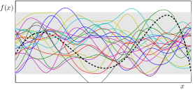
A Gaussian Process (GP) over a space $\mathcal{X}$ is a random process from $\mathcal{X}$ to $\mathbb{R}$. GPs are typically used as a prior for functions in Bayesian nonparametrics. A GP is characterised by a mean function $\mu:\mathcal{X}\rightarrow\mathbb{R}$ and a kernel (covariance function) $\kappa:\mathcal{X}^{2}\rightarrow\mathbb{R}$. If $f\sim\mathcal{G}\mathcal{P}(\mu,\kappa)$, then $f(x)$ is distributed normally $\mathcal{N}(\mu(x),\kappa(x,x))$ for all $x\in\mathcal{X}$. Some common options for the prior kernel $\kappa$ are the squared exponential and Matérn kernels. Suppose that we are given $n$ observations $\mathcal{D}_{n}=\{(x_{i},y_{i})\}_{i=1}^{n}$ from this GP, where $x_{i}\in\mathcal{X}$, $y_{i}=f(x_{i})+\epsilon_{i}\in\mathbb{R}$ and $\epsilon_{i}\sim\mathcal{N}(0,\eta^{2})$. Then the posterior $f|\mathcal{D}_{n}$ is also a GP with mean $\mu_{n}$ and covariance $\kappa_{n}$ given by,

$$\mu_{n}(x)=k^{\top}(K+\eta^{2}I_{n})^{-1}Y,\hskip 32.52127pt\kappa_{n}(x,x^{\prime})=\kappa(x,x^{\prime})-k^{\top}(K+\eta^{2}I_{n})^{-1}k^{\prime}.\hskip 3.61371pt$$ (1)

Here, $Y\in\mathbb{R}^{n}$ is a vector with $Y_{i}=y_{i}$, and $k,k^{\prime}\in\mathbb{R}^{n}$ are such that $k_{i}=\kappa(x,x_{i}),k^{\prime}_{i}=\kappa(x^{\prime},x_{i})$. $I_{n}$ is the $n\times n$ identity matrix. The Gram matrix $K\in\mathbb{R}^{n\times n}$ is given by $K_{i,j}=\kappa(x_{i},x_{j})$. We have illustrated the prior and posterior GPs in Figure 1. We refer the reader to Chapter 2 of Rasmussen and Williams (2006) for more on the basics of GPs and their use in regression.

A Review of Bayesian Optimisation:

BO refers to a suite of methods for black box optimisation in the Bayesian paradigm which use a prior belief distribution for $f$. BO methods have a common modus operandi to determine the next point ${x}_{t}$ for evaluation: first use the posterior for $f$ conditioned on the past evaluations $\{(x_{i},y_{i})\}_{i=1}^{t-1}$ to construct an acquisition function $\varphi_{t}:\mathcal{X}\rightarrow\mathbb{R}$; then maximise the acquisition to determine the next point, ${x}_{t}\in\mathop{\mathrm{argmax}}_{x\in\mathcal{X}}\varphi_{t}(x)$. At time $t$, the posterior represents our beliefs about $f$ after $t-1$ observations and $\varphi_{t}(x)$ captures the utility of performing an evaluation at $x$ according to this posterior. Typically, optimising $\varphi_{t}$ can be nontrivial. However, since $\varphi_{t}$ is analytically available, it is assumed that the effort for optimising $\varphi_{t}$ is negligible when compared to an evaluation of $f$. After $n$ evaluations of $f$, usually, the goal of an optimisation algorithm is to achieve small simple regret $S_{n}$, defined below.

$$S_{n}=f(x_{\star})-\max_{t=1,\dots,n}f(x_{t}),$$ (2)

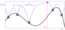
While there are several options for the prior for $f$, such as neural networks (Snoek et al., 2015; Springenberg et al., 2016) and random forests (Hutter et al., 2011), the most popular option is to use a GP. Similarly, while there are several choices for the acquisition, for the purpose of this introduction, we focus on Gaussian process upper confidence bound (GP-UCB) (Auer, 2003; Srinivas et al., 2010) and Thompson sampling (TS) (Thompson, 1933). The GP-UCB acquisition forms an upper confidence bound for $f$, and is defined as,

$$\varphi_{t}(x)\;=\mu_{t-1}(x)+\beta^{1/2}_{t}\sigma_{t-1}(x).$$ (3)

Here $\mu_{t-1}$ is the posterior mean of the GP after $t-1$ observations and is our current estimate of $f$. The posterior standard deviation, $\sigma_{t-1}$, is the uncertainty associated with this estimate. The $\mu_{t-1}$ term encourages an exploitative strategy—in that we want to query regions where we already believe $f$ is high—and $\sigma_{t-1}$ encourages an exploratory strategy—in that we want to query where we are uncertain about $f$ lest we miss high valued regions which have not been queried yet. $\beta_{t}$ controls the trade-off between exploration and exploitation. We have illustrated GP-UCB in Figure 1. Thompson sampling is another popular BO method, where at each time step, a random sample drawn from the posterior serves as the acquisition $\varphi_{t}$. Precisely, at time $t$, the next evaluation point is determined by drawing a sample $h$ from the posterior and then choosing ${x}_{t}\in\mathop{\mathrm{argmax}}_{x\in\mathcal{X}}h(x)$.

Figure 1: An illustration of GPs and BO. The first figure shows the function of interest $f$ (black line) before any observations and illustrates a GP that represents the prior uncertainty. The shaded region represents a $99\%$ confidence region for $f$ and the coloured lines are samples from the GP. The second figure shows some noisy observations (black $\times$’s) of $f$ and the posterior GP conditioned on the observations. The confidence region has shrunk around the observations. In the third figure we illustrate GP-UCB when we have to pick the next point ${x}_{t}$ given observations as shown in the second figure. The GP-UCB acquisition $\varphi_{t}$ upper bounds $f$. At time $t$, we choose the maximiser of $\varphi_{t}$ for evaluation, i.e ${x}_{t}\in\mathop{\mathrm{argmax}}_{x}\varphi_{t}(x)$.

Other common acquisitions for BO include probability of improvement (PI) (Kushner, 1964), expected improvement (GP-EI) (Jones et al., 1998), knowledge gradient (Frazier et al., 2009), top-two expected improvement TTEI (Qin et al., 2017), and entropy based methods (Hennig and Schuler, 2012).

Finally, we mention that the mean and kernel function of the prior GP have parameters which are typically chosen via empirical Bayes methods, such as maximum likelihood or posterior marginalisation; we will elaborate more on this in Section 4.2.

3 Scaling up Bayesian Optimisation

We now describe our prior work in scaling up BO to modern large scale problems. We provide only a brief overview of each method and refer the reader to the original publication for more details. Where necessary, we also provide some details on our implementation in Dragonfly.

3.1 Additive Models for High Dimensional Bayesian Optimisation

In this subsection we consider settings where $\mathcal{X}$ is a compact subset of $\mathbb{R}^{d}$. While BO has been successful in many low dimensional applications (typically $d<10$), expensive high dimensional functions occur in several fields such as computer vision (Yamins et al., 2013), antenna design (Hornby et al., 2006), computational astrophysics (Parkinson et al., 2006) and biology (Gonzalez et al., 2014). Existing theoretical and empirical results suggest that BO is exponentially difficult in high dimensions without further assumptions (Srinivas et al., 2010; Wang et al., 2013).

In Kandasamy et al. (2015a), we identify two key challenges in scaling BO to high dimensions. The first is the statistical challenge in estimating the function – nonparametric regression is inherently difficult in high dimensions (Györfi et al., 2002). The second is the computational challenge in maximising $\varphi_{t}$. Commonly used methods to maximise $\varphi_{t}$ themselves require computation exponential in dimension. We showed that we can overcome both challenges by modeling $f$ as an additive function. Prior to our work, most literature for BO in high dimensions are in the setting where the function varies only along a very low dimensional subspace (Chen et al., 2012; Wang et al., 2013; Djolonga et al., 2013). In these works, the authors do not encounter either the statistical or computational challenge as they perform BO in either a random or carefully selected lower dimensional subspace. However, these assumptions can be restrictive in many practical problems. While our additive assumption is strong in its own right, it is considerably more expressive.

Key structural Assumption: In order to make progress in high dimensions, in Kandasamy et al. (2015a), we assumed that $f$ decomposes into the following additive form,

$$f(x)=f^{(1)}(x^{(1)})+f^{(2)}(x^{(2)})+\dots+f^{(M)}(x^{(M)}).$$ (4)

Here each $x^{(j)}\in\mathcal{X}^{(j)}$ are lower dimensional groups of dimensionality $p_{j}$. In this setting, we are interested in cases where $d$ is very large and the group dimensionality is bounded: $p_{j}\leq p\ll d$. We will refer to the $\mathcal{X}^{(j)}$’s as groups and the grouping of different dimensions into these groups $\{\mathcal{X}^{(j)}\}_{j=1}^{M}$ as the decomposition. The groups are disjoint – i.e. if we treat the coordinates as a set, $x^{(i)}\cap x^{(j)}=\varnothing$. In keeping with the BO literature, we assume that each $f^{(j)}$ is sampled from a GP, $\mathcal{G}\mathcal{P}({\bf 0},\kappa^{(j)})$ where the $f^{(j)}$’s are independent. Here, $\kappa^{(j)}:\mathcal{X}^{(j)}\times\mathcal{X}^{(j)}\rightarrow\mathbb{R}$ is the kernel for $f^{(j)}$. This implies that $f$ itself is sampled from a GP with an additive kernel $\kappa(x,x^{\prime})=\sum_{j}\kappa^{(j)}(x^{(j)},{x^{(j)}}^{\prime})$. While other additive GP models have been studied before (e.g. (Duvenaud et al., 2011)), the above form will pave the way to nice computational properties, as we will see shortly.

A natural first inclination given (4) is to try GP-UCB with an additive kernel. Since an additive kernel is simpler than a $d$${}^{\textrm{th}}$ order kernel, we can expect statistical gains—in Kandasamy et al. (2015a) we showed that the regret improves from being exponential in $d$ to linear in $d$. However, the main challenge in directly using GP-UCB is that optimising $\varphi_{t}$ in high dimensions can be computationally prohibitive in practice. For example, using any grid search or branch and bound method, maximising $\varphi_{t}$ to within $\zeta$ accuracy, requires $\mathcal{O}(\zeta^{-d})$ calls to $\varphi_{t}$. To circumvent this, we proposed Add-GP-UCB which exploits the additive structure in $f$ to construct an alternative acquisition function. For this, we first describe inferring the individual $f^{(j)}$’s using observations from $f$.

Inference in additive GPs: Suppose we are given observations $Y=\{y_{1},\dots,y_{n}\}$ at $X=\{x_{1},\dots,x_{n}\}$, where $y_{i}=f(x_{i})+\epsilon$ and $\epsilon\sim\mathcal{N}(0,\eta^{2})$. For Add-GP-UCB, we will need the distribution of $f^{(j)}(x^{(j)}_{*})$ conditioned on $X,Y$, which can be shown to be the following Gaussian.

$$f^{(j)}(x^{(j)}_{*})|x_{*},X,Y\,\sim\,\mathcal{N}\big{(}{k^{(j)}}^{\top}(K+\eta^{2}I_{n})^{-1}Y\,,\kappa^{(j)}(x^{(j)}_{*},x^{(j)}_{*})-{k^{(j)}}^{\top}(K+\eta^{2}I_{n})^{-1}{k^{(j)}}\big{)}$$ (5)

where ${k^{(j)}}\in\mathbb{R}^{n}$ are such that ${k_{i}^{(j)}}=\kappa^{(j)}(x,x_{i})$. $I_{n}$ is the $n\times n$ identity matrix. The Gram matrix $K\in\mathbb{R}^{n\times n}$ is given by $K_{i,j}=\kappa(x_{i},x_{j})=\sum_{j}\kappa^{(j)}(x_{i},x_{j})$.

The Add-GP-UCB acquisition: We now define the Add-GP-UCB acquisition $\varphi_{t}$ as,

$$\varphi_{t}(x)=\sum_{j=1}^{M}\mu^{(j)}_{t-1}(x^{(j)})+\beta^{1/2}_{t}\sigma^{(j)}_{t-1}(x^{(j)}).$$ (6)

$\varphi_{t}$ can be maximised by maximising $\mu^{(j)}_{t-1}+\beta^{1/2}_{t}\sigma^{(j)}_{t-1}$ separately on $\mathcal{X}^{(j)}$. As we need to solve $M$ at most $p$ dimensional optimisation problems, it requires only $\mathcal{O}(M^{p+1}\zeta^{-p})$ calls in total to optimise within $\zeta$ accuracy—far more favourable than maximising $\varphi_{t}$.

We conclude this section with a couple of remarks. First, while our original work used a fixed group dimensionality, in Dragonfly we treat this and the decomposition as kernel parameters. We describe how they are chosen at the end of Section 5. Second, we note that several subsequent works have built on our work and studied various additive models for high dimensional BO. For example, Wang et al. (2017); Gardner et al. (2017) study methods for learning the additive structure. Furthermore, the disjointedness in our model (4) can be restrictive in applications where the function to be optimised has additive structure, but there is dependence between the variables. Some works have tried to generalise this. Li et al. (2016) use additive models with non-axis-aligned groups, and Rolland et al. (2018) study additive models with overlapping groups.

3.2 Multi-fidelity Bayesian Optimisation

Traditional methods for BO are studied in single fidelity settings; i.e. it is assumed that there is just a single expensive function $f$. However, in practice, cheap approximations to $f$ may be available. These lower fidelity approximations can be used to discard regions in $\mathcal{X}$ with low function value. We can then reserve the expensive evaluations for a small promising region. For example, in hyperparameter tuning, the cross validation curve of an expensive machine learning algorithm can be approximated via cheaper training routines using less data and/or fewer training iterations. Similarly, scientific experiments can be approximated to varying degrees using cheaper data collection and computational techniques.

BO techniques have been used in developing multi-fidelity optimisation methods in various applications such as hyperparameter tuning and industrial design (Huang et al., 2006; Swersky et al., 2013; Klein et al., 2015; Poloczek et al., 2017). However, these methods do not come with theoretical underpinnings. There has been a line of work with theoretical guarantees developing multi-fidelity methods for specific tasks such as active learning (Zhang and Chaudhuri, 2015), and model selection (Li et al., 2018). However, these papers focus on the specific applications themselves and not on general optimisation problems. In a recent line of work (Kandasamy et al., 2016c, a, b, 2017), we studied multi-fidelity optimisation and bandits under various assumptions on the approximations. To the best of our knowledge, this is the first line of work that theoretically formalises and analyses multi-fidelity optimisation. Of these, while our work in Kandasamy et al. (2016c, a, b) requires stringent assumptions on the approximations, our follow up work, BOCA  (Kandasamy et al., 2017), uses assumptions of a more Bayesian flavour and can be applied as long as we define a kernel on the approximations. We first describe the setting and algorithm for BOCA and then discuss the various modifications in our implementation in Dragonfly.

Formalism for Multi-fidelity Optimisation: We will assume the existence of a fidelity space $\mathcal{Z}$ and a function $g:\mathcal{Z}\times\mathcal{X}\rightarrow\mathbb{R}$ defined on the product space of the fidelity space and domain. The function $f$ which we wish to maximise is related to $g$ via $f(\cdot)=g(z_{\bullet},\cdot)$, where $z_{\bullet}\in\mathcal{Z}$. $z_{\bullet}$ is the fidelity at which we wish to maximise the multi-fidelity function. Our goal is to find a maximiser $x_{\star}\in\mathop{\mathrm{argmax}}_{x}f(x)=\mathop{\mathrm{argmax}}_{x}g(z_{\bullet},x)$. In the rest of the manuscript, the term “fidelities” will refer to points $z$ in the fidelity space $\mathcal{Z}$. The multi-fidelity framework is attractive when the following two conditions are true.

1. The cheap $g(z,\cdot)$ evaluation gives us information about $g(z_{\bullet},\cdot)$. As we will describe shortly, this can be achieved by modelling $g$ as a GP with an appropriate kernel for the fidelity space $\mathcal{Z}$.

2. There exist fidelities $z\in\mathcal{Z}$ where evaluating $g$ is cheaper than evaluating at $z_{\bullet}$. To this end, we will associate a known cost function $\lambda:\mathcal{Z}\rightarrow\mathbb{R}_{+}$. It is helpful to think of $z_{\bullet}$ as being the most expensive fidelity, i.e. maximiser of $\lambda$, and that $\lambda(z)$ decreases as we move away from $z_{\bullet}$. However, this notion is strictly not necessary for our algorithm or results.

We will assume $g\sim\mathcal{G}\mathcal{P}({\bf 0},\kappa)$, and upon querying at $(z,x)$ we observe $y=g(z,x)+\epsilon$ where $\epsilon\sim\mathcal{N}(0,\eta^{2})$. $\kappa:(\mathcal{Z}\times\mathcal{X})^{2}\rightarrow\mathbb{R}$ is the prior covariance defined on the product space. We will exclusively study product kernels $\kappa$ of the following form,

$$\kappa([z,x],[z^{\prime},x^{\prime}])\,=\,\kappa_{0}\,\kappa_{\mathcal{Z}}(z,z^{\prime})\,\kappa_{\mathcal{X}}(x,x^{\prime}).$$ (7)

Here, $\kappa_{0}\in\mathbb{R}_{+}$ is the scale of the kernel and $\kappa_{\mathcal{Z}},\kappa_{\mathcal{X}}$ are kernels defined on $\mathcal{Z},\mathcal{X}$ such that $\|\kappa_{\mathcal{Z}}\|_{\infty}=\|\kappa_{\mathcal{X}}\|_{\infty}=1$. This assumption implies that for any sample $g$ drawn from this GP, and for all $z\in\mathcal{Z}$, $g(z,\cdot)$ is a GP with kernel $\kappa_{\mathcal{X}}$, and vice versa. This assumption is fairly expressive – for instance, if we use an SE kernel on the joint space, it naturally partitions into a product kernel of the above form.

At time $t$, a multi-fidelity algorithm would choose a fidelity $z_{t}\in\mathcal{Z}$ and a domain point ${x}_{t}\in\mathcal{X}$ to evaluate based on its previous fidelity, domain point, observation triples $\{(z_{i},x_{i},y_{i})\}_{i=1}^{t-1}$. Here $y_{i}$ was observed when evaluating $g(z_{i},x_{i})$. Let $\mathcal{D}_{n}=\{(z_{i},x_{i},y_{i})\}_{t=1}^{n}$ be $n$ such triples from the GP $g$. We will denote the posterior mean and standard deviation of $g$ conditioned on $\mathcal{D}_{n}$ by $\nu_{n}$ and $\tau_{n}$ respectively ($\nu_{n},\tau_{n}$ can be computed from (1) by replacing $x\leftarrow[z,x]$). Denoting, $\mu_{n}(\cdot)=\nu_{n}(z_{\bullet},\cdot)$, and $\sigma_{n}(\cdot)=\tau_{n}(z_{\bullet},\cdot)$, to be the posterior mean and standard deviation of $g(z_{\bullet},\cdot)=f(\cdot)$, we have that $f|\mathcal{D}_{n}$ is also a GP and satisfies $f(x)|\mathcal{D}_{n}\sim\mathcal{N}(\mu_{n}(x),\sigma^{2}_{n}(x))$ for all $x\in\mathcal{X}$.

In Kandasamy et al. (2017), we defined both $\kappa_{\mathcal{Z}}$ and $\kappa_{\mathcal{X}}$ to be radial kernels, and proposed the following two step procedure to determine the next evaluation. At time $t$, we will first construct an upper confidence bound $\varphi_{t}$ for the function $f$ we wish to optimise. It takes the form, $\varphi_{t}(x)=\mu_{t-1}(x)+\beta^{1/2}_{t}\sigma_{t-1}(x)$, where $\mu_{t-1}$ and $\sigma_{t-1}$ are the posterior mean and standard deviation of $f$ conditioned on the observations from the previous $t-1$ time steps at all fidelities, i.e. the entire $\mathcal{Z}\times\mathcal{X}$ space. Our next point ${x}_{t}$ in the domain $\mathcal{X}$ for evaluating $g$ is a maximiser of $\varphi_{t}$, i.e.

$${x}_{t}\,\in\,\mathop{\mathrm{argmax}}_{x\in\mathcal{X}}\mu_{t-1}(x)+\beta^{1/2}_{t}\sigma_{t-1}(x)\,=\,\mathop{\mathrm{argmax}}_{x\in\mathcal{X}}\nu_{t-1}(z_{\bullet},x)+\beta^{1/2}_{t}\tau_{t-1}(z_{\bullet},x).$$ (8)

We then choose $z_{t}=\mathop{\mathrm{argmin}}_{z\in\mathcal{Z}_{t}({x}_{t})}\lambda(z)$ where,

$$\mathcal{Z}_{t}({x}_{t})=\{z_{\bullet}\}\cup\left\{z:\lambda(z)<\lambda(z_{\bullet}),\;\tau_{t-1}(z,{x}_{t})>\sqrt{\kappa_{0}}\xi(z)\sqrt{\lambda(z)/\lambda(z_{\bullet})}\right\}.$$ (9)

Here $\xi(z)$ is an information gap function. We refer the reader to Section 2 in Kandasamy et al. (2017) for the definition and more details on $\xi(z)$, but intuitively, it measures the price we have to pay, in information, for querying away from $z_{\bullet}$. $\xi(z)$ is a well defined quantity for radial kernels; for e.g. for kernels of the form $\kappa(z,z^{\prime})=\exp(\|z-z^{\prime}\|^{2\gamma})$, one can show that $\xi(z)$ is approximately proportional to $\|z-z_{\bullet}\|^{\gamma}$. The second step in BOCA says that we will only consider fidelities where the posterior variance is larger than a threshold. This threshold captures the trade-off between cost and information in the approximations available to us; cheaper fidelities cost less, but provide less accurate information about the function $f$ we wish to optimise.

Other acquisitions: A key property about the criterion (9) shown in Kandasamy et al. (2017), is that is chooses a fidelity $z_{t}$ with good cost to information trade-off, given that we are going to evaluate $g$ at ${x}_{t}$. In particular, it applies to ${x}_{t}$ chosen in an arbitrary fashion, and not necessarily via an upper confidence bound criterion (8). Therefore in Dragonfly, we adopt the two step procedure described above, but allow ${x}_{t}$ to be chosen also via other acquisitions as well.

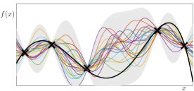
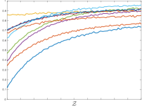
Exponential decay kernels for monotonic approximations: In Kandasamy et al. (2017), we choose the fidelity kernel $\kappa_{\mathcal{Z}}$ to be a radial kernel. This typically induces smoothness in $g$ across $\mathcal{Z}$, which can be useful in many applications. However, in model selection, the approximations are obtained by using less data and/or less iterations in an iterative training procedure. In such cases, as we move to the expensive fidelities, the validation performance tends to be monotonic—for example, when the size of the training set increases, one expects the validation accuracy to keep improving. Swersky et al. (2014b) demonstrated that an exponential decay kernel $\kappa_{\textrm{ed}}(u,u^{\prime})=1/(u+u^{\prime}+1)^{\alpha}$, can strongly support such sample paths. We have illustrated such sample paths in Figure 2. In a $p$ dimensional fidelity space, one can use $\kappa_{\mathcal{Z}}(z,z^{\prime})=\prod_{i=1}^{p}\kappa_{\textrm{ed}}(z_{i},z_{i}^{\prime})$ as the kernel for the fidelity space if all fidelity dimensions exhibit such behaviour. Unfortunately, the information gain $\xi(z)$ is not defined for non-radial kernels. In Dragonfly, we use $\xi(z)=\|z-z_{\bullet}\|$ which is similar to the approximation of the information gain for SE kernels. Intuitively, as $z$ moves away from $z_{\bullet}$, the information gap increases as $g(z,\cdot)$ provides less information about $g(z_{\bullet},\cdot)$.

Figure 2: An illustration of GP sample paths drawn from the exponential decay kernel (Swersky et al., 2014b) conditioned on being positive. They are suitable for representing the validation accuracy along a fidelity dimension in model selection where, for e.g. validation accuracy tends to increase as we use more data and/or train for more iterations.

This concludes our description of multi-fidelity optimisation in Dragonfly. Following our work, there have been a few papers on multi-fidelity optimisation with theoretical guarantees. Sen et al. (2018a, b) develop an algorithm in frequentist settings which builds on the key intuitions here, i.e. query at low fidelities and proceed higher only when the uncertainty has shrunk. In addition, Song et al. (2019) develop a Bayesian algorithm which chooses fidelities based on the mutual information.

3.3 Bayesian Optimisation for Neural Architecture Search

In this section, we study using BO for neural architecture search (NAS), i.e. for finding the optimal neural network architecture for a given prediction problem. The majority of the BO literature has focused on settings where the domain $\mathcal{X}$ is either Euclidean and/or categorical. However, with the recent successes of deep learning, neural networks are increasingly becoming the method of choice for many machine learning applications. Recent work has demonstrated that architectures which deviate from traditional feed forward structures perform welle.g. He et al. (2016); Huang et al. (2017). This motivates studying model selection methods which search the space of neural architectures and optimise for generalisation performance. While there has been some work on BO for architecture search (Swersky et al., 2014a; Mendoza et al., 2016), they only optimise among feed forward architectures. Jenatton et al. (2017) study methods for BO in tree structured spaces, and demonstrate an application in optimising feed forward architectures. Besides BO, other techniques for NAS include reinforcement learning (Zoph and Le, 2017), evolutionary algorithms (Liu et al., 2017), gradient based methods (Liu et al., 2019), and random search (Li and Talwalkar, 2019).

There are two main challenges for realising GP based BO for architecture search where each element $x\in\mathcal{X}$ in our domain is now a neural network architecture. First, we must quantify the similarity between two architectures $x,x^{\prime}$ in the form of a kernel $\kappa(x,x^{\prime})$. Secondly, we must maximise $\varphi_{t}$, the acquisition function, in order to determine which point $x_{t}$ to test at time $t$. To tackle these issues, in Kandasamy et al. (2018b) we develop a (pseudo-) distance for neural network architectures called OTMANN (Optimal Transport Metrics for Architectures of Neural Networks) that can be computed efficiently via an optimal transport program. Using this distance, we develop a BO framework for optimising functions defined on neural architectures called NASBOT (Neural Architecture Search with Bayesian Optimisation and Optimal Transport), which we describe next. We will only provide high level details and refer the reader to Kandasamy et al. (2018b) for a more detailed exposition.

The OTMANN Distance and Kernel: Our first and primary contribution in Kandasamy et al. (2018b) was to develop a distance metric $d$ among neural networks; given a distance $d$ of this form, we may use $e^{-\beta d}$ as the kernel. This distance was designed taking into consideration the fact that the performance of an architecture is determined by the amount of computation at each layer, the types of these operations, and how the layers are connected. A meaningful distance should account for these factors. To that end, OTMANN is defined as the minimum of a matching scheme which attempts to match a notion of mass at the layers from one network to the layers of the other. The mass is proportional to the amount of computation happening at each layer. We incur penalties for matching layers with different types of operations or those at structurally different positions. The goal is to find a matching that minimises these penalties, and the penalty at the minimum is a measure of dissimilarity between two networks $\mathcal{G}_{1},\mathcal{G}_{2}$. In Kandasamy et al. (2018b), we show that this matching scheme can be formulated as an optimal transport program (Villani, 2003), and moreover the solution induces a pseudo-distance $d$ in the space of neural architectures.

The NASBOT Algorithm and its implementation in Dragonfly: Equipped with such a distance, we use a sum of exponentiated distance terms as the kernel, as explained previously. These distances are obtained via different parameters of OTMANN and/or via normalised versions of the original distance. To optimise the acquisition, we use an evolutionary algorithm. For this, we define a library of modifiers which modify a given network by changing the number of units in a layer, or make structural changes such as adding skip connections, removing/adding layers, and adding branching (see Table 6 in Kandasamy et al. (2018b)). The modifiers allow us to navigate the search space, and the evolutionary strategy allows us to choose good candidates to modify. In Dragonfly, we also tune for the learning rate, and moreover, allow for multi-fidelity optimisation, allowing an algorithm to train a model partially and observe its performance. We use the number of training batch iterations as a fidelity parameter and use an exponential decay kernel across the fidelity space.

3.4 Parallelisation

BO, as described in Section 2, is a sequential algorithm which determines the next query after completing previous queries. However, in many applications, we may have access to multiple workers and hence carry out several evaluations simultaneously. As we demonstrated theoretically in Kandasamy et al. (2018a), when there is high variability in evaluation times, it is prudent for BO to operate in an asynchronous setting, where a worker is re-deployed immediately with a new evaluation once it completes an evaluation. In contrast, if all evaluations take roughly the same amount of time, it is meaningful to wait for all workers to finish, and incorporate all their feedback before issuing the next set of queries in batches.

In our implementations of all acquisitions except TS, we handle parallelisation using the hallucination technique of Desautels et al. (2014); Ginsbourger et al. (2011). Here, we pick the next point exactly as in the sequential setting, but the posterior is based on $\mathcal{D}_{t}\cup\{(x,\mu_{t-1}(x))\}_{x\in F_{t}}$, where $F_{t}$ are the points in evaluation by other workers at step $t$ and $\mu_{t-1}$ is the posterior mean conditioned on just $\mathcal{D}_{t}$. This preserves the mean of the GP, but shrinks the variance around the points in $F_{t}$, thus discouraging the algorithm from picking points close to those that are in evaluation. However, for TS, as we demonstrated in Kandasamy et al. (2018a), a naive application would suffice, as the inherent randomness of TS ensures that the points chosen for parallel evaluation are sufficiently diverse. Therefore, Dragonfly does not use hallucinations for TS. While there are other techniques for parallelising BO, they either require choosing additional parameters and/or are computationally expensive (González et al., 2016; Shah and Ghahramani, 2015; Wang et al., 2018).

4 Robust Bayesian Optimisation in Dragonfly

We now describe our design principles for robust GP based BO in Dragonfly. We favour randomised approaches which uses multiple acquisitions and GP hyperparameter values at different iterations since we found them to be quite robust in our experiments.

4.1 Choice of Acquisition

Figure 3: Comparison of using individual acquisitions such as GP-UCB, GP-EI, TTEI, TS, PI, and Add-GP-UCB versus the combined sampling method as described in Section 4.1. We have also shown random sampling (RAND) for comparison. We plot the simple regret (2), so lower is better. Error bars indicate one standard error. All curves were produced by averaging over $10$ independent runs.

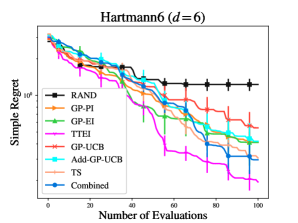
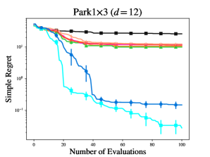
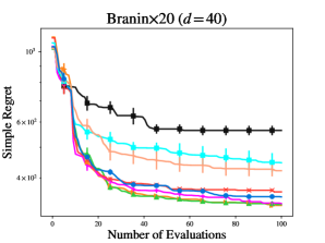
Dragonfly implements several common acquisitions for BO such as GP-UCB, GP-EI, TTEI, TS, Add-GP-UCB, and PI. The general practice in the BO literature has been for a practitioner to pick their favourite acquisition, and use it for the entire optimisation process. However, the performance of each acquisition can be very problem dependent, as demonstrated in Figure 3. Therefore, instead of trying to pick the single best acquisition, we adopt an adaptive sampling strategy which chooses different acquisitions at different iterations instead of attempting to pick a single best one.

Our sampling approach maintains a list of $m$ acquisitions $\ell^{\textrm{acq}}$ along with a weight vector $w^{\textrm{acq}}_{t}=$ $\{w^{\textrm{acq}}_{t}[\alpha]\}_{\alpha\in\ell^{\textrm{acq}}}$ $\in\mathbb{R}^{m}$. We set $w^{\textrm{acq}}_{0}[\alpha]=\omega^{\textrm{acq}}_{0}$ for all $\alpha\in\ell^{\textrm{acq}}$. Suppose at time step $t$, we chose acquisition $\theta$ and found a higher $f$ value than the current best value. We then update $w^{\textrm{acq}}_{t+1}[\alpha]\leftarrow w^{\textrm{acq}}_{t}[\alpha]+\mathbbm{1}(\theta=\alpha)$; otherwise, $w^{\textrm{acq}}_{t+1}[\alpha]\leftarrow w^{\textrm{acq}}_{t}[\alpha]$. At time $t$, we choose acquisition $\theta\in\ell^{\textrm{acq}}$ with probability $w^{\textrm{acq}}_{t}[\theta]/\sum_{\alpha}w^{\textrm{acq}}_{t}[\alpha]$. This strategy initially samples all acquisitions with equal probability, but progressively favours those that perform better on the problem.

By default, we set $\ell^{\textrm{acq}}=\{\text{{{GP-UCB}}, {{GP-EI}}, {{TS}}, {{TTEI}}}\}$; for entirely Euclidean domains, we also include Add-GP-UCB. We do not incorporate PI since it consistently underperformed other acquisitions in our experiments. As Figure 3 indicates, the combined approach is robust across different problems, and is competitive with the best acquisition on the given problem. A similar sampling approach to ours is used in Hoffman et al. (2011). Shahriari et al. (2014) use an entropy based approach to select among multiple acquisitions; however, this requires optimising all of them which can be expensive. We found that our approach, while heuristic in nature, performed well in our experiments. Finally, we note that we do not implement entropy based acquisitions, since their computation can, in general, be quite expensive.

4.2 GP Hyperparameters

One of the main challenges in GP based BO is that the selection of the GP hyperparameters themselves could be notoriously difficult. While a common approach is to choose them by maximising the marginal likelihood, in some cases, this could also cause overfitting in the GP, especially in the early iterations (Snoek et al., 2012). The most common strategy to overcome this issue is to maintain a prior on the hyperparameters and integrate over the posterior (Malkomes et al., 2016; Snoek et al., 2012; Hoffman and Shahriari, 2014). However, this can be very computationally burdensome, and hence prohibitive in applications where function evaluations are only moderately expensive. Instead, in this work, we focus on a different approach that uses posterior sampling. Precisely, at each iteration, one may sample a set of GP hyperparameters from the posterior conditioned on the data, and use them for the GP at that iteration. Intuitively, this is similar to a Thompson sampling procedure where the prior on the hyperparameters specifies a prior on a meta-model, and once we sample the hyperparameters, we use an acquisition of our choice. When this acquisition is TS, this procedure is exactly Thompson sampling using the meta-prior.

Our experience suggested that maximising the marginal likelihood (ML) generally worked well in settings where the function was smooth; for less smooth functions, sampling from the posterior (PS) tended to work better. We speculate that this is because, with smooth functions, a few points are sufficient to estimate the landscape of the function, and hence maximum likelihood does not overfit; since it has already estimated the GP hyperparameters well, it does better than PS. On the other hand, while ML is prone to overfit for non-smooth functions, the randomness in PS prevents us from getting stuck at bad GP hyperparameters. As we demonstrate in Figure 4, either of these approaches may perform better than the other depending on the problem.

Figure 4: Comparison using only maximum likelihood (ML), only posterior sampling (PS) and the combined sampling approach (ML+PS) as described in Section 4.2. We have also shown random sampling (RAND) for comparison. We plot the simple regret (2), so lower is better. All curves were produced by averaging over $10$ independent runs. Error bars indicate one standard error.

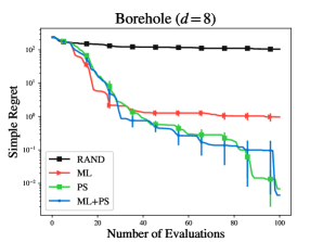
Therefore, similar to how we handled the acquisitions, we adopt a sampling approach where we choose either maximum likelihood or sampling from the posterior at every iteration. Our GP hyperparameter tuning strategy proceeds as follows. After every $n_{{\textrm{cyc}}}$ evaluations of $f$, we fit a single GP to it via maximum likelihood, and also sample $n_{{\textrm{cyc}}}$ hyperparameter values from the posterior. At every iteration, the algorithm chooses either ML or PS in a randomised fashion. If it chooses the former, it uses the single best GP, and if it chooses the latter, it uses one of the sampled values. For the sampling strategy, we let $w^{\textrm{hp}}_{t}=\{w^{\textrm{hp}}_{t}[h]\}_{h\in\ell^{\textrm{hp}}}\in\mathbb{R}^{2}$ where $\ell^{\textrm{hp}}=\{\text{{{ML}}, {{PS}}}\}$ and choose strategy $h\in\ell^{\textrm{hp}}$ with probability $w^{\textrm{hp}}_{t}[h]/(w^{\textrm{hp}}_{t}[\text{{{ML}}}]+w^{\textrm{hp}}_{t}[\text{{{PS}}}])$. We update $w^{\textrm{hp}}_{t}$ in a manner similar to $w^{\textrm{acq}}_{t}$. Figure 4 demonstrates that this strategy performs as well as, if not better than the best of ML and PS.

By default, Dragonfly uses $n_{{\textrm{cyc}}}=17$. For maximum likelihood of continuous GP hyperparameters, we use either DiRect (Jones et al., 1993) or PDOO (Grill et al., 2015). If discrete hyperparameters are also present, we optimise the continuous parameters for all choices of discrete values; this is feasible, since, in most cases, there are only a handful of discrete GP hyperparameter values. For posterior sampling, we impose a uniform prior and use Gibbs sampling as follows. At every iteration, we visit each hyperparameter in a randomised order; on each visit, we sample a new value for the current hyperparameter, conditioned on the values of the rest of the hyperparameters. For continuous hyperparameters, we do so via slice sampling (Neal, 2003) and, for discrete hyperparameters, we use Metropolis-Hastings. We use a burn-in of $1000$ samples and collect a sample every $100$ samples from thereon to avoid correlation. Next, we describe our BO implementation in Dragonfly.

5 BO Implementation in Dragonfly

Domains: Dragonfly allows optimising over domains with Euclidean, integral, and discrete variables. We also define discrete numeric and discrete Euclidean variable types, where a variable can assume one of a finite discrete set of real numbers and Euclidean vectors respectively. We also allow neural network variable types which permits us to optimise functions over neural network architectures. In addition to specifying variables, one might wish to impose constraints on the allowable values of these variables. These constraints can be specified via a Boolean function which takes a point and returns True if and only if the point exists in the domain. For example, if we have a Euclidean variable $x\in[-1,1]^{2}$, the function $\mathbbm{1}\{\|x\|_{2}\leq 1\}$ constrains the domain to the unit ball. In Dragonfly, these constraints can be specified via a Python expression or function.

Kernels: For Euclidean, integral, and discrete numeric variables, Dragonfly implements the squared exponential and Matérn kernels. We also implement additive variants of above kernels for the Add-GP-UCB acquisition. Following recommendations in Snoek et al. (2012), we use the Matérn-2.5 kernel by default for above variable types. We found that it generally performed better across our experiments as well. For discrete variables, we use the Hamming kernel (Hutter et al., 2011); precisely, given $x,x^{\prime}\in\times_{i=1}^{k}A_{i}$, where each $A_{i}$ is a discrete domain, we use $\kappa_{\sigma,\alpha}(x,x^{\prime})=\sigma\sum_{i=1}^{k}\alpha_{i}\mathbbm{1}(x_{i}=x^{\prime}_{i})$ as the kernel. Here $\sigma>0$ and $\alpha\in\mathbb{R}_{+}^{k}$, $\sum_{i}\alpha_{i}=1$ are kernel hyperparameters determining the scale and the relative importance of each discrete variable respectively. Dragonfly also implements the OTMANN and exponential decay kernels discussed in Sections 3.3 and 3.2 respectively.

Optimising the Acquisition: To maximise the acquisition $\varphi_{t}$ in purely Euclidean spaces with no constraints, we use DiRect (Jones et al., 1993) or PDOO (Grill et al., 2015), depending on the dimensionality $d$. Our Fortran implementation of DiRect, can only handle up to $d=64$; for larger dimensions we use PDOO. In all other cases, we use an evolutionary algorithm. For this, we begin with an initial pool of randomly chosen points in the domain and evaluate the acquisition at those points. We then generate a set of $N_{\textrm{mut}}$ mutations of this pool as follows; first, stochastically select $N_{\textrm{mut}}$ candidates from this set such that those with higher $\varphi_{t}$ values are more likely to be selected; then apply a mutation operator to each candidate. Then, we evaluate the acquisition on this $N_{\textrm{mut}}$ mutations, add it to the initial pool, and repeat for the prescribed number of steps. We choose an evolutionary algorithm since it is simple to implement and works well for cheap functions, such as the acquisition $\varphi_{t}$. However, as we demonstrate in Section 6, it is not ideally suited for expensive-to-evaluate functions. Each time we generate a new candidate we test if they satisfy the constraints specified. If they do not, we reject that sample and keep sampling until all constraints are satisfied. One disadvantage to this rejection sampling procedure is that if the constrains only permit a small subset of the entire domain, it could significantly slow down the optimisation of the acquisition.

Initialisation: We bootstrap our BO routine with $n_{{\textrm{init}}}$ evaluations. For Euclidean and integral variables, these points are chosen via latin hypercube sampling, while for discrete and discrete numeric variables they are chosen uniformly at random. For neural network variables, we choose $n_{{\textrm{init}}}$ feed forward architectures. Once sampled, as we did when optimising the acquisition, we use rejection sampling to test if the constraints on the domain are satisfied. By default, $n_{{\textrm{init}}}$ is set to $5d$ where $d$ is the dimensionality of the domain but is capped off at $7.5\%$ of the optimisation budget.

We have summarised the resulting procedure for BO in Dragonfly in Algorithm 1. $q,q^{\prime}$ denote a query. In usual BO settings, they simply refer to the next point $x\in\mathcal{X}$, i.e. $q=(x)$; in multi-fidelity settings they also include the fidelity $z\in\mathcal{Z}$, i.e. $q=(z,x)$. $\textrm{acq}(q),\textrm{hp}(q)$ refer to the acquisition and the choice of {ML, PS} for GP parameter selection. $\textrm{multinomial-sample}(\ell,w)$ samples an element from a set $\ell$ from the multinomial distribution $\{w_{i}/\sum_{j}w_{j}\}_{i=1}^{|\ell|}$. Before concluding this section, we take a look at two implementation details for Add-GP-UCB.

0:  $n_{{\textrm{init}}}$, $n_{{\textrm{cyc}}}$, $\ell^{\textrm{acq}}$, $\ell^{\textrm{hp}}$.

1:  $\mathcal{D}_{0}\leftarrow$ Evaluate $f$ at $n_{{\textrm{init}}}$ points.

2:  $y_{\textrm{max}}\leftarrow$ maximum $y$ value in $\mathcal{D}_{0}$.

3:  $w^{\textrm{acq}}=\omega^{\textrm{acq}}_{0}{\bf 1}_{|\ell^{\textrm{acq}}|}$.

4:  $w^{\textrm{hp}}=\omega^{\textrm{hp}}_{0}{\bf 1}_{2}$.

5:  for $j=0,1,2\dots$ do

6:     Wait for a worker to finish.

7:     $\mathcal{D}_{j}\leftarrow\mathcal{D}_{j-1}\cup\{(q,y)\}$ where $(q,y)$ are the worker’s previous query and observation.

8:     if $y>y_{\textrm{max}}$, then # update weights if new max-value was found

9:        $w^{\textrm{acq}}[\textrm{acq}(q)]=w^{\textrm{acq}}[\textrm{acq}(q)]+1$.

10:        $w^{\textrm{hp}}[\textrm{hp}(q)]=w^{\textrm{hp}}[\textrm{hp}(q)]+1$.

11:     end if

12:     if $\mod(t,n_{{\textrm{cyc}}})=0$,  then # updates for GP hyperparameters

13:        $\Theta^{\text{{{PS}}}}\leftarrow$ sample $n_{{\textrm{cyc}}}$ GP hyperparameter values.

14:        $\theta^{\text{{{ML}}}}\leftarrow$ maximise GP marginal likelihood to find best GP hyperparameter values.

15:     end if

16:     $\theta\leftarrow\textrm{multinomail-sample}([\textrm{pop}(\Theta),\theta^{\text{{{ML}}}}],w^{\textrm{hp}})$. # choose GP hyperparameters

17:     $\alpha\leftarrow\textrm{multinomial-sample}(\ell^{\textrm{acq}},w^{\textrm{acq}})$. # choose acquisition

18:     $\mu_{t-1}\leftarrow$ Compute posterior GP mean given $\mathcal{D}_{j}$ using $\theta$.

19:     Compute hallucinated posterior GP $\mathcal{G}\mathcal{P}_{t-1}\leftarrow\mathcal{G}\mathcal{P}(\mu_{t-1},\kappa_{t-1};\mathcal{D}_{j}\cup\{(x,\mu_{t-1}(x))\}_{x\in F_{t}},\theta)$.

20:     $q^{\prime}\leftarrow$ Determine next query for evaluation using acquisition $\alpha$ and GP $\mathcal{G}\mathcal{P}_{t-1}$.

21:     Re-deploy worker with an evaluation at $q^{\prime}$.

22:  end for

Algorithm 1  Bayesian Optimisation in Dragonfly with $M$ asynchronous workers

Choosing the decomposition for Add-GP-UCB: Recall from Section 3.1, the additive decomposition and maximum group dimensionality for Add-GP-UCB are treated as kernel parameters. We conclude this section by describing the procedure for choosing these parameters, both for ML and PS. For the former, since a complete maximisation can be computationally challenging, we perform a partial maximisation by first choosing an upper bound $p_{\textrm{max}}$ for the maximum group dimensionality. For each group dimensionality $p\in\{1,\dots,p_{\textrm{max}}\}$, we select $k$ different decompositions chosen at random. For each such decomposition, we optimise the marginal likelihood over the remaining hyperparameters, and choose the decomposition with the highest likelihood. For PS, we use the following prior for Gibbs sampling. First, we pick the maximum group dimensionality $p$ uniformly from $\{1,\dots,p_{\textrm{max}}\}$. We then randomly shuffle the coordinates $\{1,\dots,d\}$ to produce an ordering. Given a maximum group dimensionality $p$ and an ordering, one can uniquely identify a decomposition by iterating through the ordering and grouping them in groups of size at most $p$. For example, in a $d=7$ dimensional problem, $p=3$ and the ordering $4,7,3,6,1,5,2$ yields the decomposition $\{(3,4,7),(1,5,6),(2)\}$ of three groups having group dimensionalities 3, 3, and 1 respectively.

Since the set of possible decompositions is a large combinatorial space, we might not be able to find the true maximiser of the marginal likelihood in ML or cover the entire space via sampling in PS. However, we adopt a pragmatic view of the additive model (4) which views it as a sensible approximation to $f$ in the small sample regime, as opposed to truly believing that $f$ is additive. Under this view, we can hope to recover any existing marginal structure in $f$ via a partial maximisation or a few posterior samples. In contrast, an exhaustive search may not do much better when there is no additive structure. By default, Dragonfly uses $p_{\textrm{max}}=6$ and $k=25$ for Add-GP-UCB.

Combining multi-fidelity with Add-GP-UCB: When using an additive kernel $\kappa_{\mathcal{X}}=\sum_{j}\kappa^{(j)}$ for the domain $\mathcal{X}$ in multi-fidelity settings, the resulting product kernel also takes an additive form, $\kappa([z,x],[z^{\prime},x^{\prime}])=\sum_{j}\kappa_{\mathcal{Z}}(z,z^{\prime})\kappa(x^{(j)},{x^{(j)}}^{\prime})$. When using Add-GP-UCB, in the first step we choose $x^{(j)}_{t}\in\mathop{\mathrm{argmax}}_{x^{(j)}\in\mathcal{X}^{(j)}}$ $\nu_{t-1}^{(j)}(z_{\bullet},x^{(j)})+\beta^{1/2}_{t}\tau_{t-1}^{(j)}(z_{\bullet},x^{(j)})$ for all $j$ to obtain the next evaluation ${x}_{t}$. Here $\nu_{t-1}^{(j)},\tau_{t-1}^{(j)}$ are the posterior GP mean and standard deviation of the $j$${}^{\textrm{th}}$ function in the above decomposition. Then we choose the fidelity $z_{t}$ as described in (9).

6 Experiments

We now compare Dragonfly to the following algorithms and packages. RAND: uniform random search; EA: evolutionary algorithm; PDOO: parallel deterministic optimistic optimisation (Grill et al., 2015); HyperOpt (v0.1.1) (Bergstra et al., 2013); SMAC (v0.9.0) (Hutter et al., 2011); Spearmint (Snoek et al., 2012); GPyOpt (v1.2.5) (Authors, 2016). Of these PDOO is a deterministic non-Bayesian algorithm for Euclidean domains. SMAC, Spearmint, and GPyOpt are model based BO procedures, where SMAC uses random forests, while Spearmint and GPyOpt use GPs. For EA, we use the same procedure used to optimise the acquisition in Section 5. We begin with experiments on some standard synthetic benchmarks for zeroth order optimisation.

6.1 Experiments on Synthetic Benchmarks

Figure 5: Comparison of Dragonfly with other algorithms and BO packages on functions with noiseless evaluations defined on Euclidean domains. We plot the simple regret (2) so lower is better. The title states the name of the function, and its dimensionality. All curves were produced by averaging over $20$ independent runs. Error bars indicate one standard error. The legend for all curves is available in the first figure. SMAC’s initialisation procedure did not work in dimensions larger than $40$ so it is not shown in the respective figures. Spearmint is not shown on all figures since it was too slow to run on high dimensional problems.

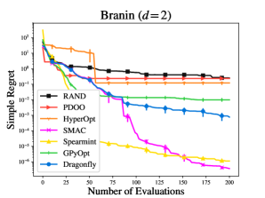
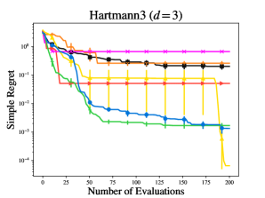
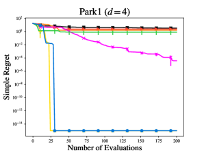
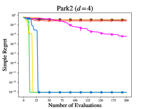
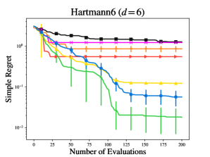
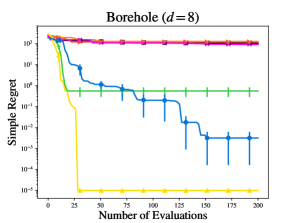
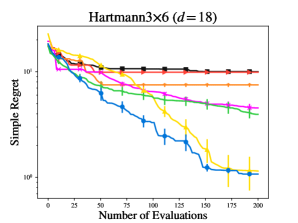
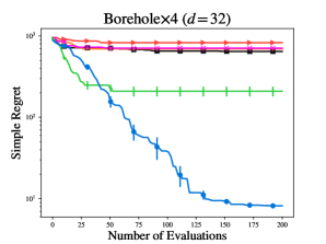
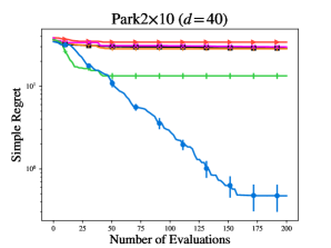
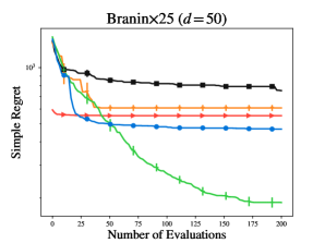
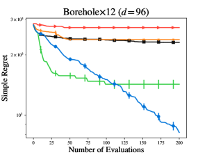
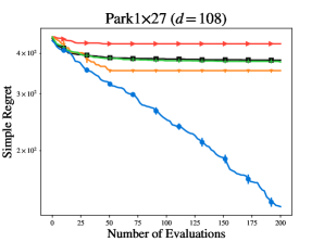
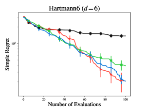
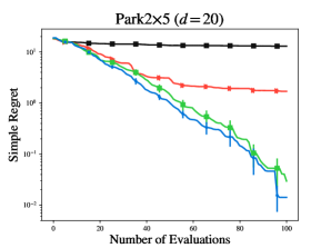
Euclidean Domains: Our first set of experiments are on a series of synthetic benchmarks in Euclidean domains. We use the Branin $(d=2)$, Hartmann3 $(d=3)$, Park1 $(d=4)$, Park2 $(d=4)$, Hartmann6 $(d=6)$, and Borehole $(d=8)$ benchmarks, and additionally, construct high dimensional versions of the above benchmarks. The high dimensional forms were obtained via an additive model $f(x)=f^{\prime}(x^{(1)})+f^{\prime}(x^{(2)})\dots$ where $f^{\prime}$ is a lower dimensional function and the $x^{(i)}$’s are coordinates forming a low dimensional subspace. For example, in the Hartmann3x6 problem, we have an $18$ dimensional function obtained by considering six Hartmann3 functions along coordinate groups $\{1,2,3\},\{4,5,6\},\dots,\{16,17,18\}$. We compare all methods on their performance over $200$ evaluations. The results are given in Figure 5, where we plot the simple regret (2) against the number of evaluations (lower is better). As its performance was typically worse than all other BO methods, we do not compare to EA to avoid clutter in the figures. Spearmint is not shown on the higher dimensional problems since it was too slow beyond 25-30 dimensions. SMAC’s initialisation procedure failed in dimensions larger than $40$ and is not shown in the corresponding experiments.

Figure 6: Comparison of Dragonfly with other algorithms and BO packages on synthetic functions defined on non-Euclidean domains. We plot the maximum value, so higher is better. The $x$-axis shows the expended capital and the $y$ axis is the maximum value (higher is better). The title states the name of the function, and its dimensionality (number of variables). We do not state the dimensionality for the synthetic CNN function since the dimensionality of a space of CNN architectures is not defined. All curves were produced by averaging over $20$ independent runs. Error bars indicate one standard error. The legend for all curves is available in the first figure. We do not compare Spearmint, HyperOpt, SMAC, and GPyOpt on the synthetic CNN function since they do not support optimising over neural architectures.

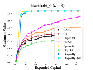
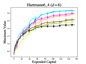
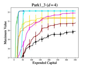
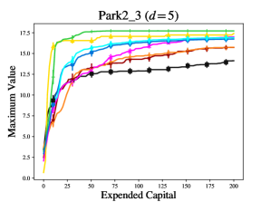
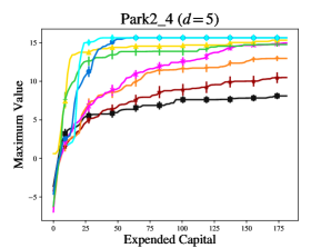
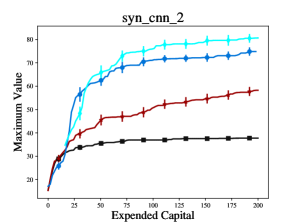
Non-Euclidean Domains: Next, we compare Dragonfly to the above baselines on non-Euclidean domains. For this, we modify the above benchmarks, originally defined on Euclidean domains, so that they can take non-Euclidean arguments. Specifically, we use modified versions of the Borehole, Hartmann6, Park1 and Park2 functions. We also construct a synthetic function defined on CNN architectures, on a synthetic NAS problem. The results are given in Figure 6. Since the true maxima of these functions are not known, we simply plot the maximum value found against the number of evaluations (higher is better). In this set of experiments, in addition to vanilla BO, we also construct variations of these function which can take a fidelity argument. Hence, a strategy may use these approximations to speed up the optimisation process. The $x$-axis in all cases refers to the expended capital, which was chosen so that a single fidelity algorithm would perform exactly 200 evaluations. We compare a multi-fidelity version of Dragonfly, which uses the BOCA strategy (Kandasamy et al., 2017), to choose the fidelities and points for evaluation. See github.com/dragonfly/dragonfly/tree/master/examples/synthetic for a description of these functions and the approximations for the multi-fidelity cases.

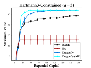
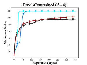
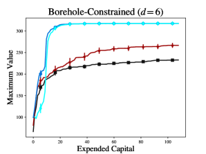
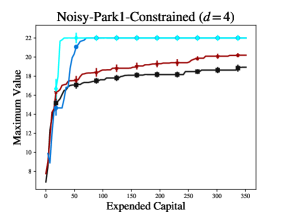
Domains with Constraints: Next, we consider three optimisation tasks where we impose additional constraints on the domain variables. Specifically, we consider versions of the Hartmann3, Park1 and Borehole functions. As an example, the Hartmann3 function is usually defined on the domain $[0,1]^{3}$; however, we consider a constrained domain $\mathcal{X}=\big{\{}x\in[0,1]^{3}\,;\,x_{1}^{2}+x_{2}^{2}\leq 1/2\big{\}}$. Descriptions of the other functions and domains are available in the Dragonfly repository. In Figure 7, we compare Dragonfly to RAND and EA. We do not compare to other methods and packages, since, to our knowledge, they cannot handle arbitrary constraints of the above form.

Figure 7: Comparison of Dragonfly with RAND and EA on synthetic functions with constraints on the domain. See caption under Figure 6 for more details.

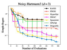
Noisy Evaluations: Finally, we compare all methods when evaluations are noisy. We use 6 test functions from above, but add Gaussian noise to each evaluation; the width of the Gaussian was chosen based on the range of the function. We evaluate all methods on the maximum true function value queried (as opposed to the observed maximum value). The results are given in Figure 8.

Figure 8: Experiments on synthetic functions when evaluations are noisy. In the top row, the domain is Euclidean and we plot the number of evaluations versus simple regret (lower is better). In the bottom row, the domain is non-Euclidean, and we plot the expended capital versus the maximum true value found (higher is better). The legend for each row is given in the leftmost figure. See captions under Figures 5, 6, and 7 for more details.

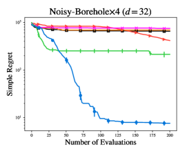
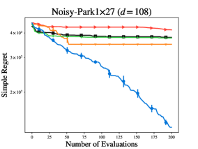
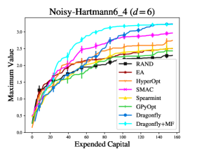
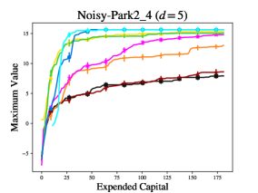
Take-aways: On Euclidean domains, Spearmint and Dragonfly perform consistently well across the lower dimensional tasks, but Spearmint is prohibitively expensive in high dimensions. On the higher dimensional tasks, Dragonfly is the most competitive. It is worth pointing out that on the Park1 and Park2 benchmarks, Dragonfly and Spearmint do significantly better than other methods. We believe this is because these packages have discovered a good but hard to find optimum on these problems, whereas other packages have only discovered worse local optima. On non-Euclidean domains, we see that Dragonfly is able to do consistently well. GPyOpt and Dragonfly perform very well on some problems, but also perform poorly on others. It is interesting to note that the improvements due to multi-fidelity optimisation are modest in some cases. We believe this is due to two factors. First, the multi-fidelity method spends an initial fraction of its capital at the lower fidelities, and the simple regret is $\infty$ until it queries the highest fidelity. Second, there is an additional statistical difficulty in estimating, what is now a more complicated GP model across the domain and fidelity space. We have summarised the results on the synthetic experiments in Table 1 separately for the Euclidean and non-Euclidean synthetic benchmarks. These include the results in Figures 5, 6, and 8. We exclude the constrained optimisation results from Figure 7 since there are too few baselines in this setting. From these results, we see that Dragonfly performs consistently well across a wide range of benchmarks.

6.2 Experiments on Astrophysical Maximum Likelihood Problems

In this section, we consider two maximum likelihood problems in computational Astrophysics.

Method	Dragonfly	GPyOpt	Spearmint	SMAC	HyperOpt	PDOO	RAND	EA
Euclidean	8-5-2-0	3-3-4-2	3-3-3-0	1-0-3-2	0-3-0-2	0-0-3-4	0-0-1-5	N/A
Non-Euclidean	5-2-0-1	2-0-1-1	1-3-0-2	0-2-4-1	0-0-2-1	N/A	0-0-1-0	0-1-0-1

Table 1: A summary of the ranks of each method on the Euclidean and non-Euclidean synthetic problems at the end of $200$ evaluations. We show the number of times each method was ranked within the first four in the order $n1-n2-n3-n4$ where $<nk>$ is the number of times the method was ranked $k$${}^{\textrm{th}}$ in the problems. There are a total of 15 Euclidean problems (12 from Figure 5, 3 from Figure 8) and 8 non-Euclidean problems (6 from Figure 6, 2 from Figure 8). We exclude the multi-fidelity methods from this table.

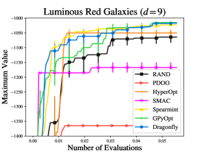
Luminous Red Galaxies: Here we used data on Luminous Red Galaxies (LRGs) for maximum likelihood inference on 9 Euclidean cosmological parameters. The likelihood is computed via the galaxy power spectrum. Software and data were taken from Kandasamy et al. (2015b); Tegmark et al. (2006). Each evaluation here is relatively cheap, and hence we compare all methods on the number of evaluations in Figure 9. We do not compare a multi-fidelity version since cheap approximations were not available for this problem. Spearmint, GPyOpt, and Dragonfly do well on this task.

Figure 9: Results on the maximum likelihood estimation problem on the luminous red galaxies dataset (left) and the supernova dataset (right). In both figures, the $y$-axis is the highest log likelihood found (higher is better). On the left figure, the $x$-axis is the number of evaluations and on the right figure it is wall clock time. All curves were produced by averaging over $10$ independent runs. Error bars indicate one standard error.

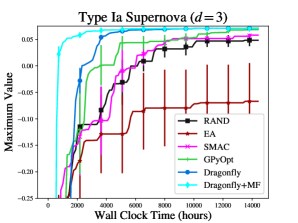
Type Ia Supernova: We use data on Type Ia supernova for maximum likelihood inference on $3$ cosmological parameters, the Hubble constant, the dark matter fraction, and the dark energy fraction. We use data from Davis et al. (2007), and the likelihood is computed using the method described in Shchigolev (2017). This requires a one dimensional numerical integration for each point in the dataset. We construct a $p=2$ dimensional multi-fidelity problem where we can choose data set size $N\in[50,192]$ and perform the integration on grids of size $G\in[10^{2},10^{6}]$ via the trapezoidal rule. As the cost function for fidelity selection, we used $\lambda(N,G)=NG$. Our goal is to maximise the average log likelihood at $z_{\bullet}=[192,10^{6}]$. Each method was given a budget of 4 hours on a 3.3 GHz Intel Xeon processor with 512GB memory. The results are given in Figure 9 where we plot the maximum average log likelihood (higher is better) against wall clock time. The plot includes the time taken by each method to determine the next point for evaluation. We do not compare Spearmint and HyperOpt as they do not provide an API for optimisation on a time budget.

6.3 Experiments on Model Selection Problems

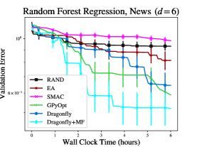
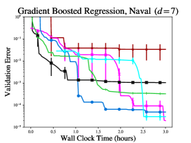
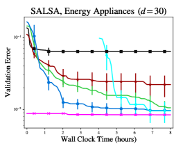
We begin with three experiments on tuning hyperparameters of regression methods, where we wish to find the hyperparameters with the smallest validation error. We set up a one dimensional fidelity space where a multi-fidelity algorithm may choose to use a subset of the dataset to approximate the performance when training with the entire training set. For multi-fidelity optimisation with Dragonfly, we use an exponential decay kernel for $\kappa_{\mathcal{Z}}$ (7). The results are presented in Figure 10, where we plot wall clock time against the validation error (lower is better). We do not compare Spearmint and HyperOpt since they do not provide an API for optimisation on a time budget.

Random forest regression, News popularity: In this experiment, we tune random forest regression (RFR) on the news popularity dataset (Fernandes et al., 2015). We tune 6 integral, discrete and Euclidean parameters available in the Scikit-Learn implementation of RFR. The training set had 20000 points, but could be approximated via a subset of size $z\in(5000,20000)$ by a multi-fidelity method. As the cost function, we use $\lambda(z)=z$, since training time is linear in the training set size. Each method was given a budget of 6 hours on a 3.3 GHz Intel Xeon processor with 512GB memory.

Figure 10: Results on the model selection problems in Section 6.3. The title states the method and data set used. In all figures, the $y$-axis is the validation error (lower is better), and the $x$-axis is wall clock time. All curves were produced by averaging over $10$ independent runs. Error bars indicate one standard error.

Dataset	Dragonfly	Dragonfly (lowest)	Dragonfly +MF	GPyOpt	SMAC	RAND	RAND (lowest)	Hyperband
RFR (News)	$0.6456$ $\pm 0.08044$	$.6631$ $\pm 0.0110$	$\bf 0.5203$ $\bf\pm 0.0805$	$0.5904$ $\pm 0.0635$	$0.9802$ $\pm 0.0291$	$0.9314$ $\pm 0.0371$	$0.8501$ $\pm 0.0563$	$0.6812$ $\pm 0.0412$
GBR (Naval)	$5.82\mathrm{e}{-5}$ $\pm$$1.52\mathrm{e}{-5}$	$\bf 1.14\mathrm{e}{-5}$ $\bf\pm$$\bf 7.3\mathrm{e}{-7}$	$3.00\mathrm{e}{-5}$ $\pm$$1.00\mathrm{e}{-5}$	$3.26\mathrm{e}{-4}$ $\pm$$1.46\mathrm{e}{-5}$	$1.97\mathrm{e}{-5}$ $\pm$$5.27\mathrm{e}{-6}$	$1.04\mathrm{e}{-3}$ $\pm$$1.10\mathrm{e}{-5}$	$1.31\mathrm{e}{-5}$ $\pm$$2.34\mathrm{e}{-6}$	$\bf 1.13\mathrm{e}{-5}$ $\bf\pm$$\bf 6.4\mathrm{e}{-7}$
SALSA (Energy)	$0.0097$ $\pm 0.0015$	$0.9950$ $\pm 0.0033$	$0.0095$ $\pm 0.0031$	$0.0105$ $\pm 0.0022$	$\bf 0.0084$ $\bf\pm 0.0003$	$0.0634$ $\pm 0.0019$	$0.9974$ $\pm 0.0032$	$0.3217$ $\pm 0.1032$

Table 2: Final least squared errors in the regression problems of Section 6.3. In addition to the methods in Figure 10, we also compare to Dragonfly and random search at the lowest fidelity, as well as Hyperband.

Gradient Boosted Regression, Naval Propulsion: In this experiment, we tune gradient boosted regression (GBR) on the naval propulsion dataset (Coraddu et al., 2016). We tune 7 integral, discrete and Euclidean parameters available in the Scikit-Learn implementation of GBR. The training set had 9000 points, but could be approximated via a subset of size $z\in(2000,9000)$ by a multi-fidelity method. As the cost function, we use $\lambda(z)=z$, since training time is linear in the training set size. Each method was given a budget of 3 hours on a 2.6 GHz Intel Xeon processor with 384GB memory.

SALSA, Energy Appliances: We use the SALSA regression method (Kandasamy and Yu, 2016) on the energy appliances dataset (Candanedo et al., 2017) to tune $30$ integral, discrete, and Euclidean parameters of the model. The training set had 8000 points, but could be approximated via a subset of size $z\in(2000,8000)$ by a multi-fidelity method. As the cost function, we use $\lambda(z)=z^{3}$, since training time is cubic in the training set size. Each method was given a budget of 8 hours on a 2.6 GHz Intel Xeon processor with 384GB memory. In this example, SMAC does very well because its (deterministically chosen) initial value luckily landed at a good configuration.

Table 2 compares the final error achieved by all methods on the above three datasets at the end of the respective optimisation budgets. In addition to the methods in Figure 10, we also show the results for BO (with Dragonfly) at the lowest fidelity, random search at the lowest fidelity and Hyperband (Li et al., 2018), which is a multi-fidelity method which uses random search and successive halving. For example, for BO and random search at the lowest fidelity on the RFR problem, we performed the same procedure as RAND and Dragonfly, but only using $5000$ points at each evaluation. Interestingly, we see that for the GBR experiment, BO using only a fraction of the training data, outperforms BO using the entire training set. This is because, in this problem, one can get good predictions even with $2000$ points, and the lower fidelity versions are able to do better since they are able to perform more evaluations within the specified time budget than the versions which query the higher fidelity.

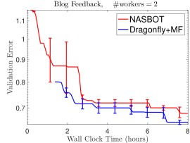
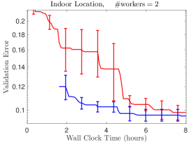
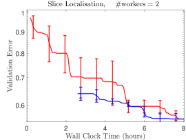
Experiments on Neural Architecture Search: Our next set of model selection experiments demonstrate the NAS features in Dragonfly. Here, we tune for the architecture of the network using the OTMANN kernel (Kandasamy et al., 2018b) and the learning rate. Each function evaluation, trains an architecture with stochastic gradient descent (SGD) with a fixed batch size of 256. We used the number of batch iterations in a one dimensional fidelity space, i.e. $\mathcal{Z}=[4000,20000]$ for Dragonfly while NASBOT always queried with $z_{\bullet}=20,000$ iterations. We test both methods in an asynchronously parallel set up of two GeForce GTX 970 (4GB) GPU workers with a computational budget of $8$ hours. Additionally, we also impose the following constraints on the space of architectures: maximum number of layers: $60$, maximum mass: $10^{8}$, maximum in/out degree: $5$, maximum number of edges: $200$, maximum number of units per layer: $1024$, minimum number of units per layer: $8$. We present the results of our experiments on the blog feedback (Buza, 2014), indoor location (Torres-Sospedra et al., 2014), and slice localisation (Graf et al., 2011), datasets in Figure 11. For reference, we also show the corresponding results for a vanilla implementation of NASBOT (Kandasamy et al., 2018b). Dragonfly outperforms NASBOT primarily because it is able to use cheaper evaluations to approximate fully trained models. Additionally, it benefits from tuning the learning rate and using robust techniques for selecting the acquisition and GP hyperparameters.

Figure 11: Results on the neural architecture search experiments. In all figures, the $x$-axis is wall clock time. The $y$ axis is the mean squared validation error (lower is better). In all cases, we used a parallel set up of two asynchronous workers, where each worker is a single GPU training a single model. We used a one dimensional fidelity space where we chose the number of batch iterations from 4000 to 20,000 ($z_{\bullet}=20,000$). All figures were averaged over 5 independent runs. Error bars indicate one standard error.

7 Conclusion

Bayesian optimisation is a powerful framework for optimising expensive blackbox functions. However, with increasingly expensive function evaluations and demands to optimise over complex input spaces, BO methods face new challenges today. In this work, we describe our multiple efforts to scale up BO to address the demands of modern large scale applications and techniques for improving robustness of BO methods. We implement them in an integrated fashion in an open source platform, Dragonfly, and demonstrate that they outperform existing platforms for BO in a variety of applications. Going forward, we wish to integrate techniques for multi-objective optimisation (Paria et al., 2018) and for using customised models via probabilistic programming (Neiswanger et al., 2019).

Acknowledgements:

This work was funded by DOE grant DESC0011114, NSF grant IIS1563887, and the DARPA D3M program. This work was done when KK was a Ph.D. student at Carnegie Mellon University, where he was supported by a Facebook fellowship and a Siebel scholarship. We thank Anthony Yu, Shuli Jiang, and Shalom Yiblet for assisting with the development of Dragonfly.

References

- Auer (2003) Peter Auer. Using Confidence Bounds for Exploitation-Exploration Trade-offs. Journal of Machine Learning Research, 2003.
- Authors (2016) TG Authors. GPyOpt: A Bayesian Optimization Framework in Python, 2016.
- Bergstra et al. (2013) James Bergstra, Dan Yamins, and David D Cox. Hyperopt: A Python Library for Optimizing the Hyperparameters of Machine Learning Algorithms. In 12th Python in Science Conference, 2013.
- Buza (2014) Krisztian Buza. Feedback Prediction for Blogs. In Data Analysis, Machine Learning and Knowledge Discovery. 2014.
- Candanedo et al. (2017) Luis M Candanedo, Véronique Feldheim, and Dominique Deramaix. Data Driven Prediction Models of Energy Use of Appliances in a Low-energy House. Energy and Buildings, 2017.
- Chen et al. (2012) Bo Chen, Rui Castro, and Andreas Krause. Joint Optimization and Variable Selection of High-dimensional Gaussian Processes. In International Conference on Machine Learning, 2012.
- Coraddu et al. (2016) Andrea Coraddu, Luca Oneto, Aessandro Ghio, Stefano Savio, Davide Anguita, and Massimo Figari. Machine Learning Approaches for Improving Condition-based Maintenance of Naval Propulsion Plants. Journal of Engineering for the Maritime Environment, 2016.
- Davis et al. (2007) Tamara M Davis, Edvard Mörtsell, Jesper Sollerman, Andrew C Becker, Stephanie Blondin, P Challis, Alejandro Clocchiatti, AV Filippenko, RJ Foley, Peter M Garnavich, et al. Scrutinizing Exotic Cosmological Models Using ESSENCE Supernova Data Combined with Other Cosmological Probes. The Astrophysical Journal, 2007.
- Desautels et al. (2014) Thomas Desautels, Andreas Krause, and Joel W Burdick. Parallelizing Exploration-Exploitation Tradeoffs in Gaussian Process Bandit Optimization. Journal of Machine Learning Research, 2014.
- Djolonga et al. (2013) Josip Djolonga, Andreas Krause, and Volkan Cevher. High-Dimensional Gaussian Process Bandits. In Advances in Neural Information Processing Systems, 2013.
- Duvenaud et al. (2011) David K. Duvenaud, Hannes Nickisch, and Carl Edward Rasmussen. Additive Gaussian Processes. In Neural Information Processing Systems, 2011.
- Fernandes et al. (2015) Kelwin Fernandes, Pedro Vinagre, and Paulo Cortez. A Proactive Intelligent Decision Support System for Predicting the Popularity of Online News. In Portuguese Conference on Artificial Intelligence, 2015.
- Frazier et al. (2009) Peter Frazier, Warren Powell, and Savas Dayanik. The Knowledge-Gradient Policy for Correlated Normal Beliefs. INFORMS Journal on Computing, 21, 2009.
- Gardner et al. (2017) Jacob Gardner, Chuan Guo, Kilian Weinberger, Roman Garnett, and Roger Grosse. Discovering and Exploiting Additive Structure for Bayesian Optimization. In Artificial Intelligence and Statistics, 2017.
- Ginsbourger et al. (2011) David Ginsbourger, Janis Janusevskis, and Rodolphe Le Riche. Dealing with Asynchronicity in Parallel Gaussian Process Based Global Optimization. In Conference of the ERCIM WG on Computing and Statistics, 2011.
- Gonzalez et al. (2014) Javier Gonzalez, Joseph Longworth, David James, and Neil Lawrence. Bayesian Optimization for Synthetic Gene Design. In NIPS Workshop on Bayesian Optimization, 2014.
- González et al. (2016) Javier González, Zhenwen Dai, Philipp Hennig, and Neil Lawrence. Batch Bayesian Optimization via Local Penalization. In Artificial Intelligence and Statistics, 2016.
- Graf et al. (2011) Franz Graf, Hans-Peter Kriegel, Matthias Schubert, Sebastian Pölsterl, and Alexander Cavallaro. 2D Image Registration in CT Images Using Radial Image Descriptors. In Medical Imaging and Computer-Assisted Intervention, 2011.
- Griffiths and Hernández-Lobato (2020) Ryan-Rhys Griffiths and José Miguel Hernández-Lobato. Constrained Bayesian Optimization for Automatic Chemical Design using Variational Autoencoders. Chemical Science, 2020.
- Grill et al. (2015) Jean-Bastien Grill, Michal Valko, and Rémi Munos. Black-box Optimization of Noisy Functions with Unknown Smoothness. In Neural Information Processing Systems, 2015.
- Györfi et al. (2002) László Györfi, Micael Kohler, Adam Krzyzak, and Harro Walk. A Distribution Free Theory of Nonparametric Regression. Springer Series in Statistics, 2002.
- He et al. (2016) Kaiming He, Xiangyu Zhang, Shaoqing Ren, and Jian Sun. Deep Residual Learning for Image Recognition. In IEEE Conference on Computer Vision and Pattern Recognition, 2016.
- Hennig and Schuler (2012) Philipp Hennig and Christian J. Schuler. Entropy Search for Information-efficient Global Optimization. Journal of Machine Learning Research, pages 1809–1837, 2012.
- Hoffman et al. (2011) Matthew Hoffman, Eric Brochu, and Nando de Freitas. Portfolio Allocation for Bayesian Optimization. In Conference on Uncertainty in Artificial Intelligence, 2011.
- Hoffman and Shahriari (2014) Matthew W Hoffman and Bobak Shahriari. Modular Mechanisms for Bayesian Optimization. In NIPS Workshop on Bayesian Optimization, 2014.
- Hornby et al. (2006) Gregory Hornby, Al Globus, Derek Linden, and Jason Lohn. Automated Antenna Design with Evolutionary Algorithms. In Space 2006. 2006.
- Huang et al. (2006) Deng Huang, Theodore T Allen, William I Notz, and R Allen Miller. Sequential Kriging Optimization Using Multiple-fidelity Evaluations. Structural and Multidisciplinary Optimization, 2006.
- Huang et al. (2017) Gao Huang, Zhuang Liu, Kilian Q Weinberger, and Laurens van der Maaten. Densely Connected Convolutional Networks. In Proceedings of the IEEE Conference on Computer Vision and Pattern Recognition, 2017.
- Hutter et al. (2011) Frank Hutter, Holger H. Hoos, and Kevin Leyton-Brown. Sequential Model-based Optimization for General Algorithm Configuration. In Learning and Intelligent Optimization, 2011. URL https://automl.github.io/SMAC3/master/.
- Jenatton et al. (2017) Rodolphe Jenatton, Cedric Archambeau, Javier González, and Matthias Seeger. Bayesian Optimization with Tree-structured Dependencies. In International Conference on Machine Learning, 2017.
- Jones et al. (1993) Donald R Jones, Cary D Perttunen, and Bruce E Stuckman. Lipschitzian Optimization Without the Lipschitz Constant. Journal of Optimization Theory and Applications, 1993.
- Jones et al. (1998) Donald R. Jones, Matthias Schonlau, and William J. Welch. Efficient Global Optimization of Expensive Black-Box Functions. Journal of Global Optimization, 1998.
- Kandasamy and Yu (2016) Kirthevasan Kandasamy and Yaoliang Yu. Additive Approximations in High Dimensional Nonparametric Regression via the SALSA. In International Conference on Machine Learning, 2016.
- Kandasamy et al. (2015a) Kirthevasan Kandasamy, Jeff Schenider, and Barnabás Póczos. High Dimensional Bayesian Optimisation and Bandits via Additive Models. In International Conference on Machine Learning, 2015a.
- Kandasamy et al. (2015b) Kirthevasan Kandasamy, Jeff Schneider, and Barnabás Póczos. Bayesian Active Learning for Posterior Estimation. In International Joint Conference on Artificial Intelligence, 2015b.
- Kandasamy et al. (2016a) Kirthevasan Kandasamy, Gautam Dasarathy, Junier Oliva, Jeff Schenider, and Barnabás Póczos. Gaussian Process Bandit Optimisation with Multi-fidelity Evaluations. In Advances in Neural Information Processing Systems, 2016a.
- Kandasamy et al. (2016b) Kirthevasan Kandasamy, Gautam Dasarathy, Junier B Oliva, Jeff Schneider, and Barnabas Poczos. Multi-fidelity Gaussian Process Bandit Optimisation. arXiv preprint arXiv:1603.06288, 2016b.
- Kandasamy et al. (2016c) Kirthevasan Kandasamy, Gautam Dasarathy, Jeff Schneider, and Barnabas Poczos. The Multi-fidelity Multi-armed Bandit. In Advances in Neural Information Processing Systems, 2016c.
- Kandasamy et al. (2017) Kirthevasan Kandasamy, Gautam Dasarathy, Jeff Schneider, and Barnabás Póczos. Multi-fidelity Bayesian Optimisation with Continuous Approximations. In International Conference on Machine Learning, 2017.
- Kandasamy et al. (2018a) Kirthevasan Kandasamy, Akshay Krishnamurthy, Jeff Schneider, and Barnabás Póczos. Parallelised Bayesian Optimisation via Thompson Sampling. In International Conference on Artificial Intelligence and Statistics, 2018a.
- Kandasamy et al. (2018b) Kirthevasan Kandasamy, Willie Neiswanger, Jeff Schneider, Barnabas Poczos, and Eric Xing. Neural Architecture Search with Bayesian Optimisation and Optimal Transport. In Advances in Neural Information Processing Systems, 2018b.
- Klein et al. (2015) Aaron Klein, Simon Bartels, Stefan Falkner, Philipp Hennig, and Frank Hutter. Towards Efficient Bayesian Optimization for Big Data. In NIPS 2015 Bayesian Optimization Workshop, 2015.
- Kushner (1964) Harold J Kushner. A New Method of Locating the Maximum Point of An Arbitrary Multipeak Curve in the Presence of Noise. Journal of Basic Engineering, 1964.
- Li et al. (2016) Chun-Liang Li, Kirthevasan Kandasamy, Barnabás Póczos, and Jeff Schneider. High Dimensional Bayesian Optimization via Restricted Projection Pursuit Models. In Artificial Intelligence and Statistics, 2016.
- Li and Talwalkar (2019) Liam Li and Ameet Talwalkar. Random Search and Reproducibility for Neural Architecture Search. arXiv preprint arXiv:1902.07638, 2019.
- Li et al. (2018) Lisha Li, Kevin Jamieson, Giulia DeSalvo, Afshin Rostamizadeh, and Ameet Talwalkar. Hyperband: A Novel Bandit-Based Approach to Hyperparameter Optimization. Journal of Machine Learning Research, 2018.
- Liu et al. (2017) Hanxiao Liu, Karen Simonyan, Oriol Vinyals, Chrisantha Fernando, and Koray Kavukcuoglu. Hierarchical representations for efficient architecture search. arXiv preprint arXiv:1711.00436, 2017.
- Liu et al. (2019) Hanxiao Liu, Karen Simonyan, and Yiming Yang. DARTS: Differentiable Architecture Search. In International Conference on Learning Representations, 2019.
- Malkomes et al. (2016) Gustavo Malkomes, Charles Schaff, and Roman Garnett. Bayesian Optimization for Automated Model Selection. In Neural Information Processing Systems, 2016.
- Mendoza et al. (2016) Hector Mendoza, Aaron Klein, Matthias Feurer, Jost Tobias Springenberg, and Frank Hutter. Towards Automatically-tuned Neural Networks. In Workshop on Automatic Machine Learning, 2016.
- Neal (2003) Radford M Neal. Slice Sampling. Annals of statistics, 2003.
- Neiswanger et al. (2019) Willie Neiswanger, Kirthevasan Kandasamy, Barnabas Poczos, Jeff Schneider, and Eric Xing. ProBO: a Framework for Using Probabilistic Programming in Bayesian Optimization. arXiv preprint arXiv:1901.11515, 2019.
- Paria et al. (2018) Biswajit Paria, Kirthevasan Kandasamy, and Barnabás Póczos. A Flexible Multi-Objective Bayesian Optimization Approach using Random Scalarizations. arXiv preprint arXiv:1805.12168, 2018.
- Parkinson et al. (2006) David Parkinson, Pia Mukherjee, and Andrew R Liddle. A Bayesian Model Selection Analysis of WMAP3. Physical Review, 2006.
- Poloczek et al. (2017) Matthias Poloczek, Jialei Wang, and Peter Frazier. Multi-Information Source Optimization. In Advances in Neural Information Processing Systems, 2017.
- Qin et al. (2017) Chao Qin, Diego Klabjan, and Daniel Russo. Improving the Expected Improvement Algorithm. In Advances in Neural Information Processing Systems, 2017.
- Rasmussen and Williams (2006) Carl Edward Rasmussen and Christopher KI Williams. Gaussian Processes for Machine Learning. Adaptative Computation and Machine Learning Series. University Press Group Limited, 2006.
- Rolland et al. (2018) Paul Rolland, Jonathan Scarlett, Ilija Bogunovic, and Volkan Cevher. High-Dimensional Bayesian Optimization via Additive Models with Overlapping Groups. In International Conference on Artificial Intelligence and Statistics, 2018.
- Sen et al. (2018a) Rajat Sen, Kirthevasan Kandasamy, and Sanjay Shakkottai. Multi-Fidelity Black-Box Optimization with Hierarchical Partitions. In International Conference on Machine Learning, 2018a.
- Sen et al. (2018b) Rajat Sen, Kirthevasan Kandasamy, and Sanjay Shakkottai. Noisy Blackbox Optimization with Multi-Fidelity Queries: A Tree Search Approach. arXiv preprint arXiv:1810.10482, 2018b.
- Shah and Ghahramani (2015) Amar Shah and Zoubin Ghahramani. Parallel Predictive Entropy Search for Batch Global Optimization of Expensive Objective Functions. In Advances in Neural Information Processing Systems, 2015.
- Shahriari et al. (2014) Bobak Shahriari, Ziyu Wang, Matthew W Hoffman, Alexandre Bouchard-Côté, and Nando de Freitas. An Entropy Search Portfolio for Bayesian Optimization. arXiv preprint arXiv:1406.4625, 2014.
- Shchigolev (2017) VK Shchigolev. Calculating Luminosity Distance Versus Redshift in FLRW Cosmology via Homotopy Perturbation Method. Gravitation and Cosmology, 2017.
- Snoek et al. (2012) Jasper Snoek, Hugo Larochelle, and Ryan P Adams. Practical Bayesian Optimization of Machine Learning Algorithms. In Neural Information Processing Systems, 2012.
- Snoek et al. (2015) Jasper Snoek, Oren Rippel, Kevin Swersky, Ryan Kiros, Nadathur Satish, Narayanan Sundaram, Mostofa Patwary, Mr Prabhat, and Ryan Adams. Scalable Bayesian Optimization using Deep Neural Networks. In International Conference on Machine Learning, 2015.
- Song et al. (2019) Jialin Song, Yuxin Chen, and Yisong Yue. A General Framework for Multi-fidelity Bayesian Optimization with Gaussian Processes. 2019.
- Springenberg et al. (2016) Jost Tobias Springenberg, Aaron Klein, Stefan Falkner, and Frank Hutter. Bayesian Optimization with Robust Bayesian Neural Networks. In Advances in Neural Information Processing Systems 29, December 2016.
- Srinivas et al. (2010) Niranjan Srinivas, Andreas Krause, Sham Kakade, and Matthias Seeger. Gaussian Process Optimization in the Bandit Setting: No Regret and Experimental Design. In International Conference on Machine Learning, 2010.
- Swersky et al. (2013) Kevin Swersky, Jasper Snoek, and Ryan P Adams. Multi-task Bayesian Optimization. In Neural Information Processing Systems, 2013.
- Swersky et al. (2014a) Kevin Swersky, David Duvenaud, Jasper Snoek, Frank Hutter, and Michael A Osborne. Raiders of the Lost Architecture: Kernels for Bayesian Optimization in Conditional Parameter Spaces. arXiv preprint arXiv:1409.4011, 2014a.
- Swersky et al. (2014b) Kevin Swersky, Jasper Snoek, and Ryan Prescott Adams. Freeze-thaw Bayesian Optimization. arXiv preprint arXiv:1406.3896, 2014b.
- Tegmark et al. (2006) Max Tegmark, Daniel J Eisenstein, Michael A Strauss, David H Weinberg, Michael R Blanton, Joshua A Frieman, Masataka Fukugita, James E Gunn, Andrew JS Hamilton, Gillian R Knapp, et al. Cosmological Constraints from the SDSS Luminous Red Galaxies. Physical Review, 2006.
- Thompson (1933) William R Thompson. On the Likelihood that one Unknown Probability Exceeds Another in View of the Evidence of Two Samples. Biometrika, 1933.
- Torres-Sospedra et al. (2014) Joaquín Torres-Sospedra, Raúl Montoliu, Adolfo Martínez-Usó, Joan P Avariento, Tomás J Arnau, Mauri Benedito-Bordonau, and Joaquín Huerta. UJIIndoorLoc: A New Multi-building and Multi-floor Database for WLAN Fingerprint-based Indoor Localization Problems. In Indoor Positioning and Indoor Navigation, 2014, 2014.
- Villani (2003) Cédric Villani. Topics in Optimal Transportation. American Mathematical Soc., 2003.
- Wang et al. (2017) Zi Wang, Chengtao Li, Stefanie Jegelka, and Pushmeet Kohli. Batched High-dimensional Bayesian Optimization via Structural Kernel Learning. In International Conference on Machine Learning-Volume 70, 2017.
- Wang et al. (2018) Zi Wang, Clement Gehring, Pushmeet Kohli, and Stefanie Jegelka. Batched Large-scale Bayesian Optimization in High-dimensional Spaces. In International Conference on Artificial Intelligence and Statistics, pages 745–754, 2018.
- Wang et al. (2013) Ziyu Wang, Masrour Zoghi, Frank Hutter, David Matheson, and Nando de Freitas. Bayesian Optimization in High Dimensions via Random Embeddings. In International Joint Conference on Artificial Intelligence, 2013.
- Yamins et al. (2013) Daniel Yamins, David Tax, and James S. Bergstra. Making a Science of Model Search: Hyperparameter Optimization in Hundreds of Dimensions for Vision Architectures. In International Conference on Machine Learning, 2013.
- Zhang and Chaudhuri (2015) Chicheng. Zhang and Kamalika. Chaudhuri. Active Learning from Weak and Strong Labelers. In Neural Information Processing Systems, 2015.
- Zoph and Le (2017) Barret Zoph and Quoc V Le. Neural Architecture Search with Reinforcement Learning. In International Conference on Learning Representations, 2017.