On confidence intervals centered on bootstrap smoothed estimators

Paul Kabailaβˆ— and Christeen Wijethunga

Department of Mathematics and Statistics, La Trobe University, Australia

ABSTRACT

Bootstrap smoothed (bagged) estimators have been proposed as an improvement on estimators found after preliminary data-based model selection. Efron, 2014, derived a widely applicable formula for a delta method approximation to the standard deviation of the bootstrap smoothed estimator. He also considered a confidence interval centered on the bootstrap smoothed estimator, with width proportional to the estimate of this standard deviation. Kabaila and Wijethunga, 2019, assessed the performance of this confidence interval in the scenario of two nested linear regression models, the full model and a simpler model, for the case of known error variance and preliminary model selection using a hypothesis test. They found that the performance of this confidence interval was not substantially better than the usual confidence interval based on the full model, with the same minimum coverage. We extend this assessment to the case of unknown error variance by deriving a computationally convenient exact formula for the ideal (i.e. in the limit as the number of bootstrap replications diverges to infinity) delta method approximation to the standard deviation of the bootstrap smoothed estimator. Our results show that, unlike the known error variance case, there are circumstances in which this confidence interval has attractive properties.

Keywords: Bootstrap smoothed estimator, coverage probability, confidence interval, expected length, model selection

1. Introduction

In applied statistics there is usually some uncertainty as to which explanatory variables should be included in the model. The first attempt to deal with this β€˜model uncertainty’ was to use preliminary data-based model selection employing either hypothesis tests or minimizing a criterion such as the Akaike Information Criterion (Akaike, 1974). This model selection was followed by the statistical inference of interest, based on the assumption that the selected model had been given to us a priori, as the true model. This assumption is false and typically leads to incorrect and misleading inference (see e.g. Kabaila, 2009 and Leeb and PΓΆtscher, 2005).

Bootstrap smoothed (or bagged; Breiman, 1996) estimators have been proposed as an improvement on estimators found after preliminary data-based model selection (post-model-selection estimators). Bootstrap smoothed estimators are smoothed versions of the post-model-selection estimator. The key result of Efron (2014) is a formula for a delta method approximation, ${\bf sd}_{\rm delta}$, to the standard deviation of the bootstrap smoothed estimator. This formula is valid for any exponential family of models and has the attractive feature that it simply re-uses the parametric bootstrap replications that were employed to find this estimator. It also has the attractive feature that it is applicable in the context of complicated data-based model selection. Kabaila and Wijethunga (2019) consider a confidence interval (CI) centered on the bootstrap smoothed estimator, with nominal coverage $1-\alpha$, and half-width equal to the $1-\alpha/2$ quantile of the standard normal distribution multiplied by the estimate of ${\bf sd}_{\rm delta}\,$. We call this interval the ${\bf sd}_{\rm delta}\,{\bf interval}$.

This CI has similarities with the frequentist model averaged CIs proposed by Buckland etΒ al. (1997), Fletcher and Turek (2011) and Turek and Fletcher (2012). All of these CIs need to have their performances, in terms of coverage probability and expected length, carefully assessed before they can be recommended for general use by applied statisticians. We believe that such assessments are best carried out through a sequence of increasingly complicated β€˜test scenarios’.

The simplest test scenario consists of two nested linear regression models, where the simpler model is given by a specified linear combination of the regression parameters being set to zero. In this test scenario, the scalar parameter of interest is a distinct linear combination of the regression parameters and we assume independent and identically distributed normal errors, with error variance assumed known. Kabaila and Wijethunga (2019) provide a detailed assessment of the performance of the ${\bf sd}_{\rm delta}\,{\bf interval}$ in this test scenario if the simpler model is selected when a preliminary hypothesis test accepts the null hypothesis that this simpler model is correct. They found that, while this CI performed much better than the post-model-selection confidence interval in terms of minimum coverage probability, its performance in terms of expected length was not substantially better than the usual CI based on the full model, with the same minimum coverage.

The next simplest test scenario is the same, but with unknown error variance. Kabaila etΒ al. (2016) and Kabaila etΒ al. (2017) used this test scenario to provide a detailed assessment of the performance of the CIs proposed by Fletcher and Turek (2011) and Turek and Fletcher (2012). Our aim is to extend the assessment made by Kabaila and Wijethunga (2019) of the performance of the ${\bf sd}_{\rm delta}\,{\bf interval}$ to this test scenario.

We apply Theorem 2 of Efron (2014) to derive a computationally convenient exact formula for the ideal (i.e. in the limit as the number of bootstrap replications diverges to infinity) delta method approximation to the standard deviation of the bootstrap smoothed estimator. An outline of this derivation, which is quite complicated, is provided in Appendix A.1. Our computed results show that, unlike the case that the error variance is assumed known, there are circumstances in which the expected length properties of the ${\bf sd}_{\rm delta}\,{\bf interval}$ are quite attractive.

2. The two nested regression models and the post-model-selection estimator

We consider two nested linear regression models: the full model ${\cal M}_{2}$ and the simpler model ${\cal M}_{1}$. Suppose that the full model ${\cal M}_{2}$ is given by

$$\mbox{$\bm{y}$}=\bm{X}\bm{\beta}+\bm{\varepsilon}$$

where $\bm{y}$ is a random $n$-vector of responses, $\bm{X}$ is a known $n\times p$ matrix with linearly independent columns ($p<n$), $\bm{\beta}$ is an unknown $p$-vector of parameters and $\bm{\varepsilon}\sim N(\bm{0},\sigma^{2}\bm{I})$, with $\sigma^{2}$ an unknown positive parameter. Suppose that $\bm{\beta}=[\theta,\tau,\bm{\lambda}^{\top}]^{\top}$, where $\theta$ is the scalar parameter of interest, $\tau$ is a scalar parameter used in specifying the model ${\cal M}_{1}$ and $\bm{\lambda}$ is a ($p-2$)-dimensional parameter vector. The model ${\cal M}_{1}$ is ${\cal M}_{2}$ with $\tau=0$. As shown in Appendix A of Kabaila and Wijethunga (2019), this scenario can be obtained by a change of parametrization from a more general scenario. Let $m=n-p$.

Let $\widehat{\bm{\beta}}$ denote the least squares estimator of $\bm{\beta}$, so that $\widehat{\bm{\beta}}=(\bm{X}^{\top}\bm{X})^{-1}\bm{X}^{\top}\mbox{$\bm{y}$}$, and $\widehat{\sigma}^{2}=(\mbox{$\bm{y}$}-\bm{X}\widehat{\bm{\beta}})^{\top}(\mbox{$\bm{y}$}-\bm{X}\widehat{\bm{\beta}})/m$. Also let $\widehat{\theta}$ and $\widehat{\tau}$ denote the first and second components of $\widehat{\bm{\beta}}$, respectively. Now let $v_{\theta}=\mbox{$\textrm{{var}}$}(\widehat{\theta})/\sigma^{2}$, $v_{\tau}=\mbox{$\textrm{{var}}$}(\widehat{\tau})/\sigma^{2}$ and $\rho=\mbox{$\textrm{{corr}}$}(\widehat{\theta},\widehat{\tau})=v_{\theta\tau}/(v_{\theta}v_{\tau})^{1/2}$, where $v_{\theta\tau}=\mbox{$\textrm{{cov}}$}(\widehat{\theta},\widehat{\tau})/\sigma^{2}$. Note that $v_{\theta}$, $v_{\tau}$, $v_{\theta\tau}$ and $\rho$ are known. Let $\gamma=\tau/\big{(}\sigma v_{\tau}^{1/2}\big{)}$, which is an unknown parameter, and $\widehat{\gamma}=\widehat{\tau}/(\widehat{\sigma}{v_{\tau}}^{1/2})$.

Suppose that we carry out a preliminary test of the null hypothesis $\tau=0$ against the alternative hypothesis Ο„β‰ 0𝜏0\tau\neq 0 and that we choose the model ${\cal M}_{1}$ if this null hypothesis is accepted; otherwise we choose the model ${\cal M}_{2}$. Let $t_{m}(a)$ be defined by $P(T\leq t_{m}(a))=1-a/2$ for $T\sim t_{m}$. Suppose that we accept the null hypothesis when $|\widehat{\gamma}|\leq t_{m}(\widetilde{\alpha})$; otherwise we reject the null hypothesis. The size of this preliminary test is $\widetilde{\alpha}$. Therefore the post-model-selection estimator of $\theta$ is equal to

$$\widehat{\theta}_{\textsc{\tiny PMS}}=\begin{cases}\widehat{\theta}-\displaystyle{\frac{v_{\theta\tau}}{v_{\tau}}}\widehat{\tau}\qquad\text{\ \ \ \ if }\ |\widehat{\gamma}|\leq t_{m}(\widetilde{\alpha})\\ \widehat{\theta}\qquad\text{\ \ \ \ otherwise}.\end{cases}$$

Henceforth, suppose that $1-\alpha$ and $\widetilde{\alpha}$ are given.

3. Computationally convenient exact formulas for the ideal bootstrap smoothed estimate and the delta method approximation to its standard deviation

The parametric bootstrap smoothed estimate of $\theta$ is obtained as follows. Note that $\widehat{\bm{\beta}}\sim N\big{(}\bm{\beta},\sigma^{2}(\bm{X}^{\top}\bm{X})^{-1}\big{)}$ and, independently, $m^{1/2}\widehat{\sigma}/\sigma\sim\chi_{m}$ (if $Q\sim\chi_{m}^{2}$ then $Q^{1/2}$ is said to have a $\chi_{m}$ distribution). To make the dependence of $\widehat{\theta}_{\textsc{\tiny PMS}}$ on $(\widehat{\bm{\beta}},\widehat{\sigma})$ explicit, write $\widehat{\theta}_{\textsc{\tiny PMS}}=g(\widehat{\bm{\beta}},\widehat{\sigma})$. For the estimate $(\widehat{\bm{\beta}},\widehat{\sigma})$ treated as the true parameter value, suppose that $\widehat{\bm{\beta}}^{*}\sim N\big{(}\widehat{\bm{\beta}},\widehat{\sigma}^{2}(\bm{X}^{\top}\bm{X})^{-1}\big{)}$ and, independently, $m^{1/2}\widehat{\sigma}^{*}/\widehat{\sigma}\sim\chi_{m}$. A parametric bootstrap sample of size $B$ consists of independent observations $\big{(}\widehat{\bm{\beta}}_{1}^{*},\widehat{\sigma}_{1}^{*}\big{)},\big{(}\widehat{\bm{\beta}}_{2}^{*},\widehat{\sigma}_{2}^{*}\big{)},\dots,\big{(}\widehat{\bm{\beta}}_{B}^{*},\widehat{\sigma}_{B}^{*}\big{)},$ of the random vector $\big{(}\widehat{\bm{\beta}}^{*},\widehat{\sigma}^{*}\big{)}$. The parametric smoothed estimate of $\theta$ is defined to be

$$\frac{1}{B}\sum_{i=1}^{B}g\big{(}\widehat{\bm{\beta}}_{i}^{*},\widehat{\sigma}_{i}^{*}\big{)}.$$

The limit as the number of boostrap replications $B\rightarrow\infty$ of this quantity is called by Efron (2014) the ideal bootstrap smoothed estimate of $\theta$. We denote this ideal boostrap smoothed estimate by $\widetilde{\theta}$ and observe that it may be obtained as follows. Let $E_{\bm{\beta},\sigma}(\widehat{\theta}_{\textsc{\tiny PMS}})$ denote the expected value of $\widehat{\theta}_{\textsc{\tiny PMS}}$, for true parameter value $(\bm{\beta},\sigma)$. The ideal bootstrap smoothed estimate $\widetilde{\theta}$ is obtained by first evaluating $E_{\bm{\beta},\sigma}(\widehat{\theta}_{\textsc{\tiny PMS}})$ and then replacing $(\bm{\beta},\sigma)$ by $\big{(}\widehat{\bm{\beta}},\widehat{\sigma}\big{)}$.

Let $W=\widehat{\sigma}/\sigma$ and define $k_{m}(\gamma)$ to be

$$\int_{0}^{\infty}\Big{(}\phi(d_{m}w+\gamma)-\phi(d_{m}w-\gamma)+\gamma\big{(}\Phi(d_{m}w-\gamma)-\Phi(-d_{m}w-\gamma)\big{)}\Big{)}\,f_{W}(w)\,dw,$$ (1)

where $\phi$ and $\Phi$ denote the $N(0,1)$ pdf and cdf, respectively, $d_{m}=t_{m}(\widetilde{\alpha})$ and $f_{W}$ denotes the probability density function of $W$. As proved in Appendix B of Kabaila and Wijethunga (2019), $E_{\bm{\beta},\sigma}(\widehat{\theta}_{\textsc{\tiny PMS}})=\theta-\rho\,\sigma\,v_{\theta}^{1/2}\,k_{m}(\gamma)$. Therefore

$$\widetilde{\theta}=\widehat{\theta}-\rho\,\widehat{\sigma}\,v_{\theta}^{1/2}\,k_{m}(\widehat{\gamma}).$$

An outline of the proof of the following new theorem is given in Appendix A.1.

Theorem 1.

An application of Theorem 2 of Efron (2014) leads to the ideal (i.e. in the limit as the number of boostrap replications $B\rightarrow\infty$) delta method approximation to the standard deviation of $\widetilde{\theta}$, denoted by ${\bf sd}_{\rm delta}(\gamma,\sigma)$, which is $\sigma v_{\theta}^{1/2}\,r_{\,\rm delta}(\gamma)$, where

$$r_{\,\rm delta}(\gamma)=\Bigg{(}\frac{\rho^{2}}{2n}\Big{(}k_{m}(\gamma)+h_{m}(\gamma)-\gamma\,q_{m}(\gamma)\Big{)}^{2}+1-2\rho^{2}q_{m}(\gamma)+\rho^{2}q_{m}^{2}(\gamma)\Bigg{)}^{1/2}.$$ (2)

Here $q_{m}(\gamma)$ is defined to be

$$\int_{0}^{\infty}\big{(}-d_{m}w\,\phi(d_{m}w+\gamma)-d_{m}w\,\phi(d_{m}w-\gamma)+\Phi(d_{m}w-\gamma)-\Phi(-d_{m}w-\gamma)\big{)}\,f_{W}(w)\,dw$$ (3)

and

$$h_{m}(\gamma)=\int_{0}^{\infty}\Big{(}(d_{m}w)^{2}\phi(d_{m}w+\gamma)-(d_{m}w)^{2}\phi(d_{m}w-\gamma)\Big{)}\,f_{W}(w)\,dw,$$ (4)

where, as before, $d_{m}=t_{m}(\widetilde{\alpha})$.

We expect, intuitively, that the results obtained for the case that $\sigma^{2}$ is unknown (so that it must be estimated from the data) and $m\rightarrow\infty$ should be the same as for the case that $\sigma^{2}$ is known. Suppose that $p$ is fixed and $n\rightarrow\infty$, so that $m=n-p$ also diverges to $\infty$. As expected, the ideal delta method approximation to the standard deviation of $\widetilde{\theta}$ given by Theorem 1 converges to the corresponding quantity given by Theorem 2 of Kabaila and Wijethunga (2019), which deals with the case that $\sigma^{2}$ is known.

4. Computationally convenient exact formula for the coverage probability of the confidence interval centered on the bootstrap smoothed estimator

Consider the CI for $\theta$ centered on the bootstrap smoothed estimator $\widetilde{\theta}$, with nominal coverage $1-\alpha$,

$\displaystyle J_{\rm delta}$ $\displaystyle=\Big{[}\widetilde{\theta}-t_{m}(\alpha)\,{\bf sd}_{\rm delta}(\widehat{\gamma},\widehat{\sigma}),\,\widetilde{\theta}+t_{m}(\alpha)\,{\bf sd}_{\rm delta}(\widehat{\gamma},\widehat{\sigma})\Big{]}$
$\displaystyle=\Big{[}\widetilde{\theta}-t_{m}(\alpha)\,\widehat{\sigma}\,v_{\theta}^{1/2}\,r_{\,\rm delta}(\widehat{\gamma}),\,\widetilde{\theta}+t_{m}(\alpha)\,\widehat{\sigma}\,v_{\theta}^{1/2}\,r_{\,\rm delta}(\widehat{\gamma})\Big{]},$

which we call the ${\bf sd}_{\rm delta}$ interval. Note that when $\rho=0$, this CI is identical to the usual CI, with actual coverage $1-\alpha$, based on the full model ${\cal M}_{2}$. It may be shown that the coverage probability $P(\theta\in J_{\rm delta})$ is a function of $(\gamma,\rho)$. We therefore denote this coverage probability by ${\rm CP}_{\rm delta}(\gamma,\rho)$. The following theorem is proved in Appendix A.2.

Theorem 2.

Let

$\displaystyle\ell(h,w,\rho)$ $\displaystyle=-w\,t_{m}(\alpha)\,r_{\rm delta}\left(\frac{h}{w}\right)+w\,\rho\,\,k_{m}\left(\frac{h}{w}\right)$ (5)
$\displaystyle u(h,w,\rho)$ $\displaystyle=w\,t_{m}(\alpha)\,r_{\rm delta}\left(\frac{h}{w}\right)+w\,\rho\,\,k_{m}\left(\frac{h}{w}\right).$ (6)

Then ${\rm CP}_{\rm delta}(\gamma,\rho)$ is given by

$$\int_{0}^{\infty}\int_{-\infty}^{\infty}\Psi\Big{(}\ell(y+\gamma,w,\rho),u(y+\gamma,w,\rho);\rho(y),1-\rho^{2}\Big{)}\phi(y)\,dy\,f_{W}(w)\,dw,$$

where $\Psi\big{(}\ell,u;\mu,v\big{)}=P\big{(}\ell\leq Z\leq u\big{)}$ for $Z\sim N(\mu,v)$.

The expression (2) suggests that, for all sufficiently large $n$, ${\rm CP}_{\rm delta}(\gamma,\rho)$ is determined by $m$, for any given $(\gamma,\rho)$. Computational results for $n=25$ (described later in this section) and $n=100$ (not described either here or in the Supporting Material) suggest that, for all $n\geq 25$, ${\rm CP}_{\rm delta}(\gamma,\rho)$ is, for practical purposes, determined by $m$, for any given $(\gamma,\rho)$. It may be shown that ${\rm CP}_{\rm delta}(\gamma,\rho)$ is (a) an even function of $\gamma$ for each $\rho$ and (b) an even function of $\rho$ for each $\gamma$. It follows that, for given $n$ and $m$, we are able to encapsulate the coverage probability of the ${\bf sd}_{\rm delta}\,{\bf interval}$, for all possible choices of design matrix, parameter of interest $\theta$ and parameter $\tau$ that specifies the simpler model, using only the parameters $|\rho|$ and $|\gamma|$.

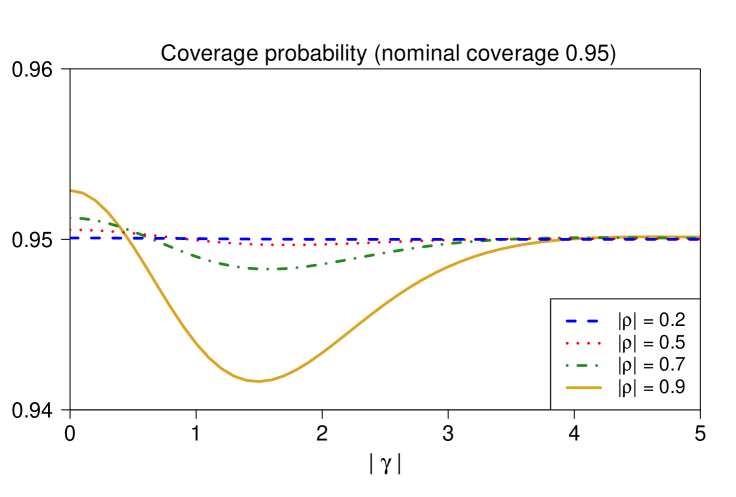
Figure 1 is the graph of coverage probability of the confidence interval $J_{\rm delta}$ centered on the bootstrap smoothed estimator, which is based on the post-model-selection estimator obtained after a preliminary hypothesis test, with size $\widetilde{\alpha}=0.1$, of the null hypothesis that the simpler model is correct. We consider the case that the nominal coverage is 0.95, $n=25$, $m=1$ and $|\rho|=0.2,0.5,0.7$ and 0.9. All of the computations reported in this paper were carried out using programs written in R. The minimum coverage probability of this CI is a continuous decreasing function of $|\rho|$ which equals the nominal coverage when $\rho=0$. Graphs of the coverage probability of $J_{\rm delta}$ for the same values of nominal coverage, size of the preliminary hypothesis test, $n$ and $|\rho|$ are provided in the Supporting Material for $m=2,3$ and 10. Further extensive numerical investigations, not reported either here or in the Supporting Material, show that the ${\bf sd}_{\rm delta}\,{\bf interval}$ outperforms the post-model-selection CI, with the same nominal coverage and based on the same preliminary test, in terms of coverage probability.

Refer to caption
Figure 1: The coverage probability of the ${\bf sd}_{\rm delta}$ interval, which is based on the post-model-selection estimator obtained after a preliminary hypothesis test, with size $0.1$, of the null hypothesis that the simpler model is correct. The nominal coverage is 0.95, $n=25$, $m=1$ and $|\rho|=0.2,0.5,0.7$ and 0.9.

5. Computationally convenient exact formula for the scaled expected length of the confidence interval centered on the bootstrap smoothed estimator

We define the scaled expected length of $J_{\rm delta}$, with nominal coverage $1-\alpha$, to be the expected length of $J_{\rm delta}$ divided by the expected length of the usual CI, based on the full model, with the same coverage as the minimum coverage probability of $J_{\rm delta}$. Let $c_{\rm min}$ denote this minimum coverage probability. Now let $I(c)$ denote the usual CI for $\theta$, with coverage probability $c$, based on the full model. In other words, $I(c)=\Big{[}\widehat{\theta}-t_{m}(1-c)\,\widehat{\sigma}\,v_{\theta}^{1/2},\,\widehat{\theta}+t_{m}(1-c)\,\widehat{\sigma}\,v_{\theta}^{1/2}\Big{]}$. It may be shown that the scaled expected length of $J_{\rm delta}$ is a function of $(\gamma,\rho)$. We therefore denote this scaled expected length by ${\rm SEL}_{\rm delta}(\gamma,\rho)$. The following theorem is proved in Appendix A.3.

Theorem 3.

Let $c_{\rm min}$ denote the minimum coverage probability of the confidence interval $J_{\rm delta}$, with nominal coverage $1-\alpha$. Then ${\rm SEL}_{\rm delta}(\gamma,\rho)$ is given by

$$\frac{t_{m}(\alpha)}{t_{m}(1-c_{\rm min})}\,\left(\frac{m}{2}\right)^{1/2}\frac{\Gamma(m/2)}{\Gamma((m+1)/2)}\,\int_{0}^{\infty}\int_{-\infty}^{\infty}w\,\,r_{\rm delta}\left(\frac{y+\gamma}{w}\right)\,\phi(y)\,dy\,f_{W}(w)\,dw.$$

The expression (2) suggests that, for all sufficiently large $n$, ${\rm SEL}_{\rm delta}(\gamma,\rho)$ is determined by $m$, for any given $(\gamma,\rho)$. Computational results for $n=25$ (described later in this section) and $n=100$ (not described either here or in the Supporting Material) suggest that, for all $n\geq 25$, ${\rm SEL}_{\rm delta}(\gamma,\rho)$ is, for practical purposes, determined by $m$, for any given $(\gamma,\rho)$. It may be shown that ${\rm SEL}_{\rm delta}(\gamma,\rho)$ is (a) an even function of $\gamma$ for each $\rho$ and (b) an even function of $\rho$ for each $\gamma$. It follows that, for given $n$ and $m$, we are able to encapsulate the scaled expected length of the ${\bf sd}_{\rm delta}\,{\bf interval}$, for all possible choices of design matrix, parameter of interest $\theta$ and parameter $\tau$ that specifies the simpler model, using only the parameters $|\rho|$ and $|\gamma|$.

The bootstrap smoothed estimator is obtained by smoothing the post-model-selection estimator that results from a preliminary test of the null hypothesis that the simpler model is correct i.e. that $\gamma=0$. This post-model-selection estimator is usually motivated by a desire for good performance when the simpler model is correct. Therefore, ideally, the ${\bf sd}_{\rm delta}\,{\bf interval}$ should have a scaled expected length that is substantially less than 1 when $\gamma=0$. In addition, ideally, this confidence interval should have a scaled expected length that (a) has maximum value that is not too much larger than 1 and (b) approaches 1 as $|\gamma|$ approaches infinity.

Figure 2 is the graph of scaled expected length of the confidence interval centered on the bootstrap smoothed estimator, which is based on the post-model-selection estimator obtained after a preliminary hypothesis test, with size $\widetilde{\alpha}=0.1$, of the null hypothesis that the simpler model is correct. We consider the case that the nominal coverage is 0.95, $n=25$, $m=1$ and $|\rho|=0.2,0.5,0.7$ and 0.9. For $|\rho|=0.5,0.7$ and 0.9, the scaled expected length is substantially less than 1 when $\gamma=0$. In addition, the scaled expected length (a) has maximum value that is not too much larger than 1 and (b) approaches 1 as $|\gamma|$ approaches infinity. This shows that for $m=1$ and $|\rho|\geq 0.5$ the scaled expected length of ${\bf sd}_{\rm delta}$ interval has the desired properties. This finding is similar to that reported in Kabaila and Giri (2013) concerning the performance of the CIs constructed by Kabaila and Giri (2009) to have the desired coverage probability and these desired scaled expected length properties. Namely, the performance of this CI improves as $|\rho|$ increases and $m$ decreases.

By contrast, for the case that $\sigma^{2}$ is assumed known, examined by Kabaila and Wijethunga (2019), the scaled expected length of the CI centered on the bootstrap smoothed estimator (a) is either greater than 1 or only slightly less than 1 at $\gamma=0$ and (b) has maximum value that is an increasing function of $|\rho|$ that can be much larger than 1 for large $|\rho|$. As noted earlier, we expect that as $m$ increases (which implies that $n$ also increases), the results obtained in the present paper will approach the corresponding results obtained by Kabaila and Wijethunga (2019). Therefore we expect that as $m$ increases the ${\bf sd}_{\rm delta}$ interval will get further and further away from possessing the desired scaled expected length properties. This is confirmed by the graphs of the scaled expected length of $J_{\rm delta}$ for nominal coverage 0.95, size $\widetilde{\alpha}=0.1$ of the preliminary hypothesis test, $n=25$ and $|\rho|\in\{0.2,0.5,0.7,0.9\}$ that are provided in the Supporting Material for $m=2,3$ and 10.

Refer to caption
Figure 2: The scaled expected length of the ${\bf sd}_{\rm delta}$ interval, which is based on the post-model-selection estimator obtained after a preliminary hypothesis test, with size $0.1$, of the null hypothesis that the simpler model is correct. The nominal coverage is 0.95, $n=25$, $m=1$ and $|\rho|=0.2,0.5,0.7$ and 0.9.

6. Discussion

For the test scenario of two nested linear regression models and error variance assumed known, Kabaila and Wijethunga (2019) found that the ${\bf sd}_{\rm delta}$ interval does not perform any better in terms of expected length than the usual confidence interval, with the same minimum coverage probability and based on the full model. Intuitively, the case that the error variance is assumed to be known corresponds to the case that the error variance is unknown (so that it must be estimated) and the number of degrees of freedom $m$ for the estimation of the error variance is large.

In the present paper, we deal with the case that the error variance is unknown. We find that, for small $m$ and large magnitude of correlation between the least squares estimators of the parameter of interest and the parameter that is set to zero to specify the simpler model, the expected length of the ${\bf sd}_{\rm delta}$ interval possesses some attractive features.

Acknowledgement

This work was supported by an Australian Government Research Training Program Scholarship.

References

  • Akaike (1974) Akaike, H., 1974. A new look at statistical model identification. IEEE Transactions on Automatic Control 19, 716–723.
  • Barndorff-Nielsen and Cox (1989) Barndorff-Nielsen, O.E., Cox, D.R., 1989. Asymptotic Techniques for Use in Statistics. Chapman & Hall, London.
  • Barndorff-Nielsen and Cox (1994) Barndorff-Nielsen, O.E., Cox, D.R., 1994. Inference and Asymptotics. Chapman & Hall, London.
  • Breiman (1996) Breiman, L., 1996. Bagging predictors. Machine Learning 24, 123–140.
  • Buckland etΒ al. (1997) Buckland, S.T., Burnham, K.P., Augustin, N.H., 1997. Model selection: an integral part of inference. Biometrics 53, 603–618.
  • Efron (2014) Efron, B., 2014. Estimation and accuracy after model selection. Journal of the American Statistical Association 109, 991–1007.
  • Fletcher and Turek (2011) Fletcher, D., Turek, D., 2011. Model-averaged profile likelihood intervals. Journal of Agricultural, Biological, and Environmental Statistics 17, 38–51.
  • Kabaila (2009) Kabaila, P., 2009. The coverage properties of confidence regions after model selection. International Statistical Review 77, 405–414.
  • Kabaila and Giri (2009) Kabaila, P., Giri, K., 2009. Confidence intervals in regression utilizing prior information. Journal of Statistical Planning and Inference 139, 3419–3429.
  • Kabaila and Giri (2013) Kabaila, P., Giri, K., 2013. Further properties of frequentist confidence intervals in regression that utilize uncertain prior information. Australian & New Zealand Journal of Statistics 55, 259–270.
  • Kabaila etΒ al. (2016) Kabaila, P., Welsh, A.H., Abeysekera, W., 2016. Model-averaged confidence intervals. Scandinavian Journal of Statistics 43, 35–48.
  • Kabaila etΒ al. (2017) Kabaila, P., Welsh, A.H., Mainzer, R., 2017. The performance of model averaged tail area confidence intervals. Communications in Statistics - Theory and Methods 46, 10718–10732.
  • Kabaila and Wijethunga (2019) Kabaila, P., Wijethunga, C., 2019. Confidence intervals centred on bootstrap smoothed estimators. Australian & New Zealand Journal of Statistics doi:10.1111/anzs.12252.
  • Leeb and PΓΆtscher (2005) Leeb, H., PΓΆtscher, B.M., 2005. Model selection and inference: facts and fiction. Econometric Theory 21, 21–59.
  • Turek and Fletcher (2012) Turek, D., Fletcher, D., 2012. Model-averaged wald confidence intervals. Computational Statistics & Data Analysis 56, 2809–2815.

Appendix

Let $\widetilde{\gamma}=\widehat{\tau}/(\sigma{v_{\tau}}^{1/2})$, so that $\widehat{\gamma}=\widetilde{\gamma}/W$, where $W=\widehat{\sigma}/\sigma$. Note that $(\widehat{\theta},\widetilde{\gamma})$ and $W$ are independent and $W$ has the same distribution as $(Q/m)^{1/2}$ where $Q\sim\chi^{2}_{m}$. To find convenient formulas for expectations and probabilities of interest, we will express all quantities of interest in terms of $W$ and the random vector $\big{(}\widehat{\theta},\widetilde{\gamma}\big{)}$, which has a bivariate normal distribution with mean $(\theta,\gamma)$ and known covariance matrix with diagonal elements 1 and off-diagonal elements $\rho$.

A1. Outline of the Proof of Theorem 1

For the sake of brevity, we present only an outline of the proof of Theorem 1. By (1.6) of Barndorff-Nielsen and Cox (1994), the pdf of $\bm{y}$ can be expressed in the exponential family form $h(\bm{y})\exp\big{(}\widehat{\bm{s}}^{\top}\bm{\eta}-\psi(\bm{\eta})\big{)}$, where $\widehat{\bm{s}}$ is a sufficient statistic and $\bm{\eta}$ is the unknown parameter vector, with

$\displaystyle\widehat{\bm{s}}=\left[\begin{array}[]{c}\bm{y}^{\top}\bm{y}\\ \widehat{\bm{\beta}}\end{array}\right],\quad\bm{\eta}=\left[\begin{array}[]{c}-1/(2\sigma^{2})\\ \bm{X}^{\top}\bm{X}\bm{\beta}/\sigma^{2}\end{array}\right]\quad\text{and}\quad\psi(\bm{\eta})=\frac{\bm{\beta}^{\top}\bm{X}^{\top}\bm{X}\bm{\beta}}{2\sigma^{2}}+\frac{n}{2}\log(\sigma^{2}).$

For any two random vectors $\bm{u}$ and $\bm{v}$, define $\mbox{$\textrm{{cov}}$}(\bm{u},\bm{v})=E\big{(}(\bm{u}-E(\bm{u}))(\bm{v}-E(\bm{v}))^{\top}\big{)}$. By Theorem 2 of Efron (2014), the ideal delta method approximation to the standard deviation of $\widetilde{\theta}$, which we denote by ${\bf sd}_{\rm delta}$, is given by

$${\bf sd}_{\rm delta}=\Big{(}\big{(}\mbox{$\textrm{{cov}}$}_{*}(\bm{\eta})\big{)}^{\top}\,\big{(}V(\bm{\eta})\big{)}^{-1}\,\mbox{$\textrm{{cov}}$}_{*}(\bm{\eta})\Big{)}^{1/2},$$ (7)

where $\mbox{$\textrm{{cov}}$}_{*}(\bm{\eta})=\mbox{$\textrm{{cov}}$}\big{(}\widehat{\bm{s}},\,\widehat{\theta}_{\textsc{\tiny PMS}}\big{)}$ and

$\displaystyle V(\bm{\eta})$ $\displaystyle=\mbox{$\textrm{{cov}}$}(\widehat{\bm{s}})=\mbox{$\textrm{{cov}}$}\left[\begin{array}[]{c}\bm{y}^{\top}\bm{y}\\ \widehat{\bm{\beta}}\end{array}\right]=\left[\vbox{\hbox{\kern-1.15198pt\raise 0.0pt\hbox{\kern 93.97986pt}\kern 0.0pt\vbox{}\kern-1.15198pt}}\right]$

Now $\bm{y}^{\top}\bm{y}-E(\bm{y}^{\top}\bm{y})=2\bm{\beta}^{\top}\bm{X}^{\top}\bm{\varepsilon}+\bm{\varepsilon}^{\top}\bm{\varepsilon}-n\sigma^{2}$. Thus

$\displaystyle\mbox{$\textrm{{var}}$}(\bm{y}^{\top}\bm{y})$ $\displaystyle=E\left(\Big{(}\bm{q}^{\top}\bm{\varepsilon}+\sum_{i=1}^{n}(\varepsilon_{i}^{2}-\sigma^{2})\Big{)}^{2}\right),\quad\text{where}\quad\bm{q}^{\top}=2\bm{\beta}^{\top}\bm{X}^{\top},$
$\displaystyle=4\sigma^{2}\bm{\beta}^{\top}\bm{X}^{\top}\bm{X}\bm{\beta}+2n\sigma^{4}.$

Also, $\mbox{$\textrm{{cov}}$}\big{(}\bm{y}^{\top}\bm{y},\widehat{\bm{\beta}}\big{)}=2\sigma^{2}\bm{\beta}^{\top}$. Thus

$\displaystyle V(\bm{\eta})=\sigma^{2}\left[\vbox{\hbox{\kern-1.15198pt\raise 0.0pt\hbox{\kern 109.17337pt}\kern 0.0pt\vbox{}\kern-1.15198pt}}\right]$

Hence

$$\big{(}V(\bm{\eta})\big{)}^{-1}=\frac{1}{\sigma^{2}}\left[\vbox{\hbox{\kern-1.15198pt\raise 0.0pt\hbox{\kern 151.02101pt}\kern 0.0pt\vbox{}\kern-1.15198pt}}\right].$$ (11)

Let $\bm{s}=E(\bm{\widehat{s}})$ and observe that $\mbox{$\textrm{{cov}}$}_{*}(\bm{\eta})$ is equal to

$\displaystyle E\Big{(}\big{(}\widehat{\bm{s}}-\bm{s}\big{)}\big{(}\widehat{\theta}_{\textsc{\tiny PMS}}-\theta\big{)}\Big{)}$
$\displaystyle=E\Big{(}\big{(}\widehat{\bm{s}}-\bm{s}\big{)}\big{(}\widehat{\theta}-\theta\big{)}\Big{)}-\rho\,\sigma\,v_{\theta}^{1/2}\int_{0}^{\infty}\int_{-d_{m}w}^{d_{m}w}z\,E\big{(}\widehat{\bm{s}}-\bm{s}\big{|}\widetilde{\gamma}=z\big{)}\phi(z-\gamma)\,dz\,f_{W}(w)\,dw$

where $d_{m}=t_{m}(\widetilde{\alpha})$. It may be shown that

$\displaystyle E\Big{(}\big{(}\widehat{\bm{s}}-\bm{s}\big{)}\big{(}\widehat{\theta}-\theta\big{)}\Big{)}=\sigma^{2}\left[\begin{array}[]{c}2\,\theta\\ v_{\theta}\\ \rho\,v_{\theta}^{1/2}\,v_{\tau}^{1/2}\\ \bm{0}\end{array}\right]$

and

$\displaystyle E\big{(}\widehat{\bm{s}}-\bm{s}\big{|}\widetilde{\gamma}=z\big{)}$ $\displaystyle=\left[\begin{array}[]{c}E\Big{(}\mbox{$\bm{y}$}^{\top}\mbox{$\bm{y}$}-E\big{(}\mbox{$\bm{y}$}^{\top}\mbox{$\bm{y}$}\big{)}\,\Big{|}\,\widetilde{\gamma}=z\Big{)}\\ \sigma(z-\gamma)\left[\begin{array}[]{c}\rho\,v_{\theta}^{1/2}\\ v_{\tau}^{1/2}\\ \bm{0}\end{array}\right]\end{array}\right]$
$\displaystyle=\left[\begin{array}[]{c}\sigma^{2}\Big{(}2\gamma(z-\gamma)+(z-\gamma)^{2}-1\Big{)}\\ \sigma(z-\gamma)\left[\begin{array}[]{c}\rho\,v_{\theta}^{1/2}\\ v_{\tau}^{1/2}\\ \bm{0}\end{array}\right]\end{array}\right].$

It may also be shown, using the definitions of the Hermite polynomials of degrees 1, 2 and 3 (given e.g. by Barndorff-Nielsen and Cox, 1989), that

$\displaystyle\int_{0}^{\infty}\int_{-d_{m}w}^{d_{m}w}z\,E\big{(}\widehat{\bm{s}}-\bm{s}\big{|}\widetilde{\gamma}=z\big{)}\phi(z-\gamma)dz\,f_{W}(w)\,dw$
$\displaystyle\qquad\qquad\qquad\qquad=\sigma\left[\begin{array}[]{c}\sigma\Big{(}\gamma\,q_{m}(\gamma)+k_{m}(\gamma)+h_{m}(\gamma)\Big{)}\\ \rho\,v_{\theta}^{1/2}q_{m}(\gamma)\\ v_{\tau}^{1/2}q_{m}(\gamma)\\ \bm{0}\end{array}\right],$

where the functions $k_{m}$, $q_{m}$ and $h_{m}$ are defined by (1), (3) and (4), respectively. Thus

$$\mbox{$\textrm{{cov}}$}_{*}(\bm{\eta})=\sigma^{2}\left[\begin{array}[]{c}2\theta-\rho\,\sigma v_{\theta}^{1/2}\Big{(}\gamma\,q_{m}(\gamma)+k_{m}(\gamma)+h_{m}(\gamma)\Big{)}\\ v_{\theta}\,\big{(}1-\rho^{2}\,q_{m}(\gamma)\big{)}\\ \rho\,v_{\theta}^{1/2}v_{\tau}^{1/2}\big{(}1-q_{m}(\gamma)\big{)}\\ \bm{0}\end{array}\right].$$

The result now follows from (7) and (11).

∎

A2. Proof of Theorem 2

Let $G=(\widehat{\theta}-\theta)/(\sigma\,v_{\theta}^{1/2})$. The coverage probability of the ${\bf sd}_{\rm delta}$ interval is

$\displaystyle P\left(\widetilde{\theta}-t_{m}(\alpha)\,{\bf sd}_{\rm delta}(\widehat{\gamma},\widehat{\sigma})\leq\theta\leq\widetilde{\theta}+t_{m}(\alpha)\,{\bf sd}_{\rm delta}(\widehat{\gamma},\widehat{\sigma})\right)$
$\displaystyle=P\left(-t_{m}(\alpha)\,\frac{{\bf sd}_{\rm delta}(\widehat{\gamma},\widehat{\sigma})}{\widehat{\sigma}\,v_{\theta}^{1/2}}\leq\frac{\widehat{\theta}-\theta}{\widehat{\sigma}\,v_{\theta}^{1/2}}-\rho\,k_{m}(\widehat{\gamma})\leq t_{m}(\alpha)\,\frac{{\bf sd}_{\rm delta}(\widehat{\gamma},\widehat{\sigma})}{\widehat{\sigma}\,v_{\theta}^{1/2}}\right)$
$\displaystyle=P\left(-t_{m}(\alpha)\,r_{\rm delta}(\widehat{\gamma})\leq\frac{G}{W}-\rho\,k_{m}(\widehat{\gamma})\leq t_{m}(\alpha)\,r_{\rm delta}(\widehat{\gamma})\right)$
$\displaystyle=P\Bigg{(}-t_{m}(\alpha)\,r_{\rm delta}\left(\frac{\widetilde{\gamma}}{W}\right)\leq\frac{G}{W}-\rho\,k_{m}\left(\frac{\widetilde{\gamma}}{W}\right)\leq t_{m}(\alpha)\,r_{\rm delta}\left(\frac{\widetilde{\gamma}}{W}\right)\Bigg{)}$
$\displaystyle=\int_{0}^{\infty}\int_{-\infty}^{\infty}P\Bigg{(}-t_{m}(\alpha)\,r_{\rm delta}\left(\frac{\widetilde{\gamma}}{W}\right)\leq\frac{G}{W}-\rho\,k_{m}\left(\frac{\widetilde{\gamma}}{W}\right)\leq t_{m}(\alpha)\,r_{\rm delta}\left(\frac{\widetilde{\gamma}}{W}\right)\Bigg{|}$
$\displaystyle\qquad\qquad\qquad\qquad\qquad\qquad\qquad\qquad\qquad\widetilde{\gamma}=h,W=w\Bigg{)}\phi(h-\gamma)\,dh\,f_{W}(w)\,dw.$

By the substitution theorem for conditional expectations and since $G$ and $W$ are independent random variables, this is equal to

$\displaystyle\int_{0}^{\infty}\int_{-\infty}^{\infty}P\Bigg{(}-t_{m}(\alpha)\,r_{\rm delta}\left(\frac{h}{w}\right)\leq\frac{G}{w}-\rho\,k_{m}\left(\frac{h}{w}\right)\leq t_{m}(\alpha)\,r_{\rm delta}\left(\frac{h}{w}\right)\Bigg{|}\widetilde{\gamma}=h\Bigg{)}$
$\displaystyle\qquad\qquad\qquad\qquad\qquad\qquad\qquad\qquad\qquad\qquad\qquad\qquad\qquad\phi(h-\gamma)\,dh\,f_{W}(w)\,dw.$

Obviously

$\displaystyle P\Bigg{(}-t_{m}(\alpha)\,r_{\rm delta}\left(\frac{h}{w}\right)\leq\frac{G}{w}-\rho\,k_{m}\left(\frac{h}{w}\right)\leq t_{m}(\alpha)\,r_{\rm delta}\left(\frac{h}{w}\right)\Bigg{|}\widetilde{\gamma}=h\Bigg{)}$
$\displaystyle=P\Big{(}\ell(h,w,\rho)\leq G\leq u(h,w,\rho)\Big{|}\widetilde{\gamma}=h\Big{)},$

where the functions $\ell$ and $u$ are defined by (5) and (6), respectively. The distribution of $G$, conditional on $\widetilde{\gamma}=h$, is $N\big{(}\rho(h-\gamma),1-\rho^{2}\big{)}$. Thus $P\big{(}\ell(h,w,\rho)\leq G\leq u(h,w,\rho)\,\big{|}\,\widetilde{\gamma}=h\big{)}=P\big{(}\ell(h,w,\rho)\leq\widetilde{G}\leq u(h,w,\rho)\big{)}$, where $\widetilde{G}\sim N\big{(}\rho(h-\gamma),1-\rho^{2}\big{)}$. Therefore the coverage probability $\rm CP_{\rm delta}(\gamma,\rho)$ is equal to

$\displaystyle\int_{0}^{\infty}\int_{-\infty}^{\infty}\Psi\Big{(}\ell(h,w,\rho),u(h,w,\rho);\rho(h-\gamma),1-\rho^{2}\Big{)}\phi(h-\gamma)\,dh\,f_{W}(w)\,dw.$

The result follows by changing the variable of integration of the inner integral to $y=h-\gamma$.

∎

A3. Proof of Theorem 3

The scaled expected length $\rm SEL_{\rm delta}(\gamma,\rho)=E\big{(}\text{length of }J_{\rm delta}\big{)}\big{/}E\big{(}\text{length of }I(c_{\rm min})\big{)}$. The length of $J_{\rm delta}$ is $2\,t_{m}(\alpha)\,{\bf sd}_{\rm delta}(\widehat{\gamma},\widehat{\sigma})$. Thus

$\displaystyle E\big{(}\text{length of }J_{\rm delta}\big{)}=2\,t_{m}(\alpha)\,\sigma\,v_{\theta}^{1/2}\,E\left(W\,\,r_{\rm delta}\Big{(}\frac{\widetilde{\gamma}}{W}\Big{)}\right).$

The expected length of $I(c_{\rm min})$ is

$\displaystyle E\left(2\,t_{m}(1-c_{\rm min})\,\widehat{\sigma}\,v_{\theta}^{1/2}\right)=2\,t_{m}(1-c_{\rm min})\,\sigma\,v_{\theta}^{1/2}\,E\left(W\right).$

Hence the scaled expected length is

$\displaystyle{\rm SEL}_{\rm delta}(\gamma,\rho)=\frac{t_{m}(\alpha)}{t_{m}(1-c_{\rm min})}\,\frac{E\left(W\,\,\displaystyle r_{\rm delta}\Big{(}\frac{\widetilde{\gamma}}{W}\Big{)}\right)}{E\left(W\right)}.$

Since $W$ has the same distribution as $(Q/m)^{1/2}$, where $Q\sim\chi^{2}_{m}$,

$\displaystyle E(W)=\left(\frac{m}{2}\right)^{-1/2}\,\frac{\Gamma((m+1)/2)}{\Gamma(m/2)}.$

Hence

$\displaystyle\rm SEL_{\rm delta}(\gamma,\rho)$
$\displaystyle=\frac{t_{m}(\alpha)}{t_{m}(1-c_{\rm min})}\,\left(\frac{m}{2}\right)^{1/2}\,\frac{\Gamma(m/2)}{\Gamma((m+1)/2)}\,\int_{0}^{\infty}\int_{-\infty}^{\infty}w\,r_{\rm delta}\left(\frac{h}{w}\right)\,\phi(h-\gamma)\,dh\,f_{W}(w)\,dw.$

The result follows by changing the variable of integration of the inner integral to $y=h-\gamma$.

∎