Dust traps in the protoplanetary disc MWC 758:
two vortices produced by two giant planets?

Abstract

Resolved ALMA and VLA observations indicate the existence of two dust traps in the protoplanetary disc MWC 758. By means of 2D gas+dust hydrodynamical simulations post-processed with 3D dust radiative transfer calculations, we show that the spirals in scattered light, the eccentric, asymmetric ring and the crescent-shaped structure in the (sub)millimetre can all be caused by two giant planets: a 1.5-Jupiter mass planet at 35 au (inside the spirals) and a 5-Jupiter mass planet at 140 au (outside the spirals). The outer planet forms a dust-trapping vortex at the inner edge of its gap (at $\sim$85 au), and the continuum emission of this dust trap reproduces the ALMA and VLA observations well. The outer planet triggers several spiral arms which are similar to those observed in polarised scattered light. The inner planet also forms a vortex at the outer edge of its gap (at $\sim$50 au), but it decays faster than the vortex induced by the outer planet, as a result of the disc’s turbulent viscosity. The vortex decay can explain the eccentric inner ring seen with ALMA as well as the low signal and larger azimuthal spread of this dust trap in VLA observations. Finding the thermal and kinematic signatures of both giant planets could verify the proposed scenario.

1 Introduction

MWC 758 is a 3.5 $\pm$ 2.0 Myr Herbig A5 star (Meeus et al., 2012) located at a distance of 160.2 $\pm$ 1.7 pc (Gaia Collaboration et al., 2018). Its mass has been estimated as 1.5 $\pm$ 0.2 $M_{\odot}$ (Isella et al., 2010; Reggiani et al., 2018). The disc around MWC 758 is a transition disc with a nearly 50 au (0$\aas@@fstack{\prime\prime}$30) cavity in the submillimetre (Andrews et al., 2011). Recent high angular resolution observations have revealed stunning non-axisymmetric emission features in the MWC 758 disc. These asymmetries so far consist of multiple spiral arms and arcs in near-infrared scattered light (Grady et al., 2013; Benisty et al., 2015; Reggiani et al., 2018; Ren et al., 2018), an asymmetric ring of emission at $\sim$0$\aas@@fstack{\prime\prime}$32 as well as a compact crescent-shaped structure at $\sim$0$\aas@@fstack{\prime\prime}$53 in the (sub)millimetre emission (Marino et al., 2015; Boehler et al., 2018; Dong et al., 2018; Casassus et al., 2019). The asymmetries in the (sub)millimetre emission, which we will refer to as Clump 1 (crescent at $\sim$0$\aas@@fstack{\prime\prime}$53) and Clump 2 (asymmetric ring at $\sim$0$\aas@@fstack{\prime\prime}$32; see the right-hand panels in Fig. 4) have been interpreted as dust traps at local pressure maxima arising from two large-scale vortices (Marino et al., 2015). The cm-wavelength VLA observations presented in Casassus et al. (2019) support the dust trapping scenario for Clump 1, and suggest marginal trapping for Clump 2. Still, the mechanism behind the formation of the possible dust-trapping vortices in the MWC 758 disc remains elusive and is the subject of this paper.

One way to form a large-scale vortex in a protoplanetary disc is through the Rossby wave instability (RWI; Lovelace et al., 1999; Li et al., 2000, 2001). This instability can set in when there is a radial minimum in the gas vortensity, which in practice may occur where there is a radial pressure bump. A radial pressure bump can form for instance at the transition between magnetically active and inactive regions in protoplanetary discs, where a sharp transition in the effective turbulent viscosity occurs (Varnière & Tagger, 2006; Regály et al., 2012; Lyra et al., 2015), or at the edges of the gap that a massive planet carves in its disc (e.g., Lyra et al., 2009; Lin, 2012). More often, it is the gap’s outer edge that develops a pressure maximum, but a very massive planet of typically a few Jupiter masses may also form and maintain a pressure maximum at the inner edge of its gap (Bae et al., 2016).

Whatever its trigger, the RWI leads to the formation of one or several vortices, which tend to merge and form a single large-scale anticyclonic vortex. An anticyclonic vortex forms a patch of closed elliptical streamlines about a local pressure maximum. The vortex flow tends to maintain dust on the same elliptical streamlines, gas drag tends to drive dust towards the vortex centre, while dust turbulent diffusion tends to spread it out (Chavanis, 2000; Youdin, 2010; Lyra & Lin, 2013). In addition, the vortex’s self-gravity causes dust particles to describe horseshoe U-turns relative to the vortex centre, much like in the circular restricted three-body problem, despite the vortex not being a point mass (Baruteau & Zhu, 2016). The competition between the aforementioned effects implies that dust particles of increasing size get trapped farther ahead of the vortex centre in the azimuthal direction (Baruteau & Zhu, 2016). Vortices triggered by the RWI could play a key role in planet formation by slowing down or stalling the dust’s inward drift due to gas drag, while potentially allowing dust to grow to planetesimal sizes or even planetary sizes (Lyra et al., 2009; Sándor et al., 2011).

A planetary origin for the two possible vortices in the MWC 758 disc is appealing as it could also account for the detection of a point-like source inside the submillimetre cavity in the $L^{\prime}$-band high-contrast imaging observations of Reggiani et al. (2018), and for the spirals in near-infrared scattered light. The aim of this paper is to present theoretical support for the scenario where the asymmetric structures in the (sub)millimetre and the spirals in scattered light could be due to the presence of two massive planets in the MWC 758 disc. For this purpose, we have carried out two-dimensional (2D) gas+dust hydrodynamical simulations of the protoplanetary disc around MWC 758, and used 3D dust radiative transfer calculations to compare synthetic maps of continuum and scattered light with observations. In Section 2, we describe the physical model and numerical setup of the hydrodynamical simulations and the radiative transfer calculations. Their results are then presented in Section 3. Discussion and summary follow in Section 4.

2 Physical model and numerical methods

2.1 Hydrodynamical simulations

We carried out 2D gas+dust hydrodynamical simulations using the code Dusty FARGO-ADSG. It is an extended version of the grid-based code FARGO-ADSG (Masset, 2000; Baruteau & Masset, 2008a, b) with dust modelled as Lagrangian test particles (Baruteau & Zhu, 2016; Fuente et al., 2017).

2.1.1 Planets

We assume that MWC 758, which we take as a $M_{\star}=1.5M_{\odot}$ star (Isella et al., 2010; Reggiani et al., 2018), has two planetary companions: a 1.5 Jupiter-mass planet at 35 au, and a 5 Jupiter-mass planet at 140 au. The mass of the inner planet is chosen such that it opens a mild gap in the gas around its orbit (see first paragraph in Section 3.1), to be consistent with the non-detection of a gap in scattered light around this location ($\sim$0$\aas@@fstack{\prime\prime}$22, Benisty et al., 2015). The mass of the outer planet is taken as the upper mass limit for a companion at this location ($\sim$0$\aas@@fstack{\prime\prime}$87), as estimated by Reggiani et al. (2018) based on their $L^{\prime}$-band observations and the use of the BT-Settl hot start evolutionary model for planetary luminosities at near-infrared wavelengths (Allard, 2014). Section 4.4 contains a discussion on the location and mass of the possible planets in the MWC 758 disc. In our simulations, the planets do not migrate in the disc (they remain on quasi-circular orbits). To avoid a violent relaxation of the disc due to the sudden introduction of the planets, their mass is gradually increased over 20 orbits of the inner planet. In the following, whenever time is expressed in orbits, it refers to the orbital period at the inner planet’s location, which is about 170 yr.

2.1.2 Gas

A locally isothermal equation of state is assumed for the gas, where its temperature remains fixed in time. Based on Boehler et al. (2018)’s thermal Monte Carlo simulation of the MWC 758 disc (see their figure 9), we take the midplane temperature to decrease as $r^{-1}$ and equal to 85 K at 35 au ($r$ denotes the radial cylindrical coordinate measured from the central star). The disc’s aspect ratio $h$, which is the ratio of the midplane isothermal sound speed to the Keplerian velocity, is therefore uniform and equal to 0.088 (we assume a mean molecular weight of 2.4).

The initial surface density of the disc gas, which we denote by $\Sigma_{0}$, is assumed proportional to $r^{-1}$ and equal to $\sim$1.7 g cm^-2 at 35 au. In a quasi steady state, when the planets have carved a gap around their orbit, the azimuthally-averaged gas surface density varies from 1 to 2 g cm^-2 between 40 and 90 au, which is overall consistent with the values of the gas surface density obtained by Boehler et al. (2018) based on their ALMA band 7 observations of ¹³CO and C¹⁸O in the MWC 758 disc (see their Figure 8). Despite the Toomre $Q$-parameter being rather large (it is $\sim$30 at 85 au, the radial location of Clump 1), gas self-gravity is included, as it is found to impact both the vortex lifetime (Zhu & Baruteau, 2016; Regály & Vorobyov, 2017) and the dust dynamics (Baruteau & Zhu, 2016) given our range of disc parameters. The importance of gas self-gravity will be further emphasised in Section 4.1. To mimic the effect of a finite vertical thickness, a softening length of $0.3H(r)$ is used in the calculation of the self-gravitating acceleration, with $H(r)=h\times r$ the disc’s pressure scale height. Likewise, a softening length of $0.6H(r)$ is used in the calculation of the planets acceleration on the gas.

Turbulent transport of angular momentum is modelled by a constant alpha turbulent viscosity, $\alpha=10^{-4}$. This rather low level of turbulence is representative of the discs midplane from a few tens to a hundred au, as suggested by observations of the dust continuum in the submillimetre (see, e.g., Pinte et al., 2016, for the modelling of the HL Tau disc), and according to 3D, non-ideal, local magnetohydrodynamic (MHD) simulations (although larger $\alpha$ values in the midplane can be obtained depending on the disc model, in particular the amplitude of the vertical magnetic field that threads the disc, see, e.g., Simon et al., 2015, 2018).

The continuity and momentum equations for the gas are solved on a polar grid centred on the star, and the indirect terms due to the acceleration of the star by the disc and the planets are taken into account. The grid extends from 10.5 au to 350 au in the radial direction, and from 0 to $2\pi$ in the azimuthal direction. We use 900 cells in the radial direction with a logarithmic spacing (required for the gas self-gravitating acceleration to be computed by Fast-Fourier Transforms; see Baruteau & Masset, 2008b). We use 1200 cells evenly spaced in azimuth. Given our initial surface density profile, the initial mass of the disc gas amounts to $\sim$0.01 $M_{\star}$. To minimise the reflection of the planets wakes, we use wave-killing zones as boundary conditions at the inner and outer radial edges of the grid, where the disc fields are damped towards their initial value. We have checked that a different choice of boundary condition does not affect our results.

2.1.3 Dust

Dust is modelled as Lagrangian test particles that feel the gravity of the star, of the planets, of the gaseous disc (since gas self-gravity is included), and gas drag. Dust turbulent diffusion is also included as stochastic kicks on the particles position following the method in Charnoz et al. (2011) (see Ataiee et al., 2018 for more details). However, the dust self-gravity, dust drag (or feedback), growth and fragmentation are not taken into account in the simulations.

We use 10⁵ particles with a size distribution $n_{\rm simu}(s)\propto s^{-1}$ for the particles size $s$ ranging from 10 $\mu$m to 10 cm (the quantity $n_{\rm simu}(s)ds$ represents the number of super-particles in the size interval $[s,s+ds]$ in the simulation). This particular scaling of the dust’s size distribution is chosen for computational reasons, as it implies that there is approximately the same number of particles per decade of size. An important note is that the radiative transfer calculations do need a realistic size distribution for the dust, but the only input that they need from the hydrodynamical simulations is the spatial distribution of the dust particles. This is the reason why we can choose any size distribution in the simulations, as long as there is enough particles per bin size to properly resolve their dynamics.

The dust particles are introduced in the disc gas at $300$ orbits after the beginning of the simulation, when the planets have already started to open a gap around their orbit. The particles are uniformly distributed between $52$ au and $102$ au, so that they approximately all remain between the gaps over the duration of the simulation. This is meant to maximise the particles resolution at the two dust traps from which Clump 1 and Clump 2 originate in our scenario. Furthermore, inspired by the dust trapping predictions of Casassus et al. (2019, see their Section 3.2.2), we assume that the dust particles have an internal density $\rho_{\rm int}=0.1$ g cm^-3, independent of particles size, instead of a more conventional internal density of a few g cm^-3. Our dust particles can therefore be considered as moderately porous particles. This rather low density is overall consistent with the collection by Rosetta of large (>10 $\mu$m) porous aggregate particles in the near coma of comet 67P/Churyumov-Gerasimenko (Bentley et al., 2016; Langevin et al., 2016). A brief discussion on how the particles internal density impacts our results is given in Section 4.3.3.

The dust particles that we simulate are much smaller than the mean free path in our disc model, and the Epstein regime of drag is therefore relevant. In this regime, the particle’s Stokes number (St), which is the ratio of the particle’s stopping time to the dynamical time, can be expressed as

$${\rm St}\approx 0.15\times\left(\frac{s}{1\;{\rm cm}}\right)\left(\frac{\rho_{\rm int}}{0.1\;{\rm g\;cm}^{-3}}\right)\left(\frac{1\;{\rm g\;cm}^{-2}}{\Sigma}\right),$$ (1)

where $\Sigma$ denotes here the gas surface density interpolated at the particle’s location. When our simulations reach a quasi steady state, St varies from $\sim$3$\times 10^{-5}$ to $\sim$2. Note that the so-called short-friction time approximation is used in the simulations for the smallest dust particles for which the local stopping time is shorter than the hydrodynamical timestep. A summary of the parameters used in the simulations can be found in Table 1.

Table 1: Simulations parameters

Parameter	Value
Star mass	1.5 M⊙
Inner planet’s mass	1.5 MJup
Inner planet’s location	35 au
Outer planet’s mass	5 MJup
Outer planet’s location	140 au
Disc’s aspect ratio	0.088
Alpha turbulent viscosity	$10^{-4}$
Dust’s initial location	$\in[52-102]$ au
Dust’s size range	$\in[10\,\mu{\rm m}-10\,{\rm cm}]$
Dust’s internal density	0.1 g cm-3

2.2 Radiative transfer calculations

Our results of 2D hydrodynamical simulations are post-processed with the 3D radiative transfer code RADMC3D (version 0.41, Dullemond et al., 2015). The dust’s spatial distribution obtained in our simulations is used as input to compute continuum emission maps at ALMA band 7 (0.9 mm) and VLA (9.0 mm) wavelengths (Section 2.2.1). The gas surface density is used as input to compute a polarised scattered light image in the $Y$-band (1.04 $\mu$m, Section 2.2.2). The spatial grid used in RADMC3D is a 3D extension of the simulations grid in spherical coordinates (the grid’s vertical extent and the number of cells in colatitude are specified in Sections 2.2.1 and 2.2.2). We use $10^{9}$ photon packages for the thermal Monte Carlo calculation of the dust temperature and for the ray-tracing computation of the (sub)millimetre continuum and near-infrared polarised scattered light images. We assume that the star has a radius of 2.0 $R_{\odot}$ and an effective temperature of 7340 K (Gaia Collaboration et al., 2018, or see Gaia archive online). We assume the disc to be located at 160 pc (Gaia Collaboration et al., 2018), with an inclination of $21^{\circ}$ and a position angle of $62^{\circ}$ (Isella et al., 2010; Boehler et al., 2018). Since the disc is rotating clockwise in the observations, but counter-clockwise in the simulation, the effective inclination adopted in the radiative transfer calculations is $201^{\circ}$. The python program used to compute the (sub)millimetre continuum and near-infrared polarised scattered light images with RADMC3D from the results of Dusty FARGO-ADSG simulations, fargo2radmc3d, is publicly available at https://github.com/charango/fargo2radmc3d.

2.2.1 (Sub)millimetre continuum emission

The calculation of the dust’s continuum emission requires to specify (i) the size distribution $n(s)$ and the total mass that the dust which we simulate would have in the MWC 758 disc, (ii) the vertical distribution of the dust’s mass volume density, and (iii) the absorption and scattering opacities:

1. The dust’s size distribution and its total mass are free parameters which we have varied to best reproduce the current ALMA and VLA observations of the MWC 758 disc. As will be shown in Section 3, good results are obtained for $n(s)\propto s^{-3}$, a minimum particle size of 10 $\mu$m (as in the simulations), a maximum particle size of 1 cm, and a dust-to-gas mass ratio of 2%. This corresponds to a total dust mass $\sim$$1.6\times 10^{-4}M_{\star}$ (or $\sim$80 $M_{\oplus}$) between $\sim$40 au and $\sim$100 au, which is about $5-7$ times larger than the value reported in Boehler et al. (2018). The mass difference likely points to optical depth effects (see Section 3). The impact of the dust’s size distribution and its total mass will be discussed in Sections 4.3.1 and 4.3.2. In practice, the aforementioned size range, [10 $\mu$m – 1 cm], is decomposed into 30 logarithmically spaced size bins, and from the spatial distribution of the dust particles in the 2D hydrodynamical simulation we compute the dust’s surface density for each size bin $i$, which we denote by $\sigma_{i,\rm{dust}}$. The quantity $\sigma_{i,\rm{dust}}$ can be expressed as

   $$\sigma_{i,\rm{dust}}(r,\varphi)=\frac{N_{i}(r,\varphi)}{{\cal A}(r)}\times\frac{M_{i,\rm{dust}}}{\sum\limits_{r,\varphi}{N_{i}(r,\varphi)}},$$ (2)

   where $N_{i}$ denotes the number of dust particles per bin size and in each grid cell of the simulation, $\cal A$ is the surface area of each grid cell, and $M_{i,\rm{dust}}$ is the dust mass per bin size, which takes the form

   $$M_{i,\rm{dust}}=\xi M_{\rm gas}\times\frac{s_{i+1}^{4-p}-s_{i}^{4-p}}{s_{\rm max}^{4-p}-s_{\rm min}^{4-p}}=\xi M_{\rm gas}\times\frac{s_{i}^{4-p}}{\sum\limits_{i}{s_{i}^{4-p}}},$$ (3)

   where [$s_{i}$,$s_{i+1}$] is the size range of the $i^{\rm th}$ size bin, $s_{\rm min}$ and $s_{\rm max}$ are the minimum and maximum particle sizes, $-p$ is the power-law exponent of the dust’s size distribution $n(s)$, $M_{\rm gas}$ the total mass of gas in the simulation, and $\xi$ the dust-to-gas mass ratio. As stated above, the synthetic maps of continuum emission shown in Section 3 are for $s_{\rm min}$ = 10 $\mu$m, $s_{\rm max}$ = 1 cm, $p=3$, and $\xi=2\%$.

2. For the vertical distribution of the dust’s mass volume density, hydrostatic equilibrium is assumed and for each size bin a Gaussian profile is adopted in which the dust’s scale height $H_{i,{\rm dust}}$ of the $i^{\rm th}$ size bin is given by (see, e.g., Riols & Lesur, 2018):

   $$H_{i,{\rm dust}}=H\times\left(\frac{D_{z}}{D_{z}+{\rm St}_{i}}\right)^{1/2},$$ (4)

   where $H$ is the gas pressure scale height, St_i the average Stokes number of the dust particles in the $i^{\rm th}$ size bin, and $D_{z}$ is a dimensionless turbulent diffusion coefficient for the gas in the vertical direction evaluated at the disc midplane, which for simplicity we take equal to the alpha turbulent viscosity in our 2D hydrodynamical simulations (note, however, that $D_{z}$ may appreciably differ from the alpha turbulent viscosity in 3D MHD simulations, depending on the level of turbulent activity across the disc’s vertical extent; see, e.g., Yang et al., 2018). The spatial grid used to produce the continuum emission maps covers $2H$ on both sides of the disc midplane with 36 cells logarithmically-spaced in colatitude.

3. To compute opacities for dust particles with an internal density of 0.1 g cm^-3, we assume that the dust is a mixture of a silicate matrix (internal density of 3.2 g cm^-3), water ices (internal density of 1.0 g cm^-3) and a vacuum inclusion. Assuming that the mix aggregate has 30% of its solids being silicates and 70% water ices, the level of porosity (volume fraction of vacuum) needed to produce grains with a density of 0.1 g cm^-3 is $\sim$92$\%$. We apply the Bruggeman rules to compute the optical constants of the mix. The optical constants of water ices are obtained from the Jena database, those of astrosilicates are from Draine & Lee (1984). We use the Mie theory to compute the absorption and scattering opacities for anisotropic scattering, and the mean scattering angle (Bohren & Huffman, 1983). We have checked that both our absorption and scattering opacities are in accordance with those calculated by Kataoka et al. (2014).

The raw maps of continuum emission (maps prior to beam convolution) computed by RADMC3D include both absorption and scattering, assuming Henyey-Greenstein anisotropic scattering. The dust temperatures are computed first with a thermal Monte Carlo calculation. As can be seen in Fig. 1, the azimuthally-averaged radial profile of the dust’s midplane temperature obtained with our thermal Monte Carlo calculation for the smallest (10 $\mu$m) and largest (1 cm) dust particles is similar to the gas temperature profile of our hydrodynamical simulation near Clumps 1 and 2, where the vast majority of the dust particles is concentrated (it is also consistent with Boehler et al., 2018’s temperature profile, see Section 2.1.2, despite different size distributions, masses and opacities for the dust). The continuum image is then computed by ray-tracing.

Some of the synthetic maps of continuum emission shown in Section 3 include noise. This is particularly helpful for the maps at 9 mm, since the peak intensities at Clumps 1 and 2 in the VLA image of Casassus et al. (2019), which combines data sets in the A, B and C array configurations, are only about 15 and 7 times higher than the rms noise level, respectively. Instead of simulating the exact same uv coverage and thermal noise as in the observed datasets, we adopt a much simpler strategy, which is to add white noise to the raw maps of continuum emission. This is done by adding at each pixel of the raw maps a random number that follows a Gaussian probability distribution with zero mean and standard deviation consistent with the rms noise in the observations. For the synthetic maps at 9 mm, the standard deviation is set to 2$\mu$Jy/beam, which is the rms noise level in Casassus et al. (2019)’s VLA image. Similarly, the noise standard deviation in the synthetic maps at 0.9 mm is 20$\mu$Jy/beam, which is the rms noise level in Dong et al. (2018)’s ALMA image.

The raw flux maps at 0.9 mm are finally convolved with the same beam as in the ALMA image of Dong et al. (2018) ($0\aas@@fstack{\prime\prime}052\times 0\aas@@fstack{\prime\prime}042$ PA -7.1^∘), and the raw flux maps at 9 mm with the same beam as in the VLA image of Casassus et al. (2019) ($0\aas@@fstack{\prime\prime}12\times 0\aas@@fstack{\prime\prime}10$ PA 65^∘). When included, the noise in the synthetic images thus has a spatial scale that is similar to that of the beam.

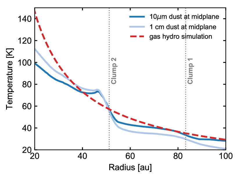
Figure 1: Azimuthally-averaged radial profile of the dust’s midplane temperature (solid curves) for the smallest (10 $\mu$m) and largest (1 cm) dust particles contributing to the (sub)millimetre continuum synthetic maps, and radial profile of the gas temperature in the hydrodynamical simulation (dashed curve). The dotted lines mark the location of Clumps 1 and 2.

2.2.2 Near-infrared polarised scattered light

Near-infrared polarised scattered light traces (sub)micron-sized grains at the surface of the disc, which are not included in our hydrodynamical simulations. To produce scattered light predictions, we include 12 bins of small grains ranging from 0.01 $\mu$m to 0.3 $\mu$m, and having the same density distribution and scale height as the gas in the simulations (these small grains are expected to be well coupled to the gas in our disc model). We artificially truncate the dust density within 0$\aas@@fstack{\prime\prime}$15 ($\sim$24 au) to avoid a strong contribution of the disc’s inner parts to the polarised intensity, which is not observed (Benisty et al., 2015). We also reduce the dust density beyond 0$\aas@@fstack{\prime\prime}$35 ($\sim$56 au, by a factor $\propto r^{-2}$) to decrease the scattering off dust grains outside the inner edge of the outer planet’s gap. The outer reduction is meant to mimic shadowing effects due to the gas spirals propagating between the two planets.

We further assume that the small grains are compact monomers forming a mixture of $60\%$ silicate and $40\%$ amorphous carbon, with an equivalent internal density of 2.7 g cm^-3. The optical constants for amorphous carbons are taken from Li & Greenberg (1997). The grains have a size distribution $n(s)\propto s^{-3.5}$, and their total mass is $\sim$$1.6\times 10^{-5}\rm M_{\star}$ (or $\sim$8 $M_{\oplus}$) in the results of Section 3. The grid used to compute the polarised scattered light images covers 5 pressure scale heights on both sides of the disc midplane with 30 cells evenly-spaced in colatitude.

To obtain the synthetic images of polarised scattered light, the dust temperatures are first computed with a thermal Monte Carlo calculation. We then compute the emergent Stokes maps $Q$ and $U$ at 1.04 $\mu$m ($Y$-band), which represent linear polarised intensities. Scattering is assumed to be anisotropic, and a full treatment of polarisation is adopted using the scattering matrix as implemented in RADMC3D. When included, white noise is added to the Stokes maps by adding at each pixel of the maps random numbers that have Gaussian probability distributions with zero mean and a standard deviation of 0.4% the maximum value of each map. This value is found to give a level of noise in the final convolved image of polarised scattered light that is close to that in the $Y$-band polarised intensity observation of Benisty et al. (2015), which we will compare our synthetic images to. A mask of $0\aas@@fstack{\prime\prime}2$ in radius is further applied to the Stokes maps so as to enhance the brightness of the spirals. The Stokes maps are then convolved with a circular beam of FWHM $0\aas@@fstack{\prime\prime}026$, which corresponds to the angular resolution achieved in Benisty et al. (2015). Next, the convolved Stokes maps are post-processed to obtain the local Stokes $Q_{\phi}$ following the procedure described in Avenhaus et al. (2017). Each pixel of the $Q_{\phi}$ synthetic image is finally scaled with the square of the deprojected distance from the central star in order to compare with the SPHERE image of Benisty et al. (2015).

3 Results

We present in this section the results of our hydrodynamical simulation, starting in Section 3.1 with the time evolution of the gas surface density and of the dust’s spatial distribution in response to the two planets. We show that the planets form dust-trapping vortices at the edges of their gap as a result of the RWI. Vortices may not be long-lived structures, however, and dust particles can progressively lose the azimuthal trapping of their vortex when the latter decays on account of the disc’s turbulent viscosity. Based on the ALMA and VLA continuum observations of Dong et al. (2018) and Casassus et al. (2019), which are displayed in the right-hand panels of Figs. 4 and 5, we argue that Clump 1 is consistent with azimuthal trapping in a vortex, while Clump 2 is more consistent with loss of azimuthal trapping in a decaying vortex. This is what we show in Section 3.2, where we compare our (sub)millimetre continuum synthetic maps with the observations. We then show in Section 3.3 that the two main spirals in the SPHERE image of Benisty et al. (2015), which is displayed in the right panel of Fig. 6, can be reproduced by two of the spiral waves induced by the outer planet in our disc model. Our synthetic maps have a fair number of free parameters, and our aim here is not to find a set of parameters that would fit the observations, but rather show that the two-vortex/two-planet scenario can indeed reproduce the most salient features in the MWC 758 disc.

3.1 Gas and dust evolutions

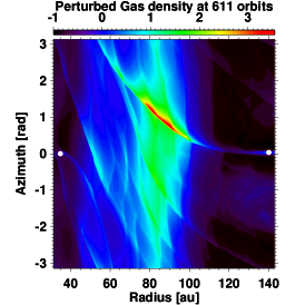
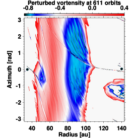
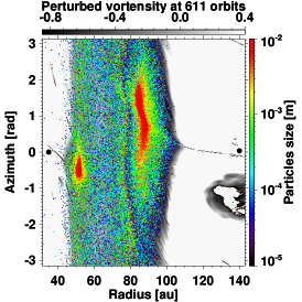
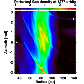
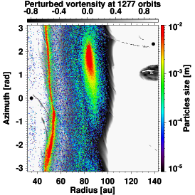
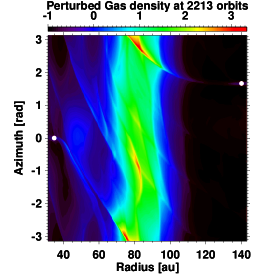
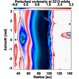
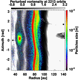
Figure 2: Gas structure and dust spatial distribution in the disc region between the planets. Results are shown in polar cylindrical coordinates at 611, 1277 and 2213 orbits from top to bottom. Left: perturbed gas surface density relative to its initial profile, $(\Sigma-\Sigma_{0})/\Sigma_{0}$. Middle: perturbed gas vortensity relative to its initial profile, ($\omega-\omega_{0})/\omega_{0}$. The color scale has been adjusted to highlight the large-scale azimuthal minima of vortensity, which trace the gas vortices. Right: same as the middle panels, but with a sequential colormap for the contours of perturbed vortensity, and with the location of the dust particles overlaid by coloured dots. The color bar on the right-hand side shows dust size in metres. In each panel, the filled circles at 35 au and 140 au mark the position of the planets.

3.1.1 Gaps, spirals and vortices in the gas

The planets in our disc model progressively carve a gap in the gas around their orbit. This is illustrated in the left panels of Fig. 2, which display the perturbed gas surface density relative to its initial radial profile, $(\Sigma-\Sigma_{0})/\Sigma_{0}$, at 611, 1277 and 2213 orbits after the beginning of the simulation (which is about 0.10, 0.22 and 0.38 Myr after the planets have reached their final mass). Results are shown in polar coordinates with the radius range ($x-$axis) narrowed to highlight the disc structure between the planets. The white circles spot the position of the planets. At 2213 orbits (near the end of the simulation), the azimuthally-averaged surface density of the gas has decreased by about $70\%$ of its initial value at the bottom of the inner planet’s gap, and by about $95\%$ at the bottom of the outer planet’s gap. The inner edge of the gap carved by the outer planet in the disc gas, which is at $\sim$90 au, is consistent with the truncation radius of the C¹⁸O ring in Boehler et al. (2018)’s ALMA band 7 data (see their Figure 4). The left panels of Fig. 2 also show multiple spiral arms in the disc gas, with some spirals more prominent than others. It is not straightforward to tell from these panels where each spiral originates, since spirals are triggered by the planets and the gas vortices that form in the disc. It is actually not straightforward either to tell where the vortices are, since the gas density perturbation in the spirals is as large, if not larger, than that in the vortices located between the planets.

The presence of gas vortices is more easily seen in the middle panels of Fig. 2, which display the perturbation of the gas vortensity¹ relative to its initial profile (the quantity $\{\omega-\omega_{0}\}/\omega_{0}$). Anticyclonic vortices show up as local minima in the gas perturbed vortensity in both the radial and azimuthal directions. A large-scale vortex is clearly visible at the inner edge of the outer planet’s gap (near 85 au) at 611 and 1277 orbits. It is, however, no longer active at 2213 orbits, which can be seen by the fact that the vortensity minimum at this location has turned axisymmetric (based on the gas vortensity, we estimate the lifetime of this vortex to be about 1800 orbits). The fact that the outer planet forms a vortex at the inner edge of its gap via the RWI is the consequence of the rather large planet’s mass, which initially allows the persistence of a radial pressure bump (or vortensity minimum) at this location notwithstanding the local turbulent viscosity (Bae et al., 2016). We have checked with a dedicated simulation that a very similar vortex structure forms in the absence of the inner planet.

The vortensity panels in Fig. 2 also show a vortex around the L5 Lagrange point located behind the outer planet in azimuth (at 140 au). Although not shown in Fig. 2, another vortex is situated at the outer edge of the outer planet’s gap near 230 au. There is no indication for vortices at both these locations in the (sub)millimetre observations of MWC 758, but it could be that the amount of dust trapped there is too small to have a measurable effect on the continuum emission.

A vortex also forms at the outer edge of the inner planet’s gap, near 50 au. This vortex has a rather unusual time evolution: it is active during the first 1000 orbits, it then decays and becomes inactive over the next 500 orbits, and finally builds up again and remains active for at least 700 more orbits (until the end of the simulation). This can be seen in the second column of panels in Fig. 2 by the presence at 611 and 2213 orbits of an azimuthal minimum in the gas perturbed vortensity at $\sim$50 au that is absent at 1277 orbits. The vortex decay coincides with a moderate increase in the eccentricity of the disc gas between the planets. This can be noticed by looking at the contours of perturbed vortensity. For instance, the vortensity maximum that is located around 60 au at 611 orbits is associated with gas on non-circular trajectories at 1277 orbits, with an eccentricity close to 0.1. This point will be further emphasized when describing the dust’s spatial distribution in Section 3.1.2.

The gas between the planets retains some level of eccentricity until the end of the simulation, yet the vortex forms again near 50 au from $\sim$1500 orbits. A possible explanation is the progressive increase in the vortensity maximum around 60 au, due to the eccentric motion of the gas and repeated interactions with the shock wakes of the planets. This evolution makes the vortensity minimum at the outer edge of the inner planet’s gap increasingly pronounced, which ultimately allows the RWI to set in again and form a vortex at this location. It does not affect the vortensity near the inner edge of the outer planet’s gap, however, and the vortex initially formed at this location progressively decays on account of the gas turbulent viscosity. Vortex decay will be further discussed in Section 4.2.

The reason why the disc gas between the planets becomes moderately eccentric is not clear. The growth of a global eccentric mode with azimuthal wavenumber $m=1$ has been observed in some simulations of massive self-gravitating discs (e.g., Pierens & Lin, 2018; Pérez et al., 2019), however, our Toomre Q parameter seems too high to support this idea (furthermore, the increase in the gas eccentricity is confined to the disc parts between the planets, and is therefore not global). Another possibility is that disc-planet interactions could account for this local increase in the disc eccentricity. This proposal deserves a specific study, which is beyond the scope of this paper.

We finally discuss the aspect ratio $\chi$ of the vortices, which measures their elongation. A rough estimate of $\chi$ can be obtained by using contours of constant perturbed vortensity in the second column of panels in Fig. 2. For instance, at 611 orbits, the aspect ratio of the vortex near 85 au can be estimated by using the light blue contour which marks a relative perturbation of vortensity of about -0.76. In doing so, the vortex can be approximated as an ellipse that extends from about -1.5 to 2.5 rad in azimuth, and from about 80 to 100 au in radius, which corresponds to $\chi\sim 18$. Interestingly, similar aspect ratios can be estimated for the inner vortex at 611 orbits, and for the outer vortex at 1277 orbits. In the same vein, we have checked that similar values for the aspect ratio of the outer vortex can be obtained based on the raw fluxes of continuum emission at 0.9 and 9 mm at 1277 orbits (see also Section 3.2.2) as well as on the reconstructed dust’s surface density (by approximating the spatial distribution of aforementioned quantities as ellipses, and measuring their aspect ratio).

3.1.2 Dust trapping in the vortices

The third column of panels in Fig. 2 displays the spatial distribution of the dust particles on top of the vortensity perturbation at 611, 1277 and 2213 orbits. The dust particles have a Stokes number ranging from about $10^{-5}$ to 0.1 in all the panels. The first thing to notice is that nearly all particles are confined between the planets, and more particularly along two rings. This is because the particles are inserted between the planets at 300 orbits after the beginning of the simulation, when the planets have already started to carve their gap. Particles thus tend to drift towards the inner edge of the outer planet’s gap, or towards the outer edge of the inner planet’s gap, since both locations are pressure maxima in the radial direction. We see that a few (mostly small) particles can cross the inner planet’s gap, which is due to the effect of dust turbulent diffusion kicking particles away from (and inside of) the gap’s edge.

The panels further illustrate the dust’s azimuthal trapping in the vortices. The top-right panel makes it clear that dust trapping correlates with minima in the gas vortensity rather than with maxima in the gas surface density. We also notice in this panel that the large particles trapped in the outer vortex get deflected inwards upon crossing the primary wake induced by the outer planet. We will come back to this effect in Section 4.3.1.

In the middle-right panel at 1277 orbits, we see that dust is still trapped in the outer vortex, that it is slightly eccentric, and that the azimuth at which these particles are trapped varies continuously with increasing particles size. By comparison, it is quite clear that the dust particles at the outer edge of the inner planet’s gap have lost azimuthal trapping as the inner vortex has decayed. They form a narrow eccentric ring, and from the orbital radius of the largest, cm-sized particles, which range from about 45 to 55 au, we infer a local eccentricity $\approx$0.1, very similar to that of the background gas (see Section 3.1.1). This eccentricity is consistent with that of the inner ring passing by Clump 2 in the ALMA observation of Dong et al. (2018) (see also Section 3.2). This dust ring is not axisymmetric, which reflects the fact that particles progressively lose memory of their former azimuthal trapping on different timescales depending on their size, much like in the simulations carried out in Fuente et al. (2017) to account for recent submillimetre observations of the AB Aurigae disc. We also note the presence of a faint eccentric ring of $\lesssim 1$ mm dust particles slightly interior to Clump 1, between $\sim$70 and 80 au, which is reminiscent to the ring of emission at $\sim$0$\aas@@fstack{\prime\prime}$43 seen in the ALMA observation of Dong et al. (2018). Comparison with Fig. 7 (Section 4.3.1) suggests that this ring could be due in part to deflections by the inner wake of the outer planet.

In the bottom-right panel of Fig. 2, at 2213 orbits, the inner vortex is formed again and it efficiently traps the dust at the outer edge of the inner planet’s gap. The outer vortex is now decayed, and the dust that was trapped at the outer vortex progressively acquires a near axisymmetric spatial distribution. This redistribution is not similar to that of the dust in the inner vortex when the latter had decayed. The dust leaving the outer vortex shifts radially inwards at a rate that depends on dust size. This shift, which arises because of repeated deflections upon crossing the inner wake of the outer planet, will be further described in Section 4.3.1.

Anticipating the results of the radiative transfer calculations in Section 3.2, we find that the faint emission of the inner ring passing by Clump 2 in the VLA observation of Casassus et al. (2019) cannot be accounted for by a compact dust distribution such as the one obtained in the early and late stages of our hydrodynamical simulation when the inner vortex is active. When the inner vortex is active, we find that the predicted peak intensity at 9 mm is indeed 1.5-2 times larger at Clump 2 than at Clump 1, while the observed ratio is $\sim$0.4 (see Section 3.2.1). We thus need the inner vortex to have decayed for the dust trapped at the outer edge of the inner planet’s gap to be distributed along an eccentric ring, and yet have a non-axisymmetric distribution. This is precisely the kind of distribution that the dust has in our simulations between $\sim$1000 and 1500 orbits, and which we have illustrated at 1277 orbits in the middle row of panels in Fig. 2.

We actually found a fair number of outputs in our simulation between 1000 and 1500 orbits that could account for the main observational features of the continuum maps at 0.9 mm (eccentric inner ring passing by Clump 2 with Clump 2 near pericentre, compact emission at Clump 1, azimuthal shift of about 130^∘ between Clumps 1 and 2) and at 9 mm (compact emission at Clump 1, faint emission at Clump 2). Out of these outputs, the one that best reproduces the observed maps is that at 1277 orbits.

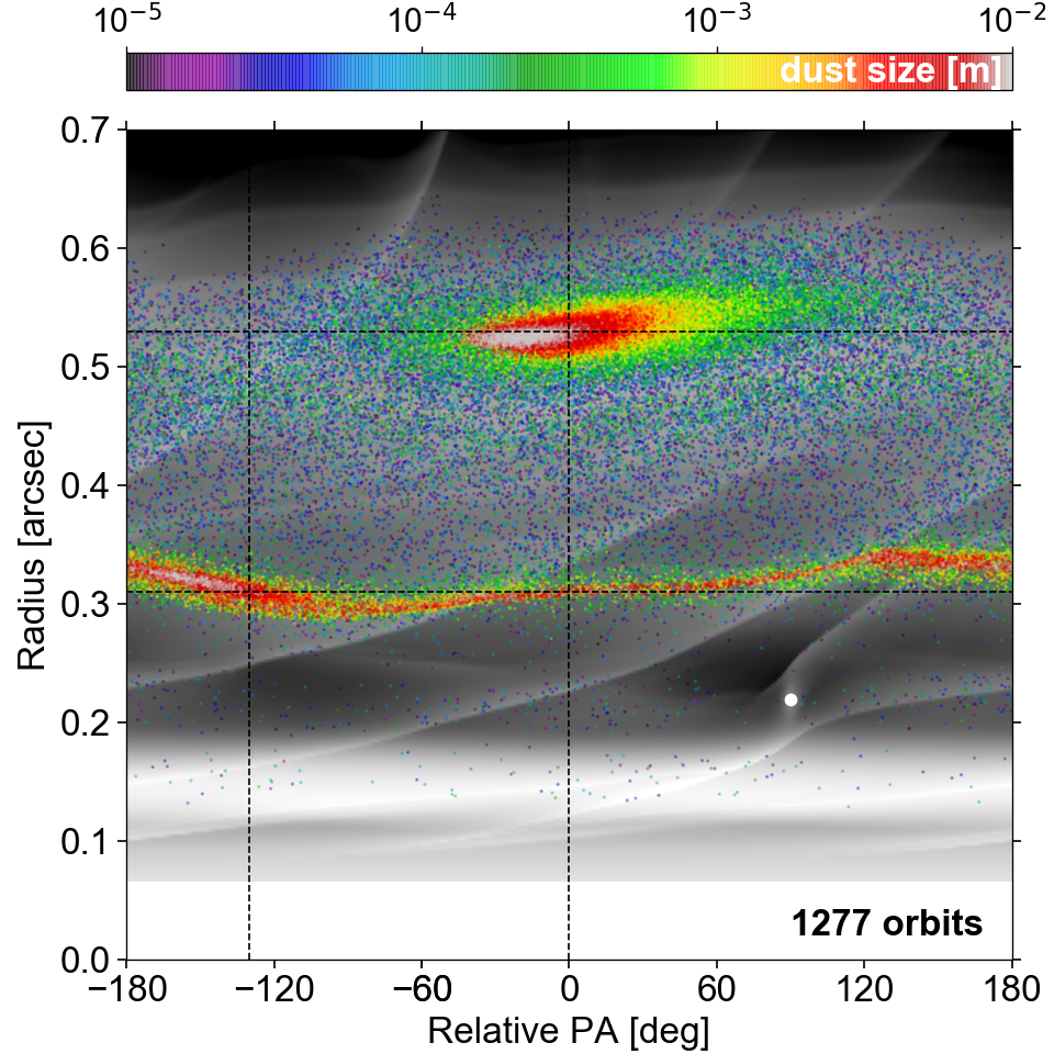
Figure 3: Gas surface density and dust spatial distribution in the hydrodynamical simulation at 1277 orbits ($\sim$0.2 Myr). The gas surface density is shown by black and white contours with a logarithmic colour scale (density increases from 0.1 to 10 g cm^-2 from black to white). The location of the dust particles is marked by coloured dots (colour varies with dust size, see colour bar on top of the image), and that of the inner planet by a white circle. Results are displayed in the disc plane, with the $y$-axis indicating distance from the central star in arcseconds (assuming a disc distance of 160 pc), and the $x$-axis the position angle (or azimuth) relative to the approximate location of the largest particles in the outer vortex. The image has been flipped horizontally to reflect that the disc is rotating clockwise in the observations, but counter-clockwise in the simulation. The dashed lines show the radius and position angle of the two clumps of emission in the deprojected ALMA continuum image of Fig. 4.

We finish this section by describing Fig. 3, which depicts again the dust’s spatial distribution at 1277 orbits, but now on top of the gas surface density in log scale. Results are displayed in polar coordinates, with the orbital radius in arcseconds in $y$-axis, and the azimuth (or position angle) relative to the approximate location of the largest particles in the outer vortex in $x$-axis. The inner planet is visible at $x=90^{\circ}$, $y\sim$ 0$\aas@@fstack{\prime\prime}$22. The figure is meant to be compared with the deprojected synthetic images of the (sub)millimetre continuum emission and of the near-infrared scattered light shown in Figs. 4, 5 and 6. It helps to understand how the dust particles in the simulation contribute to the (sub)millimetre continuum synthetic maps, which are most sensitive to the largest (mm- to cm-sized) particles that lie near the midplane. It also helps to see how the spiral density waves in the gas contribute to the polarised intensity image.

3.2 Continuum emission in the (sub)millimetre

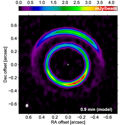
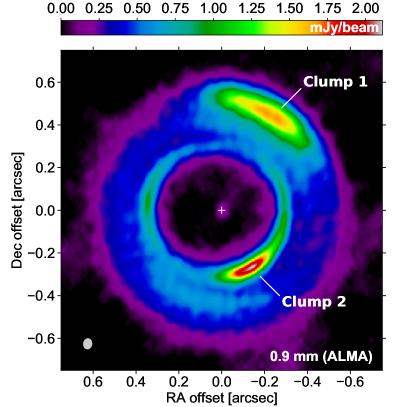
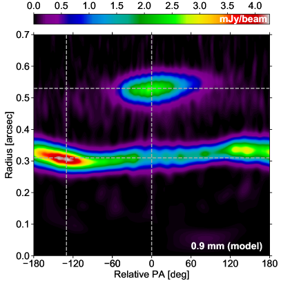
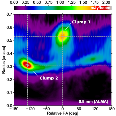
Figure 4: Predicted continuum emission at 0.9 mm with white noise (left panels) compared with the ALMA band 7 observation of Dong et al. (2018, right panels, images in natural weights). Upper panels: projected maps. The $x$- and $y$-axes indicate the offset from the stellar position in the right ascension (RA) and declination (Dec) in arcseconds, i.e., north is up and east is to the left. The beam ($0\aas@@fstack{\prime\prime}052\times 0\aas@@fstack{\prime\prime}042$ PA -7.1^∘) is shown by the ellipse in the bottom-left corner in each panel, and the star by a plus symbol. Lower panels: deprojected maps (assuming a disc inclination of $21^{\circ}$ and a position angle of $62^{\circ}$). The $y$-axis shows orbital radius in arcseconds, the $x$-axis the position angle in degrees relative to that of Clump 1. The dashed curves mark the position angle (relative to Clump 1) and orbital radius of each clump in the ALMA image.

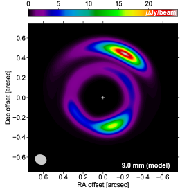
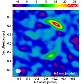
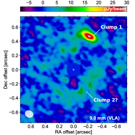
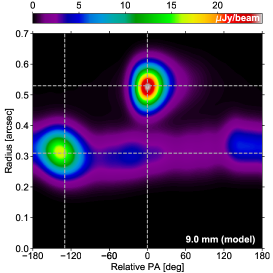
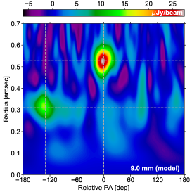
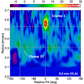
Figure 5: Predicted continuum emission at 9 mm without and with white noise (left and middle panels, respectively) compared with the VLA observation of Casassus et al. (2019, right panels). The star has been subtracted in the VLA images. Upper panels: projected maps (as in the upper panels of Fig. 4). The beam ($0\aas@@fstack{\prime\prime}12\times 0\aas@@fstack{\prime\prime}10$ PA 65^∘) is shown by the ellipse in the bottom-left corner in each panel, and the star by a plus symbol. Lower panels: deprojected maps (as in the lower panels of Fig. 4). The dashed curves mark the position angle (relative to Clump 1) and orbital radius of each clump in the ALMA image shown in Fig. 4.

A side-by-side comparison of our synthetic maps of continuum emission with the ALMA image of Dong et al. (2018, $\lambda\approx 0.9$ mm) and the VLA image of Casassus et al. (2019, $\lambda\approx 9$ mm) is displayed in Figs. 4 and 5, respectively. In each figure, the projected maps (flux maps in the sky plane) are in the upper panels, and the deprojected maps (flux maps in the disc plane) are in the lower panels. Fig. 4 shows only the synthetic map at 0.9 mm with white noise since its amplitude is very small (the predicted peak intensity at Clump 2 is $\sim$200 times larger than the rms noise level). Fig. 5, however, displays the synthetic map at 9 mm without and with white noise since the predicted peak intensity at Clump 1 is only $\sim$12 times the rms noise level. For comparison with our synthetic maps at 9 mm, the star has been subtracted in the VLA images shown in the right column of panels in Fig. 5. We point out that the noise in the VLA observation includes smaller scales than our synthetic map with white noise. This is most likely due to the core of the VLA dirty beam not being perfectly represented by an elliptical Gaussian.

Overall, for the assumed dust properties, our two-vortex model captures the main features of the two clumps of emission observed in the ALMA and VLA images. The dust-trapping vortex at the inner edge of the outer planet’s gap can reproduce the compact emission associated with Clump 1 (at $\sim$1 o’clock in both the ALMA and VLA images). In particular, we recover the fact that Clump 1 is azimuthally broader at 0.9 mm than at 9 mm, as expected with azimuthal dust trapping. The decaying vortex at the outer edge of the inner planet’s gap reproduces well the eccentric inner ring passing by Clump 2, with Clump 2 near pericentre (at $\sim$5 o’clock in the ALMA image). It also forms a secondary clump of emission near apocentre which could account for the emission seen to the east of the ring in the ALMA image (at $\sim$9 o’clock). And importantly, we recover the more diffuse and rather low level of emission seen in the VLA image for Clump 2. By comparing the synthetic deprojected maps in Figs. 4 and 5 with Fig. 3, it is easy to see that the location of the maxima in the synthetic maps corresponds to that of the largest dust particles in the simulation (those ranging from a few mm to a cm in size).

Comparison between the synthetic and observed flux maps at 0.9 mm further indicates that Clump 1 and Clump 2 lie on top of a fainter ring of background emission. This background emission could trace a rather massive population of small dust well coupled to the gas. This idea will be presented in Section 4.3.5 and illustrated in Fig. 8. We also note the presence in our synthetic map at 0.9 mm of a faint ring of emission slightly interior to Clump 1, at a level of emission ($\sim$0.1 mJy/beam) that is close to the rms noise level adopted in the synthetic map. This faint ring of emission traces the dust ring situated between 0$\aas@@fstack{\prime\prime}$44 and 0$\aas@@fstack{\prime\prime}$50 in Fig. 3 (or, equivalently, between $\sim$70 and 80 au in the middle-right panel of Fig. 2). As already stated in Section 3.1.2, this ring is reminiscent to the ring of emission around 0$\aas@@fstack{\prime\prime}$43 in the ALMA observation of Dong et al. (2018), and which peaks at about 0.6 mJy/beam in the right panels of Fig. 4.

We also briefly comment that the inclusion of anisotropic scattering in the radiative transfer calculations has a minor impact on our (sub)millimetre continuum synthetic maps. At 0.9 mm, anisotropic scattering increases the overall level of flux by only a few percent compared to a radiative transfer calculation that only includes thermal absorption. At 9 mm, anisotropic scattering increases the overall level of flux by about 20%.

In the following, we provide a more quantitative comparison between our predictions and the observations, in terms of the peak intensities, and the widths and aspect ratio of Clump 1. We also quote the peak absorption optical depths in the synthetic maps.

3.2.1 Peak intensities

At Clump 1, the predicted peak intensity at 0.9 mm is $\sim$2.6 mJy/beam, which is $\sim$50% larger than the observed value, while the predicted peak intensity at 9 mm is $\sim$24.8 $\mu$Jy/beam (without noise), which is close to the observed value of $29.1\pm 2.0$ $\mu$Jy/beam. At Clump 2, the predicted peak intensity at 0.9 mm is $\sim$4.2 mJy/beam (about twice the observed value), that at 9 mm is $\sim$17.0 $\mu$Jy/beam (without noise), which is $\sim$1.6 times larger than the observed value of $10.8\pm 2.0$ $\mu$Jy/beam. Our model thus tends to produce a little too much flux at Clump 2, although a direct comparison is not trivial because of different shapes and emitting areas for Clump 2 in the predictions and the observations.

The predicted peak intensity ratio between Clump 1 and Clump 2 is about 0.6 at 0.9 mm and 1.4 at 9 mm, while the observed values are about 0.8 at 0.9 mm and 2.7 $\pm$ 0.3 at 9 mm. We interpret the larger peak intensity ratio at 9 mm as a consequence of the vortex decay that leads to Clump 2 in our model. We have checked this by computing synthetic flux maps at 611 orbits, when the inner vortex is still active (see top panels in Fig. 2), which show that the peak intensity ratio takes very similar values at both wavelengths (it is about 0.5 at 0.9 mm, and 0.6 at 9 mm).

We point out that in the ALMA band 7 observations of Boehler et al. (2018), for which the angular resolution is about twice as large as in the ALMA band 7 observations of Dong et al. (2018), Clump 1 has a larger peak intensity than Clump 2. The peak intensity ratio between Clump 1 and Clump 2 is about 1.6 in Boehler et al. (2018), while it is about 0.8 in Dong et al. (2018). By convolving our raw flux maps with the same beam as Boehler et al. (2018)’s observations ($0\aas@@fstack{\prime\prime}11\times 0\aas@@fstack{\prime\prime}08$ PA 38^∘), we find a peak intensity ratio between Clump 1 and Clump 2 of $\sim$0.85, thus larger than the value of $\sim$0.6 that we get with the same resolution as in Dong et al. (2018), but still smaller than 1. Our model cannot reproduce the reversal in the peak intensity ratio between both aforementioned angular resolutions.

We finally note that Clump 1 is offset by about 0$\aas@@fstack{\prime\prime}$03 in the ALMA and VLA images, which is not reproduced in our models. On the contrary, there is no significant azimuthal shift between the positions of Clump 1 in the ALMA and VLA images, whereas the synthetic images show an azimuthal shift by about 10^∘, with the peak at 9 mm shifted clockwise (in the direction opposite to that of rotation). A very similar azimuthal shift is actually predicted for Clump 2. We stress that this azimuthal shift is not a systematic prediction of our models: at some other outputs in the simulation, the azimuthal shift is in the opposite direction (shift by $\sim$-10^∘), while at some other outputs we find no azimuthal shift. The predicted azimuthal shift is likely related to Clump 1’s eccentricity.

3.2.2 Widths and aspect ratio of Clump 1

From the polar maps displayed in Fig. 4 and 5, we see that Clump 1 tends to have a slightly larger azimuthal width and smaller radial width in the synthetic maps than in the observations. In the azimuthal direction, the predicted FWHM of the convolved intensity across the peak is about 45^∘ and 19^∘ at 0.9 mm and 9 mm, respectively, while the observed values are about 28^∘ and 12^∘. Similarly, in the radial direction, the predicted FWHM of the convolved intensity across the peak is about 0$\aas@@fstack{\prime\prime}$04 and 0$\aas@@fstack{\prime\prime}$05 at 0.9 mm and 9 mm, respectively, while the observed values are about 0$\aas@@fstack{\prime\prime}$08 and 0$\aas@@fstack{\prime\prime}$06. A similar analysis can be done for Clump 2, with the same conclusion that, in our model, Clump 2 tends to be a little narrower in radius and somewhat broader in azimuth than in the ALMA observation of Dong et al. (2018). Fine tuning of the disc gas parameters (surface density, temperature, alpha viscosity) and of the dust parameters (size distribution, mass, internal density) could potentially reconcile our predictions and the data. A full parameter search is beyond the scope of this work.

Moreover, from the radial and azimuthal widths of Clump 1 in the emission maps, and the radial location of the peak intensity, we can estimate again the aspect ratio $\chi$ for Clump 1. We find that the predicted $\chi$ values amount to $\sim$10.2 and $\sim$3.5 at 0.9 mm and 9 mm, respectively, while the observed values are $\sim$3.2 and $\sim$1.8 (with about 10% relative uncertainties). These values are much smaller than the one obtained via the gas perturbed vortensity in the vortex from which Clump 1 originates (see last paragraph in Section 3.1.1). We have checked that this discrepancy comes about because of the beam convolution. Upon calculating the synthetic maps of raw intensity (intensity of continuum emission prior to beam convolution), we obtain $\chi\approx 16\pm 2$ at both wavelengths, which agrees well with the vortex’s aspect ratio measured via the gas vortensity, and also with the value reported in Casassus et al. (2019) where steady-state dust trapping predictions based on Lyra & Lin (2013) are used to model the raw intensity for Clump 1 at 0.9 and 9 mm.

3.2.3 Peak optical depths in absorption

An interesting information that is accessible with our synthetic maps of continuum emission is the absorption optical depth that our model predicts at the location of the peak intensities. At 0.9 mm, we find maxima in the absorption optical depth of about 30 and 15 for Clump 1 and Clump 2, respectively. The continuum emission at 0.9 mm is therefore very optically thick near the centre of both clumps. At 9 mm, the absorption optical depth peaks at about 0.9 and 0.4 for Clump 1 and Clump 2, respectively, which are perhaps surprisingly large values at this wavelength. The peak absorption optical depth at 9 mm near the centre of Clump 1 is a bit larger than the value of $\sim$0.3 predicted by the steady-state dust trapping predictions used in Casassus et al. (2019), but note that the gas vortex and dust distribution assumed to give rise to Clump 1 in Casassus et al. (2019) have different physical parameters than in our simulation (different alpha turbulent viscosity, temperature, dust’s internal density and opacity; see Section 3.3.2 in Casassus et al., 2019 for comparison).

3.3 Polarised scattered light in $Y$-band

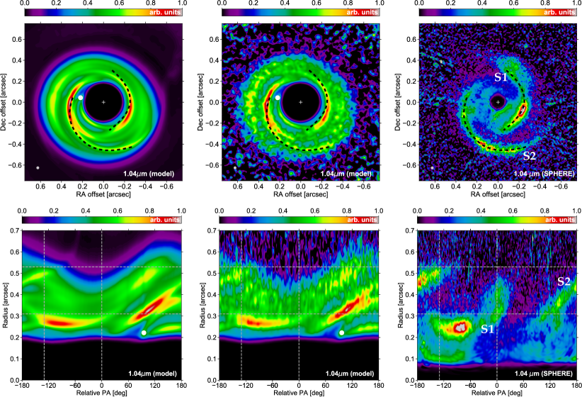
Figure 6: Synthetic scattered light image at 1.04 $\mu$m without and with noise (left and middle panels, respectively) compared with the $Y$-band SPHERE image of Benisty et al. (2015, right panels). In each image, the polarised intensity is scaled by the square of the deprojected distance from the central star, and normalised such that the intensity of the strongest pixel is 1. To highlight the spirals structure, a mask of 0$\aas@@fstack{\prime\prime}$2 radius is applied to the synthetic images. Upper panels: projected maps (as in the upper panels of Fig. 4). The beam ($0\aas@@fstack{\prime\prime}026\times 0\aas@@fstack{\prime\prime}026$) is shown by the ellipse in the bottom-left corner in each panel, the star by a plus symbol, and the inner planet by a white circle. The outer planet is outside the image domain (at 0$\aas@@fstack{\prime\prime}$87, PA -60^∘). The dashed curves in all three panels are used to compare the synthetic and observed asymmetries, but they are not fits to the observed spiral traces. Lower panels: deprojected maps (as in the lower panels of Fig. 4). The position of the inner planet is marked by a white circle in the synthetic images. The dashed curves mark the position angle (relative to Clump 1) and orbital radius of each clump in the ALMA image shown in Fig. 4.

A side-by-side comparison between our synthetic map of polarised scattered light with the $Y$-band ($\lambda=1.04$ $\mu$m) scattered light image of Benisty et al. (2015) is displayed in Fig. 6. The projected maps are in the upper panels, and the deprojected maps in the lower panels. The synthetic maps in the first column of panels do not include noise, those in the second column include white noise with the method described in Section 2.2.2. All images are multiplied by the square of the deprojected distance from the central star, and normalised such that the intensity of the strongest pixel is 1. To highlight the asymmetric structures in our synthetic map, a mask of $0\aas@@fstack{\prime\prime}2$ radius is applied. Recall that the dust density within 0$\aas@@fstack{\prime\prime}$15 has been truncated, and that beyond 0$\aas@@fstack{\prime\prime}$35 has been reduced (see Section 2.2.2). The same dashed curves are superimposed in the upper panels to compare the predicted and observed asymmetries; however, we stress that they are not fits to the observed spiral-like features – they are just drawn to guide the eye.

Overall, we see that our model predicts several spiral arms, but two are more prominent. Just like the spirals in the gas surface density of the simulation (see Figs. 2 and 3), the spirals in the synthetic scattered light image do not all have a clear origin, as they trace spiral density waves due to either the planets, the vortices, or a combination thereof. Some insight into the origin of the spirals and/or asymmetries in the synthetic image can be gained by comparing the deprojected maps with the gas surface density contours in Fig. 3. Interestingly, we see that our synthetic map can reproduce both the location and the winding of the observed spiral arm to the south-east very well (see the dashed curve denoted by S2 in Fig. 6). According to our model, this spiral arm would be the (primary) inner wake of the outer planet, which propagates from the outer planet’s position. Our synthetic image shows a second prominent spiral to the west, which corresponds to a secondary spiral density wave induced by the outer planet. This spiral nearly coincides with the bright concentric arc to the west of the SPHERE image (see the lower part of the dashed curve denoted by S1 in Fig. 6). The same spiral is (mainly) responsible for the emission to the east of the synthetic map (near 9 o’clock beyond 0$\aas@@fstack{\prime\prime}$4), but this emission is not observed in the SPHERE image. The arc-shaped peak slightly inside of Clump 1 does not have a clear counterpart in our synthetic map.

The synthetic $Y$-band polarized light images in Dong et al. (2015) and Dong et al. (2018), which are obtained from 3D hydrodynamical simulations, had previously shown that the two inner wakes of a planet several times the mass of Jupiter could qualitatively account for the two spiral arms in the SPHERE image of MWC 758. Note, however, that the planet that they considered was located at $\sim$0$\aas@@fstack{\prime\prime}$6 (100 au), which is quite close to Clump 1 in the (sub)millimetre images ($\sim$85 au), and it seems difficult for such a massive planet to form a dust-trapping vortex at this short separation.

We finally stress that a realistic energy equation and three-dimensional effects, which are not taken into account in our hydrodynamical simulations, could well affect the way spirals would look like in polarised intensity images, in particular the appearance of the secondary wake induced by the outer planet (Zhu et al., 2015; Fung & Dong, 2015; Dong & Fung, 2017). For this reason we will not press the comparison between our synthetic polarised intensity image and the observed image too far. It could well be that the reproduction of the S2 spiral is actually coincidental.

4 Discussion and summary

4.1 Importance of gas self-gravity

The simulations carried out in this study include gas self-gravity, which might seem unnecessary since the (azimuthally-averaged) Toomre $Q$-parameter remains much larger than unity in our disc model. $Q$ reaches a local minimum of about 30 at the inner edge of the outer planet’s gap, near 85 au (Clump 1’s location). However, as shown in previous studies (Lin & Papaloizou, 2011; Lin, 2012; Lovelace & Hohlfeld, 2013; Zhu & Baruteau, 2016; Regály & Vorobyov, 2017), gas self-gravity significantly weakens large-scale RWI vortices (with azimuthal wavenumber $m=1$) when the product of $Q$ and $h$ becomes smaller than $\sim$$\pi/2$ at the vortex location. Given our uniform aspect ratio $h=0.088$, vortices become significantly impacted by self-gravity for $Q\lesssim 18$. Had we taken a larger initial surface density for the gas in our simulations, the vortex formed at $\sim$85 au would have been weaker and would have therefore decayed earlier. Said differently, with gas self-gravity included, a rather low surface density for the gas at the vortex location is necessary for the dust trap to match the high concentration of dust grains inside the vortex core, and consequently the compactness of Clump 1 seen in the ALMA and VLA observations. This rather low surface density is consistent with that estimated by Boehler et al. (2018) based on ALMA band 7 observations of ¹³CO and C¹⁸O.

4.2 Vortex decay

In this study, we present a scenario where the asymmetric eccentric ring and the compact crescent seen in the ALMA band 7 continuum data of the MWC 758 disc are due to planet-induced vortices. To explain the low and diffuse signal obtained with the VLA at the location of the ring, we propose that this ring results from a decaying vortex. In our simulations, vortex decay is mediated by viscous diffusion ($\alpha=10^{-4}$), and is found to coincide with a moderate increase in the gas eccentricity between the planets (see Section. 3.1.1). Notwithstanding this moderate eccentricity of order 0.1, the lifetime of the vortex that gives rise to the asymmetric ring, about a thousand orbits of the inner planet, is consistent with previous 2D simulations of planet-induced vortices for similar disc parameters and planet masses (e.g., Fu et al., 2014a). A smaller turbulent viscosity would increase the lifetime of the vortices in our simulations. However, as we have checked with preliminary simulations, it would also cause a higher concentration of the large dust particles in the vortices, and would therefore increase the compactness of the (sub)millimetre emission at both dust traps in a way that is not consistent with neither the ALMA nor the VLA observations. On the other hand, a larger turbulent viscosity would shorten the lifetime of the vortices, thereby making the dust’s azimuthal trapping scenario for Clump 1 less likely. Furthermore, several factors other than the disc’s turbulent viscosity affect the growth and decay timescales of planet-induced vortices in 2D viscous disc models, including the timescale for planetary growth (Hammer et al., 2017; Hammer et al., 2019), which is taken to be the same for both planets in our model, a non-isothermal energy equation (Les & Lin, 2015), gas self-gravity (Lin & Papaloizou, 2011), or dust feedback on the gas (Fu et al., 2014b).

About dust feedback, we stress that for the total mass and size distribution of the dust adopted in our radiative transfer calculations, the dust-to-gas mass ratio in the vortices that correspond to Clump 1 and Clump 2 does not exceed $\sim$0.1. This rather low value implies that dust feedback should have a small-to-moderate impact on the vortices if it were included in our hydrodynamical simulations (see, e.g., Crnkovic-Rubsamen et al., 2015, who showed that vortices could be destroyed for dust-to-gas mass ratios $\geq$ 0.3-0.5 within the vortices).

The level of viscosity adopted in our simulations is meant to model the effects of MHD turbulence in the outer regions of a protoplanetary disc, where non-ideal MHD effects, in particular ambipolar diffusion, should play an important role. Modelling turbulence as a diffusion process is uncertain when the typical length scale of interest (here, that of the gas vortex) is of the order of the pressure scale height. Zhu & Stone (2014) have investigated growth of and dust trapping in planet-induced vortices via global 3D MHD simulations. One of their simulations including ambipolar diffusion shows that the vortex formed at the outer edge of the gap carved by a 9 Jupiter-mass planet decays in about 1000 orbital timescales, with a similar lifetime found in a 2D hydrodynamical simulation using an equivalent turbulent viscosity. This result gives credit to the vortex’s decay timescales obtained in 2D viscous disc simulations.

MHD turbulence put aside, the growth and persistence of vortices in 3D disc models have been intensively examined over the last decade or so. We mention here a few results that are relevant to our study. Lesur & Papaloizou (2009) have found that anti-cyclonic vortices could be unstable against the elliptic instability, a parametric instability that mainly occurs at small scales, and which is stronger for vortices with small aspect ratios ($\chi\lesssim 4$). The global 3D simulations of Meheut et al. (2012) have shown that a vortex formed by the Rossby-Wave Instability developed meridional circulation and could survive over hundreds of dynamical timescales before decaying, most probably because of the elliptic instability. Regarding planet-induced vortices in 3D, the impact of gas self-gravity has been examined by Lin (2012), essentially recovering the predictions of 2D simulations, and the impact of a layered disc structure (through a viscosity increasing with height from the midplane) has been tackled by Lin (2014), who found that a high ($\alpha\sim 10^{-2}$) viscosity in the disc’s upper layers could largely decrease the vortex’s lifetime, despite a modest viscosity ($\alpha\sim 10^{-4}$) in the disc midplane. About gas self-gravity, we also highlight the recent work of Lin & Pierens (2018), who have shown with 3D shearing box simulations that gas self-gravity could prevent the decay of 3D vortices against elliptic instabilities, which would otherwise destroy them in non self-gravitating discs.

To our knowledge, the impact of the elliptic instability on the growth and survival of planet-induced vortices has not been investigated yet. This would probably require 3D global, vertically-stratified, high-resolution simulations of planet-disc interactions. It would also be of interest to examine how the elliptic instability behaves in the presence of other sources of turbulence, such as non-ideal MHD turbulence.

We finally discuss to what extent the proposed vortex decay scenario is associated with a transient phenomenon. To interpret the ALMA and VLA observations of MWC 758, the inner vortex is required to have decayed significantly (but with the dust retaining some degree of non-axisymmetry), while the outer vortex has not yet significantly decayed. Given the planets mass and disc parameters in our model, it takes $\sim$0.17 Myr after the planets have reached their final mass for the inner vortex to decay, and $\sim$0.30 Myr for the outer vortex. Both timescales look short in comparison to the estimated age of the system (5 to 10% of the age), and one may argue that we are catching the system at a special time. Interestingly, this ratio is actually consistent with the fraction of discs with (sub)millimetre continuum annular substructures that have high-contrast azimuthal asymmetries like in the MWC 758 disc (7 out of 43, or $\sim$16%; see Huang et al., 2018.) However, one should bear in mind that it takes time to grow the planets in the first place, and it is unclear how long it should take to form a 1.5 Jupiter-mass planet at 35 au and a 5 Jupiter-mass planet at 140 around an A5-type star. The lifetime of the vortices in our model is also uncertain, and it would be interesting to investigate how slow planetary growth, over a significant fraction of the disc age, would change our scenario, since it has been shown that slow growth tends to produce weaker vortices (Hammer et al., 2017; Hammer et al., 2019). Similarly, the planets in the simulation have been kept on circular orbits, and it is therefore relevant to explore how migration would affect the growth and survival of the vortices, and the eccentricity of the disc gas between the planets.

4.3 Impact of dust parameters

We discuss here how the size distribution, the total mass, the internal density and the opacities of the dust particles affect the results of our simulations and of our (sub)millimetre continuum synthetic maps (Sections 4.3.1 to 4.3.4). We then present in Section 4.3.5 (sub)millimetre continuum synthetic maps which include a population of small dust between the planets.

4.3.1 Dust’s size distribution

Throughout this work, we assume that the size of the dust particles follows a power-law distribution, with thus three parameters: the minimum and maximum sizes, and the power-law exponent. We recall that the results presented in Section 3.2 are for a size distribution $n(s)\propto s^{-3}$ for particles sizes $s$ between 10 $\mu$m and 1 cm. Decreasing the minimum size is found to have no impact on our synthetic maps in the (sub)millimetre, as particles smaller than 10 $\mu$m have a very small contribution to the continuum emission at both 0.9 mm and 9 mm. A notable exception will be presented in Section 4.3.5, where we relax the assumption of a power-law size distribution by adding a rather massive population of small dust.

The maximum size assumed for the dust particles has, however, a much higher impact on our results. To see why this is the case, we display in Fig. 7 the dust’s spatial distribution at 1277 orbits overlaid on the gas perturbed vortensity, just like in the middle-right panel of Fig. 2, except that we now show the location of dust particles up to 10 cm in size (instead of 1 cm). We see that particles larger than about 1.5 cm are not trapped in the vortex at $\sim$85 au, but are shifted radially inwards by about 5 to 10 au at this time in the simulation. This radial shift stems from the interaction between the large dust particles and the inner wake of the outer planet. Since this wake carries negative fluxes of energy and angular momentum, it pushes dust particles inwards each time they cross the wake. Fig. 7 shows that, at the vortex’s orbital radius, the radial deflection caused by the planet wake is larger than the radial drift back towards the vortex for dust particles larger than about 1 cm, which have a Stokes number $\gtrsim$ 0.1. These particles thus find an equilibrium location interior to the vortex, where they form a nearly axisymmetric ring. Investigation of dust-wake interactions and their observational implications for the continuum emission in the (sub)millimetre will also be detailed in a forthcoming paper (Baruteau et al., in prep.). For the present work dedicated to MWC 758, we have checked that this ring of $\gtrsim$ cm-sized dust particles would make the (sub)millimetre emission near Clump 1 much more extended in the azimuthal direction than predicted in Figs. 4 and 5 for the same total dust mass, which would be incompatible with the compactness of Clump 1 as observed by ALMA and especially the VLA. This could have interesting implications for dust growth in the MWC 758 disc, as our model suggests inefficient growth beyond cm sizes around the location of Clump 1, which we speculate might be due to bouncing and/or fragmentation barriers.

Lastly, we have checked that the slope of the dust’s size distribution has, overall, a mild impact on the predicted (sub)millimetre emission for Clump 1 and Clump 2. Qualitatively, we find that the shallower the size distribution, the more compact the emission is for Clump 1 at 0.9 mm as well as at 9 mm.

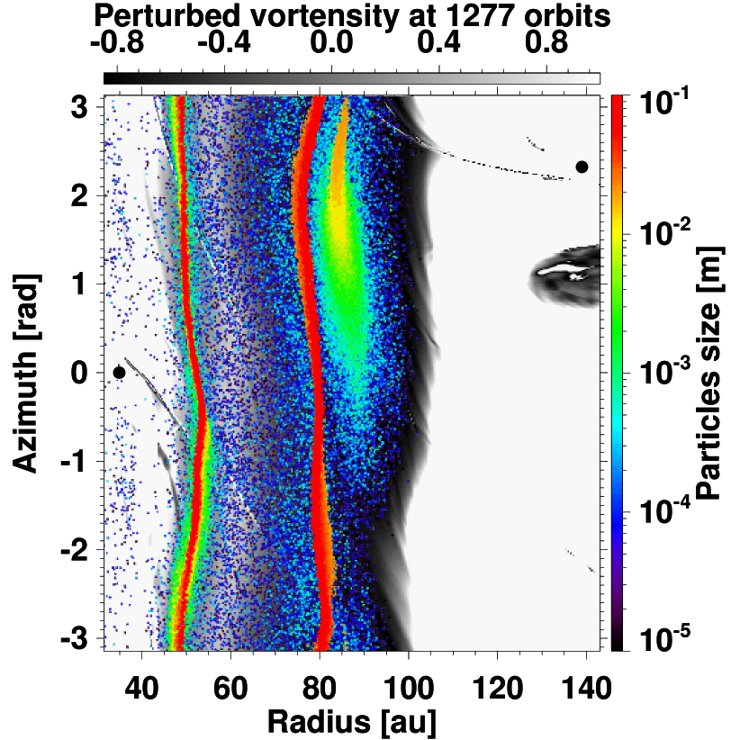
Figure 7: Same as middle-right panel of Fig. 2, but including dust particles between 1 cm and 10 cm in size.

4.3.2 Dust’s total mass

For the dust mass adopted in Section 3 ($1.6\times 10^{-4}M_{\star}$ between $\sim$40 au and $\sim$100 au), the peak absorption optical depth at 0.9 mm is $\sim$30 for Clump 1 and $\sim$15 for Clump 2 (see Section 3.2.3). We have checked that increasing the total dust mass would result in even larger absorption optical depths at both clumps, and thus more extended emissions in the azimuthal direction, which would be incompatible with the observed compactness of both clumps at 0.9 mm. Increasing the total dust mass too much would also conflict with the assumption that dust feedback has been discarded in the hydrodynamical simulation.

Decreasing the total dust mass would reduce the peak intensity of Clump 2 faster than for Clump 1, thereby increasing the peak intensity ratio between Clump 1 and Clump 2 at both wavelengths. For instance, by reducing the total dust mass used in Section 3 by a factor 2, the peak intensity ratio between Clump 1 and Clump 2 increases from about 0.6 to 0.7 at 0.9 mm (observed value is $\sim$0.8), and from about 1.4 to 1.7 at 9 mm (observed value is $\sim$2.7 $\pm$ 0.3). However, since the emission at 9 mm is only marginally optically thick at both clumps, decreasing the dust mass would also decrease the overall flux level, which would reduce the level of agreement between the predicted and observed peak intensities for Clump 1 at 9 mm. In the above example, halving the total dust mass reduces the predicted peak intensity for Clump 1 at 9 mm from $\sim$24.8 to $\sim$14.5 mJy/beam (observed value is 29.1 $\pm$ 2 mJy/beam).

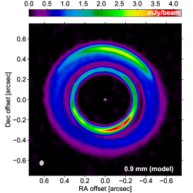
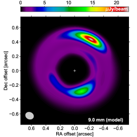
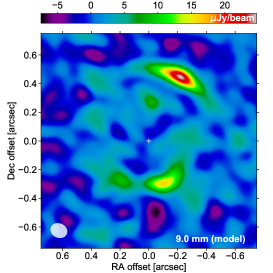
Figure 8: Synthetic maps of continuum emission at 0.9 mm (left panel) and at 9 mm (without and with white noise, middle and right panels) obtained by adding a rather massive ($\sim$24 $M_{\oplus}$) population of small dust well coupled to the gas between Clumps 1 and 2.

4.3.3 Dust’s internal density

The particles internal density adopted throughout this study, $\rho_{\rm int}=0.1$ g cm^-3, may seem a little surprising as simulations and/or radiative transfer calculations usually model dust as compact grains with an internal density of a few g cm^-3. During the course of this project, we carried out a simulation with a more conventional internal density of 1 g cm^-3, and obtained synthetic maps in the (sub)millimetre that have nearly the same morphology than for $\rho_{\rm int}=0.1$ g cm^-3 if the maximum particle size is set to 1 mm instead of 1 cm. This reduced maximum size comes about because the particles dynamics is primarily set by the Stokes number, which scales with the product of particles size and internal density. For $\rho_{\rm int}=1$ g cm^-3, particles larger than about 1 mm are shifted interior to the vortex located at $\sim$85 au because of the inner wake of the outer planet, just like the particles larger than about 1 cm in our simulation with $\rho_{\rm int}=0.1$ g cm^-3, as shown in Section 4.3.1.

The main difference between both internal densities is that, in the continuum emission at 0.9 mm, the peak intensity as well as the azimuthal width are a little larger at $\rho_{\rm int}=1$ g cm^-3 for both clumps, but probably a similar level of agreement could be attained by fine tuning the other parameters for the dust. Our results therefore cannot rule out that the dust in the MWC 758 disc could be compact, given the degeneracy in the predictions, and the large uncertainties in the dust opacities (at either internal density, actually). It would be interesting to explore the possibility of even smaller internal densities (see, e.g., Kataoka et al., 2013).

4.3.4 Dust opacities

The dust composition is another free parameter that we have tested for the (sub)millimetre continuum synthetic maps. The dust composition only impacts the calculation of the dust absorption and scattering opacities. Recall that all the results in Section 3 are obtained for porous dust particles for which the solid component comprises 70% water ices and 30% silicates. By testing a different mixture, namely 70% silicates and 30% amorphous carbons, we find that the overall level of flux at 0.9 mm is reduced by only $\sim$15%, and that at 9 mm by a factor $\sim$3. Again, given the degeneracy of the predictions, we would find it difficult to constrain the dust composition from the comparison between the synthetic maps of continuum emission and the observations.

4.3.5 Inclusion of small dust

The synthetic and observed flux maps at 0.9 mm shown in Fig. 4 indicate that Clump 1 and Clump 2 lie on top of a fainter ring of background emission. As alluded to in Section 3.2, this emission might come about because of small dust forming as a result of dust fragmentation between the planets. The spiral shocks and the (moderately) eccentric gas between the planets in our disc model (Section 3.1.1) a priori offer an environment ripe for dust fragmentation. Since dust growth and fragmentation are not implemented in our hydrodynamical code, we have tested this idea by simply adding an extra bin of small dust in our radiative transfer calculations. Since the absorption and scattering opacities of our porous dust is largely independent of dust sizes below 10 $\mu$m, we need not specify what size range this extra bin of small dust precisely corresponds to. We will just assume these dust particles remain larger than 0.3 $\mu$m, to distinguish them from the compact dust particles that contribute to the near-infrared polarised scattered light (Section 2.2.2).

The extra bin of small dust that is added to our synthetic maps of continuum emission is assumed to have a spatial distribution that follows that of the gas between 0$\aas@@fstack{\prime\prime}$4 and 0$\aas@@fstack{\prime\prime}$6, and a total mass $\sim$0.6% the mass of the gas (or 24 $M_{\oplus}$; the total dust-to-gas mass ratio is therefore increased from 2% to $\sim$2.6%). The results of this numerical experiment are displayed in Fig. 8, where we see a level of background emission at 0.9 mm between Clumps 1 and 2 that resembles that in the ALMA image of Dong et al. (2018). Interestingly, part of this emission has a spiral shape towards the south-west, which is reminiscent of the spiral- or arc-shaped emission seen to the south of Clump 2 in the ALMA image of Dong et al. (2018) (around 6 o’clock in the top-right panel of Fig. 4). In our disc model, this spiral, which also has an observational counterpart in polarised intensity (see spiral trace S2 in Fig. 6), corresponds to the primary inner wake of the outer planet. The inclusion of small dust has a minor impact on the synthetic map at 9 mm (the peak intensities at Clump 1 and Clump 2 are decreased by about 10%).

4.4 On the location and mass of the possible planets in the MWC 758 disc

Reggiani et al. (2018) have recently reported the detection of a point-like source at about 20 au from MWC 758. This source, however, has not been detected in H_α line observations with SPHERE/ZIMPOL (Huélamo et al., 2018; Cugno et al., 2019). Assuming this source is a companion candidate, we have investigated under which circumstances it could produce the asymmetric ring at 0.9 mm passing by Clump 2 at $\sim$50 au. With our disc model, we find that the mass of the companion candidate should be close to $30M_{\rm Jup}$ so that the pressure maximum located at the outer edge of its gap matches the orbital radius of Clump 2. While such a massive companion could account for the large submillimetre cavity in the disc, it would most likely open a very large gap or even a cavity in the gas which would be devoid of the smallest dust grains. But such a large gap or cavity is not seen in scattered light images of MWC 758, making this scenario less likely. If the companion candidate at about 20 au were present in addition to the planet at 35 au that we think is responsible for Clump 2, then both companions would be close to their 2:1 mean-motion resonance and likely carving a common gap in the gas, which, again, lacks observational support.

With a moderately massive inner planet in the submillimetre cavity, the outer planet is required in our simulations to explain the multiple spiral arms which are observed in polarised scattered light (see Section 3.3). By adopting for the outer planet’s mass the upper mass limit obtained by Reggiani et al. (2018), we find that the outer planet should be located at about 140 au to produce the dust trap at the orbital distance of Clump 1 ($\sim$85 au). However, preliminary simulations have shown that a similar dust trap could be achieved by adopting a more massive companion at a larger orbital distance like, for instance, a $0.1M_{\odot}$ substellar companion at $\sim$300 au from the central star.

Despite the fact that the massive outer planet in our scenario has not been detected in the recent Keck $L^{\prime}$-band observations of Reggiani et al. (2018), the detection limit was computed assuming a hot start evolutionary model. Assuming a cold start model can dramatically increase the mass detection limit for the same contrast (Spiegel & Burrows, 2012). Also, if the planet has a circumplanetary disc or envelope, the material surrounding the planet could affect gas accretion on to the planet and consequently the planet’s luminosity (Szulágyi et al., 2014), potentially hindering its direct observation. A direct detection will be possible with future high spatial resolution ALMA observations of molecular lines, where the strong impact that a massive planet could have on the observed kinematics of the gas can be identified (Perez et al., 2015; Pérez et al., 2018). Kinematic evidence for a massive planet in the HD 163296 disc based on ¹²CO ALMA observations has been recently reported in Pinte et al. (2018).

Based on multi-epoch near-infrared observations of the MWC 758 disc, Ren et al. (2018) have estimated the rotation (or pattern) speed of the two most prominent spirals. Assuming that these spirals are the inner wakes of a massive companion, they find, based on the spirals pattern speed, that the companion’s best fit orbital distance would be at about 95 au (0$\aas@@fstack{\prime\prime}$59). This is very close to the location of Clump 1 in the (sub)millimetre images ($\sim$85 au), and it seems unlikely that a massive companion at about 95 au could form a dust-trapping vortex at the location of Clump 1. However, we stress that the uncertainty in the estimation of the pattern speed is large, as highlighted in Ren et al. (2018), and that there is actually no constraint on the upper distance of the putative companion. The $3\sigma$ lower limit on the pattern speed goes to 0 indeed (that is, no rotation; Ren et al., 2018), which would formally correspond to a companion at infinite distance. The orbital distance that we assume for the outermost planet in our model (140 au) is therefore entirely consistent with the current measurement of the spirals pattern speed.

4.5 Summary

We carried out 2D global hydrodynamical simulations including both gas and dust of a self-gravitating circumstellar disc under the influence of two giant planets. The results of our simulations, which were post-processed with 3D dust radiative transfer calculations, support a scenario where the asymmetries observed in the (sub)millimetre and near-infrared scattered light of the transition disc MWC 758 could be due to the presence of two massive planets molding the global structure of the disc.

In this scenario, our model suggests the presence of a 5 $M_{\rm Jup}$ planet at 140 au and a $1.5M_{\rm Jup}$ planet at 35 au. The outer more massive planet triggers several spiral arms, of which two can account for the brightest spirals or arcs seen in $Y$-band polarised scattered light. It also forms a vortex at the inner edge of its gap (at $\sim$85 au), where the dust concentration reproduces quite well the compact crescent-shaped structure seen at $\sim$0$\aas@@fstack{\prime\prime}$53 in the ALMA and VLA observations (Clump 1), if assuming moderately porous dust particles, with an internal density of 0.1 g cm^-3, up to a centimetre in size. Because it is less massive, the inner planet produces dim spirals in scattered light, and it forms a vortex at the outer edge of its gap (at $\sim$50 au) which decays due to the disc’s turbulent viscosity, as the gas between the planets become moderately eccentric. This decay can explain why the eccentric and asymmetric emission ring seen with ALMA at $\sim$0$\aas@@fstack{\prime\prime}$32 has a weak counterpart in the VLA observations of Casassus et al. (2019). This scenario of a decaying vortex has been recently proposed by Fuente et al. (2017) to explain multi-wavelength NOEMA observations of the lopsided emission ring in the AB Aurigae transition disc.

We finally point out the striking similarities between the transition discs around MWC 758, HD 135344B (van der Marel et al., 2016) and V1247 Orionis (Kraus et al., 2017). Similarly to MWC 758, HD 135344B and V1247 Ori have a moderately asymmetric emission ring surrounded by a crescent-shaped structure in ALMA band 7 continuum observations. Both discs also have at least one spiral arm seen in scattered light (see Garufi et al., 2013 for HD 135344B and Ohta et al., 2016 for V1247 Ori). It is therefore tempting to suggest that the asymmetries in the discs around HD 135344B and V1247 Ori could also result from the presence of two massive planets, just like in the proposed scenario for the MWC 758 disc.

References

- Allard (2014) Allard F., 2014, in Booth M., Matthews B. C., Graham J. R., eds, IAU Symposium Vol. 299, Exploring the Formation and Evolution of Planetary Systems. pp 271–272, doi:10.1017/S1743921313008545
- Andrews et al. (2011) Andrews S. M., Wilner D. J., Espaillat C., Hughes A. M., Dullemond C. P., McClure M. K., Qi C., Brown J. M., 2011, ApJ, 732, 42
- Ataiee et al. (2018) Ataiee S., Baruteau C., Alibert Y., Benz W., 2018, A&A, 615, A110
- Avenhaus et al. (2017) Avenhaus H., et al., 2017, AJ, 154, 33
- Bae et al. (2016) Bae J., Zhu Z., Hartmann L., 2016, ApJ, 819, 134
- Baruteau & Masset (2008a) Baruteau C., Masset F., 2008a, ApJ, 672, 1054
- Baruteau & Masset (2008b) Baruteau C., Masset F., 2008b, ApJ, 678, 483
- Baruteau & Zhu (2016) Baruteau C., Zhu Z., 2016, MNRAS, 458, 3927
- Benisty et al. (2015) Benisty M., et al., 2015, A&A, 578, L6
- Bentley et al. (2016) Bentley M. S., et al., 2016, Nature, 537, 73
- Boehler et al. (2018) Boehler Y., et al., 2018, ApJ, 853, 162
- Bohren & Huffman (1983) Bohren C. F., Huffman D. R., 1983, Absorption and scattering of light by small particles
- Casassus et al. (2019) Casassus S., et al., 2019, MNRAS, 483, 3278
- Charnoz et al. (2011) Charnoz S., Fouchet L., Aleon J., Moreira M., 2011, ApJ, 737, 33
- Chavanis (2000) Chavanis P. H., 2000, A&A, 356, 1089
- Crnkovic-Rubsamen et al. (2015) Crnkovic-Rubsamen I., Zhu Z., Stone J. M., 2015, MNRAS, 450, 4285
- Cugno et al. (2019) Cugno G., et al., 2019, A&A, 622, A156
- Dong & Fung (2017) Dong R., Fung J., 2017, ApJ, 835, 38
- Dong et al. (2015) Dong R., Zhu Z., Rafikov R. R., Stone J. M., 2015, ApJ, 809, L5
- Dong et al. (2018) Dong R., et al., 2018, ApJ, 860, 124
- Draine & Lee (1984) Draine B. T., Lee H. M., 1984, ApJ, 285, 89
- Dullemond et al. (2015) Dullemond C., Juhasz A., Pohl A., Sereshti F., Shetty R.and Peters T., Commercon B., Flock M., 2015, RADMC3D, http://www.ita.uni-heidelberg.de/d̃ullemond/software/radmc-3d/
- Fu et al. (2014a) Fu W., Li H., Lubow S., Li S., 2014a, ApJ, 788, L41
- Fu et al. (2014b) Fu W., Li H., Lubow S., Li S., Liang E., 2014b, ApJ, 795, L39
- Fuente et al. (2017) Fuente A., et al., 2017, ApJ, 846, L3
- Fung & Dong (2015) Fung J., Dong R., 2015, ApJ, 815, L21
- Gaia Collaboration et al. (2018) Gaia Collaboration et al., 2018, A&A, 616, A1
- Garufi et al. (2013) Garufi A., et al., 2013, A&A, 560, A105
- Grady et al. (2013) Grady C. A., et al., 2013, ApJ, 762, 48
- Güttler et al. (2019) Güttler C., et al., 2019, arXiv e-prints,
- Hammer et al. (2017) Hammer M., Kratter K. M., Lin M.-K., 2017, MNRAS, 466, 3533
- Hammer et al. (2019) Hammer M., Pinilla P., Kratter K. M., Lin M.-K., 2019, MNRAS, 482, 3609
- Huang et al. (2018) Huang J., et al., 2018, ApJ, 869, L42
- Huélamo et al. (2018) Huélamo N., et al., 2018, A&A, 613, L5
- Isella et al. (2010) Isella A., Natta A., Wilner D., Carpenter J. M., Testi L., 2010, ApJ, 725, 1735
- Kataoka et al. (2013) Kataoka A., Tanaka H., Okuzumi S., Wada K., 2013, A&A, 557, L4
- Kataoka et al. (2014) Kataoka A., Okuzumi S., Tanaka H., Nomura H., 2014, A&A, 568, A42
- Kraus et al. (2017) Kraus S., et al., 2017, ApJ, 848, L11
- Langevin et al. (2016) Langevin Y., et al., 2016, Icarus, 271, 76
- Les & Lin (2015) Les R., Lin M.-K., 2015, MNRAS, 450, 1503
- Lesur & Papaloizou (2009) Lesur G., Papaloizou J. C. B., 2009, A&A, 498, 1
- Li & Greenberg (1997) Li A., Greenberg J. M., 1997, A&A, 323, 566
- Li et al. (2000) Li H., Finn J. M., Lovelace R. V. E., Colgate S. A., 2000, ApJ, 533, 1023
- Li et al. (2001) Li H., Colgate S. A., Wendroff B., Liska R., 2001, ApJ, 551, 874
- Lin (2012) Lin M.-K., 2012, MNRAS, 426, 3211
- Lin (2014) Lin M.-K., 2014, MNRAS, 437, 575
- Lin & Papaloizou (2011) Lin M.-K., Papaloizou J. C. B., 2011, MNRAS, 415, 1426
- Lin & Pierens (2018) Lin M.-K., Pierens A., 2018, MNRAS, 478, 575
- Lovelace & Hohlfeld (2013) Lovelace R. V. E., Hohlfeld R. G., 2013, MNRAS, 429, 529
- Lovelace et al. (1999) Lovelace R. V. E., Li H., Colgate S. A., Nelson A. F., 1999, ApJ, 513, 805
- Lyra & Lin (2013) Lyra W., Lin M.-K., 2013, ApJ, 775, 17
- Lyra et al. (2009) Lyra W., Johansen A., Klahr H., Piskunov N., 2009, A&A, 493, 1125
- Lyra et al. (2015) Lyra W., Turner N. J., McNally C. P., 2015, A&A, 574, A10
- Marino et al. (2015) Marino S., Casassus S., Perez S., Lyra W., Roman P. E., Avenhaus H., Wright C. M., Maddison S. T., 2015, ApJ, 813, 76
- Masset (2000) Masset F., 2000, A&AS, 141, 165
- Meeus et al. (2012) Meeus G., et al., 2012, A&A, 544, A78
- Meheut et al. (2012) Meheut H., Keppens R., Casse F., Benz W., 2012, A&A, 542, A9
- Ohta et al. (2016) Ohta Y., et al., 2016, PASJ, 68, 53
- Perez et al. (2015) Perez S., Dunhill A., Casassus S., Roman P., Szulágyi J., Flores C., Marino S., Montesinos M., 2015, ApJ, 811, L5
- Pérez et al. (2018) Pérez S., Casassus S., Benítez-Llambay P., 2018, MNRAS,
- Pérez et al. (2019) Pérez S., Casassus S., Baruteau C., Dong R., Hales A., Cieza L., 2019, arXiv e-prints,
- Pierens & Lin (2018) Pierens A., Lin M.-K., 2018, MNRAS, 479, 4878
- Pinte et al. (2016) Pinte C., Dent W. R. F., Ménard F., Hales A., Hill T., Cortes P., de Gregorio-Monsalvo I., 2016, ApJ, 816, 25
- Pinte et al. (2018) Pinte C., et al., 2018, ApJ, 860, L13
- Regály & Vorobyov (2017) Regály Z., Vorobyov E., 2017, MNRAS, 471, 2204
- Regály et al. (2012) Regály Z., Juhász A., Sándor Z., Dullemond C. P., 2012, MNRAS, 419, 1701
- Reggiani et al. (2018) Reggiani M., et al., 2018, A&A, 611, A74
- Ren et al. (2018) Ren B., et al., 2018, ApJ, 857, L9
- Riols & Lesur (2018) Riols A., Lesur G., 2018, A&A, 617, A117
- Sándor et al. (2011) Sándor Z., Lyra W., Dullemond C. P., 2011, ApJ, 728, L9
- Simon et al. (2015) Simon J. B., Lesur G., Kunz M. W., Armitage P. J., 2015, MNRAS, 454, 1117
- Simon et al. (2018) Simon J. B., Bai X.-N., Flaherty K. M., Hughes A. M., 2018, ApJ, 865, 10
- Spiegel & Burrows (2012) Spiegel D. S., Burrows A., 2012, ApJ, 745, 174
- Szulágyi et al. (2014) Szulágyi J., Morbidelli A., Crida A., Masset F., 2014, ApJ, 782, 65
- Varnière & Tagger (2006) Varnière P., Tagger M., 2006, A&A, 446, L13
- Yang et al. (2018) Yang C.-C., Mac Low M.-M., Johansen A., 2018, ApJ, 868, 27
- Youdin (2010) Youdin A. N., 2010, in Montmerle T., Ehrenreich D., Lagrange A.-M., eds, EAS Publications Series Vol. 41, EAS Publications Series. pp 187–207 (arXiv:0807.1114), doi:10.1051/eas/1041016
- Zhu & Baruteau (2016) Zhu Z., Baruteau C., 2016, MNRAS, 458, 3918
- Zhu & Stone (2014) Zhu Z., Stone J. M., 2014, ApJ, 795, 53
- Zhu et al. (2015) Zhu Z., Dong R., Stone J. M., Rafikov R. R., 2015, ApJ, 813, 88
- van der Marel et al. (2016) van der Marel N., Cazzoletti P., Pinilla P., Garufi A., 2016, ApJ, 832, 178