.

${\cal PT}$ deformation of
Calogero–Sutherland models

Francisco Correa⁺ and  Olaf Lechtenfeld^×

⁺Instituto de Ciencias Físicas y Matemáticas
Universidad Austral de Chile, Casilla 567, Valdivia, Chile
Email: francisco.correa@uach.cl

^×Institut für Theoretische Physik and Riemann Center for Geometry and Physics
Leibniz Universität Hannover
Appelstraße 2, 30167 Hannover, Germany
Email: olaf.lechtenfeld@itp.uni-hannover.de

Calogero–Sutherland models of $N$ identical particles on a circle are deformed away from hermiticity but retaining a $\cal PT$ symmetry. The interaction potential gets completely regularized, which adds to the energy spectrum an infinite tower of previously non-normalizable states. For integral values of the coupling, extra degeneracy occurs and a nonlinear conserved supersymmetry charge enlarges the ring of Liouville charges. The integrability structure is maintained. We discuss the $A_{N-1}$-type models in general and work out details for the cases of $A_{2}$ and $G_{2}$.

1 Introduction and summary

Recently, integrable systems have been subjected more intensely to non-hermitian deformations, as has been reviewed in [1]. Specifically, ${\cal PT}$ deformations of rational Calogero models and their spherical reductions have been analyzed in some detail [2, 3, 4, 5, 6]. It was found that the mathematical structures and tools pertaining to integrability are compatible with ${\cal PT}$ deformations, as long as the latter respects the Coxeter reflection symmetries of the models. A bonus of certain $\cal PT$ deformations is the complete regularization of the coincident-particle singularities of Calogero models, which leads to an enhancement of the Hilbert space of physical states by previously non-normalizable wave functions. For integral values of the Calogero coupling(s), most of the new states (called ‘odd’) are energy-degenerate with old ones (called ‘even’), giving rise to a $\mathbb{Z}_{2}$-grading and a conserved intertwiner $Q$ on top of the Liouville integrals of motion. This $Q$ is often called a ‘nonlinear supersymmetry’ charge, and it enhances the symmetry of the superintegrable system to a $\mathbb{Z}_{2}$-graded one [7].

Here, we carry our analysis of $\cal PT$ deformed spherically reduced (or angular) Calogero models [6] over to the trigonometric or Calogero–Sutherland case. These models were completely solved more than 20 years ago [8, 9, 10] and describe $N$ interacting identical particles on a circle or, equivalently, one particle moving on an $N$-torus subject to a particular external potential. The latter has inverse-square singularities on the hyperplanes corresponding to incident-particle locations. We shall see that, also here, there exists a deformation which renders the potential nonsingular and retains the integrable structure, adding an infinite tower of new states to the energy spectrum and allowing for a nonlinear supersymmetry-operator mapping between ‘new’ and ‘old’ states. Employing $\cal PT$-deformed Dunkl operators, we construct the deformed intertwiners (shift operators increasing the coupling by unity) and analyze their action on the deformed energy eigenstates. We then find a set of deformed Liouville charges which intertwine homogeneously (like the Hamiltonian), so that their eigenvalues are preserved by the shift. Details are worked out for the three-body cases based on the $A_{2}$ and $G_{2}$ groups.

Our analysis can straightforwardly be extended to any (higher-rank) Coxeter group, but explicit expressions quickly become rather lengthy. While Dunkl operators and Liouville charges are known for all models (and $\cal PT$-deformed effortlessly), we are not aware of a general classification of Weyl anti-invariant polynomials, which will be needed to extend the ring of Liouville charges to include all intertwiners. Also interesting is the exploration of the hyperbolic models and, finally, the elliptic ones. We have employed the most simple $\cal PT$ deformation compatible with the symmetries of the model, but there exist other options. The two we shortly discuss in the context of the $A_{2}$ model do not fully regularize the potential, but there may be other ones more suitable. A classification will be most welcome.

The paper is organized as follows. After defining the $A_{N-1}$ Calogero–Sutherland model and introducing a suitable $\cal PT$ deformation in Section 2, we describe the energy spectrum including the eigenstates in Section 3. The following Section 4 is devoted to the construction of deformed conserved charges and intertwiners with the help of Dunkl operators. Sections 5 and 6 work out the details for the $A_{2}$ and $G_{2}$ cases, respectively. Explicit low-lying wave functions are listed in Appendices C and D.

2 ${\cal PT}$ deformation of Calogero–Sutherland models

The $N$-particle model is governed by a rank-$N$ Lie algebra $\mathfrak{g}$. Translation invariance implies that $\mathfrak{g}=A_{1}\oplus\mathfrak{g}^{\perp}$, where the $A_{1}$ part represents the center of mass. It may be decoupled, but we retain it for the time being.

For $A$-type models, $\mathfrak{g}^{\perp}=A_{N-1}$. They describe $N$ identical particles on a circle of circumference $L$, mutually interacting via a repulsive inverse-square two-body potential. We label the $L$-periodic particle coordinates as

$$q_{i}\in\mathbb{R}/L\mathbb{Z}{\quad{\rm with}\quad}i=1,2,\ldots,N\ ,\quad\textrm{i.e.}\quad q_{i}\simeq q_{i}+n_{i}L{\quad{\rm for}\quad}n_{i}\in\mathbb{Z}\ ,$$ (2.1)

but it proves more convenient to pass to multiplicative coordinates

$$x_{i}\ =\ {\mathrm{e}}^{2{\mathrm{i}}\pi q_{i}/L}\ ,$$ (2.2)

with the useful relations

$$\frac{\partial}{\partial q_{i}}=\frac{2{\mathrm{i}}\pi}{L}\,\frac{x_{i}\partial}{\partial x_{i}}\ ,\quad\sin{\textstyle\frac{\pi}{L}}(q_{i}{-}q_{j})=\frac{1}{2{\mathrm{i}}}\,\frac{x_{i}{-}x_{j}}{\sqrt{x_{i}\,x_{j}}}\ ,\quad\cot{\textstyle\frac{\pi}{L}}(q_{i}{-}q_{j})={\mathrm{i}}\,\frac{x_{i}{+}x_{j}}{x_{i}{-}x_{j}}\ .$$ (2.3)

The $A_{N-1}$ Calogero–Sutherland model is defined by the Hamiltonian

$$H(g) \ =\ -\frac{1}{2}\sum^{N}_{i=1}\frac{\partial}{\partial q_{i}^{2}}+\frac{\pi^{2}}{L^{2}}\sum_{i<j}\frac{g(g{-}1)}{\sin^{2}\!\frac{\pi}{L}(q_{i}{-}q_{j})}$$ (2.4)

$$\ =\ \frac{\pi^{2}}{L^{2}}\biggl{[}2\sum^{N}_{i=1}\Bigl{(}\frac{x_{i}\partial}{\partial x_{i}}\Bigr{)}^{2}-4\,g(g{-}1)\sum_{i<j}\frac{x_{i}\,x_{j}}{(x_{i}{-}x_{j})^{2}}\biggr{]}\ .$$

We remark on the invariance under $g\mapsto 1{-}g$. Rather than an $N$-body problem on a circle, this system may also be interpreted as a single particle moving on an $N$-torus $T^{N}$ and subject to a particular external potential. The latter’s singularities on the walls of the Weyl alcove restrict the particle motion to a fundamental domain in the $A_{1}\oplus A_{N-1}$ weight space. For later use we introduce the shorthand notation

$$\partial_{i}=\frac{\partial}{\partial x_{i}}{\qquad{\rm and}\qquad}x_{ij}=x_{i}{-}x_{j}$$ (2.5)

as well as the totally antisymmetric degree-zero homogeneous rational function

$${\Delta\vphantom{\big{|}}}\ =\ \prod_{i<j}x_{ij}\prod_{k}x_{k}^{-\frac{1}{2}(N-1)}\ .$$ (2.6)

To establish ${\cal PT}$ symmetry, it is necessary to identify two involutions, a unitary $\cal P$ and an anti-unitary $\cal T$, such that the deformed Hamiltonian is invariant under their product. While for the latter we take the standard choice of complex conjugation, the former leaves various possibilities. In this paper we shall choose $\cal P$ to be parity flip of all coordinates, thus

$${\cal P}:\ q_{i}\mapsto-q_{i}\quad\Leftrightarrow\quad x_{i}\mapsto x_{i}^{-1}{\qquad{\rm and}\qquad}{\cal T}:\ {\mathrm{i}}\mapsto-{\mathrm{i}}\quad\Leftrightarrow\quad x_{i}\mapsto x_{i}^{-1}\ .$$ (2.7)

The Hamiltonian (2.4) is parity symmetric, so a $\cal PT$-symmetric way of deforming can be induced by a $\cal PT$-covariant complex coordinate change. The obvious option is

$$q_{i}\ \mapsto\ q_{i}^{\epsilon}=q_{i}+{\mathrm{i}}\epsilon_{i}\qquad\Leftrightarrow\qquad x_{i}\ \mapsto\ x_{i}^{\epsilon}=x_{i}\,{\mathrm{e}}^{-2\epsilon_{i}}\quad{\quad{\rm with}\quad}\epsilon_{i}>0\ ,$$ (2.8)

implying

$${\cal P}:\ q_{i}^{\epsilon}\mapsto-q_{i}^{-\epsilon}\quad\Leftrightarrow\quad x_{i}^{\epsilon}\mapsto(x_{i}^{-\epsilon})^{-1}{\qquad{\rm and}\qquad}{\cal T}:\ {\mathrm{i}}\mapsto-{\mathrm{i}}\quad\Leftrightarrow\quad x_{i}^{\epsilon}\mapsto(x_{i}^{-\epsilon})^{-1}\ .$$ (2.9)

Thus, the multiplicative coordinate $x_{i}^{\epsilon}$ is $\cal PT$ invariant for any value of $\{\epsilon_{i}\}$. If we do not want to deform the center-of-mass degree of freedom we must impose the restriction $\sum_{i}\epsilon_{i}=0$.

This deformation generically removes the singularities in the potential because

$$\frac{x_{i}^{\epsilon}-x_{j}^{\epsilon}}{\sqrt{x_{i}^{\epsilon}\,x_{j}^{\epsilon}}}\ =\ \sqrt{\frac{x_{i}}{x_{j}}}\,{\mathrm{e}}^{-\epsilon_{ij}}-\sqrt{\frac{x_{j}}{x_{i}}}\,{\mathrm{e}}^{+\epsilon_{ij}}{\qquad{\rm and}\qquad}\frac{x_{i}^{\epsilon}-x_{j}^{\epsilon}}{x_{i}^{\epsilon}+x_{j}^{\epsilon}}\ =\ \frac{x_{i}\,{\mathrm{e}}^{-\epsilon_{ij}}-x_{j}\,{\mathrm{e}}^{+\epsilon_{ij}}}{x_{i}\,{\mathrm{e}}^{-\epsilon_{ij}}+x_{j}\,{\mathrm{e}}^{+\epsilon_{ij}}}$$ (2.10)

never vanish for $\epsilon_{ij}\equiv\epsilon_{i}{-}\epsilon_{j}$ different from zero. Therefore, the deformed Hamiltonian

$$H^{\epsilon}\!(g)\ =\ \frac{\pi^{2}}{L^{2}}\biggl{[}2\sum^{N}_{i=1}(x_{i}\partial_{i})^{2}-4\,g(g{-}1)\sum_{i<j}\frac{x_{i}^{\epsilon}\,x_{j}^{\epsilon}}{(x_{ij}^{\epsilon})^{2}}\biggr{]}$$ (2.11)

no longer restricts the particle motion to a single Weyl alcove but allows it to range over the entire $T^{N}$. This space still being compact, the energy spectrum will remain discrete. Only in the $L\to\infty$ limit we recover the rational Calogero model with its continous spectrum. In the following, we drop the superscript ‘$\epsilon$’ but understand to have a generic deformation turned on with $\epsilon_{ij}\neq 0$.

3 The energy spectrum

So far, the $\cal PT$ deformation (2.8) is fully compatible with the integrability of the $A$-type Calogero–Sutherland model. It merely hides in the substitution $x_{i}\mapsto x_{i}^{\epsilon}$. This remains true for the energy spectrum: the known energy levels are unchanged under the deformation, and the eigenstates are obtained from the undeformed ones simply by again deforming the coordinates. However, due to the disappearance of the singularities in the potential, previously non-normalizable eigenstates become physical, adding extra states to the spectrum!

One popular way to completely label the energy eigenstates is by an $N$-tupel

$$\vec{n}=(n_{1},n_{2},\ldots,n_{N})\quad{\quad{\rm with}\quad}n_{1}\geq n_{2}\geq\ldots\geq n_{N}\geq 0$$ (3.1)

of quasiparticle excitation numbers. After removing the center-of-mass energy by boosting to its rest system one obtains

$$E_{\vec{n}}(g)\ =\ \frac{\pi^{2}}{L^{2}}\biggl{[}2\sum_{k}n_{k}^{2}-{\textstyle\frac{2}{N}}\Bigl{(}\sum_{k}n_{k}\Bigr{)}^{2}+2g\sum_{k}(N{+}1{-}2k)\,n_{k}+{\textstyle\frac{1}{6}}N(N{-}1)(N{+}1)\,g^{2}\biggr{]}\ .$$ (3.2)

Due to translation invariance, this expression is invariant under a common shift $n_{k}\to n_{k}+c$. In order to remove this redundancy, we put $n_{N}=0$, so that the sums over $k$ run from 1 to $N{-}1$ only. The energy is bounded from below, with the ground-state value

$$E_{0}\ \equiv\ E_{\vec{0}}\ =\ {\textstyle\frac{1}{6}}N(N{-}1)(N{+}1)\,g^{2}{\textstyle\frac{\pi^{2}}{L^{2}}}\quad{\quad{\rm for}\quad}g\geq 0$$ (3.3)

but a different lower bound (minimally zero) for $g<0$.

To study the degeneracy, we rewrite (3.2) as a sum of squares,

$$E_{\vec{n}}(g) \ =\ \frac{\pi^{2}}{L^{2}}\sum_{k=1}^{N-1}{\textstyle\frac{2}{k(k+1)}}\Bigl{[}n_{1}+n_{2}+n_{3}+\ldots+n_{k-1}-k\,n_{k}-\bigl{(}N{-}{\textstyle\frac{1}{2}}k(k{+}1)\bigr{)}\,g\Bigr{]}^{2}$$ (3.4)

$$\ =\ \frac{\pi^{2}}{L^{2}}\sum_{k=1}^{N-1}\bigl{[}\lambda_{k}-\mu_{k}\,g\bigr{]}^{2}\quad{\quad{\rm with}\quad}$$

$$\lambda_{k}\ =\ \frac{n_{1}+n_{2}+n_{3}+\ldots+n_{k-1}-k\,n_{k}}{\sqrt{k(k{+}1)/2}}{\qquad{\rm and}\qquad}\mu_{k}=\frac{N-k(k{+}1)/2}{\sqrt{k(k{+}1)/2}}\ .$$ (3.5)

Any collection $\vec{n}$ of quantum numbers uniquely yields an element $\vec{\lambda}=(\lambda_{1},\lambda_{2},\ldots,\lambda_{N-1})$ in a particular Weyl chamber of the $A_{N-1}$ weight space $\Lambda_{N-1}$, and the energy of the corresponding state is given by the radius-squared of a circle in $\Lambda_{N-1}$ centered at $\vec{\mu}\,g$. Since $\vec{\mu}$ lies outside the Weyl chamber in question, for positive $g$ the minimal distance from the circle center to the physical states is given by $|\vec{\mu}|$ and represents the nonzero ground-state energy $E_{0}(g)$. So the degeneracy of a given energy level may be found by counting the number of physical weight lattice points on the appropriate “energy shell”.

The eigenfunctions of the Hamiltonian are given by Jack polynomials, on which there exists an extensive literature. They are of the form

$$\langle x|\vec{n}\rangle_{g}\ \equiv\ \Psi_{\vec{n}}^{(g)}(x)\ =\ R_{\vec{n}}^{(g)}(x)\,{\Delta\vphantom{\big{|}}}^{g}\qquad{\quad{\rm with}\quad}\quad R_{\vec{n}}^{(g)}(x)\ =\ P_{\vec{n}}^{(g)}(x)\,\prod_{k}x_{k}^{-p}\ ,$$ (3.6)

$$\textrm{where}\qquad x=(x_{1},x_{2},\ldots,x_{N})\ ,\qquad|\vec{n}|=n_{1}{+}n_{2}{+}\ldots{+}n_{N-1}\ ,\qquad p=|\vec{n}|/N\ ,$$

and $P_{\vec{n}}^{(g)}$ is a homogeneous permutation-symmetric polynomial of degree $|\vec{n}|$ in $x$. The rational function $R_{\vec{n}}^{(g)}$ is homogeneous of degree zero, but in the center-of-mass frame we have $R_{\vec{n}}^{(g)}=P_{\vec{n}}^{(g)}$. The function $R_{\vec{n}}^{(g)}$ is a linear combination of symmetric basis functions

$$Q^{+}_{\vec{m}}(x)\ =\ x_{1}^{m_{1}-p}x_{2}^{m_{2}-p}\cdots x_{N}^{m_{N}-p}+\ \textrm{all permutations}$$ (3.7)

$$\textrm{with}\qquad p=|\vec{m}|/N{\quad{\rm and}\quad}|\vec{m}|=|\vec{n}|{-}\ell N{\quad{\rm for}\quad}\ell=0,1,\ldots$$

(remember we put $m_{N}=0$). The coefficients are rational functions of the coupling $g$. At $g{=}0$ only the leading term remains, and $P_{\vec{n}}^{(0)}\propto Q^{+}_{\vec{n}}$. Hence, all functions are Laurent polynomials in the variables $y_{i}=x_{i}^{1/N}$. The structure will become clear from the examples below.

Before the $\cal PT$ deformation, ${\Delta\vphantom{\big{|}}}\propto\prod_{i<j}x_{ij}$ vanishes at coinciding coordinate values (the Weyl-alcove walls), which renders the wave functions (3.6) non-square-integrable when $g<0$. Therefore, the physical spectrum is empty there. However, due to the $g\leftrightarrow 1{-}g$ symmetry of the Hamiltonian, we should consider the two “mirror values” of $g$ together to form a single Hilbert space ${\cal H}_{g}$. Then, for a given value of $g>{\textstyle\frac{1}{2}}$, a generic deformation (with all $\epsilon_{ij}$ nonzero) will abruptly add a second infinite set of energy eigenstates to the spectrum, given by replacing $g$ with $1{-}g$. Their energies are given by $E_{\vec{n}}(1{-}g)$ from (3.2) or (3.4) for a second set of quantum numbers $\vec{n}$. This produces a second “energy shell”, which may carry states all the way down to zero energy (if $\vec{\mu}(1{-}g)$ is located in the physical Weyl chamber). For particular (typical integer) values of $g$ the two shells may possess simultaneous states, leading to an enhancement of energy degeneracy. We shall illustrate these features in the examples below.

4 Conserved charges and intertwiners

A key tool in the construction of the spectrum and conserved charges is the Dunkl operator 

$$D_{i}(g)\ =\ \frac{\partial}{\partial q_{i}}-g\sum_{j(\neq i)}\cot{\textstyle\frac{\pi}{L}}(q_{i}{-}q_{j})\,s_{ij}\ =\ \frac{{\mathrm{i}}\pi}{L}\Bigl{[}2\,x_{i}\partial_{i}-g\sum_{j(\neq i)}\frac{x_{i}{+}x_{j}}{x_{i}{-}x_{j}}\,s_{ij}\Bigr{]}\ ,$$ (4.1)

where the reflection $s_{ij}$ acts on its right by permuting labels $i$ and $j$. It obeys a simple commutation relation,

$$\bigl{[}D_{i}(g),D_{j}(g)\bigr{]}\ =\ -g^{2}{\textstyle\frac{\pi^{2}}{L^{2}}}\sum_{k}(s_{ijk}-s_{jik})\ ,\quad\textrm{where}\quad s_{ijk}=s_{ij}s_{jk}$$ (4.2)

effects a cyclic permutation of the labels $i,j,k$.

The importance of the Dunkl operator is twofold. First, any permutation-invariant (in general: Weyl-invariant) polynomial of some degree $k$ in $\{D_{i}\}$ will, when restricted to totally symmetric functions, give rise to a Liouville charge $C_{k}$, i.e. a conserved quantity in involution. A simple basis of this ring is provided by the Newton sums,

$$I_{k}(g)\ =\ \textrm{res}\sum_{i}D_{i}(g)^{k}\qquad\Rightarrow\qquad\bigl{[}I_{k}(g),I_{\ell}(g)\bigr{]}=0\ ,$$ (4.3)

where ‘res’ denotes the restriction to totally symmetric functions, giving

$$I_{k}(g)\,H(g)\ =\ H(g)\,I_{k}(g)\ .$$ (4.4)

The total momentum and the Hamiltonian itself are the prime examples,

$$I_{1}(g)\ =\ {\mathrm{i}}P={\textstyle\frac{2{\mathrm{i}}\pi}{L}}\sum_{i}x_{i}\partial_{i}{\qquad{\rm and}\qquad}I_{2}(g)\ =\ -2\,\bigl{(}H(g)-E_{0}(g)\bigr{)}\ .$$ (4.5)

In the center of mass, $P=0$ of course. Only the first $N$ charges are functionally independent; any $I_{k>N}$ can be expressed in terms of these. The $I_{k}$ for $3\leq k\leq N$ may be employed to lift the degeneracy of the state labelling by energy alone.

Second, the symmetric restriction of any anti-invariant polynomial of some degree $k$ in the Dunkl operators will yield an intertwining operator (or shift operator) $M_{k}(g)$, obeying

$$M_{k}(g)\,H(g)\ =\ H(-g)\,M_{k}(g)\ =\ H(g{+}1)\,M_{k}(g)\ .$$ (4.6)

The simplest such intertwiner is

$$M_{\bar{k}}(g)\ =\ \textrm{res}\quad\frac{1}{\bar{k}!}\!\!\!\!\!\!\!\!\sum_{\textrm{permutations}}\prod_{i<j}\bigl{(}D_{i}(g)-D_{j}(g)\bigr{)}\quad{\quad{\rm with}\quad}\bar{k}={\textstyle\frac{1}{2}}N(N{-}1)\ ,$$ (4.7)

where the sum is over all permutations of the $\bar{k}$ factors in the product. Comparing (4.6) with (3.4) it can be inferred that the action of $M_{\bar{k}}(g)$ on the states is

$$M_{\bar{k}}(g)\,|\vec{n}\rangle_{g}\ \propto\ |\vec{n}{-}\vec{\delta}\rangle_{g+1}\quad{\quad{\rm with}\quad}\vec{\delta}\ =\ (N{-}1,N{-}2,\ldots,2,1)\ ,$$ (4.8)

which will vanish if the target quantum numbers no longer respect the restriction in (3.1). The shift operator translates the energy shell by the vector $\vec{\mu}$. Its repeated action will eventually get the state $|\vec{n}\rangle_{g}$ to the edge of the physical Weyl chamber. Therefore, any state gets mapped to zero after a certain number of shifts. The adjoint intertwiner $M_{k}^{\dagger}(g)=M_{k}(-g)$ has the opposite action, $\vec{n}\mapsto\vec{n}{+}\vec{\delta}$ while $g\mapsto g{-}1$. Since $M_{k}$ has a nonzero kernel, $M_{k}^{\dagger}$ is not surjective.

The Liouville charges $I_{\ell}$ together with the intertwiners $M_{k}$ form a larger algebra, which is of interest. Beyond the total momentum and the Hamiltonian, the higher conserved charges (4.3) do not intertwine homogeneously but mix when $M_{k}$ is passed through them,

$$M_{k}(g)\,I_{\ell}(g)\ =\ \bigl{[}I_{\ell}(g{+}1)+\sum_{m<\ell}c_{km}(g)\,I_{m}(g{+}1)\bigr{]}\,M_{k}(g)\ ,$$ (4.9)

with some coefficients $c_{km}(g)$ polynomial in $g$. However, it may be possible to find another basis $\{C_{k}(g)\}$ which intertwines nicely,

$$M_{k}(g)\,C_{\ell}(g)\ =\ C_{\ell}(g{+}1)\,M_{k}(g)\ ,$$ (4.10)

meaning that the shift effected by $M_{k}$ will map simultaneous eigenstates of the whole set $\{C_{k}\}$ to each other. The composition $M_{k}^{\dagger}(g)M_{k}(g)$ is by construction an element of the Liouville ring and thus can be expressed in terms of the $I_{k}(g)$ (or $C_{k}(g)$).

When $g\in\mathbb{N}$, the energy levels (let us call them ‘even’) are degenerate with some at coupling $1{-}g\in-\mathbb{N}_{0}$ (call those ‘odd’). In this case, there exists an extra, odd, conserved charge 

$$Q_{k}(g)\ =\ M_{k}(g{-}1)M_{k}(g{-}2)\cdots M_{k}(2{-}g)M_{k}(1{-}g)$$ (4.11)

mapping ${\cal H}_{g}$ to itself after fusing the spectra at couplings $g$ and $1{-}g$. We note that the action of $Q_{k}$ is well defined only after applying the ${\cal PT}$ deformation, since the undeformed spectrum is empty for negative $g$ values. The hidden supersymmetry operator $Q_{k}$ maps between ‘even’ and ‘odd’ states in the joined spectrum, which arise from the originally positive and negative $g$ values, respectively. Its square is a polynomial in the (even) Liouville charges, as will be seen in an example in (6.27) below.

5 Details of the $A_{2}$ model

In this section we work out the details of the simplest nontrivial case, which describes three particles on a circle interacting according to the $A_{2}$ structure. For simplicity we put $L=\pi$ from now on; the dimensions can easily be reinstated. The Hamiltonian in the center-of-mass frame then reads (deformation superscript ‘$\epsilon$’ suppressed)

$$H(g)\ =\ 2\sum^{3}_{i=1}(x_{i}\partial_{i})^{2}-4\,g(g{-}1)\sum_{i<j}\frac{x_{i}\,x_{j}}{(x_{i}{-}x_{j})^{2}}\ =\ -{\textstyle\frac{1}{2}}I_{2}(g)+4g^{2}\ .$$ (5.1)

The other two conserved charges are

$${\textstyle\frac{1}{{\mathrm{i}}}}\,I_{1}(g) \ =\ 2\sum_{i}x_{i}\partial_{i}\ =\ P{\qquad{\rm and}\qquad}$$ (5.2)

$${\textstyle\frac{{\mathrm{i}}}{8}}\,I_{3}(g) \ =\ (x_{1}\partial_{1})^{3}-\Bigl{(}3g(g{-}1)\Bigl{[}\frac{x_{1}\,x_{2}}{(x_{1}{-}x_{2})^{2}}+\frac{x_{1}\,x_{3}}{(x_{1}{-}x_{3})^{2}}\Bigr{]}+2g^{2}\Bigr{)}\,x_{1}\partial_{1}+\,\textrm{cyclic}\ ,$$

but $I_{4}$ is already dependent,

$$I_{4}\ =\ {\textstyle\frac{4}{3}}I_{3}I_{1}+{\textstyle\frac{1}{2}}I_{2}^{2}-I_{2}I_{1}^{2}+{\textstyle\frac{1}{6}}I_{1}^{4}-g^{2}I_{2}+{\textstyle\frac{1}{3}}g^{3}I_{1}^{2}\ .$$ (5.3)

The energy formulæ (3.2) and (3.4) specialize to

$$E_{n_{1},n_{2}}(g) \ =\ {\textstyle\frac{4}{3}}(n_{1}^{2}+n_{2}^{2}-n_{1}n_{2})+4g\,n_{1}+4g^{2}$$ (5.4)

$$\ =\ (n_{1}+2g)^{2}+{\textstyle\frac{1}{3}}(n_{1}-2n_{2})^{2}\quad{\quad{\rm with}\quad}n_{1}\geq n_{2}\geq 0\ ,$$

and the ground state for $g\geq 0$ is

$$\langle x|0,0\rangle_{g}\ \equiv\ \Psi_{0}^{(g)}(x)\ =\ {\Delta\vphantom{\big{|}}}^{g}\ =\ \Bigl{(}\frac{x_{12}x_{13}x_{23}}{x_{1}\,x_{2}\,x_{3}}\Bigr{)}^{g}\ =\ (Q^{-}_{2,1})^{g}\quad{\quad{\rm with}\quad}E_{0}(g)=4\,g^{2}\ .$$ (5.5)

Here, we introduced (for later purposes) the antisymmetric basis functions, so

$$Q^{\pm}_{m_{1},m_{2}}\ =\ x_{1}^{m_{1}-p}x_{2}^{m_{2}-p}x_{3}^{-p}\pm x_{1}^{m_{2}-p}x_{2}^{m_{1}-p}x_{3}^{-p}+\ \textrm{cyclic}\quad{\quad{\rm with}\quad}p=(m_{1}{+}m_{2})/3\ .$$ (5.6)

These Laurent polynomials (in $x_{i}^{1/3}$) form a ring whose structure we detail in Appendix B. In Appendix C we list the explicit wave functions

$$\Psi^{(g)}_{n_{1},n_{2}}(x)\ =\ R^{(g)}_{n_{1},n_{2}}(x)\,\Psi_{0}^{(g)}(x)$$ (5.7)

(see (3.6)) for small values of $n_{1}$.

Each eigenstate $|n_{1},n_{2}\rangle$ corresponds to a point

$$(\lambda_{1},\lambda_{2})=\bigl{(}-n_{1},{\textstyle\frac{1}{\sqrt{3}}}(n_{1}{-}2n_{2})\bigr{)}\quad{\quad{\rm with}\quad}\lambda_{1}\leq-\sqrt{3}\,|\lambda_{2}|$$ (5.8)

in a ${\textstyle\frac{\pi}{3}}$ wedge around the negative $\lambda_{1}$ axis. The circles determining the energy eigenstates for couplings $g$ and $1{-}g$ are centered at

$$(2,0)\,g{\qquad{\rm and}\qquad}(2,0)\,(1{-}g)$$ (5.9)

in $\lambda$-space, respectively. This is illustrated in Figure 1.

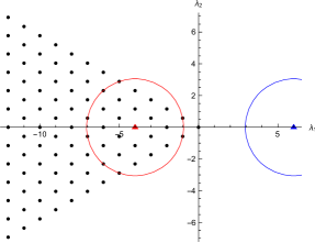
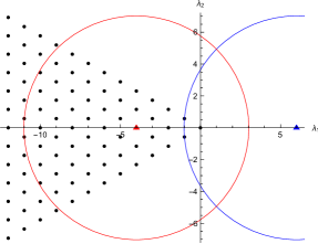
Figure 1: States (black dots) and “energy shells” (blue for $g{=}3$, red for $g{=}{-}2$) in weight space for $E={\textstyle\frac{28}{3}}$ (left) and $E={\textstyle\frac{148}{3}}$ (right).

Since $\mu_{2}=0$, we have an obvious energy degeneracy for

$$|n_{1},n_{2}\rangle_{g}{\quad{\rm and}\quad}|n_{1},n_{1}{-}n_{2}\rangle_{g}$$ (5.10)

except for $n_{1}{=}2n_{2}$, of course. For $g\geq 0$ there rarely appears higher degeneracy, but at $g<0$ energy levels are up to 12-fold degenerate! This plethora of states becomes physical only after the $\cal PT$ deformation and greatly enlarges the Hilbert space ${\cal H}_{g}$ for any $g{>}0$. Figure 2 displays the energy spectra with degeneracies for low levels and small integral values of $g$.

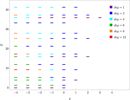
Figure 2: Low-lying energy spectrum and degeneracies (color-coded) for the $A_{2}$ model at integer coupling $g\in\mathbb{Z}$ in the range $g\in[-4,+4]$.

The basic intertwiner for the $A_{2}$ model is of order three,

$$M_{3}(g)\ =\ {\textstyle\frac{1}{3}}\,\textrm{res}\,\bigl{(}D_{12}D_{23}D_{31}+D_{23}D_{31}D_{12}+D_{31}D_{12}D_{23}\bigr{)}(g)$$ (5.11)

with the obvious notation $D_{ij}=D_{i}{-}D_{j}$. It computes to

$$M_{3}(g) \ =\ \partial_{12}\partial_{23}\partial_{31}-2g\,\bigl{\{}\cot q_{12}\partial_{23}\partial_{31}+\textrm{cyclic}\bigr{\}}+4g^{2}\bigl{(}\{\cot q_{12}\cot q_{23}\partial_{31}+\textrm{cyclic}\bigr{\}}$$ (5.12)

$$\quad-g(g{-}1)\bigl{\{}\sin^{-2}\!q_{31}\partial_{31}+\textrm{cyclic}\bigr{\}}-4g(2g{-}1)\bigl{\{}\sin q_{12}\sin q_{23}\sin q_{31}\bigr{\}}^{-1}$$

$$\quad-2g(3g^{2}{-}g{+}2)\cot q_{12}\cot q_{23}\cot q_{31}+2g(g{-}1)(g{+}2)\bigl{\{}\cot^{3}q_{12}+\textrm{cyclic}\bigr{\}}$$

where we abbreviated $\partial_{ij}={\textstyle\frac{\partial}{\partial q_{i}}}{-}{\textstyle\frac{\partial}{\partial q_{j}}}$ and $q_{ij}=q_{i}{-}q_{j}$. In terms of the multiplicative variables, the shift operator takes the form

$$M_{3}(g) \ \propto\ (x_{1}\partial_{1}{-}x_{2}\partial_{2})(x_{2}\partial_{2}{-}x_{3}\partial_{3})(x_{3}\partial_{3}{-}x_{1}\partial_{1})-g\bigl{\{}{\textstyle\frac{x_{1}+x_{2}}{x_{1}-x_{2}}}(x_{2}\partial_{2}{-}x_{3}\partial_{3})(x_{3}\partial_{3}{-}x_{1}\partial_{1})+\textrm{cyclic}\bigr{\}}$$ (5.13)

$$\quad+g^{2}\bigl{\{}{\textstyle\frac{x_{1}+x_{2}}{x_{1}-x_{2}}}{\textstyle\frac{x_{2}+x_{3}}{x_{2}-x_{3}}}(x_{3}\partial_{3}{-}x_{1}\partial_{1})+\textrm{cyclic}\bigr{\}}-g(g{-}1)\bigl{\{}{\textstyle\frac{x_{3}x_{1}}{x_{31}^{2}}}(x_{3}\partial_{3}{-}x_{1}\partial_{1})+\textrm{cyclic}\bigr{\}}$$

$$\quad+4g(2g{-}1){\textstyle\frac{x_{1}x_{2}x_{3}}{x_{12}x_{23}x_{31}}}-{\textstyle\frac{1}{4}}g(3g^{2}{-}g{+}2){\textstyle\frac{x_{1}+x_{2}}{x_{1}-x_{2}}}{\textstyle\frac{x_{2}+x_{3}}{x_{2}-x_{3}}}{\textstyle\frac{x_{3}+x_{1}}{x_{3}-x_{1}}}$$

$$\quad+{\textstyle\frac{1}{4}}g(g{-}1)(g{+}2)\bigl{\{}\bigl{(}{\textstyle\frac{x_{1}{+}x_{2}}{x_{1}{-}x_{2}}}\bigr{)}^{3}+\textrm{cyclic}\bigr{\}}\ .$$

It action on the states is

$$M_{3}(g)\,|n_{1},n_{2}\rangle_{g}\ \propto\ |n_{1}{-}2,n_{2}{-}1\rangle_{g+1}$$ (5.14)

conserving the energy. In weight space it moves $(\lambda_{1},\lambda_{2})\mapsto(\lambda_{1}{+}2,\lambda_{2})$.

For homogeneous intertwining relations, we redefine

$$C_{1}=I_{1}\ ,\quad C_{2}=I_{2}-2E_{0}=-2\,H{\quad{\rm and}\quad}C_{3}=I_{3}-I_{1}I_{2}$$ (5.15)

which obey

$$M_{3}(g)\,C_{k}(g)\ =\ C_{k}(g{+}1)\,M_{3}(g)\ .$$ (5.16)

This imples that the eigenvalue of $C_{3}$ is also conserved under the shift action. Indeed, it is readily verified that

$$C_{1}\,|n_{1},n_{2}\rangle_{g}\ =\ 0\ , C_{2}(g)\,|n_{1},n_{2}\rangle_{g}\ =\ -2\bigl{[}(n_{1}{+}2g)^{2}+{\textstyle\frac{1}{3}}(n_{1}{-}2n_{2})^{2}\bigr{]}\,|n_{1},n_{2}\rangle_{g}\ ,$$ (5.17)

$$C_{3}(g)\,|n_{1},n_{2}\rangle_{g} \ =\ -{\textstyle\frac{8}{9}}{\mathrm{i}}\,(n_{1}{-}2n_{2})(2n_{1}{-}n_{2}{+}3g)(n_{1}{+}n_{2}{+}3g)\,|n_{1},n_{2}\rangle_{g}\ ,$$

which is compatible with the shift (5.14). The degeneracy reflection $n_{2}\mapsto n_{1}{-}n_{2}$ flips the sign of $C_{3}$, so two such states can be discriminated by their $C_{3}$ eigenvalues.

As expected, the composition of the intertwiner with its adjoint yields an expression in the Liouville charges,

$$M_{3}^{\dagger}M_{3}(g) \ \propto\ 18I_{3}^{2}{-}36I_{3}I_{2}I_{1}{+}8I_{3}I_{1}^{3}{-}3I_{2}^{3}{+}21I_{2}^{2}I_{1}^{2}{-}9I_{2}I_{1}^{4}{+}I_{1}^{6}+2g^{2}(9I_{2}^{2}{-}6I_{2}I_{1}^{2}{+}I_{1}^{4})$$ (5.18)

$$\ =\ 18C_{3}^{2}+8C_{3}C_{1}^{3}-3C_{2}^{3}+3C_{2}^{2}C_{1}^{2}-C_{2}C_{1}^{4}+C_{1}^{6}$$

$$\qquad-6g^{2}(3C_{2}-C_{1}^{2}+8g^{2})^{2}\ .$$

Let us take a look at the extra degeneracy between even ($g{>}0$) and odd ($g{\leq}0$) states appearing when $g\in\mathbb{Z}$. The odd operator $Q_{3}(g)$ mapping one to the other and defined in (4.11) is of order $3(2g{-}1)$ and shifts the quantum numbers as

$$\bigl{(}n_{1},n_{2}\bigr{)}\ \mapsto\ \bigl{(}n_{1}{-}4g{+}2,n_{2}{-}2g{+}1\bigr{)}\ ,$$ (5.19)

which produces a rather large kernel. $Q_{3}$ commutes with all conserved charges $I_{k}$, so it keeps their eigenvalues. In weight space, it maps between the ‘even’ and ‘odd’ energy shells.

Finally, we briefly discuss two other kinds of $\cal PT$ deformations in the $A_{2}$-model context, which we denote as ‘angular’ and ‘radial’, respectively. Different from the parity transformation in (2.7), which amounts to the outer conjugation automorphism of $A_{N-1}$, the angular and radial deformations are compatible with an elementary Coxeter reflection (or particle permutation), e.g.

$${\cal P}:\quad(q_{1},q_{2},q_{3})\mapsto(q_{2},q_{1},q_{3}){\qquad{\rm and}\qquad}(x_{1},x_{2},x_{3})\mapsto(x_{2},x_{1},x_{3})\ ,$$ (5.20)

while $\cal T$ remains complex conjugation.

The angular $\cal PT$ deformation is homogeneous in the $q_{i}$ coordinates, in contrast to the constant complex coordinate shift (2.8). It is induced by a complex orthogonal coordinate change, $\vec{q}\mapsto\Gamma_{\epsilon}\vec{q}$ with $\Gamma_{\epsilon}\in\textrm{SO}(3,\mathbb{C})$ modulo SO$(3,\mathbb{R})$, described in [6]. Explicitly,

$$q_{i}\ \mapsto\ q_{i}^{\epsilon}\ =\ {\textstyle\frac{1}{3}}\bigl{[}(1{+}2\cosh\epsilon)\,q_{i}+(1{-}\cosh\epsilon-{\mathrm{i}}\sqrt{3}\sinh\epsilon)\,q_{j}+(1{-}\cosh\epsilon+{\mathrm{i}}\sqrt{3}\sinh\epsilon)\,q_{k}\bigr{]}$$ (5.21)

with $(i,j,k)$ being a cyclic permutation of $(1,2,3)$. This deformation does not entirely remove the singular loci of the potential given by

$$0\ =\ \sin q_{ij}^{\epsilon} \ =\ \cosh(\sqrt{3}\sinh\epsilon\,q_{k})\,\sin(\cosh\epsilon\,q_{ij})+{\mathrm{i}}\,\sinh(\sqrt{3}\sinh\epsilon\,q_{k})\,\cos(\cosh\epsilon\,q_{ij})$$ (5.22)

$$\ \Leftrightarrow\qquad q_{ij}=\frac{\ell\,\pi}{\cosh\epsilon}\quad\wedge\quad q_{k}=0\quad{\quad{\rm for}\quad}\ell=0,1,2,\ldots\ ,$$

where again $(i,j,k)$ are cyclic and we went to the conter-of-mass frame, so $q_{ik}+q_{jk}=-3q_{k}$. For small enough $\epsilon$, only the origin $\{q_{i}=0\}$ remains singular, but with growing value of $\epsilon$ extra singularities appear inside the Weyl alcove.

The radial $\cal PT$ deformation is a nonlinear one,

$$q_{i}\ \mapsto\ q_{i}^{\epsilon}\ =\ q_{i}+{\mathrm{i}}\epsilon\,q_{jk}/r\quad{\quad{\rm with}\quad}r^{2}=q_{12}^{2}+q_{23}^{2}+q_{31}^{2}$$ (5.23)

and $(i,j,k)$ being cyclic once more. The remaining singularities occur ar

$$q_{ij}=\ell\,\pi\quad\wedge\quad q_{k}=0\quad{\quad{\rm for}\quad}\ell=0,1,2,\ldots\ ,$$ (5.24)

and in addition one should average the potential, $V\mapsto V_{\epsilon}+V_{-\epsilon}$ with $V_{\epsilon}(q)=V(q^{\epsilon})$. Both cases can be parametrized jointly by writing

$$V_{\epsilon}(q_{ij})\ =\ V\bigl{(}R(\epsilon)\,q_{ij}+{\mathrm{i}}I(\epsilon)\,q_{k}\bigr{)}\quad{\quad{\rm with}\quad}\begin{cases}\phantom{-}R(\epsilon)=\cosh\epsilon\!\!\!\!\!\!&{\quad{\rm and}\quad}I(\epsilon)=\sqrt{3}\sinh\epsilon\\[4.0pt] \phantom{-}R(\epsilon)\ =\ 1&{\quad{\rm and}\quad}I(\epsilon)=-3/r\end{cases}$$ (5.25)

for the angular and radial $\cal PT$ deformation, respectively.

6 Details of the $G_{2}$ model

For a more complicated and non-simply-laced example, we turn to the $G_{2}$ model [11, 12] for three particles on a circle and apply the constant-shift $\cal PT$ deformation (2.8) but suppress it notationally. The $G_{2}$ model adds to the previous two-body potential of the $A_{2}$ case (5.1) a specific three-body interaction,

$$H(g) \ =\ -\frac{1}{2}\sum^{3}_{i=1}\frac{\partial}{\partial q_{i}^{2}}+\sum_{i<j}\frac{g_{\textrm{S}}(g_{\textrm{S}}{-}1)}{\sin^{2}(q_{i}{-}q_{j})}+\sum_{i<j}\frac{3g_{\textrm{L}}(g_{\textrm{L}}{-}1)}{\sin^{2}(q_{i}{+}q_{j}{-}2q_{k})}$$ (6.1)

$$\ =\ 2\sum^{3}_{i=1}(x_{i}\partial_{i})^{2}-4\,g_{\textrm{S}}(g_{\textrm{S}}{-}1)\sum_{i<j}\frac{x_{i}\,x_{j}}{(x_{i}{-}x_{j})^{2}}-12\,g_{\textrm{L}}(g_{\textrm{L}}{-}1)\sum_{i<j}\frac{x_{i}\,x_{j}\,x_{k}^{2}}{(x_{i}x_{j}{-}x_{k}^{2})^{2}}\ ,$$

where the index ‘$k$’ complements $i$ and $j$ to the triple (1,2,3), there are two independent real couplings $g_{\textrm{S}}$ and $g_{\textrm{L}}$, and we again put $L=\pi$ for simplicity. The potential can be viewed as a sum of two copies of the $A_{2}$ potential, with a relative coordinate rotation between them. The singular walls appear for

$$q_{i}-q_{j}=0{\qquad{\rm and}\qquad}q_{k}={\textstyle\frac{1}{3}}(q_{1}{+}q_{2}{+}q_{3})\quad{\quad{\rm for}\quad}i,j,k\in\{1,2,3\}\ ,$$ (6.2)

bounding the $G_{2}$ Weyl chambers. The Weyl group is enhanced from $S_{3}$ to $D_{6}$, generated by

$$s_{12}:\ (q_{1},q_{2},q_{3})\mapsto(q_{2},q_{1},q_{3}){\quad{\rm and}\quad}\jmath:\ (q_{1},q_{2},q_{3})\mapsto{\textstyle\frac{2}{3}}(q_{1}{+}q_{2}{+}q_{3})(1,1,1)-(q_{1},q_{2},q_{3})$$ (6.3)

and permutations, which for the $x_{i}$ coordinates translates to

$$s_{12}:\ (x_{1},x_{2},x_{3})\mapsto(x_{2},x_{1},x_{3}){\quad{\rm and}\quad}\jmath:\ (x_{1},x_{2},x_{3})\mapsto(x_{1}x_{2}x_{3})^{2/3}({\textstyle\frac{1}{x_{1}}},{\textstyle\frac{1}{x_{2}}},{\textstyle\frac{1}{x_{3}}})\ .$$ (6.4)

The Hamiltonian (6.1) yields eigenvalues

$$E_{n_{1},n_{2}}(g) \ =\ {\textstyle\frac{4}{3}}(n_{1}^{2}+n_{2}^{2}-n_{1}n_{2})+4g_{\textrm{S}}\,n_{1}+4g_{\textrm{L}}\,(2n_{1}-n_{2})+4({g_{\textrm{S}}^{2}}+3{g_{\textrm{L}}^{2}}+3g_{\textrm{S}}g_{\textrm{L}})$$ (6.5)

$$\ =\ (n_{1}+2g_{\textrm{S}}+3g_{\textrm{L}})^{2}+{\textstyle\frac{1}{3}}(n_{1}-2n_{2}+3g_{\textrm{L}})^{2}\quad{\quad{\rm with}\quad}n_{1}\geq 2n_{2}\geq 0\ ,$$

and the ground-state wave function for $g_{\textrm{S}}\geq 0$ and $g_{\textrm{L}}\geq 0$ is

$$\langle x|0,0\rangle_{g_{\textrm{S}},g_{\textrm{L}}}\ \equiv\ \Psi_{0}^{(g_{\textrm{S}},g_{\textrm{L}})}(x)\ =\ {\Delta\vphantom{\big{|}}}_{\textrm{S}}^{g_{\textrm{S}}}{\Delta\vphantom{\big{|}}}_{\textrm{L}}^{g_{\textrm{L}}}\quad{\quad{\rm with}\quad}E_{0}(g)=4\,({g_{\textrm{S}}^{2}}+3{g_{\textrm{L}}^{2}}+3g_{\textrm{S}}g_{\textrm{L}})\ ,$$ (6.6)

where we introduced

$${\Delta\vphantom{\big{|}}}_{\textrm{S}} \ =\ \frac{(x_{1}{-}x_{2})(x_{1}{-}x_{3})(x_{2}{-}x_{3})}{x_{1}\,x_{2}\,x_{3}}\ =\ Q^{-}_{2,1}\ ,$$ (6.7)

$${\Delta\vphantom{\big{|}}}_{\textrm{L}} \ =\ \frac{(x_{1}^{2}{-}x_{2}x_{3})(x_{2}^{2}{-}x_{1}x_{3})(x_{3}^{2}{-}x_{1}x_{2})}{x_{1}^{2}\,x_{2}^{2}\,x_{3}^{2}}\ =\ {\textstyle\frac{1}{2}}\bigl{(}Q^{+}_{3,0}-Q^{+}_{3,3}\bigr{)}\ .$$

In addition to the permutation symmetry inherited from the $A_{2}$ model, we also have to impose (anti-)invariance under the additional (even) Coxeter element $\jmath$ in (6.4), which implements an inversion in $x$ space and flips the sign of the roots by a $\pi$ rotation in the relative $q$ space. Noting that $\jmath^{2}=1$ and $[\jmath,s_{ij}]=0$ and

$$j:Q^{\pm}_{m_{1},m_{2}}\ \mapsto\ \pm Q^{\pm}_{m_{1},m_{1}{-}m_{2}}$$ (6.8)

one sees that $j$ flips the sign of both ${\Delta\vphantom{\big{|}}}_{S}$ and ${\Delta\vphantom{\big{|}}}_{L}$, hence

$$j\,\Psi_{0}^{(g_{\textrm{S}},g_{\textrm{L}})}(x)\ =\ (-)^{g_{\textrm{S}}+g_{\textrm{L}}}\Psi_{0}^{(g_{\textrm{S}},g_{\textrm{L}})}(x)\ .$$ (6.9)

We also deduce that the energy-degenerate states $|n_{1},n_{2}\rangle$ and $|n_{1},n_{1}{-}n_{2}\rangle$ of the $A_{2}$ model are related by the action of $j$. Therefore, only their sum or difference will be a $G_{2}$-model state, so the range of $n_{2}$ can be restricted to $n_{2}\leq{\textstyle\frac{1}{2}}n_{1}$, as already claimed in (6.5).

The excited states then take the form

$$\Psi_{n_{1},n_{2}}^{(g_{\textrm{S}},g_{\textrm{L}})}(x)\ =\ R_{n_{1},n_{2}}^{(g_{\textrm{S}},g_{\textrm{L}})}(x)\,\Psi_{0}^{(g_{\textrm{S}},g_{\textrm{L}})}(x)\ ,$$ (6.10)

where the $R_{n_{1},n_{2}}^{(g_{\textrm{S}},g_{\textrm{L}})}$ are again particular Weyl-symmetric rational functions of degree zero. Appendix D contains a list of low-lying wave functions.

Each eigenstate $|n_{1},n_{2}\rangle$ corresponds to a point

$$(\lambda_{1},\lambda_{2})=\bigl{(}-n_{1},{\textstyle\frac{1}{\sqrt{3}}}(n_{1}{-}2n_{2})\bigr{)}\quad{\quad{\rm with}\quad}\lambda_{1}\leq-\sqrt{3}\,\lambda_{2}\leq 0$$ (6.11)

in a ${\textstyle\frac{\pi}{6}}$ wedge above the negative $\lambda_{1}$ axis, in accord with one $G_{2}$ Weyl chamber. The circles determining the energy eigenstates for couplings $(g_{\textrm{S}},g_{\textrm{L}})$, $(1{-}g_{\textrm{S}},g_{\textrm{L}})$, $(g_{\textrm{S}},1{-}g_{\textrm{L}})$ and $(1{-}g_{\textrm{S}},1{-}g_{\textrm{L}})$ are centered at

$$(2g_{\textrm{S}}{+}3g_{\textrm{L}},-\sqrt{3}g_{\textrm{L}})\ ,\quad(2{-}2g_{\textrm{S}}{+}3g_{\textrm{L}},-\sqrt{3}g_{\textrm{L}})\ ,$$ (6.12)

$$(3{+}2g_{\textrm{S}}{-}3g_{\textrm{L}},\sqrt{3}g_{\textrm{L}}{-}\sqrt{3})\ ,\quad(5{-}2g_{\textrm{S}}{-}3g_{\textrm{L}},\sqrt{3}g_{\textrm{L}}{-}\sqrt{3})$$

in $\lambda$-space, respectively. This is illustrated in Figure 3.

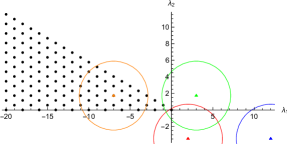
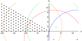
Figure 3: States (black dots) and “energy shells” for $(g_{\textrm{S}},g_{\textrm{L}})\,{=}(3,2)$ (blue), ${=}({-}2,2)$ (red), ${=}(3,{-}1)$ (green) and ${=}({-}2,{-}1)$ (orange) for $E={\textstyle\frac{52}{3}}$ (left) and $E=156$ (right).

After the $\cal PT$ deformation, the Hilbert space ${\cal H}_{g_{\textrm{S}},g_{\textrm{L}}}$ comprises the four towers obtained from the four circles in Figure 3. Again, for integral values of the couplings, the towers have matching energy levels, which greatly increases their degeneracy.

The $G_{2}$ Dunkl operator is an extension of the $A_{2}$ one (again with $\{i,j,k\}=\{1,2,3\}$),

$$-{\mathrm{i}}\,D_{i}(g)\ =\ 2\,x_{i}\partial_{i}-g_{\textrm{S}}\sum_{j(\neq i)}\frac{x_{i}{+}x_{j}}{x_{i}{-}x_{j}}\,s_{ij}-g_{\textrm{L}}\biggl{(}\sum_{j(\neq i)}\frac{x_{i}x_{j}{+}x_{k}^{2}}{x_{i}x_{j}{-}x_{k}^{2}}\,s_{ik}-2\,\frac{x_{j}x_{k}{+}x_{i}^{2}}{x_{j}x_{k}{-}x_{i}^{2}}\,s_{jk}\biggr{)}\jmath\ .$$ (6.13)

The first two Newton sums in this Dunkl operator yield the conserved momentum and energy,

$$I_{1}\ =\ \textrm{res}\sum_{i}D_{i}\ =\ {\mathrm{i}}\,P{\qquad{\rm and}\qquad}I_{2}\ =\ \textrm{res}\sum_{i}D_{i}^{2}\ =\ -2(H-E_{0})\ ,$$ (6.14)

because $\sum_{i}q_{i}$ and $\sum_{i}q_{i}^{2}$ are not only permutation-symmetric but also invariant under the rotation $\jmath$ from (6.3). This, however, is not the case for $\sum_{i}q_{i}^{r}$ when $r{\geq}3$, but one can find a Weyl-invariant combination at order six,

$$\sigma_{3}\,\jmath\,\sigma_{3}\ =\ \sigma_{3}(\sigma_{3}-2\sigma_{2}\sigma_{1}+{\textstyle\frac{4}{9}}\sigma_{1}^{3})\quad{\quad{\rm with}\quad}\sigma_{r}=\textstyle{\sum_{i}}q_{i}^{r}\ ,$$ (6.15)

which generates another Liouville charge,

$$J_{6}\ =\ \textrm{res}\bigl{\{}5D_{1}^{6}+12D_{1}^{5}D_{2}+12D_{1}^{4}D_{2}^{2}-24D_{1}^{4}D_{2}D_{3}+10D_{1}^{3}D_{2}^{3}+12D_{1}^{3}D_{2}^{2}D_{3}$$ (6.16)

$$\qquad\qquad+\ \textrm{permutations(1,2,3)}\bigr{\}}_{\textrm{symmetrized}}$$

$$\ =\ 5(x_{1}\partial_{1})^{6}+12(x_{1}\partial_{1})^{5}x_{2}\partial_{2}+12(x_{1}\partial_{1})^{4}(x_{2}\partial_{2})^{2}$$

$$\quad-24(x_{1}\partial_{1})^{4}(x_{2}\partial_{2})(x_{3}\partial_{3})+10(x_{1}\partial_{1})^{3}(x_{2}\partial_{2})^{3}+12(x_{1}\partial_{1})^{3}(x_{2}\partial_{2})^{2}(x_{3}\partial_{3})$$

$$\quad+c_{400}{\cdot}(x_{1}\partial_{1})^{4}+c_{310}{\cdot}(x_{1}\partial_{1})^{3}x_{2}\partial_{2}+c_{220}{\cdot}(x_{1}\partial_{1})^{2}(x_{2}\partial_{2})^{2}+c_{211}{\cdot}(x_{1}\partial_{1})^{2}(x_{2}\partial_{2})(x_{3}\partial_{3})$$

$$\quad+c_{300}{\cdot}(x_{1}\partial_{1})^{3}+c_{210}{\cdot}(x_{1}\partial_{1})^{2}(x_{2}\partial_{2})+c_{111}{\cdot}(x_{1}\partial_{1})(x_{2}\partial_{2})(x_{3}\partial_{3})$$

$$\quad+c_{200}{\cdot}(x_{1}\partial_{1})^{2}+c_{110}{\cdot}(x_{1}\partial_{1})(x_{2}\partial_{2})+c_{100}{\cdot}(x_{1}\partial_{1})+c_{000}+\ \textrm{permutations(1,2,3)}$$

where symmetrization means Weyl ordering of every summand, and the coefficients $c_{s_{1}s_{2}s_{3}}(x)$ are given in Appendix E.

From (6.8) we see that the $G_{2}$ model enjoys two separate intertwiners,

$$M_{3,\textrm{S}} \ =\ {\textstyle\frac{1}{3}}\,\textrm{res}\,(D_{1}{-}D_{2})(D_{2}{-}D_{3})(D_{3}{-}D_{1})\ +\textrm{cyclic}\ ,$$ (6.17)

$$M_{3,\textrm{L}} \ =\ {\textstyle\frac{1}{3}}\,\textrm{res}\,(D_{1}{+}D_{2}{-}2D_{3})(D_{2}{+}D_{3}{-}2D_{1})(D_{3}{+}D_{1}{-}2D_{2})\ +\textrm{cyclic}\ ,$$

which independently shift by unity the couplings $g_{\textrm{S}}$ and $g_{\textrm{L}}$, respectively,

$$M_{3,\textrm{S}}\,|n_{1},n_{2}\rangle_{g_{\textrm{S}},g_{\textrm{L}}} \propto\ |n_{1}{-}2,n_{2}{-}1\rangle_{g_{\textrm{S}}+1,g_{\textrm{L}}}\ ,$$ (6.18)

$$M_{3,\textrm{L}}\,|n_{1},n_{2}\rangle_{g_{\textrm{S}},g_{\textrm{L}}} \propto\ |n_{1}{-}3,n_{2}\rangle_{g_{\textrm{S}},g_{\textrm{L}}+1}\ .$$

Their explicit form is

$$M_{3,\textrm{S}} \ \propto\ (x_{1}\partial_{1}{-}x_{2}\partial_{2})(x_{2}\partial_{2}{-}x_{3}\partial_{3})(x_{3}\partial_{3}{-}x_{1}\partial_{1})-g_{\textrm{S}}\bigl{\{}{\textstyle\frac{x_{1}+x_{2}}{x_{1}-x_{2}}}(x_{2}\partial_{2}{-}x_{3}\partial_{3})(x_{3}\partial_{3}{-}x_{1}\partial_{1})+\textrm{cyclic}\bigr{\}}$$ (6.19)

$$\quad+{g_{\textrm{S}}^{2}}\bigl{\{}{\textstyle\frac{x_{1}+x_{2}}{x_{1}-x_{2}}}{\textstyle\frac{x_{2}{+}x_{3}}{x_{2}{-}x_{3}}}(x_{3}\partial_{3}{-}x_{1}\partial_{1})+\textrm{cyclic}\bigr{\}}-g_{\textrm{S}}(g_{\textrm{S}}{-}1)\bigl{\{}{\textstyle\frac{x_{3}x_{1}}{x_{31}^{2}}}(x_{3}\partial_{3}{-}x_{1}\partial_{1})+\textrm{cyclic}\bigr{\}}$$

$$\quad+9g_{\textrm{L}}(g_{\textrm{L}}{-}1)\bigl{\{}{\textstyle\frac{x_{2}^{2}x_{3}x_{1}}{(x_{2}^{2}{-}x_{3}x_{1})^{2}}}(x_{3}\partial_{3}{-}x_{1}\partial_{1})+\textrm{cyclic}\bigr{\}}+2g_{\textrm{S}}(4g_{\textrm{S}}{-}2{+}9g_{\textrm{L}}(g_{\textrm{L}}{+}1)){\textstyle\frac{x_{1}x_{2}x_{3}}{x_{12}x_{23}x_{31}}}$$

$$\quad-{\textstyle\frac{1}{4}}g_{\textrm{S}}(3{g_{\textrm{S}}^{2}}{-}g_{\textrm{S}}{+}2){\textstyle\frac{x_{1}{+}x_{2}}{x_{1}{-}x_{2}}}{\textstyle\frac{x_{2}+x_{3}}{x_{2}-x_{3}}}{\textstyle\frac{x_{3}{+}x_{1}}{x_{3}{-}x_{1}}}+{\textstyle\frac{1}{4}}g_{\textrm{S}}(g_{\textrm{S}}{-}1)(g_{\textrm{S}}{+}2)\bigl{\{}\bigl{(}{\textstyle\frac{x_{1}{+}x_{2}}{x_{1}{-}x_{2}}}\bigr{)}^{3}+\textrm{cyclic}\bigr{\}}$$

$$\quad-9g_{\textrm{S}}g_{\textrm{L}}(g_{\textrm{L}}{+}1)\bigl{\{}{\textstyle\frac{x_{3}{+}x_{1}}{x_{3}-x_{1}}}{\textstyle\frac{x_{2}^{2}x_{3}x_{1}}{(x_{2}^{2}{-}x_{3}x_{1})^{2}}}+\textrm{cyclic}\bigr{\}}\ ,$$

$$M_{3,\textrm{L}} \ \propto\ (x_{1}\partial_{1}{+}x_{2}\partial_{2}{-}2x_{3}\partial_{3})(x_{2}\partial_{2}{+}x_{3}\partial_{3}{-}2x_{1}\partial_{1})(x_{3}\partial_{3}{+}x_{1}\partial_{1}{-}2x_{2}\partial_{2})$$ (6.20)

$$\quad+3g_{\textrm{L}}\bigl{\{}{\textstyle\frac{x_{2}^{2}{+}x_{3}x_{1}}{x_{2}^{2}{-}x_{3}x_{1}}}(x_{1}\partial_{1}{+}x_{2}\partial_{2}{-}2x_{3}\partial_{3})(x_{2}\partial_{2}{+}x_{3}\partial_{3}{-}2x_{1}\partial_{1})+\textrm{cyclic}\bigr{\}}$$

$$\quad+9g_{\textrm{L}}\bigl{\{}x_{1}x_{2}\bigl{[}{\textstyle\frac{(g_{\textrm{L}}-1)x_{2}x_{3}}{(x_{2}^{2}{-}x_{1}x_{3})^{2}}}+{\textstyle\frac{(g_{\textrm{L}}-1)x_{1}x_{3}}{(x_{1}^{2}{-}x_{2}x_{3})^{2}}}+{\textstyle\frac{2g_{\textrm{L}}(x_{3}^{2}{+}x_{1}x_{2})}{(x_{2}^{2}{-}x_{1}x_{3})(x_{1}^{2}{-}x_{2}x_{3})}}\bigr{]}(x_{1}\partial_{1}{+}x_{2}\partial_{2}{-}2x_{3}\partial_{3})+\textrm{cyclic}\bigr{\}}$$

$$\quad+9g_{\textrm{S}}(g_{\textrm{S}}{-}1)\bigl{\{}{\textstyle\frac{x_{1}x_{2}}{(x_{1}{-}x_{2})^{2}}}(x_{1}\partial_{1}{+}x_{2}\partial_{2}{-}2x_{3}\partial_{3})+\textrm{cyclic}\bigr{\}}-27g_{\textrm{L}}g_{\textrm{S}}(g_{\textrm{S}}{-}1)\bigl{\{}{\textstyle\frac{x_{1}x_{2}}{(x_{1}{-}x_{2})^{2}}}+\textrm{cyclic}\bigr{\}}$$

$$\quad+54g_{\textrm{L}}\bigl{[}g_{\textrm{S}}(g_{\textrm{S}}{-}1){\textstyle\frac{(x_{1}^{2}{-}x_{2}x_{3}{+}x_{2}^{2}{-}x_{3}x_{1}{+}x_{3}^{2}{-}x_{1}x_{2})^{3}}{(x_{1}-x_{2})^{2}(x_{2}-x_{3})^{2}(x_{3}-x_{1})^{2}}}-g_{\textrm{L}}(g_{\textrm{L}}{-}3)\bigr{]}{\textstyle\frac{x_{1}^{2}x_{2}^{2}x_{3}^{2}}{(x_{1}^{2}{-}x_{2}x_{3})(x_{2}^{2}{-}x_{3}x_{1})(x_{3}^{2}{-}x_{1}x_{2})}}$$

$$\quad-27g_{\textrm{L}}({g_{\textrm{L}}^{2}}{+}g_{\textrm{L}}{-}2)x_{1}x_{2}x_{3}\bigl{\{}x_{1}{\textstyle\frac{x_{1}^{2}+x_{2}x_{3}}{x_{1}^{2}{-}x_{2}x_{3}}}+\textrm{cyclic}\bigr{\}}+27{g_{\textrm{L}}^{3}}{\textstyle\frac{(x_{1}^{2}{+}x_{2}x_{3})(x_{2}^{2}{+}x_{3}x_{1})(x_{3}^{2}{+}x_{1}x_{2})}{(x_{1}^{2}{-}x_{2}x_{3})(x_{2}^{2}{-}x_{3}x_{1})(x_{3}^{2}{-}x_{1}x_{2})}}\ .$$

A better basis for the Liouville charges is

$$C_{1}=I_{1}\ ,\quad C_{2}=I_{2}-2E_{0}=-2\,H{\qquad{\rm and}\qquad}$$ (6.21)

$$C_{6} \ =\ J_{6}+2(27{g_{\textrm{L}}^{2}}+24g_{\textrm{L}}g_{\textrm{S}}+8{g_{\textrm{S}}^{2}})C_{2}C_{1}^{2}-9{g_{\textrm{L}}^{2}}C_{2}^{2}-{\textstyle\frac{1}{9}}(105{g_{\textrm{L}}^{2}}+96g_{\textrm{L}}g_{\textrm{S}}+32{g_{\textrm{S}}^{2}})C_{1}^{4}$$ (6.22)

$$\qquad+16(39{g_{\textrm{L}}^{4}}+72{g_{\textrm{L}}^{3}}g_{\textrm{S}}+60{g_{\textrm{L}}^{2}}{g_{\textrm{S}}^{2}}+24g_{\textrm{L}}g_{\textrm{S}}^{3}+4{g_{\textrm{S}}^{4}})C_{1}^{2}-144{g_{\textrm{L}}^{4}}C_{2}-576g_{\textrm{L}}^{6}\ ,$$

obeying homogeneous intertwining relations

$$M_{3,\textrm{S}}(g_{\textrm{S}},g_{\textrm{L}})\,C_{k}(g_{\textrm{S}},g_{\textrm{L}}) \ =\ C_{k}(g_{\textrm{S}}{+}1,g_{\textrm{L}})\,M_{3,\textrm{S}}\ ,$$ (6.23)

$$M_{3,\textrm{L}}(g_{\textrm{S}},g_{\textrm{L}})\,C_{k}(g_{\textrm{S}},g_{\textrm{L}}) \ =\ C_{k}(g_{\textrm{S}},g_{\textrm{L}}{+}1)\,M_{3,\textrm{L}}\ .$$

This is also signified by the action

$$C_{6}\,|n_{1},\!n_{2}\rangle_{g_{\textrm{S}},g_{\textrm{L}}}\ =\ -{\textstyle\frac{64}{81}}(3g_{\textrm{L}}{+}n_{1}{-}2n_{2})^{2}(6g_{\textrm{L}}{+}3g_{\textrm{S}}{+}2n_{1}{-}n_{2})^{2}(3g_{\textrm{L}}{+}3g_{\textrm{S}}+n_{1}{+}n_{2})^{2}|n_{1},\!n_{2}\rangle_{g_{\textrm{S}},g_{\textrm{L}}}.$$ (6.24)

The intertwining with their corresponding conjugates produces two polynomials in the Liouville charges,

$$M_{3,\textrm{S}}^{\dagger}M_{3,\textrm{S}} \ =\ -3C_{6}-{\textstyle\frac{1}{6}}C_{1}^{6}+{\textstyle\frac{3}{2}}C_{2}C_{1}^{4}-{\textstyle\frac{7}{2}}C_{2}^{2}C_{1}^{2}+{\textstyle\frac{1}{2}}C_{2}^{3}+{g_{\textrm{S}}^{2}}(C_{1}^{2}-3C_{2}-8{g_{\textrm{S}}^{2}})^{2}\ ,$$ (6.25)

$$M_{3,\textrm{L}}^{\dagger}M_{3,\textrm{L}} \ =\ 81C_{6}+C_{1}^{2}(2C_{1}^{2}-9C_{2})^{2}+81{g_{\textrm{L}}^{2}}(C_{1}^{2}-3C_{2}-24{g_{\textrm{L}}^{2}})^{2}\ .$$

The intertwining operators also enable odd conserved charges when the couplings take integer values, in the form of the chain of operators

$$Q_{3,\textrm{S}}(g_{\textrm{S}},g_{\textrm{L}}) \ =\ M_{3,\textrm{S}}(g_{\textrm{S}}{-}1,g_{\textrm{L}})M_{3,S}(g_{\textrm{S}}{-}2,g_{\textrm{L}})\cdots M_{3,S}(2{-}g_{\textrm{S}},g_{\textrm{L}})M_{3,S}(1{-}g_{\textrm{S}},g_{\textrm{L}})\ ,$$ (6.26)

$$Q_{3,\textrm{L}}(g_{\textrm{S}},g_{\textrm{L}}) \ =\ M_{3,\textrm{L}}(g_{\textrm{S}},g_{\textrm{L}}{-}1)M_{3,L}(g_{\textrm{S}},g_{\textrm{L}}{-}2)\cdots M_{3,L}(g_{\textrm{S}},2{-}g_{\textrm{L}})M_{3,L}(g_{\textrm{S}},1{-}g_{\textrm{L}})\ ,$$

which in the simplest non-trivial cases squares to the form of the polynomials in (6.25),

$$Q_{3,\textrm{S}}^{2}(2,g_{\textrm{L}}) \ =\ \left(3C_{6}+{\textstyle\frac{1}{6}}C_{1}^{6}-{\textstyle\frac{3}{2}}C_{2}C_{1}^{4}+{\textstyle\frac{7}{2}}C_{2}^{2}C_{1}^{2}-{\textstyle\frac{1}{2}}C_{2}^{3}\right)^{3}+\textrm{lower terms}\ ,$$ (6.27)

$$Q_{3,\textrm{L}}^{2}(g_{\textrm{S}},2) \ =\ \left(81C_{6}+4C_{1}^{2}(C_{1}^{2}-{\textstyle\frac{9}{2}}C_{2})^{2}\right)^{3}+\textrm{lower terms}\ .$$

Acknowledgments

This work was partially supported by the Alexander von Humboldt Foundation, Fondecyt grant 1171475 and by the Deutsche Forschungsgemeinschaft under grant LE 838/12. This article is based upon work from COST Action MP1405 QSPACE, supported by COST (European Cooperation in Science and Technology). O.L. is grateful for the warm hospitality at CECs and Universidad Austral de Chile, where the main part of this work was done. F.C. is also grateful for the warm hospitality at Leibniz Universität Hannover.

Appendix A Potential-free frame

We display some relations with the potential-free frame for the $A_{N-1}$ model. By conjugating the Hamiltonian one can trade the potential for a first-order derivative term,

$$\widetilde{H}(g)\ =\ {\Delta\vphantom{\big{|}}}^{-g}H(g)\,{\Delta\vphantom{\big{|}}}^{g} \ =\ -\frac{1}{2}\sum^{N}_{i=1}\frac{\partial}{\partial q_{i}^{2}}-\frac{\pi}{L}\,g\sum_{i<j}\cot{\textstyle\frac{\pi}{L}}(q_{i}{-}q_{j})\Bigl{(}\frac{\partial}{\partial q_{i}}-\frac{\partial}{\partial q_{j}}\Bigr{)}$$ (A.1)

$$\ =\ \frac{\pi^{2}}{L^{2}}\biggl{[}2\sum^{N}_{i=1}\Bigl{(}\frac{x_{i}\partial}{\partial x_{i}}\Bigr{)}^{2}+2\,g\sum_{i<j}\frac{x_{i}{+}x_{j}}{x_{i}{-}x_{j}}\bigl{(}x_{i}\partial_{i}-x_{j}\partial_{j}\bigr{)}\biggr{]}\ .$$

Appendix B Ring of Laurent polynomials

For convenience we describe the multiplication rule for the Laurent polynomials

$$Q^{\pm}_{m_{1},m_{2}}(y) \ =\ y_{1}^{2m_{1}-m_{2}}y_{2}^{2m_{2}-m_{1}}y_{3}^{-m_{1}-m_{2}}\pm y_{1}^{2m_{2}-m_{1}}y_{2}^{2m_{1}-m_{2}}y_{3}^{-m_{1}-m_{2}}+\ \textrm{cyclic}$$ (B.1)

$$\ =\ y_{1}^{\alpha}y_{2}^{\beta}y_{3}^{\gamma}+y_{1}^{\beta}y_{2}^{\gamma}y_{3}^{\alpha}+y_{1}^{\gamma}y_{2}^{\alpha}y_{3}^{\beta}\pm y_{1}^{\alpha}y_{2}^{\gamma}y_{3}^{\beta}\pm y_{1}^{\beta}y_{2}^{\alpha}y_{3}^{\gamma}\pm y_{1}^{\gamma}y_{2}^{\beta}y_{3}^{\alpha}$$

$$\ =:\ [m_{1},m_{2}]_{\pm}\ =:\ (\alpha,\beta,\gamma)_{\pm}\qquad{\quad{\rm with}\quad}\alpha+\beta+\gamma=0\ .$$

The relation between the parameters is

$$3m_{1}=2\alpha{+}\beta=-\beta{-}2\gamma=\alpha{-}\gamma{\qquad{\rm and}\qquad}3m_{2}=2\beta{+}\alpha=-\alpha{-}2\gamma=\beta{-}\gamma\ .$$ (B.2)

To remove the redundancy of the labelling, we stipulate that

$$m_{1}\geq m_{2}\geq 0\qquad\Leftrightarrow\qquad\alpha\geq\beta\geq\gamma\ .$$ (B.3)

It is immediate that $[m_{1},0]_{-}=[m_{1},m_{1}]_{-}=0$.

The obvious multiplication ($\epsilon,{\bar{\epsilon}}\in\{+,-\}$)

$$(\alpha,\beta,\gamma)_{\epsilon}\times(\bar{\alpha},\bar{\beta},\bar{\gamma})_{\bar{\epsilon}}\ =\$$ (B.4)

$$\qquad\quad(\alpha{+}\bar{\alpha},\beta{+}\bar{\beta},\gamma{+}\bar{\gamma})_{\epsilon\bar{\epsilon}}+(\alpha{+}\bar{\beta},\beta{+}\bar{\gamma},\gamma{+}\bar{\alpha})_{\epsilon\bar{\epsilon}}+(\alpha{+}\bar{\gamma},\beta{+}\bar{\alpha},\gamma{+}\bar{\beta})_{\epsilon\bar{\epsilon}}$$

$$\qquad+{\bar{\epsilon}}\,(\alpha{+}\bar{\alpha},\beta{+}\bar{\gamma},\gamma{+}\bar{\beta})_{\epsilon\bar{\epsilon}}+{\bar{\epsilon}}\,(\alpha{+}\bar{\beta},\beta{+}\bar{\alpha},\gamma{+}\bar{\gamma})_{\epsilon\bar{\epsilon}}+{\bar{\epsilon}}\,(\alpha{+}\bar{\gamma},\beta{+}\bar{\beta},\gamma{+}\bar{\alpha})_{\epsilon\bar{\epsilon}}$$

produces the law

$$[m_{1},m_{2}]_{\epsilon}\times[n_{1},n_{2}]_{\bar{\epsilon}}\ =\$$ (B.5)

$$\qquad\quad[m_{1}{+}n_{1},m_{2}{+}n_{2}]_{\epsilon\bar{\epsilon}}+[m_{1}{-}n_{1}{+}n_{2},m_{2}{-}n_{1}]_{\epsilon\bar{\epsilon}}+[m_{1}{-}n_{2},m_{2}{+}n_{1}{-}n_{2}]_{\epsilon\bar{\epsilon}}$$

$$\qquad+{\bar{\epsilon}}\,[m_{1}{+}n_{1}{-}n_{2},m_{2}{-}n_{2}]_{\epsilon\bar{\epsilon}}+{\bar{\epsilon}}\,[m_{1}{+}n_{2},m_{2}{+}n_{1}]_{\epsilon\bar{\epsilon}}+{\bar{\epsilon}}\,[m_{1}{-}n_{1},m_{2}{-}n_{1}{+}n_{2}]_{\epsilon\bar{\epsilon}}\ .$$

Even assuming $m_{1}\geq n_{1}$ (without loss of generality), the right-hand side may produce contributions $[k_{1},k_{2}]_{\pm}$ with $k_{1}<k_{2}$ or with $k_{2}<0$, which we outlawed. However, it is easy to see that

$$[k_{1},k_{2}]_{\pm}=\pm[k_{2},k_{1}]_{\pm}{\qquad{\rm and}\qquad}[k_{1},k_{2}]_{\pm}=\pm[k_{1}{-}k_{2},-k_{2}]_{\pm}\ ,$$ (B.6)

so one may employ the first relation in the first case and the second one in the second case to obtain an admissible result. Some examples are

$${}_{\pm}\times[0,0]_{+} \ =\ 6\,[m_{1},m_{2}]_{\pm}\ ,$$ (B.7)

$$[m_{1},m_{2}]_{\pm}\times[1,0]_{+} \ =\ 2\,[m_{1}{+}1,m_{2}]_{\pm}+2\,[m_{1},m_{2}{+}1]_{\pm}+2\,[m_{1}{-}1,m_{2}{-}1]_{\pm}\ ,$$

$$[m_{1},m_{2}]_{\pm}\times[1,1]_{+} \ =\ 2\,[m_{1}{+}1,m_{2}{+}1]_{\pm}+2\,[m_{1},m_{2}{-}1]_{\pm}+2\,[m_{1}{-}1,m_{2}]_{\pm}\ ,$$

$$[m_{1},m_{2}]_{\pm}\times[2,0]_{+} \ =\ 2\,[m_{1}{+}2,m_{2}]_{\pm}+2\,[m_{1},m_{2}{+}2]_{\pm}+2\,[m_{1}{-}2,m_{2}{-}2]_{\pm}\ ,$$

$$[m_{1},m_{2}]_{\pm}\times[2,2]_{+} \ =\ 2\,[m_{1}{+}2,m_{2}{+}2]_{\pm}+2\,[m_{1},m_{2}{-}2]_{\pm}+2\,[m_{1}{-}2,m_{2}]_{\pm}\ ,$$

$$[m_{1},m_{2}]_{\pm}\times[2,1]_{+} \ =\ [m_{1}{+}2,m_{2}{+}1]_{\pm}+[m_{1}{+}1,m_{2}{+}2]_{\pm}+[m_{1}{+}1,m_{2}{-}1]_{\pm}$$

$$\ \ +[m_{1}{-}1,m_{2}{+}1]_{\pm}+[m_{1}{-}1,m_{2}{-}2]_{\pm}+[m_{1}{-}2,m_{2}{-}1]_{\pm}\ ,$$

$$[m_{1},m_{2}]_{\pm}\times[2,1]_{-} \ =\ [m_{1}{+}2,m_{2}{+}1]_{\mp}-[m_{1}{+}1,m_{2}{+}2]_{\mp}-[m_{1}{+}1,m_{2}{-}1]_{\mp}$$

$$\ \ +[m_{1}{-}1,m_{2}{+}1]_{\mp}1+[m_{1}{-}1,m_{2}{-}2]_{\mp}-[m_{1}{-}2,m_{2}{-}1]_{\mp}\ .$$

Appendix C Wave functions for the $A_{2}$ model

The $A_{2}$ wave functions take the form

$$\langle x|n_{1},n_{2}\rangle_{g}\ \equiv\ \Psi_{n_{1},n_{2}}^{(g)}(x)\ =\ R_{n_{1},n_{2}}^{(g)}(x)\,{\Delta\vphantom{\big{|}}}^{g}\ =\ P_{n_{1},n_{2}}^{(g)}(x)\,(x_{1}x_{2}x_{3})^{-(n_{1}+n_{2})/3}\,{\Delta\vphantom{\big{|}}}^{g}\ ,$$ (C.1)

where $x=(x_{1},x_{2},x_{3})$ and $P_{n_{1},n_{2}}^{(g)}$ is a homogeneous permutation-symmetric Jack polynomial of degree $n_{1}{+}n_{2}$ in $x$. Passing to the more convenient variables

$$y_{i}=x_{i}^{1/3}$$ (C.2)

the rational function $R_{n_{1},n_{2}}^{(g)}$ is a linear combination of symmetric basis functions

$$Q^{+}_{m_{1},m_{2}}(y)\ =\ y_{1}^{2m_{1}-m_{2}}y_{2}^{2m_{2}-m_{1}}y_{3}^{-m_{1}-m_{2}}+y_{1}^{2m_{2}-m_{1}}y_{2}^{2m_{1}-m_{2}}y_{3}^{-m_{1}-m_{2}}+\ \textrm{cyclic}$$ (C.3)

$$\textrm{with}\quad m_{1}{+}m_{2}=n_{1}{+}n_{2}{-}3\ell{\quad{\rm for}\quad}\ell=0,1,2,\ldots\ .$$

The first few Laurent polynomials are

$$R_{0,0} =Q^{+}_{0,0}=6\ ,$$ (C.4)

$$R_{1,0} =Q^{+}_{1,0}=2\,(y_{1}^{2}y_{2}^{-1}y_{3}^{-1}{+}y_{2}^{2}y_{3}^{-1}y_{1}^{-1}{+}y_{3}^{2}y_{1}^{-1}y_{2}^{-1})\ ,$$

$$R_{1,1} =Q^{+}_{1,1}=2\,(y_{1}\,y_{2}\,y_{3}^{-2}{+}y_{2}\,y_{3}\,y_{1}^{-2}{+}y_{3}\,y_{1}\,y_{2}^{-2})\ ,$$

$$R_{2,0} =Q^{+}_{2,0}+{\textstyle\frac{2g}{g+1}}Q^{+}_{1,1}\ ,$$

$$R_{2,1} =Q^{+}_{2,1}+{\textstyle\frac{g}{2g+1}}Q^{+}_{0,0}\ ,$$

$$R_{2,2} =Q^{+}_{2,2}+{\textstyle\frac{2g}{g+1}}Q^{+}_{1,0}\ ,$$

$$R_{3,0} =Q^{+}_{3,0}+{\textstyle\frac{6g}{g+2}}Q^{+}_{2,1}+{\textstyle\frac{2g^{2}}{(g+1)(g+2)}}Q^{+}_{0,0}\ ,$$

$$R_{3,1} =Q^{+}_{3,1}+{\textstyle\frac{g}{g+1}}Q^{+}_{2,2}+{\textstyle\frac{g(5g+3)}{2(g+1)^{2}}}Q^{+}_{1,0}\ ,$$

$$R_{3,2} =Q^{+}_{3,2}+{\textstyle\frac{g}{g+1}}Q^{+}_{2,0}+{\textstyle\frac{g(5g+3)}{2(g+1)^{2}}}Q^{+}_{1,1}\ ,$$

$$R_{3,3} =Q^{+}_{3,3}+{\textstyle\frac{6g}{g+2}}Q^{+}_{2,1}+{\textstyle\frac{2g^{2}}{(g+1)(g+2)}}Q^{+}_{0,0}\ ,$$

$$R_{4,0} =Q^{+}_{4,0}+{\textstyle\frac{8g}{g+3}}Q^{+}_{3,1}+{\textstyle\frac{6g(g+1)}{(g+2)(g+3)}}Q^{+}_{2,2}+{\textstyle\frac{12g^{2}}{(g+2)(g+3)}}Q^{+}_{1,0}\ ,$$

$$R_{4,1} =Q^{+}_{4,1}+{\textstyle\frac{3g}{g+2}}Q^{+}_{3,2}+{\textstyle\frac{g(7g+8)}{(g+2)(2g+3)}}Q^{+}_{2,0}+{\textstyle\frac{3g(4g+1)}{(g+2)(2g+3)}}Q^{+}_{1,1}\ ,$$

$$R_{4,2} =Q^{+}_{4,2}+{\textstyle\frac{g}{g+1}}Q^{+}_{3,3}+{\textstyle\frac{g}{g+1}}Q^{+}_{3,0}+{\textstyle\frac{4g(4g+1)}{(g+1)(2g+3)}}Q^{+}_{2,1}+{\textstyle\frac{g(10g^{2}+7g+3)}{2(g+1)^{2}(2g+3)}}Q^{+}_{0,0}\ ,$$

$$R_{4,3} =Q^{+}_{4,3}+{\textstyle\frac{3g}{g+2}}Q^{+}_{3,1}+{\textstyle\frac{g(7g+8)}{(g+2)(2g+3)}}Q^{+}_{2,2}+{\textstyle\frac{3g(4g+1)}{(g+2)(2g+3)}}Q^{+}_{1,0}\ ,$$

$$R_{4,4} =Q^{+}_{4,4}+{\textstyle\frac{8g}{g+3}}Q^{+}_{3,2}+{\textstyle\frac{6g(g+1)}{(g+2)(g+3)}}Q^{+}_{2,0}+{\textstyle\frac{12g^{2}}{(g+2)(g+3)}}Q^{+}_{1,1}\ ,$$

$$R_{5,0} =Q^{+}_{5,0}+{\textstyle\frac{10g}{g+4}}Q^{+}_{4,1}+{\textstyle\frac{20g(g+1)}{(g+3)(g+4)}}Q^{+}_{3,2}+{\textstyle\frac{20g^{2}}{(g+3)(g+4)}}Q^{+}_{2,0}+{\textstyle\frac{30g^{2}(g+1)}{(g+2)(g+3)(g+4)}}Q^{+}_{1,1}\ ,$$

$$R_{5,1} =Q^{+}_{5,1}+{\textstyle\frac{4g}{g+3}}Q^{+}_{4,2}+{\textstyle\frac{3g(g+1)}{(g+2)(g+3)}}Q^{+}_{3,3}+{\textstyle\frac{3g(3g+5)}{(g+2)(g+3)}}Q^{+}_{3,0}+{\textstyle\frac{2g(11g^{2}+20g+5)}{(g+2)^{2}(g+3)}}Q^{+}_{2,1}+{\textstyle\frac{6g^{2}(g+1)}{(g+2)^{2}(g+3)}}Q^{+}_{0,0}\ .$$

From the paper of Lapointe and Vinet [8], one can see that the Jack polynomials can be also constructed in terms of modified Dunkl operators

$${\cal D}_{i,\beta}(g)=x_{i}\Bigl{(}\partial_{i}+g\sum_{i\neq j}\frac{1-s_{ij}}{x_{i}-x_{j}}\Bigr{)}+\beta\,.$$ (C.5)

In terms of the combinations

$$B_{1}(g) \ =\ x_{1}{\cal D}_{1,g}(g)+x_{2}{\cal D}_{2,g}(g)+x_{3}{\cal D}_{3,g}(g)\ ,$$ (C.6)

$$B_{2}(g) \ =\ x_{1}x_{2}{\cal D}_{1,g}(g){\cal D}_{1,2g}(g)+x_{2}x_{3}{\cal D}_{2,g}(g){\cal D}_{3,2g}(g)+x_{3}x_{1}{\cal D}_{3,g}(g){\cal D}_{1,2g}(g)$$

the Jack polynomials are given by

$$P_{n_{1},n_{2}}^{(g)}\ =\ B_{2}(g)^{n_{2}}B_{1}(g)^{n_{1}-n_{2}}\cdot 1\ .$$ (C.7)

With the normalization

$$\Psi_{n_{1},n_{2}}^{(g)}\ =\ \frac{1}{(g)_{n_{1}-n_{2}}(g)_{n_{2}}(2g{+}n_{1}{-}n_{2})_{n_{2}}}\,P_{n_{1},n_{2}}^{(g)}\,(x_{1}x_{2}x_{3})^{-(n_{1}+n_{2})/3}\,{\Delta\vphantom{\big{|}}}^{g}$$ (C.8)

employing the Pochhammer symbol $(a)_{n}$, the action of the intertwiner takes the form

$$M_{3}(g)\,\Psi_{n_{1},n_{2}}^{(g)}\ =\ n_{2}(n_{1}{+}g)(n_{1}{-}n_{2})\Psi_{n_{1}-2,n_{2}-1}^{(g+1)}\ .$$ (C.9)

Clearly, the $n_{2}{=}0$ and $n_{2}{=}n_{1}$ states are annihilated by $M_{3}(g)$.

Appendix D Wave functions for the $G_{2}$ model

In the variables $y=(y_{i})=(x_{i}^{1/3})$ the $G_{2}$ wave functions take the form

$$\langle y|n_{1},n_{2}\rangle_{g_{\textrm{S}},g_{\textrm{L}}}\ \equiv\ \Psi_{n_{1},n_{2}}^{(g_{\textrm{S}},g_{\textrm{L}})}(y)\ =\ R_{n_{1},n_{2}}^{(g_{\textrm{S}},g_{\textrm{L}})}(y)\,\Psi_{0}^{(g_{\textrm{S}},g_{\textrm{L}})}(y)$$ (D.1)

with $\Psi_{0}^{(g_{\textrm{S}},g_{\textrm{L}})}$ given in (6.6) and (6.7) and $R_{n_{1},n_{2}}^{(g_{\textrm{S}},g_{\textrm{L}})}$ being a degree-zero rational function in $y$. It turns out that for $n_{1}{+}n_{2}$ not divisible by three $\Psi$ does not in general factorize as $R$ times $\Psi_{0}$ in the ring of Laurent polynomials, so $R$ is of a more general class. However, the full wave function $\Psi$ can be expressed in terms of the symmetric and antisymmetric basis polynomials

$$Q^{\pm}_{m_{1},m_{2}}(y)\ =\ y_{1}^{2m_{1}-m_{2}}y_{2}^{2m_{2}-m_{1}}y_{3}^{-m_{1}-m_{2}}\pm y_{1}^{2m_{2}-m_{1}}y_{2}^{2m_{1}-m_{2}}y_{3}^{-m_{1}-m_{2}}+\ \textrm{cyclic}$$ (D.2)

$$\textrm{with}\quad m_{1}{+}m_{2}=n_{1}{+}n_{2}{-}3\ell{\quad{\rm for}\quad}\ell=0,1,\ldots\ .$$

Some low-lying factorizable states are listed below. Beyond $\Psi_{0,0}^{g_{\textrm{S}},g_{\textrm{L}}}=Q^{+}_{0,0}\,{\Delta\vphantom{\big{|}}}_{\textrm{S}}^{g_{\textrm{S}}}{\Delta\vphantom{\big{|}}}_{\textrm{L}}^{g_{\textrm{L}}}$ we have

$$\Psi_{1,0}^{g,0} \ =\ [Q^{+}_{1,0}{+}Q^{+}_{1,1}]\,{\Delta\vphantom{\big{|}}}_{\textrm{S}}^{g}\ ,$$ (D.3)

$$\Psi_{2,0}^{g,0} \ =\ \bigl{(}[Q^{+}_{2,0}{+}Q^{+}_{2,2}]+{\textstyle\frac{2g}{g+1}}[Q^{+}_{1,0}{+}Q^{+}_{1,1}]\bigr{)}\,{\Delta\vphantom{\big{|}}}_{\textrm{S}}^{g}\ ,$$

$$\Psi_{2,1}^{g,0} \ =\ \bigl{(}Q^{+}_{2,1}+{\textstyle\frac{g}{2g+1}}Q^{+}_{0,0})\,{\Delta\vphantom{\big{|}}}_{\textrm{S}}^{g}\ ,$$

$$\Psi_{3,0}^{g,0} \ =\ \bigl{(}[Q^{+}_{3,0}{+}Q^{+}_{3,3}]+{\textstyle\frac{12g}{g+2}}Q^{+}_{2,1}+{\textstyle\frac{4g^{2}}{(g+1)(g+2)}}Q^{+}_{0,0}\bigr{)}\,{\Delta\vphantom{\big{|}}}_{\textrm{S}}^{g}\ ,$$

$$\Psi_{3,1}^{g,0} \ =\ \bigl{(}[Q^{+}_{3,1}{+}Q^{+}_{3,2}]+{\textstyle\frac{g}{g+1}}[Q^{+}_{2,0}{+}Q^{+}_{2,2}]+{\textstyle\frac{g(5g+3)}{2(g+1)^{2}}}[Q^{+}_{1,0}{+}Q^{+}_{1,1}]\bigr{)}\,{\Delta\vphantom{\big{|}}}_{\textrm{S}}^{g}\ ,$$

$$\Psi_{4,0}^{g,0} \ =\ \bigl{(}[Q^{+}_{4,0}{+}Q^{+}_{4,4}]+{\textstyle\frac{8g}{g+3}}[Q^{+}_{3,1}{+}Q^{+}_{3,2}]+{\textstyle\frac{6g(g+1)}{(g+2)(g+3)}}[Q^{+}_{2,0}{+}Q^{+}_{2,2}]+{\textstyle\frac{12g^{2}}{(g+2)(g+3)}}[Q^{+}_{1,0}{+}Q^{+}_{1,1}]\bigr{)}\,{\Delta\vphantom{\big{|}}}_{\textrm{S}}^{g}\ ,$$

$$\Psi_{4,1}^{g,0} \ =\ \bigl{(}[Q^{+}_{4,1}{+}Q^{+}_{4,3}]+{\textstyle\frac{3g}{g+2}}[Q^{+}_{3,1}{+}Q^{+}_{3,2}]+{\textstyle\frac{g(7g+8)}{(g+2)(2g+3)}}[Q^{+}_{2,0}{+}Q^{+}_{2,2}]+{\textstyle\frac{3g(4g+1)}{(g+2)(2g+3)}}[Q^{+}_{1,0}{+}Q^{+}_{1,1}]\bigr{)}\,{\Delta\vphantom{\big{|}}}_{\textrm{S}}^{g}\ ,$$

$$\Psi_{4,2}^{g,0} \ =\ \bigl{(}Q^{+}_{4,2}+{\textstyle\frac{g}{g+1}}[Q^{+}_{3,0}{+}Q^{+}_{3,3}]+{\textstyle\frac{4g(4g+1)}{(g+1)(2g+3)}}Q^{+}_{2,1}+{\textstyle\frac{g(10g^{2}+7g+3)}{2(g+1)^{2}(2g+3)}}Q^{+}_{0,0}\bigr{)}\,{\Delta\vphantom{\big{|}}}_{\textrm{S}}^{g}\ ,$$

with  ${\Delta\vphantom{\big{|}}}_{\textrm{S}}=Q^{-}_{2,1}$  and  ${\Delta\vphantom{\big{|}}}_{\textrm{L}}={\textstyle\frac{1}{2}}(Q^{+}_{3,0}-Q^{+}_{3,3})$.
In addition, one can infer that

$$\Psi_{2,1}^{0,g} \ =\ Q^{+}_{2,1}\,{\Delta\vphantom{\big{|}}}_{\textrm{L}}^{g}\ ,$$ (D.4)

$$\Psi_{3,0}^{0,g} \ =\ \bigl{(}[Q^{+}_{3,0}{+}Q^{+}_{3,3}]+{\textstyle\frac{2g}{2g+1}}Q^{+}_{0,0}\bigr{)}\,{\Delta\vphantom{\big{|}}}_{\textrm{L}}^{g}\ ,$$

$$\Psi_{4,2}^{0,g} \ =\ \bigl{(}Q^{+}_{4,2}+{\textstyle\frac{2g}{g+1}}Q^{+}_{2,1}\bigr{)}\,{\Delta\vphantom{\big{|}}}_{\textrm{L}}^{g}\ ,$$

$$\Psi_{5,1}^{0,g} \ =\ \bigl{(}[Q^{+}_{5,1}{+}Q^{+}_{5,4}]+{\textstyle\frac{2g}{g+1}}Q^{+}_{4,2}+{\textstyle\frac{g(5g+3)}{(g+1)^{2}}}Q^{+}_{2,1}\bigr{)}\,{\Delta\vphantom{\big{|}}}_{\textrm{L}}^{g}\ ,$$

$$\Psi_{6,0}^{0,g} \ =\ \bigl{(}[Q^{+}_{6,0}{+}Q^{+}_{6,6}]+{\textstyle\frac{4g}{g+1}}Q^{+}_{6,3}+{\textstyle\frac{4g(4g+1)}{(g+1)(2g+3)}}[Q^{+}_{3,0}{+}Q^{+}_{3,3}]+{\textstyle\frac{g(10g^{2}+7g+3)}{(g+1)^{2}(2g+3)}}Q^{+}_{0,0}\bigr{)}\,{\Delta\vphantom{\big{|}}}_{\textrm{L}}^{g}\ ,$$

$$\Psi_{6,3}^{0,g} \ =\ \bigl{(}Q^{+}_{6,3}+{\textstyle\frac{3g}{g+2}}[Q^{+}_{3,0}{+}Q^{+}_{3,3}]+{\textstyle\frac{2g^{2}}{(g+1)(g+2)}}Q^{+}_{0,0}\bigr{)}\,{\Delta\vphantom{\big{|}}}_{\textrm{L}}^{g}\ ,$$

$$\Psi_{7,2}^{0,g} \ =\ \bigl{(}[Q^{+}_{7,2}{+}Q^{+}_{7,5}]+{\textstyle\frac{3g}{g+2}}[Q^{+}_{5,1}{+}Q^{+}_{5,4}]+{\textstyle\frac{2g(7g+8)}{(g+2)(2g+3)}}Q^{+}_{4,2}+{\textstyle\frac{6g(4g+1)}{(g+2)(2g+3)}}Q^{+}_{2,1}\bigr{)}\,{\Delta\vphantom{\big{|}}}_{\textrm{L}}^{g}\ .$$

For $g_{\textrm{S}},g_{\textrm{L}}\in\{0,1\}$, the model is free, so the states take a very simple form:

$$\Psi^{0,0}_{n_{1},n_{2}} \ =\ Q^{+}_{n_{1},n_{2}}+Q^{+}_{n_{1},n_{1}-n_{2}}\ ,$$ (D.5)

$$\Psi^{1,0}_{n_{1},n_{2}} \ =\ Q^{-}_{n_{1}+2,n_{2}+1}+Q^{-}_{n_{1}+2,n_{1}-n_{2}+1}\ ,$$

$$\Psi^{0,1}_{n_{1},n_{2}} \ =\ Q^{+}_{n_{1}+3,n_{2}}-Q^{+}_{n_{1}+3,n_{1}-n_{2}+3}\ ,$$

$$\Psi^{1,1}_{n_{1},n_{2}} \ =\ Q^{-}_{n_{1}+5,n_{2}+1}-Q^{-}_{n_{1}+5,n_{1}-n_{2}+4}\ .$$

In the last two lines, ${\Delta\vphantom{\big{|}}}_{\textrm{L}}$ can only be factored off in case $n_{1}{+}n_{2}$ is a multiple of three.

Appendix E Coefficients of the conserved charge $J_{6}$

In order to express the coefficients $c_{s_{1}s_{2}s_{3}}$ in (6.16) we introduce the combinations

$$\Omega_{ij}=\frac{x_{i}\,x_{j}}{(x_{i}{-}x_{j})^{2}}{\qquad{\rm and}\qquad}\Upsilon_{k}=\frac{x_{k}^{2}\,x_{i}\,x_{j}}{(x_{k}^{2}{-}x_{i}x_{j})^{2}}$$ (E.1)

as well as

$$\widetilde{\Omega}^{n}_{ij}=\frac{x_{i}{+}x_{j}}{x_{i}{-}x_{j}}\,\Omega_{ij}^{n}{\qquad{\rm and}\qquad}\widetilde{\Upsilon}_{k}^{n}=\frac{x_{k}^{2}{+}x_{i}x_{j}}{x_{k}^{2}{-}x_{i}x_{j}}\,\Upsilon_{k}^{n}\,,$$ (E.2)

where $\{i,j,k\}=\{1,2,3\}$ and $n$ is a positive integer. In this way the coefficients read

$$c_{400} \ =\ -12\,g_{\textrm{S}}(g_{\textrm{S}}{-}1)(3\Omega_{23}{+}4\Omega_{31})-36\,g_{\textrm{L}}(g_{\textrm{L}}{-}1)(2\Upsilon_{1}{+}4\Upsilon_{3})-75{g_{\textrm{L}}^{2}}{-}84g_{\textrm{L}}g_{\textrm{S}}{-}28{g_{\textrm{S}}^{2}}\,,$$ (E.3)

$$c_{310} \ =\ -12\,g_{\textrm{S}}(g_{\textrm{S}}{-}1)(7\Omega_{12}{+}4\Omega_{23}{+}9\Omega_{31})-36\,g_{\textrm{L}}(g_{\textrm{L}}{-}1)(8\Upsilon_{1}{+}5\Upsilon_{2}{+}11\Upsilon_{3})$$

$$\qquad\!-4(69{g_{\textrm{L}}^{2}}{+}60g_{\textrm{L}}g_{\textrm{S}}{+}20{g_{\textrm{S}}^{2}})\,,$$

$$c_{220} \ =\ -12\,g_{\textrm{S}}(g_{\textrm{S}}{-}1)(3\Omega_{12}{+}3\Omega_{31})-36\,g_{\textrm{L}}(g_{\textrm{L}}{-}1)(5\Upsilon_{2}{-}2\Upsilon_{3})-3(15{g_{\textrm{L}}^{2}}{+}24g_{\textrm{L}}g_{\textrm{S}}{+}8{g_{\textrm{S}}^{2}})\,,$$

$$c_{211} \ =\ -12\,g_{\textrm{S}}(g_{\textrm{S}}{-}1)(3\Omega_{23}{-}9\Omega_{31})+36\,g_{\textrm{L}}(g_{\textrm{L}}{-}1)(5\Upsilon_{1}{+}\Upsilon_{3})+24(3{g_{\textrm{L}}^{2}}{+}3g_{\textrm{L}}g_{\textrm{S}}{+}{g_{\textrm{S}}^{2}})\,,$$

$$c_{300} \ =\ -54\,g_{\textrm{S}}(g_{\textrm{S}}{-}1)\widetilde{\Omega}_{31}+18\,g_{\textrm{L}}(g_{\textrm{L}}{-}1)(8\widetilde{\Upsilon}_{1}{-}17\widetilde{\Upsilon}_{3})\,,$$ (E.4)

$$c_{210} \ =\ 54\,g_{\textrm{S}}(g_{\textrm{S}}{-}1)(\widetilde{\Omega}_{12}{-}4\widetilde{\Omega}_{31})+18\,g_{\textrm{L}}(g_{\textrm{L}}{-}1)(48\widetilde{\Upsilon}_{1}{+}6\widetilde{\Upsilon}_{2}{-}27\widetilde{\Upsilon}_{3})\,,\qquad\qquad\qquad\quad\ {}$$

$$c_{111} \ =\ -18^{2}\,g_{\textrm{L}}(g_{\textrm{L}}{-}1)\widetilde{\Upsilon}_{3}\,,$$

$$c_{200} \ =\ 36\,g_{\textrm{S}}(g_{\textrm{S}}{-}1)(2g_{\textrm{S}}{+}3g_{\textrm{L}})^{2}({\textstyle\frac{1}{2}}{\Omega}_{23}{+}{\Omega}_{31})+108\,g_{\textrm{L}}(g_{\textrm{L}}{-}1)(2g_{\textrm{S}}{+}3g_{\textrm{L}})^{2}({\textstyle\frac{1}{2}}{\Upsilon}_{1}{+}{\Upsilon}_{3})$$ (E.5)

$$\ -54\,g_{\textrm{S}}(g_{\textrm{S}}{-}1){\Omega}_{31}-36\,g_{\textrm{L}}(g_{\textrm{L}}{-}1)(2\Upsilon_{1}{+}{\textstyle\frac{47}{2}}{\Upsilon}_{3})+54\,g_{\textrm{S}}(g_{\textrm{S}}{-}1)(g_{\textrm{S}}{+}2)(g_{\textrm{S}}{-}3){\Omega}_{31}^{2}$$

$$\ +36\,(g_{\textrm{L}}{+}1)g_{\textrm{L}}(g_{\textrm{L}}{-}1)(g_{\textrm{L}}{-}2)(6{\Upsilon}_{1}^{2}{+}{\textstyle\frac{51}{2}}{\Upsilon}_{3}^{2})-36\cdot 90\,g_{\textrm{L}}(g_{\textrm{L}}{-}1){\Upsilon}_{3}^{2}$$

$$\ +54\,g_{\textrm{S}}^{2}(g_{\textrm{S}}{-}1)^{2}(4\Omega_{23}\Omega_{31}{+}\Omega_{31}\Omega_{12})+108\,g_{\textrm{S}}(g_{\textrm{S}}{-}1)g_{\textrm{L}}(g_{\textrm{L}}{-}1)(-4\Omega_{23}\Omega_{31}+\Omega_{31}\Omega_{12})$$

$$\ +54\,g_{\textrm{L}}^{2}(g_{\textrm{L}}{-}1)^{2}(-{\Upsilon}_{2}{\Upsilon}_{3}{+}16{\Upsilon}_{3}{\Upsilon}_{1})+18\left(2g_{\textrm{S}}^{4}{+}12g_{\textrm{L}}g_{\textrm{S}}^{3}{+}30g_{\textrm{L}}^{2}g_{\textrm{S}}^{2}{+}36g_{\textrm{L}}^{3}g_{\textrm{S}}{+}15g_{\textrm{L}}^{4}\right)$$

$$\ +36\,g_{\textrm{S}}(g_{\textrm{S}}{-}1)g_{\textrm{L}}(g_{\textrm{L}}{-}1)(17\Omega_{12}\Upsilon_{2}{+}14\Omega_{23}\Upsilon_{3}{+}8\Omega_{31}\Upsilon_{1}{+}10\Upsilon_{1}\Omega_{23}{+}5\Upsilon_{3}\Omega_{12})\,,$$

$$c_{110} \ =\ 36\,g_{\textrm{S}}(g_{\textrm{S}}{-}1)(8g_{\textrm{S}}^{2}{+}24g_{\textrm{S}}g_{\textrm{L}}{+}27g_{\textrm{L}}^{2})({\textstyle\frac{1}{2}}{\Omega}_{12}{+}{\Omega}_{31})$$ (E.6)

$$\ +108\,g_{\textrm{L}}(g_{\textrm{L}}{-}1)(8g_{\textrm{S}}^{2}{+}24g_{\textrm{S}}g_{\textrm{L}}{+}27g_{\textrm{L}}^{2})({\Upsilon}_{2}{+}{\textstyle\frac{1}{2}}{\Upsilon}_{3})$$

$$\ -108\,g_{\textrm{S}}(g_{\textrm{S}}{-}1)({\textstyle\frac{1}{2}}{\Omega}_{12}{+}2{\Omega}_{31})-36\,g_{\textrm{L}}(g_{\textrm{L}}{-}1)(50\Upsilon_{2}{+}{\textstyle\frac{11}{2}}{\Upsilon}_{3})$$

$$\ +108\,g_{\textrm{S}}(g_{\textrm{S}}{-}1)(g_{\textrm{S}}{+}2)(g_{\textrm{S}}{-}3)({\textstyle\frac{1}{2}}{\Omega}_{12}^{2}{+}2{\Omega}_{31}^{2})$$

$$\ +108\,g_{\textrm{L}}^{2}(g_{\textrm{L}}{-}1)^{2}(14{\Upsilon}_{2}^{2}{+}{\textstyle\frac{5}{2}}{\Upsilon}_{3}^{2})-108\,g_{\textrm{L}}(g_{\textrm{L}}{-}1)(100{\Upsilon}_{2}^{2}{+}11{\Upsilon}_{3}^{2})$$

$$\ +54\,g_{\textrm{S}}^{2}(g_{\textrm{S}}{-}1)^{2}(\Omega_{23}\Omega_{31}{+}6\Omega_{31}\Omega_{12})+54\,g_{\textrm{S}}(g_{\textrm{S}}{-}1)g_{\textrm{L}}(g_{\textrm{L}}{-}1)(10\Omega_{23}\Omega_{31}-4\Omega_{31}\Omega_{12})$$

$$\ +54\,g_{\textrm{L}}^{2}(g_{\textrm{L}}{-}1)^{2}(19{\Upsilon}_{1}{\Upsilon}_{2}{+}74{\Upsilon}_{3}{\Upsilon}_{1})+18\left(4g_{\textrm{S}}^{4}+24g_{\textrm{L}}g_{\textrm{S}}^{3}+60g_{\textrm{L}}^{2}g_{\textrm{S}}^{2}+72g_{\textrm{L}}^{3}g_{\textrm{S}}+39g_{\textrm{L}}^{4}\right)$$

$$\ +36\,g_{\textrm{S}}(g_{\textrm{S}}{-}1)g_{\textrm{L}}(g_{\textrm{L}}{-}1)(25\Omega_{12}\Upsilon_{2}{+}13\Omega_{23}\Upsilon_{3}{+}31\Omega_{31}\Upsilon_{1}{+}16\Upsilon_{2}\Omega_{31}{+}23\Upsilon_{3}\Omega_{12})\,,$$

$$c_{100} \ =\ -162\,g_{\textrm{S}}(g_{\textrm{S}}{-}1)g_{\textrm{L}}^{2}\,\widetilde{\Omega}_{31}+54\,g_{\textrm{L}}(g_{\textrm{L}}{-}1)(9g_{\textrm{L}}^{2}{-}8)(\widetilde{\Upsilon}_{1}-\widetilde{\Upsilon}_{3})$$ (E.7)

$$\ +36\cdot 18(g_{\textrm{L}}(g_{\textrm{L}}{-}1){-}8)g_{\textrm{L}}(g_{\textrm{L}}{-}1)(\widetilde{\Upsilon}_{1}^{2}-\widetilde{\Upsilon}_{3}^{2})$$

$$\ -162g_{\textrm{S}}(g_{\textrm{S}}{-}1)(g_{\textrm{S}}(g_{\textrm{S}}{-}1){-}6g_{\textrm{L}}(g_{\textrm{L}}{-}1))(\widetilde{\Omega}_{12}\Omega_{23}+\widetilde{\Omega}_{31}\Omega_{12})$$

$$\ +162g_{\textrm{L}}^{2}(g_{\textrm{L}}{-}1)^{2}(8\widetilde{\Upsilon}_{1}\Upsilon_{2}-13\widetilde{\Upsilon}_{2}\Upsilon_{3}+5\widetilde{\Upsilon}_{3}\Upsilon_{1})$$

$$\ -54g_{\textrm{S}}(g_{\textrm{S}}{-}1)g_{\textrm{L}}(g_{\textrm{L}}{-}1)(3\widetilde{\Omega}_{12}\Upsilon_{2}{-}6\widetilde{\Omega}_{23}\Upsilon_{3}{+}3\widetilde{\Omega}_{31}\Upsilon_{1}+8\widetilde{\Upsilon}_{1}\Omega_{23}{-}8\widetilde{\Upsilon}_{3}\Omega_{12})\qquad\qquad\ {}$$

$$\ -54g_{\textrm{S}}(g_{\textrm{S}}{-}1)g_{\textrm{L}}(g_{\textrm{L}}{-}1)({\Omega}_{12}\widetilde{\Upsilon}_{2}+7{\Omega}_{23}\widetilde{\Upsilon}_{3}-8{\Omega}_{31}\widetilde{\Upsilon}_{1}-12{\Upsilon}_{3}\widetilde{\Omega}_{12})\,$$

$$c_{000} \ =\ 27g_{\textrm{L}}^{6}+81\,g_{\textrm{S}}(g_{\textrm{S}}{-}1)g_{\textrm{L}}^{2}\left(2g_{\textrm{L}}^{2}-1\right)\Omega_{12}+81\,g_{\textrm{L}}(g_{\textrm{L}}{-}1)(6g_{\textrm{L}}^{4}{-}9g_{\textrm{L}}^{2}{+}4)\left(2g_{\textrm{L}}^{2}-1\right)\Upsilon_{1}$$ (E.8)

$$\ +81\,g_{\textrm{L}}^{2}\,g_{\textrm{S}}(g_{\textrm{S}}{-}1)(g_{\textrm{S}}{+}2)(g_{\textrm{S}}{-}3)\Omega_{12}^{2}+81\,g_{\textrm{L}}(g_{\textrm{L}}{-}1)(g_{\textrm{L}}{+}2)(g_{\textrm{L}}{-}3)\left(9g_{\textrm{L}}^{2}{-}20\right)\Upsilon_{1}^{2}$$

$$\ +324\,g_{\textrm{L}}(g_{\textrm{L}}{-}1)(g_{\textrm{L}}{+}2)(g_{\textrm{L}}{-}3)(g_{\textrm{L}}{+}4)(g_{\textrm{L}}{-}5)\Upsilon_{1}^{3}$$

$$\ +162\,g_{\textrm{L}}g_{\textrm{S}}^{2}(g_{\textrm{S}}{-}1)^{2}\,\Omega_{12}\Omega_{23}+162\,g_{\textrm{L}}^{2}(g_{\textrm{L}}{-}1)^{2}(9g_{\textrm{L}}^{2}{+}9g_{\textrm{S}}(g_{\textrm{S}}{-}1){-}8)\,\Upsilon_{1}\Upsilon_{2}$$

$$\ +324\,g_{\textrm{L}}g_{\textrm{S}}(g_{\textrm{S}}{-}1)(g_{\textrm{L}}{-}1)\Omega_{23}(({\textstyle\frac{3}{2}}g_{\textrm{L}}{-1})\Upsilon_{1}+(3g_{\textrm{L}}^{2}{-1})\Upsilon_{3})$$

$$\ -324\,g_{\textrm{L}}g_{\textrm{S}}^{2}(g_{\textrm{S}}{-}1)^{2}(g_{\textrm{L}}{-}1)\,\Omega_{12}^{2}\Omega_{23}+1944\,g_{\textrm{L}}^{2}(g_{\textrm{L}}{-}1)^{2}(g_{\textrm{L}}{+}2)(g_{\textrm{L}}{-}3)\Upsilon_{1}^{2}\Upsilon_{2}$$

$$\ +324\,g_{\textrm{L}}g_{\textrm{S}}(g_{\textrm{S}}{-}1)(g_{\textrm{L}}{-}1)\Omega_{12}^{2}(g_{\textrm{S}}(g_{\textrm{S}}{-}1)\Upsilon_{1}+(g_{\textrm{S}}{+}2)(g_{\textrm{S}}{-}3)\Upsilon_{3})$$

$$\ +648\,g_{\textrm{L}}g_{\textrm{S}}(g_{\textrm{S}}{-}1)(g_{\textrm{L}}{-}1)(g_{\textrm{L}}{+}2)(g_{\textrm{L}}{-}3)\Upsilon_{1}^{2}(\Omega_{12}-\Omega_{23})$$

$$\ +162\,g_{\textrm{L}}^{2}g_{\textrm{S}}(g_{\textrm{S}}{-}1)(g_{\textrm{L}}{-}1)^{2}\,\Omega_{12}\Upsilon_{1}(13\Upsilon_{2}+14\Upsilon_{3})$$

$$\ -324\,g_{\textrm{L}}g_{\textrm{S}}(g_{\textrm{S}}{-}1)(g_{\textrm{L}}{-}1)(2g_{\textrm{S}}(g_{\textrm{S}}{-}1){+}3g_{\textrm{L}}(g_{\textrm{L}}{-}1)+8)\Omega_{12}\Omega_{23}\Upsilon_{1}$$

$$\ -162\,g_{\textrm{L}}g_{\textrm{S}}(g_{\textrm{S}}{-}1)(g_{\textrm{L}}{-}1)(3g_{\textrm{L}}(g_{\textrm{L}}{-}1)-16)\Omega_{12}\Omega_{31}\Upsilon_{1}$$

$$\ +648\,g_{\textrm{L}}^{2}(g_{\textrm{L}}{-}1)^{2}(g_{\textrm{L}}^{2}{-}g_{\textrm{L}}{+}4)\Upsilon_{1}\Upsilon_{2}\Upsilon_{3}\,.$$

References

-
[1]
A. Fring,
-symmetric deformations of integrable models,
Phil. Trans. Roy. Soc. Lond. A 371 (2013) 20120046 [arXiv:1204.2291[hep-th]]. -
[2]
A. Fring, M. Znojil,
-symmetric deformations of Calogero models,
J. Phys. A 41 (2008) 194010 [arXiv:0802.0624[hep-th]]. -
[3]
A. Fring, M. Smith,
Antilinear deformations of Coxeter groups, an application to Calogero models,
J. Phys. A 43 (2010) 325201 [arXiv:1004.0916[hep-th]]. -
[4]
A. Fring, M. Smith,
invariant complex root spaces,
Int. J. Theor. Phys. 50 (2011) 974 [arXiv:1010.2218[math-ph]]. -
[5]
A. Fring, M. Smith,
Non-Hermitian multi-particle systems from complex root spaces,
J. Phys. A 45 (2012) 085203 [arXiv:1108.1719[hep-th]]. -
[6]
F. Correa, O. Lechtenfeld,
deformation of angular Calogero models,
JHEP 1711 (2017) 122 [arXiv:1705.05425[hep-th]]. -
[7]
F. Correa, O. Lechtenfeld, M. Plyushchay,
Nonlinear supersymmetry in the quantum Calogero model,
JHEP 1404 (2014) 151 [arXiv:1312.5749[hep-th]]. -
[8]
L. Lapointe, L. Vinet,
Exact operator solution of the Calogero–Sutherland model,
Commun. Math. Phys. 178 (1996) 425 [arXiv:q-alg/9509003]. -
[9]
A.M. Perelomov, E. Ragoucy, Ph. Zaugg,
Explicit solution of the quantum three-body Calogero–Sutherland model,
J. Phys. A: Math. Gen. 31 (1998) L559 [arXiv:hep-th/9805149]. -
[10]
W. García Fuertes, M. Lorente, A.M. Perelomov,
An elementary construction of lowering and raising operators for the trigonometric Calogero–Sutherland model,
J. Phys. A: Math. Gen. 34 (2001) 10963 [arXiv:math-ph/0110038]. -
[11]
C. Quesne,
Exchange operators and extended Heisenberg algebra for the three-body Calogero–Marchioro–Wolfes problem,
Mod. Phys. Lett. A 10 (1995) 1323 [arXiv:hep-th/9505071]. -
[12]
C. Quesne,
Three-body generalization of the Sutherland model with internal degrees of freedom,
Europhys. Lett. 35 (1996) 407 [arXiv:hep-th/9607035].