SuperSCS: fast and accurate large-scale conic optimization

Abstract

We present SuperSCS: a fast and accurate method for solving large-scale convex conic problems. SuperSCS combines the SuperMann algorithmic framework with the Douglas-Rachford splitting which is applied on the homogeneous self-dual embedding of conic optimization problems: a model for conic optimization problems which simultaneously encodes the optimality conditions and infeasibility/unboundedness certificates for the original problem. SuperMann allows the use of fast quasi-Newtonian directions such as a modified restarted Broyden-type direction and Anderson’s acceleration.

I Introduction

Conic optimization problems are of central importance in convex optimization as several solvers and parsers such as CVX [11], CVXPy [6], YALMIP [14] and MOSEK [17] transform given problems into a conic representation. Indeed, all convex optimization problems can be cast in the standard form of a conic optimization problem.

Various interior point methods have been proposed for solving conic optimization problems [23, 25, 8]. Interior point methods can achieve high accuracy, yet, do not scale well with the problem size. On the other hand, first-order methods have low per-iteration cost and minimum memory requirements, therefore, are better suited for large-scale problems [18]. Recent research has turned to first-order methods for large-scale conic problems such as SDPs [28]. However, their convergence rate is at most Q-linear with a Q-factor often close to one, especially for ill-conditioned problems.

The KKT conditions of a conic optimization problem together with conditions for the detection of infeasibility or unboundedness can be combined in a convex feasibility problem known as the homogeneous self-dual embedding (HSDE) [27]. The HSDE has been used in both interior point [23] and first-order methods [18].

In this paper we present a numerical optimization method for solving the HSDE. The HSDE is first cast as a variational inequality which can be equivalently seen as a monotone inclusion. We observe that the splitting cone solver (SCS) presented in [18] can be interpreted as the application of the Douglas-Rachford splitting (DRS) to that monotone inclusion. We then apply the reverse splitting to that monotone inclusion — which is a firmly nonexpansive operator — and employ the SuperMann scheme [24] which allows the use of quasi-Newtonian directions such as restarted Broyden directions and Anderson’s acceleration [26, 9]. We call the resulting method SuperSCS. This way, SuperSCS can achieve a fast convergence rate while retaining a low per-iteration cost. In fact, SuperSCS uses exactly the same oracle as SCS.

II Mathematical preliminaries

We denote by $\R$, $\R_{{\scriptscriptstyle+}}$, $\R^{n}$ and $\R^{m\times n}$ the sets of real numbers, non-negative reals, $n$-dimensional real vectors and $m$-by-$n$ real matrices respectively. We denote the transpose of a matrix $A$ by $A^{{\scriptscriptstyle\top}}$. For two vectors $x,y\in\R^{n}$, we denote by $\<x,y\>=x^{{\scriptscriptstyle\top}}y$ their standard inner product. Let $E$ be a vector space in $\R^{n}$. We define the orthogonal complement of $E$ in $\R^{n}$ to be the vector space $E^{{\scriptscriptstyle\perp}}=\{y\in\R^{n}{}\mid{}\<y,x\>=0,\forall x\in E\}$.

A set $\mathcal{K}\subseteq\R^{n}$ is called a convex cone if it is convex and $\lambda x{}\in{}\mathcal{K}$ for every $x{}\in{}\mathcal{K}$ and $\lambda>0$. The binary relation $x\succcurlyeq_{\mathcal{K}}y$ is interpreted as $x-y\in\mathcal{K}$. The dual cone of $\mathcal{K}$ is defined as $\mathcal{K}^{*}=\{x^{*}{}\mid{}\<x^{*},x\>\geq 0,\forall x\in\mathcal{K}\}.$

A few examples of convex cones of interest are: (i) the zero cone $\mathcal{K}_{n}^{\mathrm{f}}=\{0\}^{n}$, (ii) the cone of symmetric positive semidefinite matrices $\mathcal{K}^{\mathrm{s}}_{n}{}={}\{x\in\R^{n(n+1)/2}{}\mid{}\operatorname{mat}(x):\text{pos. definite}\},$ where $\operatorname{mat}:\R^{n(n+1)/2}\to\R^{n\times n}$ is defined by

$$\operatorname{mat}(x)=\tfrac{1}{\sqrt{2}}\smallmat{\sqrt{2}x_{1}&x_{2}\cdots x_{n}\\ x_{2}\sqrt{2}x_{n+1}\cdots x_{2n-1}\\ \vdots\vdots\ddots\vdots\\ x_{n}x_{2n-1}\cdots\sqrt{2}x_{n(n+1)/2}},$$

(iii) the second-order cone $\mathcal{K}^{\mathrm{q}}_{n}{}={}\{z=(x,t){}:{}x\in\R^{n-1},t{}\in{}\R{}\mid{}\|x\|_{2}\leq t\},$ (iv) the positive orthant $\mathcal{K}^{\mathrm{l}}_{n}{}={}\{x\in\R^{n}{}\mid{}x\geq 0\}$ and (v) the three-dimensional exponential cone, $\mathcal{K}^{\mathrm{e}}{}={}\operatorname{cl}\{(x_{1},x_{2},x_{3}){}\mid{}x_{1}{}\geq{}x_{2}e^{x_{3}/x_{2}},{}x_{2}>0\}.$

The normal cone of a nonempty closed convex set $C$ is the set-valued mapping $N_{C}(x)=\{g{}\mid{}\<g,y-x\>\leq 0,\forall y\in C\}$ for $x\in C$ and $N_{C}(x)=\emptyset$ for $x\notin C$. The Euclidean projection of $x$ on $C$ is denoted by $\Pi_{C}$.

III Conic programs

A cone program is an optimization problem of the form

$$\begin{array}[]{rl}\displaystyle{\operatorname*{minimize}_{x\in\R^{n}}}&\ \<c,x\\ \operatorname*{subject\ to}&\ b{}-{}Ax{}={}s,\ {}s{}\in{}\mathcal{K},\end{array} \mathcal{P}$$ ()

where $A\in\R^{m\times n}$ is a possibly sparse matrix and $\mathcal{K}$ is a nonempty closed convex cone.

The vast majority of convex optimization problems of practical interest can be represented in the above form [18, 3]. Indeed, cone programs can be thought of as a universal representation for all convex problems of practical interest and many convex optimization solvers first transform the given problem into this form.

The dual of ($\mathcal{P}$) is given by [3, Sec. 1.4.3]

$$\begin{array}[]{rl}\displaystyle{\operatorname*{minimize}_{y\in\R^{m}}}&\ \<b,y\\ \operatorname*{subject\ to}{}&\ y\in\mathcal{K}^{*},\ {}A^{{\scriptscriptstyle\top}}y{}+{}c{}={}0\end{array} \mathcal{D}$$ ()

Let $p^{\star}$ be the optimal value of ($\mathcal{P}$) and $d^{\star}$ be the optimal value of ($\mathcal{D}$). Strong duality holds ($p^{\star}=-d^{\star}$) if the primal or the dual problem are strictly feasible [3, Thm. 1.4.2].

Whenever strong duality holds, the following KKT conditions are necessary and sufficient for optimality of $(x^{\star},s^{\star},y^{\star})\in\R^{n}\times\R^{m}\times\R^{m}$:

$$\begin{aligned} Ax^{\star}+s^{\star}{}={}b,\ s^{\star}\in\mathcal{K},\ y^{\star}\in\mathcal{K}^{*},\\ A^{{\scriptscriptstyle\top}}y^{\star}+c=0,\ \<y^{\star},s^{\star}\>=0.\end{aligned}$$ (1)

Infeasibility and unboundedness conditions are provided by the so-called theorems of the alternative. The weak theorems of the alternative state that 1) Either primal feasibility holds, or there is a $y$ with $A^{{\scriptscriptstyle\top}}y=0$, $y\succeq_{\mathcal{K}^{*}}0$ and $\<b,y\><0$, and, similarly, 2) Either dual feasibility holds or there is a $x$ so that $Ax\succeq_{\mathcal{K}}0$ and $\<c,x\>\leq 0$ [3, Sec. 1.4.7].

III-A Homogeneous self-dual embedding

In this section we present a key result which is due to Ye et al. [27]: the HSDE, which is a feasibility problem which simultaneously describes the optimality, (in)feasibility and (un)boundedness conditions of a conic optimization problem. Solving the HSDE yields a solution of the original conic optimization problem, when one exists, or a certificate of infeasibility or unboundedness. We start by considering the following feasibility problem in $(\chi,\varsigma,\psi,\tau,\kappa)$

(2a)

(2b)

where

$$Q{}\dfn{}\smallmat$$ (2c)

Note that for $\tau^{\star}=1$ and $\kappa^{\star}=0$, the above equations reduce to the primal-dual optimality conditions. As shown in [27], the solutions of (2) satisfy $\kappa^{\star}\tau^{\star}{}={}0$, i.e., at least one of $\kappa^{\star}$ and $\tau^{\star}$ must be zero. In particular, if $\kappa=0$ and $\tau>0$, then the triplet $(x^{\star},y^{\star},s^{\star})$ with

$$x^{\star}{}={}\chi^{\star}/\tau^{\star},\ y^{\star}{}={}\psi^{\star}/\tau^{\star},\ s^{\star}{}={}\varsigma^{\star}/\tau^{\star},$$

is a primal-dual solution of ($\mathcal{P}$) and ($\mathcal{D}$). If instead $\tau^{\star}=0$ and $\kappa>0$, then the problem is either primal- or dual-infeasible. If $\tau{}={}\kappa{}={}0$, no conclusion can be drawn.

We define $u{}={}(\chi,\psi,\tau)$ and $v=(0,\varsigma,\kappa)$. The self-dual embedding reduces to the problem of determining $u$ and $v$ such that $Qu=v$ with $(u,v)\in\mathcal{C}\times\mathcal{C}^{*}$ where $\mathcal{C}{}\dfn{}\R^{n}{}\times{}\mathcal{K}^{*}{}\times{}\R_{+}.$ This is equivalent to the variational inequality

$$0\in Qu+N_{\mathcal{C}}(u),$$ (2c)

Indeed, for all $u\in\mathcal{C}$,

$$N_{\mathcal{C}}(u){}={} \{y{}\mid{}\<v-u,y\>\leq 0,\forall v\in\mathcal{C}\}$$

$${}={} \{u\}^{{\scriptscriptstyle\perp}}{}\cap{}\{y{}\mid{}\<v,y\>\leq 0,\forall v\in\mathcal{C}\}{}={}\{u\}^{{\scriptscriptstyle\perp}}\cap(-\mathcal{C}^{*}),$$

where the second equality follows by considering $v=\nicefrac{{1}}{{2}}u$ and $v=\nicefrac{{3}}{{2}}u$, which both belong to the cone $\mathcal{C}$ (see also [12, Ex. 5.2.6(a)]). From that and the fact that $Qu\in\{u\}^{{\scriptscriptstyle\perp}}$ since $Q$ is skew-symmetric, the equivalence of the HSDE in (2) and the variational inequality in (2c) follows. Equation (2c) is a monotone inclusion which can be solved using operator theory machinery as we discuss in the following section.

IV SuperSCS

IV-A SCS and DRS

Since $Q$ is a skew-symmetric linear operator, it is maximally monotone. Being the normal cone of a convex set, $N_{\mathcal{C}}$ is maximally monotone as well. Additionally, because of [2, Cor. 24.4(i)], $Q+N_{\mathcal{C}}$ is maximally monotone. Therefore, we may apply the Douglas-Rachford splitting on the monotone inclusion (2c). The SCS algorithm [18] is precisely the application of the DRS to $N_{\mathcal{C}}{}+{}Q$ leading to the iterations discussed in [21, Sec. 7.3]. This observation furnishes a short and elegant interpretation of SCS. Here, on the other hand, we consider the reverse splitting, $Q+N_{\mathcal{C}}$, which leads to the following DRS iterations

$$\tilde{u}^{\nu}{}={} (I+Q)^{-1}(u^{\nu})$$ (2da)

$$\bar{u}^{\nu}{}={} \Pi_{\mathcal{C}}(2\tilde{u}^{\nu}-u^{\nu})$$ (2db)

$$u^{\nu+1}{}={} u^{\nu}{}+{}\bar{u}^{\nu}{}-{}\tilde{u}^{\nu}.$$ (2dc)

For any initial guess $u^{0}$, the iterates $u^{\nu}$ converge to a point $u^{\star}$ which satisfies the monotone inclusion (2c) [2, Thm. 25.6(i), (iv)]. The linear system in (2da) can be either solved “directly” using a sparse LDL factorization or “indirectly” by means of the conjugate gradient method [18]. The projection on $\mathcal{C}$ in (2db) essentially requires that we be able to project on $\mathcal{K}^{*}$.

The iterative method (2d) can be concisely written as

$$u^{\nu+1}=Tu^{\nu},$$ (2e)

where $T:\R^{N}\to\R^{N}$ is given by $Tu=u+\Pi_{\mathcal{C}}(2(I+Q)^{-1}u-u)-(I+Q)^{-1}u$ and is firmly nonexpansive [2, Chap. 26]. As such it fits the Krasnosel’skii-Mann framework [2, Sec. 5.2] leading to the relaxed iterations

$$u^{\nu+1}{}={}(1-\lambda)u^{\nu}+\lambda Tu^{\nu},$$ (2f)

with $\lambda\in(0,2)$ and, as a result, it fits the SuperMann framework [24].

IV-B SuperSCS: SuperMann meets SCS

SuperMann considers the problem of finding a fixed-point $x^{\star}{}\in{}\operatorname{fix}T$ from the viewpoint of finding a zero of the residual operator

$$R=I-T.$$ (2g)

SuperMann, instead of applying Krasnosel’skii-Mann-type updates of the form (2f), takes extragradient-type updates of the general form

$$w^{\nu}{}={} u^{\nu}{}+{}\alpha_{\nu}d^{\nu},$$ (2ha)

$$u^{\nu+1}{}={} u^{\nu}-\zeta_{\nu}Rw^{\nu},$$ (2hb)

where $d^{\nu}$ are fast, e.g., quasi-Newtonian, directions and scalar parameters $\alpha_{\nu}$ and $\zeta_{\nu}$ are appropriately chosen so as to guarantee global convergence.

At each step we perform backtracking line search on $\alpha_{\nu}$ until we either trigger fast convergence (K1 steps) or ensure global convergence (K2 steps) as shown in Algorithm 1. The K2 step, cf. (2hb), can be interpreted as a projection of the current iterate on a hyperplane generated by $w^{\nu}$, separating the set of fixed points from $u^{\nu}$, and thus guarantees that every iterate comes closer to fixed point set. Alongside, a sufficient decrease of the norm of the residual, $\|Ru^{\nu}\|$, may trigger a “blind update” (K0 steps) of the form $u^{\nu+1}{}={}u^{\nu}{}+{}d^{\nu},$ where no line search iterations need to be executed.

0:  $c_{0},c_{1},q\in[0,1)$, $\sigma\in(0,1)$, $u^{0}$, $\lambda\in(0,2)$ and $\epsilon>0$

  $\eta_{0}{}\leftarrow{}\|Ru^{0}\|$, $r_{\text{safe}}\leftarrow\eta_{0}$

  for $\nu=0,1,\ldots$ do

     Check termination with tolerance $\epsilon$ (Sec. IV-C)

     Choose direction $d^{\nu}$ (Sec. IV-D), let $\alpha_{\nu}{}\leftarrow{}1$

     if  $\|Ru^{\nu}\|{}\leq{}c_{0}\eta_{\nu}$  then

        (K0) $u^{\nu+1}{}\leftarrow{}w^{\nu}$, $\eta^{\nu+1}{}\leftarrow{}\|Ru^{\nu}\|$

     else

        $\eta_{\nu+1}{}\leftarrow{}\eta_{\nu}$

        loop

           $w^{\nu}{}\leftarrow{}u^{\nu}{}+{}\alpha_{\nu}d^{\nu}$ and $\rho_{\nu}{}\leftarrow{}\langle Rw^{\nu},u^{\nu}{-}Tw^{\nu}\rangle$

           if  $\|Ru^{\nu}\|{}\leq{}r_{\text{safe}}$ and $\|Rw^{\nu}\|{}\leq{}c_{1}\|Ru^{\nu}\|$  then

              (K1) $u^{\nu+1}\,{\leftarrow}\,w^{\nu}$, $r_{\text{safe}}{}\leftarrow{}\|Rw^{\nu}\|+q^{\nu}\eta_{0}$, exit loop

           else if  $\rho_{\nu}{}\geq{}\sigma\|Ru^{\nu}\|\|Rw^{\nu}\|$  then

              (K2) $u^{\nu+1}{}\leftarrow{}u^{\nu}{}-{}\lambda\tfrac{\rho_{\nu}}{\|Rw^{\nu}\|^{2}}Rw^{\nu}$ and exit loop

           else

              $\alpha_{\nu}{}\leftarrow{}\nicefrac{{\alpha_{\nu}}}{{2}}$

Algorithm 1 SuperSCS algorithm

By exploiting the structure of $T$ and, in particular, linearity of $(I+Q)^{-1}$, we may avoid evaluating linear system solves at every backtracking step. Instead, we only need to evaluate $\Pi_{\mathcal{C}}$ once in every backtracking iteration. In particular, for $w^{\nu}=u^{\nu}+\alpha d^{\nu}$, we have

$$\tilde{w}^{\nu}{}={} (I+Q)^{-1}w^{\nu}$$

$${}={} (I+Q)^{-1}u^{\nu}{}+{}\alpha(I+Q)^{-1}d^{\nu}{}={}\tilde{u}^{\nu}+\alpha\tilde{d}^{\nu}$$

where $\tilde{u}^{\nu}$ has already been computed, since it is needed in the evaluation of $Ru^{\nu}$, while $\tilde{d}^{\nu}$ solves $(I+Q)\tilde{d}^{\nu}=d^{\nu}$. The computation of $\tilde{d}^{\nu}$, which is the most costly operation, is performed only once, before the backtracking procedure takes place. The computation of the fixed-point residual of $w$ is also easily computed by $Rw^{\nu}{}={}\tilde{w}^{\nu}-\operatorname{\Pi}_{\mathcal{C}}(2\tilde{w}^{\nu}-w^{\nu})$.

Overall, save the computation of the residuals, at every iteration of SuperSCS we need to solve the linear system (2da) twice and invoke $\Pi_{\mathcal{C}}$ exactly $1+l_{\nu}$ times, where $l_{\nu}$ is the number of backtracks.

IV-C Termination

The algorithm is terminated when an approximate optimal solution is found based on its relative primal and dual residuals and relative duality gap, provided such a solution exists. At iteration $$\nu {u}^{\nu}{}={}({\chi}^{\nu},{\psi}^{\nu},{\tau}^{\nu}) \bar{u}^{\nu}{}={}(\bar{\chi}^{\nu},\bar{\psi}^{\nu},\bar{\tau}^{\nu}) \tilde{u}^{\nu}{}={}(\tilde{\chi}^{\nu},\tilde{\psi}^{\nu},\tilde{\tau}^{\nu}) \bar{\varsigma}^{\nu}{}={}\bar{\psi}^{\nu}{}-{}2\tilde{\psi}^{\nu}{}+{}\psi^{\nu}. (\bar{x}^{\nu},\bar{y}^{\nu},\bar{s}^{\nu}){}\dfn{}(\bar{\chi}^{\nu}/\bar{\tau}^{\nu},\bar{\psi}^{\nu}/\bar{\tau}^{\nu},\bar{\varsigma}^{\nu}/\bar{\tau}^{\nu}) \nu$$ let , and . We compute Let us also define the triplet , which serves as the candidate primal-dual solution at iteration . The relative primal residual is

$$\mathrm{pr}_{\nu}{}={}\frac{\|A\bar{x}^{\nu}+\bar{s}^{\nu}-b\|}{1+\|b\|}$$ (2ia)

The relative dual residual is

$$\mathrm{dr}_{\nu}{}={}\frac{\|A^{{\scriptscriptstyle\top}}\bar{y}^{\nu}+c\|}{1+\|c\|}$$ (2ib)

The relative duality gap is defined as

$$\mathrm{gap}_{\nu}{}={}\frac{|\<c,\bar{x}^{\nu}\>{}+{}\<b,\bar{y}^{\nu}\>|}{1+|\<c,\bar{x}^{\nu}\>|+|\<b,\bar{y}^{\nu}\>|}$$ (2ic)

If $$\mathrm{pr}_{\nu} \mathrm{dr}_{\nu} \mathrm{gap}_{\nu} \epsilon>0 \mathcal{P} (x^{\nu},y^{\nu},s^{\nu})$$, and are all below a specified tolerance , then we conclude that () is feasible, the algorithm is terminated and the triplet is an approximate solution.

The relative infeasibility certificate is defined as (note that $\bar{y}^{\nu}\in\mathcal{K}^{*}$ as a result of the projection step)

$$\mathrm{ic}_{\nu}{}={}\begin{cases}{\left\|b\right\|\left\|A^{{\scriptscriptstyle\top}}\bar{y}^{\nu}\right\|}/{\<b,\bar{y}^{\nu}\>},&\text{ if }\<b,\bar{y}^{\nu}\>{}<{}0\\ +\infty,&\text{ else}\end{cases}$$ (2id)

Likewise, the relative unboundedness certificate is defined as

$$\mathrm{uc}_{\nu}{}={}\begin{cases}{\left\|c\right\|\left\|A\bar{x}^{\nu}+\bar{s}^{\nu}\right\|}/{\<c,\bar{x}^{\nu}\>},&\text{ if }\<c,\bar{x}^{\nu}\>{}<{}0\\ +\infty,&\text{ else}\end{cases}$$ (2ie)

Provided that $\bar{u}^{\nu}$ is not a feasible $\epsilon$-optimal point, it is a certificate of unboundedness if $\mathrm{uc}_{\nu}<\epsilon$ and it is a certificate of infeasibility if $\mathrm{ic}_{\nu}<\epsilon$.

IV-D Quasi-Newtonian directions

Quasi-Newtonian directions $d^{\nu}$ can be computed according to the general rule

$$d^{\nu}{}={}-B_{\nu}^{-1}Ru^{\nu}{}={}-H_{\nu}Ru^{\nu},$$ (2j)

where invertible linear operators $H_{\nu}$ are updated according to certain low-rank updates so as to satisfy certain secant conditions starting from an initial operator $H_{0}$.

IV-D1 Restarted Broyden directions

Here we make use of Powell’s trick to update linear operators $B_{\nu}$ in such a way so as to enforce nonsignularity using the recursive formula [20, 24]:

$$B_{\nu+1}{}={}B_{\nu}{}+{}\tfrac{1}{\|z^{\nu}\|^{2}}(\tilde{\xi}^{\nu}-B_{\nu}z^{\nu})z^{\nu\top}$$ (2k)

where $z^{\nu}{}={}w^{\nu}{}-{}u^{\nu}$, $\xi^{\nu}{}={}Rw^{\nu}{}-{}Ru^{\nu}$ and for a fixed parameter $\bar{\vartheta}\in(0,1)$ and $\gamma_{\nu}{}={}\<H_{\nu}\xi^{\nu},z^{\nu}\>/\|z^{\nu}\|^{2}$ we have $\tilde{\xi}^{\nu}{}={}(1-\theta_{\nu})B_{\nu}z^{\nu}+\theta_{\nu}\xi^{\nu}$ with

$$\theta_{\nu}{}={}\begin{cases}1&\text{if }|\gamma_{\nu}|\geq\bar{\vartheta}\\ \frac{1-\operatorname{sgn}(\gamma_{\nu})\bar{\vartheta}}{1-\gamma_{\nu}}&\text{otherwise}\end{cases}$$ (2l)

and the convention $\operatorname{sgn}(0)=1$. Using the Sherman-Morisson formula, operators $H_{\nu}$ are updated as follows:

$$H_{\nu+1}{}={}H_{\nu}{}+{}\tfrac{1}{\<H_{\nu}\tilde{\xi}^{\nu},z^{\nu}\>}(z^{\nu}{}-{}H_{\nu}\tilde{\xi}^{\nu})(z^{\nu\top}H_{\nu}),$$ (2m)

thus lifting the need to compute and store matrices $B_{\nu}$.

The Broyden method requires that we store matrices of dimension $(m{}+n{}+1){}\times{}(m{}+n{}+1)$. Here we employ a limited-memory restarted Broyden (RB) method which affords us a computationally favorable implementation using buffers of length $\mathrm{mem}$, that is $Z_{\nu}{}={}[z^{\nu}~{}z^{\nu-1}~{}\cdots~{}z^{\nu-\mathrm{mem}+1}],$ and $\tilde{Z}_{\nu}{}={}[\tilde{z}^{\nu}~{}\tilde{z}^{\nu-1}~{}\cdots~{}\tilde{z}^{\nu-\mathrm{mem}+1}],$ where $\tilde{z}^{i}$ are the auxiliary variables $\tilde{z}^{i}{}\dfn{}\nicefrac{{z^{i}{}-{}H_{i}\tilde{\xi}^{i}}}{{\<s^{i},H_{i}\tilde{\xi}^{i}\>}}$.

0:  Old buffers $Z{}={}Z_{\nu}$ and $\tilde{Z}{}={}\tilde{Z}_{\nu}$, $\xi{}={}\xi^{\nu}$, $r{}={}Ru^{\nu}$, $z{}={}z^{\nu}$, $\bar{\vartheta}$, $\mathrm{mem}$

0:  Direction $d$, New buffers

  $d{}\leftarrow{}-r$, $\tilde{z}{}\leftarrow{}\xi$, $m^{\prime}{}\leftarrow{}$ current cursor position

  for $i=1,\ldots,m^{\prime}$ do

     $\tilde{z}{}\leftarrow{}\tilde{z}{}+{}\<z^{i},\tilde{z}\>\tilde{z}^{i}$, and $d{}\leftarrow{}d{}+{}\<z^{i},d\>\tilde{z}^{i}$

  Compute $\theta$ as in (2l) with $\gamma{}={}\nicefrac{{\<\tilde{z},z\>}}{{\|z\|^{2}}}$

  $\tilde{z}{}\leftarrow{}(1-\theta)z{}+{}\theta\tilde{z}$, $\tilde{z}{}\leftarrow{}\nicefrac{{z-\tilde{z}}}{{\<z,\tilde{z}\>}}$, and $d{}\leftarrow{}d{}+{}\<z,d\>\tilde{z}$

  if $m^{\prime}=\mathrm{mem}$ then

     Empty buffers $Z$ and $\tilde{Z}$, $m^{\prime}\leftarrow 1$

  else

     Append $z$ to $Z$ and $\tilde{z}$ to $\tilde{Z}$, $m^{\prime}\leftarrow m^{\prime}+1$

Algorithm 2 Modified restarted Broyden method

We have observed that SuperSCS performs better when deactivating K0 steps or using a small value for $c_{0}$ (e.g., $c_{0}=0.1$) when using restarted Broyden directions.

IV-D2 Anderson’s acceleration

Anderson’s acceleration (AA) imposes a multi-secant condition [26, 9]. In particular, at every iteration $\nu$ we update a buffer of $\mathrm{mem}$ past values of $z$ and $\xi$, that is we construct a buffer $Z_{\nu}$ as above and a buffer $\Xi_{\nu}{}={}\begin{bmatrix}\xi^{\nu}&\xi^{\nu-1}&\cdots&\xi^{\nu-{\mathrm{mem}}+1}\end{bmatrix}$. Directions are computed as

$$d^{\nu}{}={}-Ru^{\nu}{}-{}(Z_{\nu}{}-{}\Xi_{\nu})t^{\nu},$$ (2n)

where $t^{\nu}$ is a least-squares solution of the linear system $\Xi_{\nu}t^{\nu}=Ru^{\nu},$ that is $t^{\nu}$ solves

$$\operatorname*{minimize}_{t^{\nu}}\|\Xi_{\nu}t^{\nu}-Ru^{\nu}\|^{2},$$ (2o)

and can be solved using the singular value decomposition of $\Xi_{\nu}$, or a QR factorization which may be updated at every iteration [26]. In practice Anderson’s acceleration works well for short memory lengths, typically between 3 and 10, and, more often than not, outperforms the above restarted Broyden directions.

IV-E Convergence

The convergence properties of SuperSCS are inherited by those of the general SuperMann scheme [24]. In particular, under a weak boundedness assumption for the quasi-Newtonian directions $d^{\nu}$, $Ru^{\nu}$ converges to zero and $u^{\nu}$ converges to a $u^{\star}$ which satisfies the HSDE (2c). If, additionally, $R$ is metrically subregular at $u^{\star}$ — a weak assumption — then, the convergence is R-linear. Under additional assumptions, SuperSCS with the full-memory counterpart of the above restarted Broyden scheme can be shown to converge superlinearly. The restarted Broyden directions of Algorithm 2 and Anderson’s acceleration, though not proven superlinear directions, exhibit steep linear convergence as shown in the next section (see Fig. 2) and have low memory requirements.

V Benchmarks and results

V-A Benchmarking methodology

In order to compare different solvers in a statistically meaningful way, we use the Dolan-Moré (DM) plot [7] and the shifted geometric mean [16]. The DM plot allows us to compare solvers in terms of their relative performance (e.g., computation time, flops, etc) and robustness, i.e., their ability to successful solve a given problem up to a certain tolerance.

Let $P$ be a finite set of test problems and $S$ a finite set of solvers we want to compare to one another. Let $t_{p,s}$ denote the computation time that solver $s$ needs to solve problem $p$. We define the ratio between $t_{p,s}$ and the lowest observed cost to solve this problem using a solver from $S$ as

$$r_{p,s}{}={}\tfrac{t_{p,s}}{\min_{s^{\prime}\in S}t_{p,s^{\prime}}}.$$ (2p)

If $s$ cannot solve $p$ at all, we define $t_{p,s}=+\infty$ and $r_{p,s}=+\infty$. The cumulative distribution of the performance ratio is the DM performance profile plot. In particular, define

$$\rho_{s}(\tau){}={}\nicefrac{{1}}{{|P|}}{}\cdot{}|\{p\in P:r_{p,s}\leq\tau\}|,$$ (2q)

for $\tau{}\geq{}1$. The DM performance profile plot is the plot of $\rho_{s}(\tau)$ versus $\tau$ on a logarithmic $x$-axis. For every $s\in S$, the value $\rho_{s}(1)$ is the probability of solver $s$ to solve a given problem faster than all other solvers, while $\lim_{\tau\to\infty}\rho_{s}(\tau)$ is the probability that solver $s$ solves a given problem at all.

As demonstrated in [10], DM plots aim at comparing multiple solvers to the best one (cf. (2p)), than to one another. Therefore, alongside we shall report the shifted geometric mean of computation times for each solver following [16]. For solver $s{}\in{}S$, define the vector $t^{s}{}\in{}\R^{|P|}$ with

$$t^{s}_{p}=\begin{cases}t_{p,s}&\text{ if }t_{p,s}{}<{}\infty\\ 100\max\{t_{p,s}{}\mid{}p\in P,t_{p,s}{}<{}\infty\}&\text{ otherwise}\end{cases}$$

The shifted geometric mean of $t^{s}$ with shifting parameter $\sigma{}\geq{}0$ is defined as

$$\operatorname{sgm}_{\sigma}{}={}\exp\Big{[}\textstyle\sum_{p{}\in{}P}\ln\left(\max\{1,\sigma{}+{}t^{s}_{p}\}\right)\Big{]}{}-{}\sigma.$$ (2r)

Hereafter we use $\sigma=10\,\mathrm{s}$.

In what follows we compare SuperSCS with the quasi-Newtonian direction methods presented in Section IV-D against SCS [19, 18]. All tolerances are fixed to $10^{-4}$. In order to allow for a fair comparison among algorithms with different per-iteration cost, we do not impose a maximum number of iterations; instead, we consider that an algorithm has failed to produce a solution — or a certificate of unboundedness/infeasibility — if it has not terminated after a certain (large) maximum time. All benchmarks were executed on a system with a quad-core i5-6200U CPU at $2.30\,\mathrm{GHz}$ and $12\,\mathrm{GB}$ RAM running Ubuntu 14.04.

V-B Semidefinite programming problems

Let us consider the problem of sparse principal component analysis with an $\ell_{1}$-regularizer which has the form [5].

$$\operatorname*{maximize} \ \operatorname{trace}(SZ)-\lambda\|Z\|_{1}$$ (2sa)

$$\operatorname*{subject\ to} \ \operatorname{trace}(Z)=1,\ Z=Z^{\top},\ Z\succeq 0$$ (2sb)

A total of 288 randomly generated problems was used

TABLE I: Regularized PCA SDP: Solver Statistics

Method	$\operatorname{sgm}_{10}(t^{s})$	Success
SCS	96.82	74.31%
RB (mem:50)	3.17	100%
RB (mem:100)	3.31	100%
AA (mem:5)	2.13	100%
AA (mem:10)	2.66	100%

for benchmarking with $d\in\{50,120,$ $140,180\}$ and $\lambda\in$ $\{0.1,2,5\}$, where $d$ is the dimension of $Z$. The DP plot in Fig. 1 shows that SuperSCS is consistently faster and more robust compared to SCS. In Table I we see that SuperSCS is faster than SCS by more than an order of magnitude; in particular, SuperSCS with AA directions and memory $5$ was found to perform best.

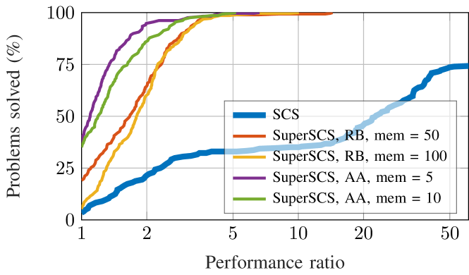
Figure 1: DM performance plot on 288 $\ell_{1}$-regularized PCA problems of the form (2s).

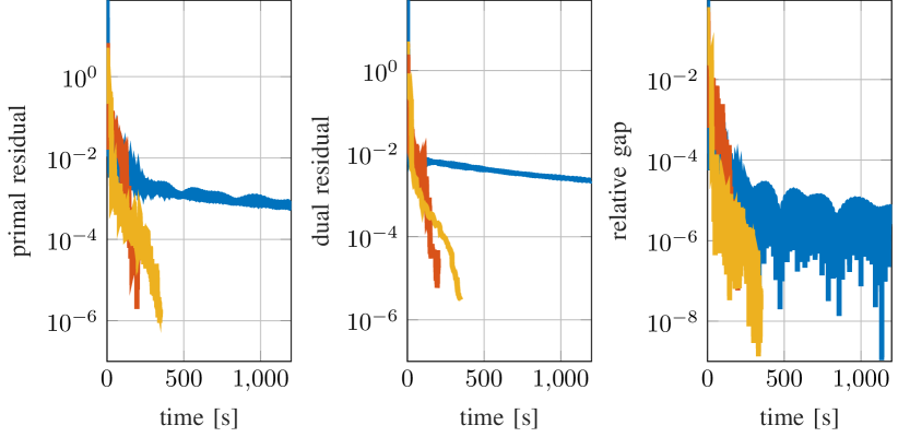
Figure 2: Progress of SuperSCS (with RB and AA directions) and SCS versus time for a large-scale SDP of the form (2s) with $d=500$ (with $m=625751$ and $n=250501$). [— SCS; — SuperSCS RB with memory 50; — SuperSCS AA with memory 5].

Additionally, for this benchmark we tried the interior-point solvers of SDPT3 [25] and Sedumi [23]. Both exhibited similar performance; in particular, for problems of dimension $Z\in\R^{140\times 140}$, SDPT3 and Sedumi required $6500\,\mathrm{s}$ to $7500\,\mathrm{s}$ and for problems of dimension $Z\in\R^{180\times 180}$ they required $19000\,\mathrm{s}$ to $21500\,\mathrm{s}$. Note that SuperSCS (with RB and memory 50) solves all problems in no more than $11.7\,\mathrm{s}$. Additionally, interior-point methods have an immense memory footprint of several GB, in this example whereas SuperSCS with RB and memory 100 needs as little as $211.1\,\mathrm{MB}$ and with AA and memory 5 consumes just $46.2\,\mathrm{MB}$.

V-C LASSO problems

Regularized least-squares problems with the $\|{}\cdot{}\|_{1}$-regularizer, also known as LASSO problems, are optimization problems of the form

$$\operatorname*{minimize}_{x\in\R^{n}}\nicefrac{{1}}{{2}}\|Ax-b\|^{2}+\mu\|x\|_{1},$$ (2z)

where $A\in\R^{m\times n}$ is a (sparse) matrix, and $\mu>0$ is the regularization weight. LASSO problems find applications in statistics and compressed sensing [22]. LASSO problems are cast as second-order cone programs [13].

TABLE II: LASSO: Solver Statistics

Method	$\operatorname{sgm}_{10}(t^{s})$	Success
SCS	5.97	100%
RB (mem:50)	2.88	100%
RB (mem:100)	2.61	100%
AA (mem:5)	3.38	100%
AA (mem:10)	3.87	100%

LASSO problems aim at finding a sparse vector $x$ which minimizes $\|Ax-b\|^{2}$. The sparseness of the minimizer $x^{\star}$ can be controlled by $\mu\in\{0.01,0.1,1\}$. We tested 1152 randomly generated LASSO problems with $n\in\{631,1000,1585,2512\}$, $m=\lceil n/5\rceil$, and matrices $A$ with condition numbers $\kappa_{A}\in\{10,215,4600,10^{5}\}$. The DM plot in Fig. 3 and the statistics presented in Table II demonstrate that SuperSCS, both with RB and AA directions, outperforms SCS.

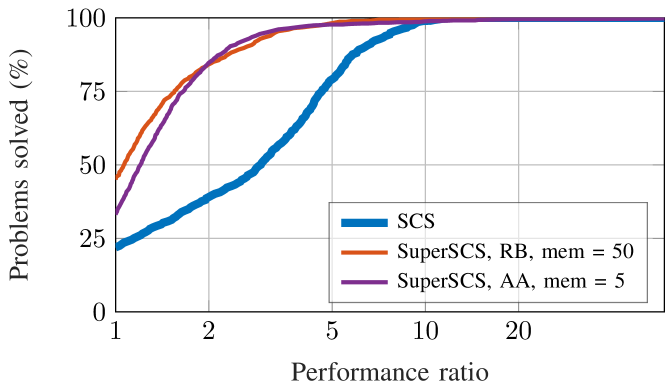
Figure 3: DM performance plot on 1152 LASSO problems.

V-D Sparse $\ell_{1}$-regularized logistic regression

Logistic regression is a regression model where dependent variables are binary [4]. The $\ell_{1}$ regularized variant of logistic regression aims at performing simultaneous regression and feature selection and amounts to solving an optimization problem of the following form [1]:

$$\operatorname*{minimize}_{w\in\R^{p}}\lambda\|w\|_{1}{}-{}\sum_{i=1}^{q}\log(1{}+{}\exp(a^{\top}w_{i}{}+{}b)).$$ (2ag)

Similar to LASSO (Sec. V-C), parameter $\lambda>0$ controls the sparseness of the solution $w^{\star}$. Such problems can be cast as conic programs with the exponential cone, which is not self-dual. A total of 288 randomly generated problems was used for benchmarking

TABLE III: Sparse $\ell_{1}$-regularized logistic regression: Solver Statistics

Method	$\operatorname{sgm}_{10}(t^{s})$	Success
SCS	4.85	100%
RB (mem:50)	7.23	100%
RB (mem:100)	7.28	100%
AA (mem:5)	3.00	100%
AA (mem:10)	3.09	100%

with $p\in\{80,100\}$, $q\in\{50,100,120\}$ and $\lambda\in\{10,20,50\}$. In Fig. 4 we observe that SuperSCS with RB directions is slower compared to SCS, however SuperSCS with AA is noticeably faster.

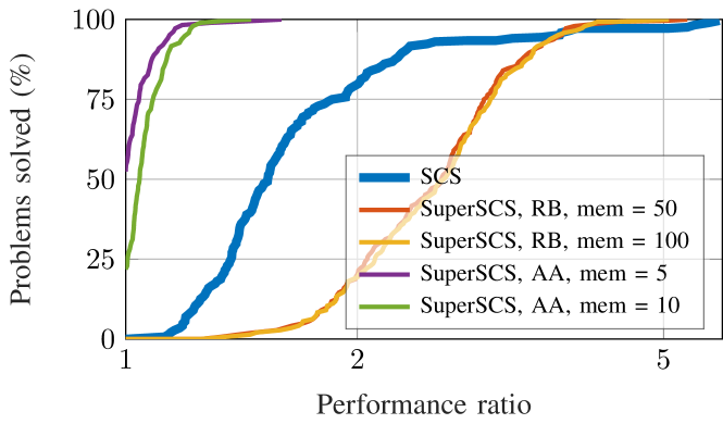
Figure 4: DM performance plot on 288 logistic regression problems of the form (2ag).

V-E Maros-Mészáros QP problems

TABLE IV: Maros-Mészáros QP problems: Solver Statistics

Method	$\operatorname{sgm}_{10}(t^{s})$	Success
SCS	56.61	83.02%
RB (mem:50)	9.66	90.57%
RB (mem:100)	6.57	90.57%
AA (mem:5)	5.79	90.57%
AA (mem:10)	8.62	91.51%

Here we present performance of SCS and SuperSCS (with RB and AA directions) on this collection of problems on the Maros-Mészáros collection of problems [15]. As shown in Fig. 5 SuperSCS, both with RB directions and Anderson’s acceleration, is faster and more robust compared to SCS. The two quasi-Newtonian directions appear to be on a par.

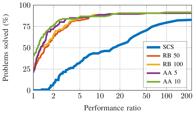
Figure 5: DM performance plot on the problems of the Maros-Mészáros repository.

VI Conclusions

In this work we introduced SuperSCS: a first-order method for large-scale conic optimization problems which combines the low iteration cost of SCS and the fast convergence of SuperMann. We have compared SuperSCS with SCS on a broad collection of conic optimization problems of practical interest. Using Dolan-Moré plots and runtime statistics, we demonstrated that SuperSCS with Anderson’s acceleration is faster and more robust than SCS.

The C implementation of SuperSCS builds up on SCS and is a free open-source software. SuperSCS can be interfaced from MATLAB, Python, can be invoked via CVX, CVXPy and YALMIP and is also available as a Docker image (see https://kul-forbes.github.io/scs/).

References

- [1] F. Abramovich and V. Grinshtein. High-dimensional classification by sparse logistic regression. ArXiv e-prints 1706.08344v2, 2017.
- [2] H.H. Bauschke and P.L. Combettes. Convex analysis and monotone operator theory in Hilbert spaces. Springer, 2011.
- [3] A. Ben-Tal and A. Nemirovski. Lectures on Modern Convex Optimization. SIAM, Jan 2001.
- [4] D.R. Cox. The regression analysis of binary sequences (with discussion). J Roy Stat Soc B, 20:215–242, 1958.
- [5] A. d’Aspremont, L. El Ghaoui, M.I. Jordan, and G.R.G. Lanckriet. A direct formulation for sparse PCA using semidefinite programming. SIAM Review, 49(3):434–448, Jan 2007.
- [6] S. Diamond and S. Boyd. CVXPY: A Python-embedded modeling language for convex optimization. J. Mach. Learn. Res., 17(83):1–5, 2016.
- [7] E.D. Dolan and J.J. Moré. Benchmarking optimization software with performance profiles. Math. Program., Ser. A, 91:201–213, 2002.
- [8] A. Domahidi, E. Chu, and S. Boyd. ECOS: An SOCP solver for embedded systems. In IEEE CDC, pages 3071–3076, 2013.
- [9] H. Fang and Y. Saad. Two classes of multisecant methods for nonlinear acceleration. Numer. Lin. Alg. Applic., 16(3):197–221, Mar 2009.
- [10] N. Gould and J. Scott. A note on performance profiles for benchmarking software. ACM Trans. Math. Software, 43(2):1–5, Aug 2016.
- [11] M. Grant and S. Boyd. CVX: Matlab software for disciplined convex programming, version 2.1. http://cvxr.com/cvx, Mar 2014.
- [12] J.B. Hiriart-Urruty and C. Lemaréchal. Fundamentals of convex analysis. Springer, 2004.
- [13] M. Sousa Lobo, L. Vandenberghe, S. Boyd, and H. Lebret. Applications of second-order cone programming. In ILAS Symp. Fast Alg. for Contr., Sign. Im. Proc., volume 284, pages 193–228, 1998.
- [14] J. Löfberg. YALMIP: A toolbox for modeling and optimization in MATLAB. In CACSD Conference, 2004.
- [15] I. Maros and C. Mészáros. A repository of convex quadratic programming problems. Optim. Meth. Soft., 11(1-4):671–681, Jan 1999.
- [16] H. Mitttelman. Decision tree for optimization problems: benchmarks for optimization software. http://plato.asu.edu/bench.html. [Online; accessed 1-June-2018].
- [17] MOSEK ApS. The MOSEK optimization toolbox for MATLAB manual. Version 8.1., 2017.
- [18] B. O’Donoghue, E. Chu, N. Parikh, and S. Boyd. Conic optimization via operator splitting and homogeneous self-dual embedding. JOTA, 169(3):1042–1068, Jun 2016.
- [19] B. O’Donoghue, E. Chu, N. Parikh, and S. Boyd. SCS: Splitting conic solver, v2.0.2. https://github.com/cvxgrp/scs, Nov 2017.
- [20] M. Powell. A hybrid method for nonlinear equations. Numerical Methods for Nonlinear Algebraic Equations, pages 87–144, 1970.
- [21] E.K. Ryu and S. Boyd. A primer on monotone operator methods: a survey. Appl. Comput. Math., 15(1):3–43, 2016.
- [22] P. Sopasakis, N. Freris, and P. Patrinos. Accelerated reconstruction of a compressively sampled data stream. In IEEE 24th European Signal Processing Conference EUSIPCO, pages 1078–1082, Aug 2016.
- [23] J.F. Sturm. Using SeDuMi 1.02, a MATLAB toolbox for optimization over symmetric cones. Optim. Meth. Soft., 11–12:625–653, 1999. Version 1.05 available at http://fewcal.kub.nl/sturm.
- [24] A. Themelis and P. Patrinos. Supermann: a superlinearly convergent algorithm for finding fixed points of nonexpansive operators. ArXiv e-prints 1609.06955, 2016.
- [25] R.H. Tütüncü, K. C. Toh, and M. J. Todd. Solving semidefinite-quadratic-linear programs using SDPT3. Math. Prog., 95(2):189–217, Feb 2003.
- [26] H.F. Walker and P. Ni. Anderson acceleration for fixed-point iterations. SIAM J. Numer. Anal., 49(4):1715–1735, Aug 2011.
- [27] Y. Ye, M. Todd, and S. Mizuno. An -iteration homogeneous and self-dual linear programming algorithm. Math. Oper. Res., 19(1):53–67, 1994.
- [28] Y. Zheng, G. Fantuzzi, A. Papachristodoulou, P. Goulart, and A. Wynn. Fast ADMM for homogeneous self-dual embedding of sparse SDPs. IFAC-PapersOnLine, 50(1):8411–8416, 2017.