Joint Antenna Array Mode Selection and User Assignment for Full-Duplex MU-MISO Systems

Abstract

This paper considers a full-duplex (FD) multiuser multiple-input single-output system where a base station simultaneously serves both uplink (UL) and downlink (DL) users on the same time-frequency resource. The crucial barriers in implementing FD systems reside in the residual self-interference and co-channel interference. To accelerate the use of FD radio in future wireless networks, we aim at managing the network interference more effectively by jointly designing the selection of half-array antenna modes (in the transmit or receive mode) at the BS with time phases and user assignments. The first problem of interest is to maximize the overall sum rate subject to quality-of-service requirements, which is formulated as a highly non-concave utility function followed by non-convex constraints. To address the design problem, we propose an iterative low-complexity algorithm by developing new inner approximations, and its convergence to a stationary point is guaranteed. To provide more insights into the solution of the proposed design, a general max-min rate optimization is further considered to maximize the minimum per-user rate while satisfying a given ratio between UL and DL rates. Furthermore, a robust algorithm is devised to verify that the proposed scheme works well under channel uncertainty. Simulation results demonstrate that the proposed algorithms exhibit fast convergence and substantially outperform existing schemes.

I Introduction

The rapid growth of the demand for high data rate in the next-generation communication systems requires innovative technologies that make the maximal use of radio spectrum. Even though advanced techniques such as multiple-input multiple-output (MIMO) antennas have been implemented to improve network throughput [2], half-duplex (HD) systems, where uplink (UL) and downlink (DL) communications are carried out orthogonally in time domain or in frequency domain, may not be able to provide sufficient improvements in the spectral efficiency (SE). Full-duplex (FD) communications, which allow for simultaneous UL and DL transmissions in the same time-frequency resource, theoretically double the SE when compared to HD. As a result, FD communications have been recognized as a promising technology for the forthcoming 5G wireless networks [3, 4, 5, 6].

Although the potential gains of FD can be easily foreseen, its major drawback is self-interference (SI) from the transmit (Tx) to receive (Rx) antennas at an FD wireless transceiver (e.g., a base station (BS)), which is typically much stronger than the signal of interest. Recently, there have been many efforts to develop analog and digital SI cancellation techniques to bring the SI power at the noise level when the Tx power is relatively low [7, 8, 9, 10, 11]. Such results have spurred research at the system level, considering small cell-based systems. In practice, complete elimination of the SI is not possible due to the limitations of hardware design [12, 13], and thus, recent works have considered FD systems under the effects of residual SI. Moreover, FD cellular networks also suffer from the user-to-user (UE-to-UE) interference caused by UL users to the ones in the DL channel, referred to as co-channel interference (CCI), which may become a performance bottleneck. The CCI is unavoidable in a cellular network, and it largely depends on the user position in the cell. While CCI was ignored in earlier FD designs [14], the latest research has taken it into account, especially in dense user-deployed small cell systems [15, 16, 17, 18, 19, 20, 21, 22, 23].

I-A Related Works

By considering both the residual SI and CCI, recent research has mainly focused on improving the SE [15, 16, 17, 18, 19, 20, 21, 22]. In [15] and [16], the sum rate (SR) maximization was studied in an FD system for both information and energy transfer. In [17], joint beamforming and power allocation were investigated to maximize the SE for a single-cell scenario.[18] further explored a multi-cell scenario, along with an additional quality-of-service (QoS) constraint. Under channel uncertainty, a robust design for the weighted SE optimization problem for a single-cell system was considered in [21]. In an FD multi-cell system, the weighted SE maximization problem was further examined in [19], while the authors in [22] focused on the user fairness design through a max-min problem for the SINRs of all users in the entire network. The performance of these systems degrades quickly as the residual SI and CCI increase, and to overcome this drawback, an approach integrating user grouping and time allocation was proposed in [20]. Nevertheless, the optimization under many slots of the communication time block (or the coherence time) results in an extremely high complexity, while the gain achieved from increasing the number of time slots suddenly decreases. If the SI and CCI become more severe, the system performance is still worse than the traditional HD scheme even with a large number of groups, since the full antenna array is not exploited in the transmission. Moreover, the number of binary variables to optimize the BS-user association scales exponentially with the number of DL and UL users.

Recently, a joint design of user assignment, power control and antenna selection has been applied to FD systems that further improves SE. In [24, 25, 26], the authors proposed an FD design based on user assignment, where users are assigned to one of the sub-carriers in an orthogonal frequency-division multiple access network. However, the improvement of such FD systems mainly relies on the frequency resource allocation, while the effect of SI still remains strong given that FD communication occurs in the same band. Regarding user assignment design, Ahn et al. in [27] proposed a user selection scheme where a set of users is selected to maximize the overall SR. The number of selected UL and DL users is assumed to be less than or equal to the number of receive (Rx) and transmit (Tx) antennas at the base station (BS), respectively. Regarding antenna selection techniques, they were studied in some simple FD end-to-end communications. For example, [28] considered an FD relaying system where two-antenna relays can switch their antenna modes (Tx and Rx) to improve the SE in forwarding the messages from the source to the destination. A point-to-point FD MIMO system was investigated in [29], in which Tx and Rx antennas are allowed to be active or not, to enhance the energy efficiency. More challengingly, in addition to the inherently present SI, FD multiuser systems also experience mutual interferences among users, and therefore, they should be considered in designing an FD system. Furthermore, a per-antenna selection causes high computational complexity, which motivates us to consider a half-array (HA) antenna selection in this work.

I-B Motivation and Contributions

Despite advancements made so far to SI cancellation, the residual SI still has a substantially negative impact on the system performance, and thus, needs to be mitigated. As evident from [17, 18, 19, 15, 20, 16], recent advanced FD designs may provide worse performance than HD when the residual SI becomes severe. Besides, as previously mentioned, there exists a small, but not negligible amount of CCI, especially when considering an FD system in a small cell scenario with UL and DL users in close proximity [17, 18]. Therefore, it is highly desirable to develop an efficient design that utilizes the same frequency resource for all users within one transmission time block while improving the SE. Moreover, the FD system should achieve at least the same performance as HD counterpart even in unexpected conditions.

In contrast with [15, 16, 17, 18, 19, 20], this paper considers a small cell FD system, which is enabled with an HA antenna mode selection and two-phase transmission. In particular, the transmission time block is split into two phases, and for each phase, two HAs of the antennas at the FD-enabled BS can be independently selected for UL and DL transmissions. By using this mode selection, our approach automatically switches among HD, conventional FD [17], two-phase FD [20], and even hybrid transmissions where the HD scheme (UL or DL transmission) is used in one phase and the FD scheme is applied in the other phase. Compared to the prior work, the proposed FD design has several advantages. Firstly, the proposed two-phase transmission helps better exploit the spatial degrees-of-freedom (DoF) since the number of users served at the same time is effectively reduced. Secondly, HA antenna selection supports the BS in finding better channel conditions and enabling the hybrid transmission. Moreover, by a joint design of the HA antenna mode selection and the two-phase transmission, we can achieve a better system performance, with the harmful effects of residual SI and CCI significantly reduced when compared with a typical FD cellular network [17, 18, 20, 19].

The advantages of the proposed FD design are paralleled with several challenges in the practical implementation. As the SI and CCI are strongly related to the performance of the DL and UL channels, it usually requires introducing integer variables to manage the BS-UE association. Consequently, the joint design problems of interest belong to the difficult class of mixed-integer non-convex problem, where both types of the binary and continuous variables are coupled to each other in the rate functions. In addition, the design problems are established in a blend of the UL (DL) channels and antenna selection variables, making the problems even more challenging. Furthermore, the acquisition of perfect channel state information (CSI), including the interference channels from the multiple users, is relatively unrealistic, and thus, the consideration of a joint robust FD transmission strategy becomes more critical. In this respect, a rigorous optimization and analysis are required to develop a low-complexity joint design.

Specifically, the main contributions of this paper are briefly described as follows:

1. We first propose a new FD transmission model in which two HAs at the BS are independently selected between the Rx and Tx modes in two phases of a time block. This model not only improves the achievable rate by selecting the modes for two HAs, but also mitigates effects of both residual SI and CCI by separating users into two phases. Interestingly, the new model can enable hybrid modes of the HD and FD to utilize a full-array antenna, which is not investigated in earlier works.

2. We formulate an SR maximization problem with QoS constraints under perfect CSI, which jointly optimizes HA mode selection, dynamically-timed phase, user assignment and power allocation. The design problem is a mixed-integer non-convex problem, and we present an iterative algorithm to solve it optimally in a centralized manner. In an effort to reduce the computational complexity, we first derive a set of subproblems without the integer constraints and tighten bounds for the constraints of subproblems. With the newly developed inner approximations, these subproblems can be efficiently solved via successive convex approximations. The optimal solution of the original problem is determined to correspond to the best optimal value of subproblems.

3. We further introduce a general max-min problem which aims at guaranteeing the achievable rate fairness. Although the objective function of this problem is not only non-concave but also non-smooth, the developments made to address the SR maximization problem are useful to obtain its solution.

4. For the imperfect CSI case, we consider a robust counterpart of the SR maximization problem when the errors are mainly due to estimation inaccuracies. We show that the worst-case robust SR maximization problem can be addressed in a similar manner as the SR maximization.

5. Numerical results show that the proposed algorithms have a fast convergence speed and outperform existing schemes. The new scheme is further shown to provide robustness against the estimation error under imperfect CSI.

I-C Paper Organization and Notation

The remainder of this paper is organized as follows. In Section II, we introduce the system model and formulate the design problem. The proposed algorithms for the SR maximization and max-min rate optimization are presented in Sections III and IV, respectively. In Section V, we study the robust FD transmission under uncertain channel information. Numerical results are presented in Section VI, and Section VII concludes the paper.

Notation: $\mathbf{X}^{T}$, $\mathbf{X}^{H}$ and ${\mathrm{tr}}(\mathbf{X})$ are the transpose, Hermitian transpose and trace of a matrix $\mathbf{X}$, respectively. $\left\langle\mathbf{x},\mathbf{y}\right\rangle={\mathrm{tr}}(\mathbf{x}^{H}\mathbf{y})$ denotes the inner product of vectors $\mathbf{x}$ and $\mathbf{y}$. $\|\cdot\|$ denotes the Euclidean norm of a matrix or vector, while $|\cdot|$ stands for the absolute value of a complex scalar. $\mathbb{E}[\cdot]$ denotes the statistical expectation and $\Re\{\cdot\}$ returns the real part of the argument. The notation $\mathbf{X}\succeq\mathbf{0}$ and $\mathbf{X}\succ\mathbf{0}$ represent that $\mathbf{X}$ is a positive-semidefinite and positive-definite matrix, respectively. $\mathbf{x}\preceq\mathbf{y}$ denotes the element-wise comparison of vectors, in which a certain element of $\mathbf{x}$ is not larger than the element of $\mathbf{y}$ at the same index. ${\mathrm{diag}}(\mathbf{x})$ stands for a diagonal matrix containing the elements of vector $\mathbf{x}$ as its main diagonal. $\mathbf{x}\sim\mathcal{CN}(\boldsymbol{\eta},\boldsymbol{Z})$ means that $\mathbf{x}$ is a random vector following a complex circularly symmetric Gaussian distribution with mean $\boldsymbol{\eta}$ and covariance matrix $\boldsymbol{Z}$. $\mathbf{dom}\;f$ stands for the domain of the function $f$. $\otimes$ is the Kronecker operator, while $\mathbf{and}$ and $\mathbf{nor}$ denote the and and negative or operations in Boolean algebra, respectively.

II Preliminaries

II-A System Model

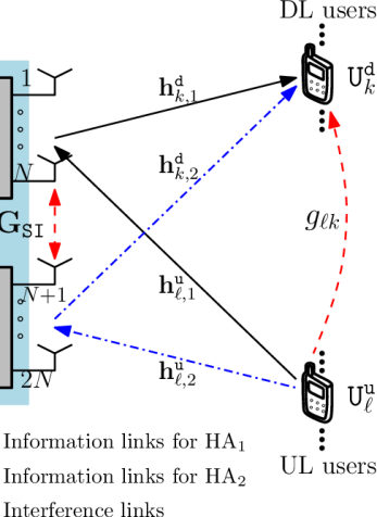
Figure 1: A small cell FD MU-MISO system. At the BS, HA₁ is from the $1$-st to the $N$-th antenna, while HA₂ is from the $(N+1)$-th to the $2N$-th antenna; at a certain moment, either one of the links from or to a HA is active, depending on the Tx/Rx-antenna modes (Rx mode for UL and Tx mode for DL).

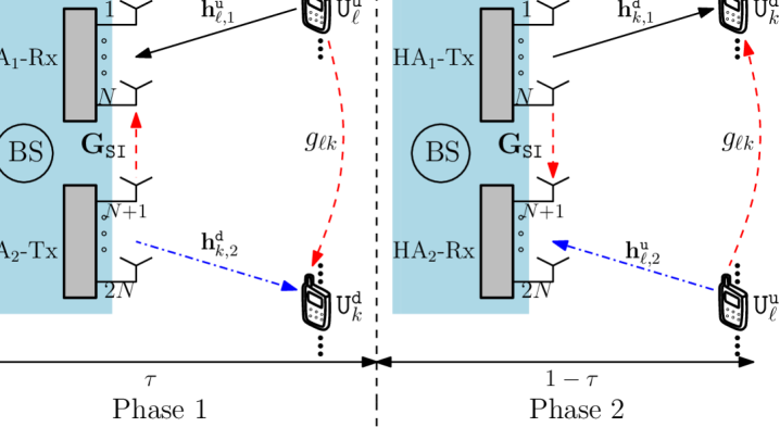
Figure 2: An example of two-phase transmission in the FD system. In Phase 1, HA₁ is set to the Rx mode, while HA₂ is set to the Tx mode, and vice versa in Phase 2. The links shown in the figure represent the active channels.

We consider a small cell FD multiuser multiple-input single-output (MU-MISO) system consisting of an FD-BS equipped with $2N$ antennas, $L$ single-antenna UL users, and $K$ single-antenna DL users, as illustrated in Fig. 2. We denote $\mathtt{U}_{\ell}^{\mathtt{u}},\;\forall\ell\in\mathcal{L}\triangleq\{1,2,\dots,L\}$ and $\mathtt{U}_{k}^{\mathtt{d}},\;\forall k\in\mathcal{K}\triangleq\{1,2,\dots,K\}$, the $\ell$-th UL and $k$-th DL user, respectively. The array of $2N$ antennas at the BS is split into two HAs of $N$ antennas: HA₁ from the $1$-st to the $N$-th antenna and HA₂ from the $(N+1)$-th to the $2N$-th antenna. Each HA can switch between Rx and Tx modes, corresponding to UL and DL, respectively. The channel vectors from $\mathtt{U}_{\ell}^{\mathtt{u}}$ to HA_i and from HA_i to $\mathtt{U}_{k}^{\mathtt{d}}$ are denoted by $\mathbf{h}_{\ell,i}^{\mathtt{u}}\in\mathbb{C}^{N\times 1}$ and $\mathbf{h}_{k,i}^{\mathtt{d}}\in\mathbb{C}^{N\times 1}$, respectively. At a certain time, the channels in Fig. 2 are either active or inactive, depending on the Tx/Rx mode selection for HA. The matrix $\mathbf{G}_{\mathtt{SI}}\in\mathbb{C}^{N\times N}$ represents the SI channel between HA₁ and HA₂, while $g_{\ell k}$ stands for the CCI channel from $\mathtt{U}_{\ell}^{\mathtt{u}}$ to $\mathtt{U}_{k}^{\mathtt{d}}$. The channel vectors capture the effects of both large- and small-scale fading.

We consider that the FD transmission takes place in two phases within each transmission time block, which is normalized to 1. Fig. 2 describes an example for the FD transmission in two phases, with transmission intervals of $\tau\text{ and }1-\tau\;(0<\tau<1)$, respectively. In the first phase, HA₁ and HA₂ are set to the Rx and Tx modes, respectively. Hence, $\mathbf{h}_{\ell,1}^{\mathtt{u}}$ and $\mathbf{h}_{k,2}^{\mathtt{d}}$ are active, while $\mathbf{h}_{k,1}^{\mathtt{d}}$ and $\mathbf{h}_{\ell,2}^{\mathtt{u}}$ are inactive. During the second phase, the Tx/Rx modes of the HAs are interchanged, i.e., $\mathbf{h}_{\ell,2}^{\mathtt{u}}$ and $\mathbf{h}_{k,1}^{\mathtt{d}}$ are active, while $\mathbf{h}_{k,2}^{\mathtt{d}}$ and $\mathbf{h}_{\ell,1}^{\mathtt{u}}$ are not. Herein, Fig. 2 illustrates one possible case to indicate that the HAs can be changed across two phases. The system model tends to exploit the channel conditions through the combination of the HA modes selection and two-phase transmission, resulting in three different transmission modes: FD, HD, and hybrid mode. In summary, the mode selection for HA_i in phase $j$ $(j=1,2)$ is optimized using the variables $\omega_{ij}\in\{0,1\}$, which form a binary matrix $\boldsymbol{\Omega}\in\mathbb{R}^{2\times 2}$ as

$$\boldsymbol{\Omega}=\begin{bmatrix}\omega_{11}&\omega_{12}\\ \omega_{21}&\omega_{22}\\ \end{bmatrix}\vspace{5pt}$$ (1)

where $\omega_{ij}=0$ or 1 indicates that HA_i in phase $j$ is set to the Rx mode (UL) or Tx mode (DL). We let the $j$-th column of $\boldsymbol{\Omega}$ be $\boldsymbol{\omega}_{j}$. Note that the HA modes in two phases depend on the entries of matrix $\boldsymbol{\Omega}$. Therefore, $\boldsymbol{\Omega}$ represents the transmission states of the system in one time block. Although (1) describes a model with a $2\times 2$ matrix, a scalable system can be enabled by changing the number of rows and/or that of columns of $\boldsymbol{\Omega}$ to create a general transmission model with multiple sub-array antennas and multiple time phases. However, solving the general case may not be suitable for practical implementations, as more RF chains and high complexity are required. Therefore, we consider the HA mode selection and two-phase transmission in the rest of the paper.

II-B Problem Formulation

In the DL transmission of phase $j$, the information signal $x_{k,j}^{\mathtt{d}}$, with $\mathbb{E}\bigl{[}|x_{k,j}^{\mathtt{d}}|^{2}\bigr{]}=1$, intended to $\mathtt{U}_{k}^{\mathtt{d}}$, is precoded using a beamforming vector $\mathbf{w}_{k,j}\in\mathbb{C}^{2N\times 1}$ at the BS. The signals received at the BS and $\mathtt{U}_{k}^{\mathtt{d}}$ in phase $j$ are, respectively, given as

$$\mathbf{y}_{j}^{\mathtt{u}} =\sum\nolimits_{\ell=1}^{L}p_{\ell,j}\boldsymbol{\bar{\Lambda}}_{j}\mathbf{h}_{\ell}^{\mathtt{u}}x_{\ell,j}^{\mathtt{u}}+\underbrace{\rho\sum\nolimits_{k=1}^{K}\mathbf{\bar{G}}_{\mathtt{SI}}^{H}\boldsymbol{\Lambda}_{j}\mathbf{w}_{k,j}x_{k,j}^{\mathtt{d}}}_{\text{SI}}+\mathbf{n}_{j},$$ (2)

$$y_{k,j}^{\mathtt{d}} =\sum\nolimits_{k^{\prime}=1}^{K}(\mathbf{h}_{k}^{\mathtt{d}})^{H}\boldsymbol{\Lambda}_{j}\mathbf{w}_{k^{\prime},j}x_{k^{\prime},j}^{\mathtt{d}}+\underbrace{\sum\nolimits_{\ell=1}^{L}p_{\ell,j}g_{\ell k}x_{\ell,j}^{\mathtt{u}}}_{\text{CCI}}+n_{k,j}$$ (3)

where $\mathbf{h}_{\ell}^{\mathtt{u}}\triangleq[(\mathbf{h}_{\ell,1}^{\mathtt{u}})^{H}\;(\mathbf{h}_{\ell,2}^{\mathtt{u}})^{H}]^{H}$ and $\mathbf{h}_{k}^{\mathtt{d}}\triangleq[(\mathbf{h}_{k,1}^{\mathtt{d}})^{H}\;(\mathbf{h}_{k,2}^{\mathtt{d}})^{H}]^{H}$. $\boldsymbol{\Lambda}_{j}$ and $\boldsymbol{\bar{\Lambda}}_{j}$ are diagonal matrices defined as $\boldsymbol{\Lambda}_{j}\triangleq{\mathrm{diag}}(\boldsymbol{\omega}_{j})\otimes\mathbf{I}_{N}$ and $\boldsymbol{\bar{\Lambda}}_{j}\triangleq{\mathrm{diag}}(\boldsymbol{\bar{\omega}}_{j})\otimes\mathbf{I}_{N}$, where $\boldsymbol{\bar{\omega}}_{j}$ is a bit-wise complement of the binary vector $\boldsymbol{\omega}_{j}$. $p_{\ell,j}^{2}\in\mathbb{R}$ and $x_{\ell,j}^{\mathtt{u}}$, with $\mathbb{E}\bigl{[}|x_{\ell,j}^{\mathtt{u}}|^{2}\bigr{]}=1$, are the UL transmit power and information signal from $\mathtt{U}_{\ell}^{\mathtt{u}}$ to BS in phase $j$, respectively. $n_{k,j}\sim\mathcal{CN}(0,\sigma_{k}^{2})$ and $\mathbf{n}_{j}\sim\mathcal{CN}(\mathbf{0},\sigma_{\mathtt{U}}^{2}\mathbf{I})$ represent the additive white Gaussian noise. The parameter $\rho\in\bigl{[}0,1\bigr{]}$ represents the degree of SI propagation [30], while the block anti-diagonal matrix $\mathbf{\bar{G}}_{\mathtt{SI}}$ is defined as $\mathbf{\bar{G}}_{\mathtt{SI}}=\left[\begin{smallmatrix}\mathbf{0}&\mathbf{G}_{\mathtt{SI}}\\ \mathbf{G}_{\mathtt{SI}}^{H}&\mathbf{0}\\ \end{smallmatrix}\right].$

Let $\mathbf{w}_{j}\triangleq\bigl{[}\mathbf{w}_{1,j}^{H}\;\mathbf{w}_{2,j}^{H}\cdots\mathbf{w}_{K,j}^{H}\bigr{]}^{H}\in\mathbb{C}^{2NK\times 1}$ and $\mathbf{p}_{j}\triangleq\bigl{[}p_{1,j}\;p_{2,j}\cdots p_{L,j}\bigr{]}^{H}\in\mathbb{C}^{L\times 1}$. By using minimum mean square error and successive interference cancellation (MMSE-SIC) decoder [31], the signal-to-interference-plus-noise ratio (SINR) of $\mathtt{U}_{\ell}^{\mathtt{u}}$ at the BS in phase $j$ can be written as

$$\gamma_{\ell}^{\mathtt{u}}\bigl{(}\boldsymbol{\omega}_{j},\mathbf{w}_{j},\mathbf{p}_{j}\bigr{)}=p_{\ell,j}^{2}(\mathbf{\tilde{h}}_{\ell,j}^{\mathtt{u}})^{H}\boldsymbol{\Psi}_{\ell,j}^{-1}\mathbf{\tilde{h}}_{\ell,j}^{\mathtt{u}}$$ (4)

where

$$\boldsymbol{\Psi}_{\ell,j}\triangleq\sum\nolimits_{\ell^{\prime}=\ell+1}^{L}p_{\ell^{\prime},j}^{2}\mathbf{\tilde{h}}_{\ell^{\prime},j}^{\mathtt{u}}(\mathbf{\tilde{h}}_{\ell^{\prime},j}^{\mathtt{u}})^{H}+\rho^{2}\sum\nolimits_{k=1}^{K}\mathbf{\tilde{G}}_{j}^{H}\mathbf{w}_{k,j}\mathbf{w}_{k,j}^{H}\mathbf{\tilde{G}}_{j}+\sigma_{\mathtt{U}}^{2}\mathbf{I},$$

and $\mathbf{\tilde{h}}_{\ell,j}^{\mathtt{u}}\triangleq\boldsymbol{\bar{\Lambda}}_{j}\mathbf{h}_{\ell}^{\mathtt{u}}$ and $\mathbf{\tilde{G}}_{j}\triangleq\boldsymbol{\Lambda}_{j}\mathbf{\bar{G}}_{\mathtt{SI}}$ are the effective UL and residual SI channels, respectively. Next, we can express the received SINR of $\mathtt{U}_{k}^{\mathtt{d}}$ in phase $j$ as

$$\gamma_{k}^{\mathtt{d}}\bigl{(}\boldsymbol{\omega}_{j},\mathbf{w}_{j},\mathbf{p}_{j}\bigr{)}=\frac{\bigl{|}(\mathbf{\tilde{h}}_{k,j}^{\mathtt{d}})^{H}\mathbf{w}_{k,j}\bigr{|}^{2}}{\psi_{k,j}}$$ (5)

where

$$\psi_{k,j}\triangleq\sum\nolimits_{k^{\prime}=1,k^{\prime}\neq k}^{K}\bigl{|}\bigl{(}\mathbf{\tilde{h}}_{k,j}^{\mathtt{d}}\bigr{)}^{H}\mathbf{w}_{k^{\prime},j}\bigr{|}^{2}+\sum\nolimits_{\ell=1}^{L}p_{\ell,j}^{2}|g_{\ell k}|^{2}+\sigma_{k}^{2},$$

and $\mathbf{\tilde{h}}_{k,j}^{\mathtt{d}}\triangleq\boldsymbol{\Lambda}_{j}\mathbf{h}_{k}^{\mathtt{d}}$ is the effective channel for $\mathtt{U}_{k}^{\mathtt{d}}$.

Remark 1

It is clear that the SINRs in (4) and (5) can express all possible cases of $\boldsymbol{\Omega}$. Remarkably, the SINR is separately computed for each phase, depending on the columns of matrix $\boldsymbol{\Omega}$, i.e., $\boldsymbol{\omega}_{j}$. If the FD mode is selected, half of the effective channel vector is active corresponding to the HA mode in $\boldsymbol{\omega}_{j}$. The HD mode is selected when both HAs are set to either Rx or Tx. When both HAs are in Rx mode (or Tx mode), the full vector of the effective UL channel in (4) (or effective DL channel in (5)) is active, while the DL SINRs in (5) (or the UL SINRs in (4)) are equal to 0 due to the full vector of the DL effective channel (or the effective UL channel) being off.

From (4) and (5), the achievable rates (nats/s/Hz) of $\mathtt{U}_{\ell}^{\mathtt{u}}$ and $\mathtt{U}_{k}^{\mathtt{d}}$ in one transmission time block are, respectively, expressed as

$$R_{\ell}^{\mathtt{u}}\bigl{(}\boldsymbol{\Omega},\mathbf{w},\mathbf{P},\tau,\boldsymbol{\alpha}_{\ell}^{\mathtt{u}}\bigr{)} =\sum_{j=1}^{2}\alpha_{\ell,j}^{\mathtt{u}}\bar{\tau}_{j}\ln\bigl{(}1+\gamma_{\ell}^{\mathtt{u}}(\boldsymbol{\omega}_{j},\mathbf{w}_{j},\mathbf{p}_{j})\bigr{)},$$ (6)

$$R_{k}^{\mathtt{d}}\bigl{(}\boldsymbol{\Omega},\mathbf{w},\mathbf{P},\tau,\boldsymbol{\alpha}_{k}^{\mathtt{d}}\bigr{)} =\sum_{j=1}^{2}\alpha_{k,j}^{\mathtt{d}}\bar{\tau}_{j}\ln\bigl{(}1+\gamma_{k}^{\mathtt{d}}(\boldsymbol{\omega}_{j},\mathbf{w}_{j},\mathbf{p}_{j})\bigr{)}$$ (7)

where $\mathbf{w}\triangleq[\mathbf{w}_{1}^{H}\;\mathbf{w}_{2}^{H}]^{H}$ and $\mathbf{P}\triangleq[\mathbf{p}_{1}\;\mathbf{p}_{2}]$. The new binary variables $\boldsymbol{\alpha}_{\ell}^{\mathtt{u}}\triangleq[\alpha_{\ell,1}^{\mathtt{u}}\;\alpha_{\ell,2}^{\mathtt{u}}],\;\forall\ell\in\mathcal{L}$ and $\boldsymbol{\alpha}_{k}^{\mathtt{d}}\triangleq[\alpha_{k,1}^{\mathtt{d}}\;\alpha_{k,2}^{\mathtt{d}}],\forall k\in\mathcal{K}$ are used for user assignments, and they indicate whether $\mathtt{U}_{\ell}^{\mathtt{u}}$ and $\mathtt{U}_{k}^{\mathtt{d}}$ are respectively served by the BS in phase $j$. If they are, $\alpha_{\ell,j}^{\mathtt{u}}$ and $\alpha_{k,j}^{\mathtt{d}}$ are set to 1; otherwise, $\alpha_{\ell,j}^{\mathtt{u}}$ and $\alpha_{k,j}^{\mathtt{d}}$ are equal to 0. The communication time is defined as $\bar{\tau}_{j}\triangleq(2-j)\tau+(j-1)(1-\tau)$, ensuring that phases 1 and 2 are within $\tau$ and $(1-\tau)$, respectively.

We consider a general objective function, denoted as $\mathcal{R}\bigl{(}\{R_{\ell}^{\mathtt{u}}\},\{R_{k}^{\mathtt{d}}\}\bigr{)}$. For simplicity, $R_{\ell}^{\mathtt{u}}$ and $R_{k}^{\mathtt{d}}$ are used to represent $R_{\ell}^{\mathtt{u}}\bigl{(}\boldsymbol{\Omega},\mathbf{w},\mathbf{P},\tau,\boldsymbol{\alpha}_{\ell}^{\mathtt{u}}\bigr{)}$ and $R_{k}^{\mathtt{d}}\bigl{(}\boldsymbol{\Omega},\mathbf{w},\mathbf{P},\tau,\boldsymbol{\alpha}_{k}^{\mathtt{d}}\bigr{)}$ given in (6) and (7), respectively. In particular, a joint design problem is mathematically formulated as

$$\underset{\boldsymbol{\Omega},\mathbf{w},\mathbf{P},\tau,\boldsymbol{\alpha}_{\ell}^{\mathtt{u}},\boldsymbol{\alpha}_{k}^{\mathtt{d}}}{\text{maximize}} \quad\mathcal{R}\bigl{(}\{R_{\ell}^{\mathtt{u}}\},\{R_{k}^{\mathtt{d}}\}\bigr{)}$$ (8a)

subject to $$\quad\omega_{ij}\in\{0,1\},\forall i,j=1,2,$$ (8b)

$$\quad 1\leq\sum\nolimits_{i=1}^{2}\sum\nolimits_{j=1}^{2}\omega_{ij}\leq 3,$$ (8c)

$$\quad\sum\nolimits_{j=1}^{2}\bar{\tau}_{j}p_{\ell,j}^{2}\leq P_{\ell}^{\text{max}},\;\forall\ell\in\mathcal{L},$$ (8d)

$$\quad p_{\ell,j}^{2}\leq P_{\ell}^{\infty},\;\forall\ell\in\mathcal{L},j=1,2,$$ (8e)

$$\quad p_{\ell,j}\geq 0,\;\forall\ell\in\mathcal{L},j=1,2,$$ (8f)

$$\quad\sum\nolimits_{j=1}^{2}\bar{\tau}_{j}\|\mathbf{w}_{j}\|^{2}\leq P_{t}^{\text{max}},$$ (8g)

$$\quad\|\mathbf{w}_{j}\|^{2}\leq P_{t}^{\infty},\;j=1,2,$$ (8h)

$$\quad 0<\tau<1,$$ (8i)

$$\quad\alpha_{\ell,j}^{\mathtt{u}},\;\alpha_{k,j}^{\mathtt{d}}\in\{0,1\},\;\forall\ell\in\mathcal{L},\forall k\in\mathcal{K},j=1,2.$$ (8j)

Constraints (8b) and (8c) are the mode selections of HAs, in which constraint (8c) guarantees that UL and DL transmissions are executed at least in one phase. In fact, when the summation in (8c) is equal to 2, the system operates in either FD or HD mode. If this summation equals 1 or 3, the hybrid mode is activated. Constraints (8d) and (8g) cap the maximum transmit power of $\mathtt{U}_{\ell}^{\mathtt{u}}$ and BS, respectively. As in [20, 23], the coupling between communication time $\bar{\tau}_{j}$ and transmit power in (8d) and (8g) indicates that the transmit power in one phase is associated with its interval and independent of the other phase, under the condition that the total transmit power does not exceed the power budgets, $P_{\ell}^{\text{max}}$ at $\mathtt{U}_{\ell}^{\mathtt{u}}$ and $P_{t}^{\text{max}}$ at the BS. The physical constraints (8e) and (8h) are imposed to ensure that it is not possible to transmit an arbitrary high power at every instant. Herein, $P_{\ell}^{\infty}$ and $P_{t}^{\infty}$ represent the maximum transmit power per phase at $\mathtt{U}_{\ell}^{\mathtt{u}}$ and at the BS, respectively. Without loss of generality, we choose $P_{\ell}^{\infty}\equiv P_{\ell}^{\text{max}}$ and $P_{t}^{\infty}\equiv P_{t}^{\text{max}}$. Finally, constraints (8j) are associated with the users’ assignments in each phase. Through problem (8), the SI and CCI are significantly reduced since the proposed two-phase scheme allows the system to serve its users in various transmission time $\bar{\tau}_{j}$, i.e., one of two phases or the whole transmission block. In addition, the HA modes are dynamically selected in the optimization, and thus, this scheme can easily switch to FD scheme; or asymmetric HD scheme where the UL and DL transmissions independently operating in two phases of one time block can occupy different time intervals; or hybrid mode where FD is used in one phase, and HD using full antenna array for either uplink (UL) or downlink (DL) transmission is employed in the other phase.

Remark 2

Based on problem (8), the modes for HAs are dynamically selected to maximize the objective function (i.e., SR or max-min rate). Moreover, the FD-enabled system can be switched to HD transmission if the SI and CCI become strong. Therefore, the HD mode case corresponds to one of those cases that are generated by HA modes in two phases. When the HD mode case is selected, the full-antenna array ($2N$ antennas) is used in each phase for UL or DL transmission while the SI and CCI automatically disappear due to the joint optimization of HA mode selection and power allocation.

III Proposed Algorithm for Sum Rate Maximization

In this section, we investigate the following joint design problem for SR maximization:

$$\underset{\boldsymbol{\Omega},\mathbf{w},\mathbf{P},\tau,\boldsymbol{\alpha}_{\ell}^{\mathtt{u}},\boldsymbol{\alpha}_{k}^{\mathtt{d}}}{\text{maximize}} \quad R_{\Sigma}\triangleq\sum\nolimits_{\ell=1}^{L}R_{\ell}^{\mathtt{u}}+\sum\nolimits_{k=1}^{K}R_{k}^{\mathtt{d}}$$ (9a)

subject to $$\quad\eqref{eq: prob. general form b}-\eqref{eq: prob. general form j},$$ (9b)

$$\quad R_{\ell}^{\mathtt{u}}\geq\bar{R}_{\ell}^{\mathtt{u}},\forall\ell\in\mathcal{L},$$ (9c)

$$\quad R_{k}^{\mathtt{d}}\geq\bar{R}_{k}^{\mathtt{d}},\forall k\in\mathcal{K}$$ (9d)

where the objective function $\mathcal{R}\bigl{(}\{R_{\ell}^{\mathtt{u}}\},\{R_{k}^{\mathtt{d}}\}\bigr{)}$ in (8) is replaced by $R_{\Sigma}=\sum\nolimits_{\ell\in\mathcal{L}}R_{\ell}^{\mathtt{u}}+\sum\nolimits_{k\in\mathcal{K}}R_{k}^{\mathtt{d}}$. $\bar{R}_{\ell}^{\mathtt{u}}\geq 0$ in (9c) and $\bar{R}_{k}^{\mathtt{d}}\geq 0$ in (9d) specify the minimum rate requirements for $\mathtt{U}_{\ell}^{\mathtt{u}}$ and $\mathtt{U}_{k}^{\mathtt{d}}$, respectively. It is clear that problem (9) is a mixed-integer non-convex programming, which is an NP-hard problem [32]. In addition, the binary variables $(\boldsymbol{\Omega},\boldsymbol{\alpha}_{\ell}^{\mathtt{u}},\boldsymbol{\alpha}_{k}^{\mathtt{d}})$ and the continuous variables $(\mathbf{w},\mathbf{P},\tau)$ are strongly coupled, making the design problem even more challenging. In what follows, we develop an efficient successive algorithm with low complexity to solve problem (9). Specifically, we first decouple the original problem (9) into subproblems of lower dimensions, and then use a bound-tightening process to further relieve the computational complexity. Although each subproblem is still non-convex, we iteratively approximate each subproblem by a sequence of convex programs based on the inner approximation method [33], for which an iterative algorithm is then proposed.

III-A Subproblems for Problem (9)

Since the complexity of the BS-UE association will increase exponentially with the number of users, it is not practical to seek all possible BS-UE combinations. In particular, the number of possible cases for two HAs is the product of $4^{2}$ cases for the HA mode selection, $2^{2L}$ for UL and $2^{2K}$ for DL users assignments. To overcome this issue, we first utilize the symmetry property of problem (9) to deal with the binary variables $\boldsymbol{\Omega}$ in (8b) and (8c) by introducing the following proposition.

Proposition 1

A finite set is defined as $\mathcal{B}\triangleq\{\mathrm{b}`b_{1}b_{0}|b_{0},b_{1}\in\{0,1\}\}$, where $\mathrm{b}`b_{1}b_{0}$ denotes a binary number with two bits including the most significant bit, $b_{1}$, and the least significant bit, $b_{0}$. Then, we consider a function $f_{\omega}$ as

$$f_{\omega}: \;\{0,1\}^{2\times 1}\rightarrow\mathcal{B},$$

$$\qquad\mathbf{z}\quad\;\;\rightarrow\hat{z},\;f_{\omega}(\mathbf{z})=\mathrm{b}`z_{1}z_{2}.$$ (10)

From $f_{\omega}$ in (1), a mapping is established as

$$g_{\omega}: \;\{0,1\}^{2\times 1}\times\{0,1\}^{2\times 1}\rightarrow\mathcal{B}\times\mathcal{B},$$

$$\quad\boldsymbol{\Omega}=\boldsymbol{\omega}_{1}\times\boldsymbol{\omega}_{2}\quad\quad\;\rightarrow\quad\boldsymbol{\hat{\omega}},\;g_{\omega}(\boldsymbol{\Omega})=[f_{\omega}(\boldsymbol{\omega}_{1})\;f_{\omega}(\boldsymbol{\omega}_{2})].$$

We define a lexicographically ordered set as

$$\mathcal{B}^{\prime}\triangleq\{\boldsymbol{\hat{\omega}}=[\hat{\omega}_{1}\;\hat{\omega}_{2}]\;|\;\hat{\omega}_{1}<\hat{\omega}_{2}\;\vee\;\hat{\omega}_{1}=\hat{\omega}_{2}\notin\{\mathrm{b}`00,\mathrm{b}`11\}\}\subset\mathcal{B}\times\mathcal{B}.$$ (11)

Without loss of optimality, problem (9) can be decoupled into subproblems without constraints (8b) and (8c) by fixing $\boldsymbol{\Omega}$, such that $\boldsymbol{\Omega}\in\mathcal{S}_{\boldsymbol{\Omega}}=g_{\omega}^{-1}(\mathcal{B}^{\prime})$.  ∎

Proof:

Please see Appendix A. ∎

Remark 3

Since $\hat{\omega}_{j}$’s are binary numbers, the inequality $\hat{\omega}_{1}\leq\hat{\omega}_{2}$ is not equivalent to $\boldsymbol{\omega}_{1}\preceq\boldsymbol{\omega}_{2}$. Therefore, $(\hat{\omega}_{1},\hat{\omega}_{2})$ must be searched in the area of $\mathcal{S}_{\hat{\omega}}$ to find all possible cases of HA modes. Then, the corresponding argument $(\boldsymbol{\omega}_{1},\boldsymbol{\omega}_{2})$ obtained via the inverse of $g_{\omega}$ is applied to problem (9) to derive a subproblem without the binary matrix variable $\boldsymbol{\Omega}$.

Remark 4

It is realized that $\mathcal{S}_{\hat{\omega}}$ can be considered as an ordered set where a lexicographical order is applied to pairs of phases $(\hat{\omega}_{1},\hat{\omega}_{2})$. This has two advantages: (i) it requires to partly search for the optimal solution, instead of all symmetric regions; (ii) without loss of generality, the property of lexicographical order is very useful to extend pairs of two phases to a sequence of multiple phases, while the HA mode selection is easily transformed into multiple sub-array antennas selection by replacing the set $\mathcal{B}$ with $\mathcal{B}_{n}\triangleq\{\mathrm{b}`b_{n-1}\dots b_{0}|b_{0},b_{1},\dots,b_{n-1}\in\{0,1\}\}$.

Next, we deal with the binary nature of ($\boldsymbol{\alpha}_{\ell}^{\mathtt{u}},\boldsymbol{\alpha}_{k}^{\mathtt{d}}$) in (8j). For $\boldsymbol{\alpha}\triangleq\bigl{[}[\boldsymbol{\alpha}_{\ell}^{\mathtt{u}}]_{\ell\in\mathcal{L}}^{H}\;[\boldsymbol{\alpha}_{k}^{\mathtt{d}}]_{k\in\mathcal{K}}^{H}\bigr{]}$ and $\mathbf{R}\triangleq[\mathbf{r}_{\mathtt{u}}^{H}\;\mathbf{r}_{\mathtt{d}}^{H}]^{H}$, with $\mathbf{r}_{\mathtt{u}}=\bigl{[}\bar{\tau}_{1}\ln\bigl{(}1+\gamma_{\ell}^{\mathtt{u}}(\mathbf{w}_{1},\mathbf{p}_{1},\boldsymbol{\omega}_{1})\bigl{)}$ $\bar{\tau}_{2}\ln\bigl{(}1+\gamma_{\ell}^{\mathtt{u}}(\mathbf{w}_{2},\mathbf{p}_{2},\boldsymbol{\omega}_{2})\bigr{)}\bigr{]}_{\ell\in\mathcal{L}}$ and $\mathbf{r}_{\mathtt{d}}=\bigl{[}\bar{\tau}_{1}\ln\bigl{(}1+\gamma_{k}^{\mathtt{d}}(\mathbf{w}_{1},\mathbf{p}_{1},\boldsymbol{\omega}_{1})\bigr{)}\;\bar{\tau}_{2}\ln\bigl{(}1+\gamma_{k}^{\mathtt{d}}(\mathbf{w}_{2},\mathbf{p}_{2},\boldsymbol{\omega}_{2})\bigr{)}\bigr{]}_{k\in\mathcal{K}}$, the SR is ${\mathrm{tr}}(\boldsymbol{\alpha}\mathbf{R})$. Since each element of $\mathbf{R}$ is greater than zero, the SR is maximized if all entries of $\boldsymbol{\alpha}$ are set to 1. Therefore, fixing $\alpha_{\ell,j}^{\mathtt{u}}$ and $\alpha_{k,j}^{\mathtt{d}}$ to 1 always provides an upper bound for an arbitrary feasible point. In other words, we assume an optimal solution with some $\alpha_{\ell,j}^{\mathtt{u}}=0$ and $\alpha_{k,j}^{\mathtt{d}}=0,\;\ell\in\mathcal{L},k\in\mathcal{K},j=1,2$, denoted by $\mathbf{X}^{*}=\{\boldsymbol{\Omega}^{*},\mathbf{w}^{*},\mathbf{P}^{*},\tau^{*},(\boldsymbol{\alpha}_{\ell}^{\mathtt{u}})^{*},(\boldsymbol{\alpha}_{k}^{\mathtt{d}})^{*}|\;\text{some }\alpha_{\ell,j}^{\mathtt{u}}=0\;\&\;\alpha_{k,j}^{\mathtt{d}}=0\}$. Let $\mathbf{X}^{*}|_{\alpha=1}$ be $\mathbf{X}^{*}$ with the values of all $\alpha_{\ell,j}^{\mathtt{u}}$ and $\alpha_{k,j}^{\mathtt{d}}$ replaced by 1. It is realized that $\mathbf{X}^{*}|_{\alpha=1}$ is also an optimal solution for (9), since the objective function value given by $\mathbf{\hat{X}}|_{\alpha=1}$ is always equal to or larger than that given by $\mathbf{\hat{X}}$, where $\mathbf{\hat{X}}$ is an arbitrary feasible point, and $\mathbf{\hat{X}}|_{\alpha=1}$ is $\mathbf{\hat{X}}$ with the values of all $\alpha_{\ell,j}^{\mathtt{u}}$ and $\alpha_{k,j}^{\mathtt{d}}$ replaced by 1. Intuitively, the user assignment variables aim to effectively switch users on-off, and thus direct computation of the values of user assignment variables as in [20, 24] is unnecessary and results in high complexity. As a result, we can consider the constraint (8j) in problem (9) as feasibility by fixing $\alpha_{\ell,j}^{\mathtt{u}}$ and $\alpha_{k,j}^{\mathtt{d}}$ to 1 at the beginning of the optimization, and removing them from problem (9). After solving problem (9), an expression for two cases is used for user assignments as

$$\alpha_{\ell,j}^{\mathtt{u}}{(\text{or }\alpha_{k,j}^{\mathtt{d}})}=\begin{cases}1,&\text{if }\gamma_{\ell,j}^{\mathtt{u},(*)}{(\text{or }\gamma_{k,j}^{\mathtt{d},(*)})}\geq\gamma_{\varepsilon},\\ 0,&\text{otherwise}\end{cases}$$ (12)

where $\gamma_{\ell,j}^{\mathtt{u}}$ and $\gamma_{k,j}^{\mathtt{d}}$ merely represent $\gamma_{\ell}^{\mathtt{u}}\bigl{(}\boldsymbol{\omega}_{j},\mathbf{w}_{j},\mathbf{p}_{j}\bigr{)}$ and $\gamma_{k}^{\mathtt{d}}\bigl{(}\boldsymbol{\omega}_{j},\mathbf{w}_{j},\mathbf{p}_{j}\bigr{)}$, respectively. $\gamma_{\varepsilon}$ is a threshold defined such that if the obtained SINR optimal values, $\gamma_{\ell,j}^{\mathtt{u},(*)}{(\text{or }\gamma_{k,j}^{\mathtt{d},(*)})}$, $\forall\ell\in\mathcal{L},\forall k\in\mathcal{K},j=1,2$, are lower than $\gamma_{\varepsilon}$, they are small enough to be negligible and thus $\alpha_{\ell,j}^{\mathtt{u}}{(\text{or }\alpha_{k,j}^{\mathtt{d}})}$ is set to 0.

By fixing ($\boldsymbol{\Omega}$, $\boldsymbol{\alpha}_{\ell}^{\mathtt{u}}$, $\boldsymbol{\alpha}_{k}^{\mathtt{d}}$) as previously discussed, the achievable rates for $\mathtt{U}_{\ell}^{\mathtt{u}}$ and $\mathtt{U}_{k}^{\mathtt{d}}$ are equivalently expressed as $R_{\ell}^{\mathtt{u}}\bigl{(}\mathbf{w},\mathbf{P},\tau|\boldsymbol{\Omega}\bigr{)}=\sum\nolimits_{j=1}^{2}\bar{\tau}_{j}\ln\bigl{(}1+\gamma_{\ell}^{\mathtt{u}}(\mathbf{w}_{j},\mathbf{p}_{j}|\boldsymbol{\omega}_{j})\bigr{)}$ and $R_{k}^{\mathtt{d}}\bigl{(}\mathbf{w},\mathbf{P},\tau|\boldsymbol{\Omega}\bigr{)}=\sum\nolimits_{j=1}^{2}\bar{\tau}_{j}\ln\bigl{(}1+\gamma_{k}^{\mathtt{d}}(\mathbf{w}_{j},\mathbf{p}_{j}|\boldsymbol{\omega}_{j})\bigr{)}$. For a given value of $\boldsymbol{\Omega}\in\mathcal{S}_{\boldsymbol{\Omega}}$, problem (9) can be decoupled into the following subproblems:

$$\underset{\mathbf{w},\mathbf{P},\tau}{\text{maximize}} \quad\sum\nolimits_{\ell=1}^{L}R_{\ell}^{\mathtt{u}}\bigl{(}\mathbf{w},\mathbf{P},\tau|\boldsymbol{\Omega}\bigr{)}+\sum\nolimits_{k=1}^{K}R_{k}^{\mathtt{d}}\bigl{(}\mathbf{w},\mathbf{P},\tau|\boldsymbol{\Omega}\bigr{)},\qquad$$ (13a)

subject to $$\quad\eqref{eq: prob. general form d}-\eqref{eq: prob. general form i},$$ (13b)

$$\quad R_{\ell}^{\mathtt{u}}\bigl{(}\mathbf{w},\mathbf{P},\tau|\boldsymbol{\Omega}\bigr{)}\geq\bar{R}_{\ell}^{\mathtt{u}},\;\forall\ell\in\mathcal{L},$$ (13c)

$$\quad R_{k}^{\mathtt{d}}\bigl{(}\mathbf{w},\mathbf{P},\tau|\boldsymbol{\Omega}\bigr{)}\geq\bar{R}_{k}^{\mathtt{d}},\;\forall k\in\mathcal{K}.$$ (13d)

III-B Bound Tightening for Power Constraints

We now exploit the properties of HA selection to tighten bounds for power constraints {(8d), (8e), (8g), (8h)}, so that the search region containing the optimal solution is downsized significantly. For instance, if a certain HA is set to Rx, its effective channel to all DL users is obviously inactive. Intuitively, the corresponding beamforming vector can be arbitrarily chosen in a restricted region while holding the optimality. Therefore, the following lemma is derived to limit the search region as it dynamically tightens the bounds for power constraints.

Lemma 1

Let $\mathbf{w}_{k,i,j}$ be the $i$-th half of beamforming vector $\mathbf{w}_{k,j}$. For a subproblem with $\omega_{ij}\;(i,j=1,2)$ being set to 0, $\mathbf{w}_{k,i,j}$ can be fixed at a certain value without any effect on the optimal value.  ∎

Proof:

Please see Appendix B. ∎

Using Lemma 1, we can tighten the bound of $\mathbf{w}_{k,i,j}$ to reduce the search region when $\omega_{ij}=0$. To preserve the optimal value, the feasible set for other beamforming vectors needs to be kept as large as possible, meaning that $\|\mathbf{w}_{k,i,j}^{*}\|^{2}=0$. For further analysis, we consider the viewpoint that the beamforming is transmitted in one phase, i.e., switching to the HD mode. In the case of the proposed model, the power budget $P_{t}^{\text{max}}$ is issued within one time interval of the transmission block. Meanwhile, a traditional HD system switches between UL and DL modes, and each mode occupies one transmission block, meaning that $P_{t}^{\text{max}}$ is issued for every two transmission blocks (UL and DL). To make it general, the upper bound of the beamforming vectors in the proposed scheme is tightened through the time scale. In particular, for $\chi_{j}\triangleq\omega_{1j}\;\mathbf{nor}\;\omega_{2j},j=1,2$, the DL power constraints (8g) and (8h) can be rewritten as

$$\sum\nolimits_{j=1}^{2}\tau_{j}^{\mathtt{d}}\|\mathbf{w}_{j}\|^{2} \leq P_{t}^{\text{max}},$$ (14a)

$$\sum\nolimits_{k=1}^{K}\|\mathbf{w}_{k,i,j}\|^{2} \leq P_{t}^{\infty}\omega_{ij},\;i,j=1,2$$ (14b)

where $\tau_{j}^{\mathtt{d}}\triangleq\bar{\tau}_{j}+\chi_{3-j}\bar{\tau}_{3-j},j=1,2$. It is clear that $\|\mathbf{w}_{k,i,j}\|^{2}$ is automatically upper bounded by 0 when $\omega_{ij}=0$, and the number of variables for the beamforming vector is thus reduced to half per phase. Similarly, the power constraints for $\mathtt{U}_{\ell}^{\mathtt{u}}$ in (8d) and (8e) can be expressed as

$$\sum\nolimits_{j=1}^{2}\tau_{j}^{\mathtt{u}}p_{\ell,j}^{2}\leq P_{\ell}^{\text{max}},\;\forall\ell\in\mathcal{L},$$ (15a)

$$p_{\ell,j}^{2}\leq P_{\ell}^{\infty}\bar{\beta}_{j},\;\forall\ell\in\mathcal{L},j=1,2$$ (15b)

where $\tau_{j}^{\mathtt{u}}\triangleq\bar{\tau}_{j}+\beta_{3-j}\bar{\tau}_{3-j},j=1,2$, with $\beta_{j}\triangleq\omega_{1j}\;\mathbf{and}\;\omega_{2j},$ and $\bar{\beta}_{j}$ is the bit complement of $\beta_{j}$.

Remark 5

The power allocation for UL users is upper bounded by 0 only if both HAs are switched to the Tx mode. Therefore, constraints (15b) use $\bar{\beta}_{j}$ on the right-hand side (RHS), instead of $\omega_{ij}$ in (14b). With the appearance of $\beta_{j}$ and $\chi_{j}$, the HD-switching mode achieves at least the sum rate of the traditional HD system because the proposed method can dynamically set the transmission time for $\tau_{j}^{\mathtt{u}}$ and $\tau_{j}^{\mathtt{d}}$ under given values of $\beta_{j}$ and $\chi_{j}$, while the traditional HD system sets the same interval for both UL and DL.

Finally, subproblem (13) is reformulated as

$$\underset{\mathbf{w},\mathbf{P},\tau}{\text{maximize}} \quad\sum\nolimits_{\ell=1}^{L}R_{\ell}^{\mathtt{u}}\bigl{(}\mathbf{w},\mathbf{P},\tau|\boldsymbol{\Omega}\bigr{)}+\sum\nolimits_{k=1}^{K}R_{k}^{\mathtt{d}}\bigl{(}\mathbf{w},\mathbf{P},\tau|\boldsymbol{\Omega}\bigr{)},\qquad$$ (16a)

subject to $$\quad\eqref{eq: prob. general form f},\eqref{eq: prob. general form i},\eqref{eq: prob. max sum SE 1 c},\eqref{eq: prob. max sum SE 1 d},\eqref{eq: DL power constraints},\eqref{eq: UL power constraints}.$$ (16b)

For subproblem (16) at hand, the power allocation for the optimization in $(\mathbf{w},\mathbf{P},\tau)$ still remains highly non-convex. Specifically, the objective (16a) is a non-concave function while constraints (13c), (13d), (14a) and (15a) are non-convex.

III-C Proposed Convex Approximation-based Iterative Algorithm

Herein, we will solve subproblem (16) via a sequence of convex programs that provides the minorant solution. As in [34], a function $\tilde{h}$ is a convex majorant (or concave minorant, respectively) of a function $h$ at a point $\bar{x}\in\mathbf{dom}\;h$ iff $\tilde{h}(\bar{x})=h(\bar{x})$ and $\tilde{h}(x)\geq h(x)$ (or $\tilde{h}(x)\leq h(x)$, respectively), $\forall x\in\mathbf{dom}\;h$. According to this definition, subproblem (16) can be convexified as follows.

Let us start by introducing the alternative variables $\mu_{j},j=1,2$ as

$$\bar{\tau}_{2} = 1/\mu_{2},$$ (17)

$$\bar{\tau}_{1} = 1-1/\mu_{2}\geq 1/\mu_{1}.\vspace{-5pt}$$ (18)

For $0<\bar{\tau}_{j}<1$, the following additional linear and convex constraints are imposed:

$$\mu_{j}>1,j=1,2,$$ (19)

$$1/\mu_{1}+1/\mu_{2}\leq 1$$ . (20)

To handle the non-concave function $R_{\ell}^{\mathtt{u}}\bigl{(}\mathbf{w},\mathbf{P},\tau|\boldsymbol{\Omega}\bigr{)}$ in (16a), we can generally examine $R_{\ell,j}^{\mathtt{u}}(\mathbf{w}_{j},\mathbf{p}_{j},\mu_{j})\triangleq\frac{1}{\mu_{j}}\ln\bigl{(}1+\gamma_{\ell}^{\mathtt{u}}\bigl{(}\mathbf{w}_{j},\mathbf{p}_{j}|\boldsymbol{\omega}_{j}\bigr{)}\bigr{)}$ instead of $\bar{\tau}_{j}\ln\bigl{(}1+\gamma_{\ell}^{\mathtt{u}}\bigl{(}\mathbf{w}_{j},\mathbf{p}_{j}|\boldsymbol{\omega}_{j}\bigr{)}\bigr{)}$. By the Schur complement, the epigraph of $\gamma_{\ell}^{\mathtt{u}}\bigl{(}\mathbf{w}_{j},\mathbf{p}_{j}|\boldsymbol{\omega}_{j}\bigr{)}$ can be expressed with a linear matrix inequality [35]. In the spirit of [15], at a feasible point $(\mathbf{w}_{j}^{(\kappa)},\mathbf{p}_{j}^{(\kappa)},\mu_{j}^{(\kappa)})$ found at iteration $\kappa$ of the proposed iterative algorithm, a concave quadratic minorant of $R_{\ell,j}^{\mathtt{u}}(\mathbf{w}_{j},\mathbf{p}_{j},\mu_{j})$, denoted by $\mathcal{R}_{\ell,j}^{\mathtt{u},(\kappa)}$, is

$$R_{\ell,j}^{\mathtt{u}}(\mathbf{w}_{j},\mathbf{p}_{j},\mu_{j})\geq-\varpi(z_{\ell,j}^{(\kappa)},\mu_{j}^{(\kappa)})\mu_{j}+\zeta(z_{\ell,j}^{(\kappa)},\mu_{j}^{(\kappa)})-\frac{\varphi_{\ell}^{(\kappa)}(\mathbf{w}_{j},\mathbf{p}_{j}|\boldsymbol{\omega}_{j})}{\mu_{j}^{(\kappa)}}+\frac{2z_{\ell,j}^{(\kappa)}}{\mu_{j}^{(\kappa)}p_{\ell,j}^{(\kappa)}}p_{\ell,j}:=\mathcal{R}_{\ell,j}^{\mathtt{u},(\kappa)}\qquad$$ (21)

where

$$z_{\ell,j}^{(\kappa)}\triangleq\gamma_{\ell}^{\mathtt{u}}(\mathbf{w}_{j}^{(\kappa)},\mathbf{p}_{j}^{(\kappa)}|\boldsymbol{\omega}_{j}),\;\varpi(z_{\ell,j}^{(\kappa)},\mu_{j}^{(\kappa)})\triangleq\frac{\ln\bigl{(}1+z_{\ell,j}^{(\kappa)}\bigr{)}}{(\mu_{j}^{(\kappa)})^{2}},\;\zeta(z_{\ell,j}^{(\kappa)},\mu_{j}^{(\kappa)})\triangleq\frac{2\ln\bigl{(}1+z_{\ell,j}^{(\kappa)}\bigr{)}-z_{\ell,j}^{(\kappa)}}{\mu_{j}^{(\kappa)}},$$

$$\varphi_{\ell}^{(\kappa)}(\mathbf{w}_{j},\mathbf{p}_{j}|\boldsymbol{\omega}_{j})\triangleq\displaystyle{\mathrm{tr}}\Bigl{(}\bigl{(}p_{\ell,j}^{2}\mathbf{\tilde{h}}_{\ell,j}^{\mathtt{u}}(\mathbf{\tilde{h}}_{\ell,j}^{\mathtt{u}})^{H}+\boldsymbol{\Psi}_{\ell,j}\bigl{)}\bigl{(}(\boldsymbol{\Psi}_{\ell,j}^{(\kappa)})^{-1}-(\boldsymbol{\Psi}_{(\ell-1),j}^{(\kappa)})^{-1}\bigr{)}\Bigr{)},$$

$$\boldsymbol{\Psi}_{\ell,j}^{(\kappa)}\triangleq\sum\nolimits_{\ell^{\prime}=\ell+1}^{L}\bigl{(}p_{\ell^{\prime},j}^{(\kappa)}\bigr{)}^{2}\mathbf{\tilde{h}}_{\ell^{\prime},j}^{\mathtt{u}}\bigl{(}\mathbf{\tilde{h}}_{\ell^{\prime},j}^{\mathtt{u}}\bigr{)}^{H}+\rho^{2}\sum\nolimits_{k=1}^{K}\mathbf{\tilde{G}}_{j}^{H}\mathbf{w}_{k,j}^{(\kappa)}\bigl{(}\mathbf{w}_{k,j}^{(\kappa)}\bigr{)}^{H}\mathbf{\tilde{G}}_{j}+\sigma_{\mathtt{U}}^{2}\mathbf{I}.$$

Next, we address the non-concave function $R_{k}^{\mathtt{d}}\bigl{(}\mathbf{w},\mathbf{P},\tau|\boldsymbol{\Omega}\bigr{)}$. For $R_{k,j}^{\mathtt{d}}(\mathbf{w}_{j},\mathbf{p}_{j},$ $\mu_{j})\triangleq\frac{1}{\mu_{j}}\ln\bigl{(}1+\gamma_{k}^{\mathtt{d}}(\mathbf{w}_{j},\mathbf{p}_{j}|\boldsymbol{\omega}_{j})\bigr{)}$, it follows that

$$R_{k,j}^{\mathtt{d}}(\mathbf{w}_{j},\mathbf{p}_{j},\mu_{j})\geq\frac{1}{\mu_{j}}\ln\bigl{(}1+\frac{1}{\vartheta_{k,j}}\bigr{)}$$ (22)

which imposes the following constraints.

$$\gamma_{k}^{\mathtt{d}}(\mathbf{w}_{j},\mathbf{p}_{j}|\boldsymbol{\omega}_{j})\geq\frac{1}{\vartheta_{k,j}}\;\forall k\in\mathcal{K},\;j=1,2,$$ (23a)

$$\vartheta_{k,j}>0,\;\forall k\in\mathcal{K},\;j=1,2$$ (23b)

where $\vartheta_{k,j}$ are newly introduced variables. Note that constraint (23a) will hold with equality at optimum leading to the equality of (22). In addition, constraint (23a) is convexified as

$$\psi_{k,j}\leq\vartheta_{k,j}\gamma_{\text{s}}^{(\kappa)}\bigl{(}\mathbf{w}_{k,j}\bigr{)},\;\forall k\in\mathcal{K},\;j=1,2$$ (24)

over the trust region

$$\gamma_{\text{s}}^{(\kappa)}(\mathbf{w}_{k,j})\triangleq 2\Re\{(\mathbf{\tilde{h}}_{k,j}^{\mathtt{d}})^{H}\mathbf{w}_{k,j}^{(\kappa)}\}\Re\{(\mathbf{\tilde{h}}_{k,j}^{\mathtt{d}})^{H}\mathbf{w}_{k,j}\}-\bigl{(}\Re\{(\mathbf{\tilde{h}}_{k,j}^{\mathtt{d}})^{H}\mathbf{w}_{k,j}^{(\kappa)}\}\bigr{)}^{2}>0,\;\forall k,j$$ (25)

where $|(\mathbf{\tilde{h}}_{k,j}^{\mathtt{d}})^{H}\mathbf{w}_{k,j}|^{2}$ is innerly approximated by $\gamma_{\text{s}}^{(\kappa)}(\mathbf{w}_{k,j})$ due to its convexity [15]. It can be seen that constraint (24) is convex and also admits the second-order cone (SOC) representation. Furthermore, the concave minorant of $R_{k,j}^{\mathtt{d}}(\mathbf{w}_{j},\mathbf{p}_{j},$ $\mu_{j})$ in (22) at the $(\kappa+1)$-th iteration, denoted by $\mathcal{R}_{k,j}^{\mathtt{d},(\kappa)}$, is found as

$$R_{k,j}^{\mathtt{d}}(\mathbf{w}_{j},\mathbf{p}_{j},\mu_{j}) \geq\nu(\vartheta_{k,j}^{(\kappa)},\mu_{j}^{(\kappa)})+\xi(\vartheta_{k,j}^{(\kappa)},\mu_{j}^{(\kappa)})\vartheta_{k,j}+\lambda(\vartheta_{k,j}^{(\kappa)},\mu_{j}^{(\kappa)})\mu_{j}:=\mathcal{R}_{k,j}^{\mathtt{d},(\kappa)}$$ (26)

where $\nu(\vartheta_{k,j}^{(\kappa)},\mu_{j}^{(\kappa)})$, $\xi(\vartheta_{k,j}^{(\kappa)},\mu_{j}^{(\kappa)})$ and $\lambda(\vartheta_{k,j}^{(\kappa)},\mu_{j}^{(\kappa)})$ are respectively defined as

$$\nu(\vartheta_{k,j}^{(\kappa)},\mu_{j}^{(\kappa)}) \triangleq\frac{2}{\mu_{j}^{(\kappa)}}\ln\Bigl{(}1+\frac{1}{\vartheta_{k,j}^{(\kappa)}}\Bigr{)}+\frac{1}{\bigl{(}\vartheta_{k,j}^{(\kappa)}+1\bigr{)}\mu_{j}^{(\kappa)}},\quad\xi(\vartheta_{k,j}^{(\kappa)},\mu_{j}^{(\kappa)})\triangleq-\frac{1}{\vartheta_{k,j}^{(\kappa)}\bigl{(}\vartheta_{k,j}^{(\kappa)}+1\bigr{)}\mu_{j}^{(\kappa)}},$$

$$\lambda(\vartheta_{k,j}^{(\kappa)},\mu_{j}^{(\kappa)}) \triangleq-\frac{1}{\bigl{(}\mu_{j}^{(\kappa)}\bigr{)}^{2}}\ln\Bigl{(}1+\frac{1}{\vartheta_{k,j}^{(\kappa)}}\Bigr{)}.$$

Obviously, we can iteratively replace $R_{\ell}^{\mathtt{u}}\bigl{(}\mathbf{w},\mathbf{P},\tau|\boldsymbol{\Omega}\bigr{)}$ and $R_{k}^{\mathtt{d}}\bigl{(}\mathbf{w},\mathbf{P},\tau|\boldsymbol{\Omega}\bigr{)}$ by $\sum_{j=1}^{2}\mathcal{R}_{\ell,j}^{\mathtt{u},(\kappa)}$ and $\sum_{j=1}^{2}\mathcal{R}_{k,j}^{\mathtt{d},(\kappa)}$ to arrive at the convex constraints for (13c) and (13d), respectively.

Finally, let us convexify the power constraints (14a) and (15a). By substituting (17) into (14a) and (15a), we obtain two new constraints as

$$\mathcal{T}_{1}(\chi_{2})\|\mathbf{w}_{1}\|^{2}+\mathcal{T}_{2}(\chi_{1})\|\mathbf{w}_{2}\|^{2}\leq P_{t}^{\text{max}}+f_{\text{c}}^{d}\bigl{(}\mathbf{w},\mu_{2}\bigr{)},$$ (27a)

$$\mathcal{T}_{1}(\beta_{2})p_{\ell,1}^{2}+\mathcal{T}_{2}(\beta_{1})p_{\ell,2}^{2}\leq P_{\ell}^{\text{max}}+f_{\text{c}}^{u}\bigl{(}\mathbf{\hat{p}}_{\ell},\mu_{2}\bigr{)},\;\forall\ell\in\mathcal{L}$$ (27b)

where $\mathcal{T}_{1}(x)=\bigl{(}1+\frac{x}{\mu_{2}}\bigr{)}$ and $\mathcal{T}_{2}(x)=\bigl{(}\frac{1}{\mu_{2}}+x\bigr{)}$, while $\chi_{j}$ and $\beta_{j}$, $j=1,2$ are constant, depending on a fixed value of $\boldsymbol{\Omega}$. We define $f_{\text{c}}^{d}\bigl{(}\mathbf{w},\mu_{2}\bigr{)}\triangleq\frac{1}{\mu_{2}}\|\mathbf{w}_{1}\|^{2}+\frac{\chi_{1}}{\mu_{2}}\|\mathbf{w}_{2}\|^{2}$ and $f_{\text{c}}^{u}\bigl{(}\mathbf{\hat{p}}_{\ell},\mu_{2}\bigr{)}\triangleq\frac{1}{\mu_{2}}p_{\ell,1}^{2}+\frac{\beta_{1}}{\mu_{2}}p_{\ell,2}^{2}$, where $\mathbf{\hat{p}}_{\ell}\in\mathbb{R}^{2\times 1}$ is the transpose of the $\ell$-th row of $\mathbf{P}$. We remark that both left-hand sides of (27) are convex while their RHSs are quadratic-over-linear functions. By applying the first-order approximation to $f_{\text{c}}^{d}\bigl{(}\mathbf{w},\mu_{2}\bigr{)}$ around the point $(\mathbf{w}^{(\kappa)},\mu_{2}^{(\kappa)}\bigr{)}$ and $f_{\text{c}}^{u}\bigl{(}\mathbf{\hat{p}}_{\ell},\mu_{2}\bigr{)}$ around the point $\bigl{(}\mathbf{\hat{p}}_{\ell}^{(\kappa)},\mu_{2}^{(\kappa)}\bigr{)}$, the functions $f_{\text{c}}^{d}\bigl{(}\mathbf{w},\mu_{2}\bigr{)}$ and $f_{\text{c}}^{u}\bigl{(}\mathbf{\hat{p}}_{\ell},\mu_{2}\bigr{)}$ are innerly approximated as

$$f_{\text{c}}^{d}\bigl{(}\mathbf{w},\mu_{2}\bigr{)} \geq f_{\text{c}}^{d}\bigl{(}\mathbf{w}^{(\kappa)},\mu_{2}^{(\kappa)}\bigr{)}+\Bigl{<}\nabla f_{\text{c}}^{d}\bigl{(}\mathbf{w}^{(\kappa)},\mu_{2}^{(\kappa)}\bigr{)},\bigl{(}\mathbf{w},\mu_{2}\bigr{)}-\bigl{(}\mathbf{w}^{(\kappa)},\mu_{2}^{(\kappa)}\bigr{)}\Bigr{>}$$

$$=2\frac{\Re\{\bigl{(}\mathbf{w}_{1}^{(\kappa)}\bigr{)}^{H}\mathbf{w}_{1}\}}{\mu_{2}^{(\kappa)}}+2\frac{\chi_{1}\Re\{\bigl{(}\mathbf{w}_{2}^{(\kappa)}\bigr{)}^{H}\mathbf{w}_{2}\}}{\mu_{2}^{(\kappa)}}-\frac{f_{\text{c}}^{d}\bigl{(}\mathbf{w}^{(\kappa)},\mu_{2}^{(\kappa)}\bigr{)}}{\mu_{2}^{(\kappa)}}\mu_{2}$$

$$:=\hat{f}_{\text{c}}^{d,(\kappa)}\bigl{(}\mathbf{w},\mu_{2}\bigr{)}$$ (28a)

$$f_{\text{c}}^{u}\bigl{(}\mathbf{\hat{p}}_{\ell},\mu_{2}\bigr{)} \geq f_{\text{c}}^{u}\bigl{(}\mathbf{\hat{p}}_{\ell}^{(\kappa)},\mu_{2}^{(\kappa)}\bigr{)}+\Bigl{<}\nabla f_{\text{c}}^{u}\bigl{(}\mathbf{\hat{p}}_{\ell}^{(\kappa)},\mu_{2}^{(\kappa)}\bigr{)},\bigl{(}\mathbf{\hat{p}}_{\ell},\mu_{2}\bigr{)}-\bigl{(}\mathbf{\hat{p}}_{\ell}^{(\kappa)},\mu_{2}^{(\kappa)}\bigr{)}\Bigr{>}$$

$$=2\frac{p_{\ell,1}^{(\kappa)}}{\mu_{2}^{(\kappa)}}p_{\ell,1}+2\frac{\beta_{1}p_{\ell,2}^{(\kappa)}}{\mu_{2}^{(\kappa)}}p_{\ell,2}-\frac{f_{\text{c}}^{u}\bigl{(}\mathbf{\hat{p}}_{\ell}^{(\kappa)},\mu_{2}^{(\kappa)}\bigr{)}}{\mu_{2}^{(\kappa)}}\mu_{2}:=\hat{f}_{\text{c}}^{u,(\kappa)}\bigl{(}\mathbf{\hat{p}}_{\ell},\mu_{2}\bigr{)}.$$ (28b)

As a result, the convex constraints for (27) read as

$$\mathcal{T}_{1}(\chi_{2})\|\mathbf{w}_{1}\|^{2}+\mathcal{T}_{2}(\chi_{1})\|\mathbf{w}_{2}\|^{2}\leq P_{t}^{\text{max}}+\hat{f}_{\text{c}}^{d,(\kappa)}\bigl{(}\mathbf{w},\mu_{2}\bigr{)},$$ (29a)

$$\mathcal{T}_{1}(\beta_{2})p_{\ell,1}^{2}+\mathcal{T}_{2}(\beta_{1})p_{\ell,2}^{2}\leq P_{\ell}^{\text{max}}+\hat{f}_{\text{c}}^{u,(\kappa)}\bigl{(}\mathbf{\hat{p}}_{\ell},\mu_{2}\bigr{)}.$$ (29b)

In summary, the convex program providing a minorant maximization for (16) solved at iteration $(\kappa+1)$ of the proposed algorithm is given by

$$\underset{\mathbf{w},\mathbf{P},\boldsymbol{\mu},\boldsymbol{\vartheta}}{\text{maximize}} \quad\mathcal{R}_{\Sigma}^{(\kappa+1)}\triangleq\sum\nolimits_{\ell=1}^{L}\sum\nolimits_{j=1}^{2}\mathcal{R}_{\ell,j}^{\mathtt{u},(\kappa)}+\sum\nolimits_{k=1}^{K}\sum\nolimits_{j=1}^{2}\mathcal{R}_{k,j}^{\mathtt{d},(\kappa)}$$ (30a)

subject to $$\quad\eqref{eq: prob. general form f},\eqref{eq: DL power constraints b},\eqref{eq: UL power constraints b},\eqref{eq: alternative var. constraint 1},\eqref{eq: alternative var. constraint 2},\eqref{eq: positive vartheta constraint},\eqref{eq: vartheta constraints},\eqref{eq: positive effective channel constraint},\eqref{eq: power constraints approx. - altered variables},$$ (30b)

$$\quad\sum\nolimits_{j=1}^{2}\mathcal{R}_{\ell,j}^{\mathtt{u},(\kappa)}\geq\bar{R}_{\ell}^{\mathtt{u}},\forall\ell\in\mathcal{L},$$ (30c)

$$\quad\sum\nolimits_{j=1}^{2}\mathcal{R}_{k,j}^{\mathtt{d},(\kappa)}\geq\bar{R}_{k}^{\mathtt{d}},\forall k\in\mathcal{K}$$ (30d)

where $\boldsymbol{\mu}\triangleq[\mu_{1}\;\mu_{2}]$ and $\boldsymbol{\vartheta}\triangleq[\vartheta_{k,j}]_{k\in\mathcal{K},j=1,2}$. Note that the convex program (30) can be efficiently solved per iteration by existing solvers (e.g., MOSEK [36] or SeDuMi [37]) and the optimal solution for (16) is one of eight cases of $\boldsymbol{\Omega}$ in (1). By comparing the eight optimal values of subproblems, the global solution $\bigl{(}\boldsymbol{\Omega}^{*},\mathbf{W}^{*},\mathbf{P}^{*},\tau^{*}\bigr{)}$ for (9) is derived, and it corresponds to the maximum among eight optimal values. The proposed iterative algorithm for solving problem (9) is briefly described in Algorithm 1.

1:  Initialization: Set $\mathcal{R}_{\text{SR}}^{\max}:=-\infty$, $\varepsilon:=10^{-3}$, $\gamma_{\varepsilon}:=10^{-3}$, $\boldsymbol{\alpha}_{\ell}^{\mathtt{u}}=\boldsymbol{\alpha}_{k}^{\mathtt{d}}:=\mathbf{1}$, and $\bigl{(}\boldsymbol{\Omega}^{*},\mathbf{w}^{*},\mathbf{P}^{*},\tau^{*}\bigr{)}$$:=\mathbf{0}$.

2:  for each $\boldsymbol{\Omega}\in\mathcal{S}_{\boldsymbol{\Omega}}$ do {solving subproblem (16)}

3:     Generating an initial point: Set $\kappa:=0$ and solve (31) to generate $(\mathbf{w}^{(0)},\mathbf{P}^{(0)},\boldsymbol{\mu}^{(0)},\boldsymbol{\vartheta}^{(0)})$.

4:     repeat

5:        Solve (30) to obtain $\bigl{(}\mathbf{w}^{\star},\mathbf{P}^{\star},\boldsymbol{\mu}^{\star},\boldsymbol{\vartheta}^{\star}\bigr{)}$ and $\mathcal{R}_{\Sigma}^{(\kappa+1)}$.

6:        Update $(\mathbf{w}^{(\kappa+1)},\mathbf{P}^{(\kappa+1)},\boldsymbol{\mu}^{(\kappa+1)},\boldsymbol{\vartheta}^{(\kappa+1)}):=(\mathbf{w}^{\star},\mathbf{P}^{\star},\boldsymbol{\mu}^{\star},\boldsymbol{\vartheta}^{\star}$).

7:        Set $\kappa:=\kappa+1$.

8:     until Convergence

9:     if $\mathcal{R}_{\Sigma}^{(\kappa)}>\mathcal{R}_{\text{SR}}^{\max}$ then {if true, then there exists a better solution for (9)}

10:        Update $\mathcal{R}_{\text{SR}}^{\max}:=\mathcal{R}_{\Sigma}^{(\kappa)}$ and $\bigl{(}\boldsymbol{\Omega}^{*},\mathbf{w}^{*},\mathbf{P}^{*},\tau^{*}\bigr{)}:=\bigl{(}\boldsymbol{\Omega},\mathbf{w}^{(\kappa)},\mathbf{P}^{(\kappa)},(1-1/\mu_{2}^{(\kappa)})\bigr{)}$.

11:        Update $\boldsymbol{\alpha}_{\ell}^{\mathtt{u}}$ and $\boldsymbol{\alpha}_{k}^{\mathtt{d}}$ as in (12), and $R_{\Sigma}$ in (9a).

12:     end if

13:  end for

Algorithm 1 Proposed Iterative Algorithm for the SR Maximization Problem (9)

Generating an initial feasible point: To execute the loop for solving (16), Algorithm 1 needs to initialize a feasible point $(\mathbf{w}^{(0)},\mathbf{P}^{(0)},\boldsymbol{\mu}^{(0)},\boldsymbol{\vartheta}^{(0)})$ by consecutively solving a simpler problem as

$$\underset{\mathbf{w},\mathbf{P},\boldsymbol{\mu},\boldsymbol{\vartheta},\varrho}{\text{maximize}} \quad\varrho$$ (31a)

subject to $$\quad\eqref{eq: prob. max sum SE 2 b},$$ (31b)

$$\quad\sum\nolimits_{j=1}^{2}\mathcal{R}_{\ell,j}^{\mathtt{u},(\kappa)}-\bar{R}_{\ell}^{\mathtt{u}}\geq\varrho,\forall\ell\in\mathcal{L},$$ (31c)

$$\quad\sum\nolimits_{j=1}^{2}\mathcal{R}_{k,j}^{\mathtt{d},(\kappa)}-\bar{R}_{k}^{\mathtt{d}}\geq\varrho,\forall k\in\mathcal{K}$$ (31d)

where $\varrho$ is a new variable. The goal of solving (31) is not to focus on maximizing $\varrho$, but rather to find a feasible point for (30). Simply, the break condition for generating a starting point in (31) is $\varrho>0$.

Convergence analysis: As in [35], the proposed algorithm obtains the optimal point satisfying the Karush-Kuhn-Tucker (KKT) conditions or KKT-invexity. In fact, since Algorithm 1 is based on the inner approximation, it is true that for the sequence of convex programs in (30) every point in a feasible set $\mathcal{F}^{(\kappa)}$ of the considered problem at iteration $\kappa$ is also feasible for the problem at iteration $(\kappa+1)$, i.e., $\mathcal{F}^{(\kappa+1)}\supseteq\mathcal{F}^{(\kappa)}$ [33]. This means that $\mathcal{F}^{(\kappa)},\forall\kappa$, is considered as a convex subset in the order topology, and thus the set $\mathcal{F}^{(\kappa)}$ is connected [38]. According to [39], it satisfies the KKT-invex condition when $\kappa\rightarrow\infty$. As a result, the optimal solution of this sequence is monotonically improved toward the KKT point. For the practical implementation, Algorithm 1 terminates upon reaching $\mathcal{R}_{\Sigma}^{(\kappa+1)}-\mathcal{R}_{\Sigma}^{(\kappa)}<\varepsilon$ after a finite number of iterations.

Complexity analysis: The proposed method of solving (30) has a low complexity since it only contains the SOC and linear constraints. In particular, it takes a polynomial time complexity $\mathcal{O}\bigl{(}(6L+7K+8)^{2.5}(2L+(4N+2)K+2)^{2}+(6L+7K+8)^{3.5}\bigr{)}$, resulting from $6L+7K+8$ constraints and $2L+(4N+2)K+2$ scalar variables [37].

IV Proposed Algorithm for Max-Min Rate Optimization

The BS in problem (9) will favor users with good channel conditions to maximize the total SR whenever QoS requirements for all users are satisfied. It merely means that users with poor channel conditions will be easily disconnected from the service when their QoS requirements become stringent. In order to support the most vulnerable users, the following general max-min optimization problem is considered:

$$\underset{\boldsymbol{\Omega},\mathbf{w},\mathbf{P},\tau,\boldsymbol{\alpha}_{\ell}^{\mathtt{u}},\boldsymbol{\alpha}_{k}^{\mathtt{d}}}{\text{maximize}} \quad R_{\mathtt{min}}\triangleq\underset{{\ell\in\mathcal{L},k\in\mathcal{K}}}{\min}\bigl{\{}R_{\ell}^{\mathtt{u}},\frac{1}{\eta}R_{k}^{\mathtt{d}}\bigr{\}}$$ (32a)

subject to $$\quad\eqref{eq: prob. general form b}-\eqref{eq: prob. general form j}$$ (32b)

where the objective function $\mathcal{R}\bigl{(}\{R_{\ell}^{\mathtt{u}}\},\{R_{k}^{\mathtt{d}}\}\bigr{)}$ in (8) is replaced by $R_{\mathtt{min}}=\underset{{\ell\in\mathcal{L},k\in\mathcal{K}}}{\min}\bigl{\{}R_{\ell}^{\mathtt{u}},\frac{1}{\eta}R_{k}^{\mathtt{d}}\bigr{\}}$. $\eta\geq 1$ denotes the asymmetric coefficient on DL compared to UL since the required transmission rate of UL is often less than that of DL [40]. The special case of $\eta=1$ was also mentioned in [23], but in a different context.

Similarly to (9), problem (32) also belongs to the difficult class of mixed-integer non-convex programming. Fortunately, the developments presented in Algorithm 1 is readily extendable to solve the max-min problem (32). Specifically, by following the similar steps given in Section III, the subproblems for (32) are given by

$$\underset{\mathbf{w},\mathbf{P},\tau}{\text{maximize}} \quad\underset{{\ell\in\mathcal{L},k\in\mathcal{K}}}{\min}\bigl{\{}R_{\ell}^{\mathtt{u}}\bigl{(}\mathbf{w},\mathbf{P},\tau|\boldsymbol{\Omega}\bigr{)},\frac{1}{\eta}R_{k}^{\mathtt{d}}\bigl{(}\mathbf{w},\mathbf{P},\tau|\boldsymbol{\Omega}\bigr{)}\bigr{\}}\qquad$$ (33a)

subject to $$\quad\eqref{eq: prob. general form f},\eqref{eq: DL power constraints},\eqref{eq: UL power constraints}$$ (33b)

which are equivalently rewritten as

$$\underset{\mathbf{w},\mathbf{P},\tau,\phi}{\text{maximize}} \qquad\phi$$ (34a)

subject to $$\quad\eqref{eq: prob. general form f},\eqref{eq: DL power constraints},\eqref{eq: UL power constraints},$$ (34b)

$$\quad R_{\ell}^{\mathtt{u}}\bigl{(}\mathbf{w},\mathbf{P},\tau|\boldsymbol{\Omega}\bigr{)}\geq\phi,\forall\ell\in\mathcal{L},$$ (34c)

$$\quad\frac{1}{\eta}R_{k}^{\mathtt{d}}\bigl{(}\mathbf{w},\mathbf{P},\tau|\boldsymbol{\Omega}\bigr{)}\geq\phi,\forall k\in\mathcal{K}$$ (34d)

where $\phi$ is a newly introduced slack variable. The equivalence between (33) and (34) is guaranteed since constraints (34c) and (34d) must hold with equality at optimum. Clearly, the non-concave functions $R_{\ell}^{\mathtt{u}}\bigl{(}\mathbf{w},\mathbf{P},\tau|\boldsymbol{\Omega}\bigr{)}$ and $R_{k}^{\mathtt{d}}\bigl{(}\mathbf{w},\mathbf{P},\tau|\boldsymbol{\Omega}\bigr{)}$ were addressed in (21) and (26), respectively, while the non-convex constraints (14a) and (15a) were convexified in (29). Consequently, at the $(\kappa+1)$-th iteration, we solve the following convex program to provide a minorant maximization for (34):

$$\underset{\mathbf{w},\mathbf{P},\boldsymbol{\mu},\boldsymbol{\vartheta},\phi}{\text{maximize}} \quad\phi$$ (35a)

subject to $$\quad\eqref{eq: prob. max sum SE 2 b},$$ (35b)

$$\quad\sum\nolimits_{j=1}^{2}\mathcal{R}_{\ell,j}^{\mathtt{u},(\kappa)}\geq\phi,\forall\ell\in\mathcal{L},$$ (35c)

$$\quad\sum\nolimits_{j=1}^{2}\mathcal{R}_{k,j}^{\mathtt{d},(\kappa)}\geq\eta\phi,\forall k\in\mathcal{K}.$$ (35d)

The proposed algorithm to solve (32) is summarized in Algorithm 2. Similarly to Algorithm 1, it can be shown that once initialized from a feasible point (i.e., Step 3), Algorithm 2 converges after finitely many iterations upon reaching $|\phi^{(\kappa)}-\phi^{(\kappa-1)}|<\varepsilon$.

1:  Initialization: Set $\phi^{\max}:=-\infty$, $\varepsilon:=10^{-3}$, $\gamma_{\varepsilon}:=10^{-3}$, $\boldsymbol{\alpha}_{\ell}^{\mathtt{u}}=\boldsymbol{\alpha}_{k}^{\mathtt{d}}:=\mathbf{1}$, and $\bigl{(}\boldsymbol{\Omega}^{*},\mathbf{w}^{*},\mathbf{P}^{*},\tau^{*}\bigr{)}:=\mathbf{0}$.

2:  for each $\boldsymbol{\Omega}\in\mathcal{S}_{\boldsymbol{\Omega}}$ do {solving subproblem (34)}

3:     Generating an initial point: Set $\kappa:=0$, $\phi^{(0)}:=0$ and generate $(\mathbf{w}^{(0)},\mathbf{P}^{(0)},\boldsymbol{\mu}^{(0)},\boldsymbol{\vartheta}^{(0)})$.

4:     repeat

5:        Solve (35) to obtain $\bigl{(}\mathbf{w}^{\star},\mathbf{P}^{\star},\boldsymbol{\mu}^{\star},\boldsymbol{\vartheta}^{\star},\phi^{\star}\bigr{)}$.

6:        Update $(\mathbf{w}^{(\kappa+1)},\mathbf{P}^{(\kappa+1)},\boldsymbol{\mu}^{(\kappa+1)},\boldsymbol{\vartheta}^{(\kappa+1)}):=(\mathbf{w}^{\star},\mathbf{P}^{\star},\boldsymbol{\mu}^{\star},\boldsymbol{\vartheta}^{\star}$).

7:        Set $\kappa:=\kappa+1$.

8:     until $|\phi^{(\kappa)}-\phi^{(\kappa-1)}|<\varepsilon$

9:     if $\phi^{(\kappa)}>\phi^{\max}$ then {if true, then there exists a better solution for (32)}

10:        Update $\phi^{\max}:=\phi^{(\kappa)}$ and $\bigl{(}\boldsymbol{\Omega}^{*},\mathbf{w}^{*},\mathbf{P}^{*},\tau^{*}\bigr{)}:=\bigl{(}\boldsymbol{\Omega},\mathbf{w}^{(\kappa)},\mathbf{P}^{(\kappa)},\bigl{(}1-1/\mu_{2}^{(\kappa)}\bigr{)}\bigr{)}$.

11:        Update $\boldsymbol{\alpha}_{\ell}^{\mathtt{u}}$ and $\boldsymbol{\alpha}_{k}^{\mathtt{d}}$ as in (12), and $R_{\mathtt{min}}$ in (32a).

12:     end if

13:  end for

Algorithm 2 Proposed Iterative Algorithm for the Max-Min Problem (32)

Complexity analysis: Compared to (30), the max-min problem (35) has the same number of constraints, but it requires one additional variable $\phi$. In each iteration of Algorithm 2, the computational complexity of solving (35) is thus $\mathcal{O}\bigl{(}(6L+7K+8)^{2.5}(2L+(4N+2)K+3)^{2}+(6L+7K+8)^{3.5}\bigr{)}$.

V Robust Transmission Design under Channel Uncertainty

The solutions of the previous sections require perfect CSI of all channels, which rely on the channel estimations at the BS and users. In practice, it is important to realize that the perfect CSI assumption is highly idealistic due to limited information exchange between the transceivers. Therefore, our next endeavor is to consider a robust design for the SR maximization problem (9) under the imperfect CSI assumption as that for the max-min problem (32) is straightforward. For the stochastic error model [41], the channels can be modeled as

$$\mathbf{h}_{\ell}^{\mathtt{u}}=\mathbf{\hat{h}}_{\ell}^{\mathtt{u}}+\boldsymbol{\Delta}\mathbf{h}_{\ell}^{\mathtt{u}},\;\mathbf{h}_{k}^{\mathtt{d}}=\mathbf{\hat{h}}_{k}^{\mathtt{d}}+\boldsymbol{\Delta}\mathbf{h}_{k}^{\mathtt{d}},\;\text{and}\;g_{\ell k}=\hat{g}_{\ell k}+\Delta g_{\ell k}$$ (36)

where $(\mathbf{h}_{\ell}^{\mathtt{u}},\mathbf{h}_{k}^{\mathtt{d}},g_{\ell k})$ are the perfect channels; $(\mathbf{\hat{h}}_{\ell}^{\mathtt{u}},\mathbf{\hat{h}}_{k}^{\mathtt{d}},\hat{g}_{\ell k})$ are the channel estimates; $(\boldsymbol{\Delta}\mathbf{h}_{\ell}^{\mathtt{u}},\boldsymbol{\Delta}\mathbf{h}_{k}^{\mathtt{d}},$ $\Delta g_{\ell k})$ represent the CSI errors which are assumed to be independent of the channel estimates and distributed as $\boldsymbol{\Delta}\mathbf{h}_{\ell}^{\mathtt{u}}\sim\mathcal{CN}(0,\epsilon_{\ell}^{\mathtt{u}}\mathbf{I})$, $\boldsymbol{\Delta}\mathbf{h}_{k}^{\mathtt{d}}\sim\mathcal{CN}(0,\epsilon_{k}^{\mathtt{d}}\mathbf{I})$, and $\Delta g_{\ell k}\sim\mathcal{CN}(0,\epsilon_{\ell,k})$, respectively, where $(\epsilon_{\ell}^{\mathtt{u}},\epsilon_{k}^{\mathtt{d}},\epsilon_{\ell,k})$ denote the variances of the CSI errors caused by estimation inaccuracies [41]. The SI channel $\mathbf{G}_{\mathtt{SI}}$ is assumed to be the same as before, since the Tx and Rx antennas are co-located at the BS.

Herein, we consider a worst-case robust formulation by treating the CSI errors as noise. For UL transmission, let $\mathbf{\hat{y}}_{\ell,j}^{\mathtt{u}}$ be the post-SIC received signal of $\mathtt{U}_{\ell}^{\mathtt{u}}$ subject to the channel uncertainties in (36). The $\mathtt{U}_{\ell}^{\mathtt{u}}$’s signal received at the BS is estimated as $\hat{x}_{\ell,j}^{\mathtt{u}}=\mathbf{u}_{\ell,j}^{H}\mathbf{\hat{y}}_{\ell,j}^{\mathtt{u}}$, where $\mathbf{u}_{\ell,j}$ is an optimal weight vector that minimizes the MSE, $\mathbb{E}\bigl{[}|x_{\ell,j}^{\mathtt{u}}-\hat{x}_{\ell,j}^{\mathtt{u}}|^{2}\bigr{]}$.

Lemma 2

The optimal weight vector $\mathbf{u}_{\ell,j}$ is derived as

$$\mathbf{u}_{\ell,j}=p_{\ell,j}\bigl{(}p_{\ell,j}^{2}\mathbf{\bar{h}}_{\ell,j}^{\mathtt{u}}\bigl{(}\mathbf{\bar{h}}_{\ell,j}^{\mathtt{u}}\bigr{)}^{H}+\boldsymbol{\hat{\Psi}}_{\ell,j}\bigr{)}^{-1}\mathbf{\bar{h}}_{\ell,j}^{\mathtt{u}}$$ (37)

where $\boldsymbol{\hat{\Psi}}_{\ell,j}\triangleq\sum_{\ell^{\prime}=\ell+1}^{L}p_{\ell^{\prime},j}^{2}\mathbf{\bar{h}}_{\ell,j}^{\mathtt{u}}\bigl{(}\mathbf{\bar{h}}_{\ell,j}^{\mathtt{u}}\bigr{)}^{H}+\sum_{\ell^{\prime}=1}^{L}p_{\ell^{\prime},j}^{2}\epsilon_{\ell^{\prime}}^{\mathtt{u}}\boldsymbol{\bar{\Lambda}}_{j}+\rho^{2}\sum_{k=1}^{K}\mathbf{\tilde{G}}_{j}^{H}\mathbf{w}_{k,j}\mathbf{w}_{k,j}^{H}\mathbf{\tilde{G}}_{j}+\sigma_{\mathtt{U}}^{2}\mathbf{I}$ and $\mathbf{\bar{h}}_{\ell,j}^{\mathtt{u}}\triangleq\boldsymbol{\bar{\Lambda}}_{j}\mathbf{\hat{h}}_{\ell}^{\mathtt{u}}$. The SINR of $\mathtt{U}_{\ell}^{\mathtt{u}}$ in phase $j$ under channel uncertainty can be expressed as

$$\hat{\gamma}_{\ell}^{\mathtt{u}}(\boldsymbol{\omega}_{j},\mathbf{w}_{j},\mathbf{p}_{j})=p_{\ell,j}^{2}\bigl{(}\mathbf{\bar{h}}_{\ell,j}^{\mathtt{u}}\bigr{)}^{H}\boldsymbol{\hat{\Psi}}_{\ell,j}^{-1}\mathbf{\bar{h}}_{\ell,j}^{\mathtt{u}}.$$ (38)

Proof:

Please see Appendix C. ∎

It can be seen that if the estimation error is $\epsilon_{\ell}^{\mathtt{u}}=0$, (38) reduces to (4). For DL transmission, the SINR of $\mathtt{U}_{k}^{\mathtt{d}}$ in phase $j$ can be formulated as

$$\hat{\gamma}_{k}^{\mathtt{d}}(\boldsymbol{\omega}_{j},\mathbf{w}_{j},\mathbf{p}_{j})=\frac{|(\mathbf{\bar{h}}_{k,j}^{\mathtt{d}})^{H}\mathbf{w}_{k,j}|^{2}}{\hat{\psi}_{k,j}}$$ (39)

where $\mathbf{\bar{h}}_{k,j}^{\mathtt{d}}\triangleq\boldsymbol{\bar{\Lambda}}_{j}\mathbf{\hat{h}}_{k}^{\mathtt{d}}$ and

$$\hat{\psi}_{k,j}\triangleq\sum\nolimits_{k^{\prime}=1,k^{\prime}\neq k}^{K}\bigl{|}\bigl{(}\mathbf{\bar{h}}_{k,j}^{\mathtt{d}}\bigr{)}^{H}\mathbf{w}_{k^{\prime},j}\bigr{|}^{2}+\sum\nolimits_{k^{\prime}=1}^{K}\epsilon_{k^{\prime}}^{\mathtt{d}}\bigl{\|}\boldsymbol{\Lambda}_{j}\mathbf{w}_{k^{\prime},j}\bigr{\|}^{2}+\sum\nolimits_{\ell=1}^{L}p_{\ell,j}^{2}|\hat{g}_{\ell k}|^{2}+\sum\nolimits_{\ell=1}^{L}p_{\ell,j}^{2}\epsilon_{\ell,k}+\sigma_{k}^{2}.$$

From (38) and (39), by incorporating the channel uncertainties, the worst-case information rates (nats/s/Hz) of $\mathtt{U}_{\ell}^{\mathtt{u}}$ and $\mathtt{U}_{k}^{\mathtt{d}}$ in one transmission time block are given by

$$\hat{R}_{\ell}^{\mathtt{u}}=\sum\nolimits_{j=1}^{2}\alpha_{\ell,j}^{\mathtt{u}}\bar{\tau}_{j}\ln\bigl{(}1+\hat{\gamma}_{\ell}^{\mathtt{u}}(\boldsymbol{\omega}_{j},\mathbf{w}_{j},\mathbf{p}_{j})\bigr{)}\;\text{and}\;\hat{R}_{k}^{\mathtt{d}}=\sum\nolimits_{j=1}^{2}\alpha_{k,j}^{\mathtt{d}}\bar{\tau}_{j}\ln\bigl{(}1+\hat{\gamma}_{k}^{\mathtt{d}}(\boldsymbol{\omega}_{j},\mathbf{w}_{j},\mathbf{p}_{j})\bigr{)}$$ (40)

respectively.

The robust counterpart of the SR maximization problem (9) is then formulated as

$$\underset{\boldsymbol{\Omega},\mathbf{w},\mathbf{P},\tau,\boldsymbol{\alpha}_{\ell}^{\mathtt{u}},\boldsymbol{\alpha}_{k}^{\mathtt{d}}}{\text{maximize}} \quad\hat{R}_{\Sigma}\triangleq\sum\nolimits_{\ell=1}^{L}\hat{R}_{\ell}^{\mathtt{u}}+\sum\nolimits_{k=1}^{K}\hat{R}_{k}^{\mathtt{d}}$$ (41a)

subject to $$\quad\eqref{eq: prob. general form b}-\eqref{eq: prob. general form j},$$ (41b)

$$\quad\hat{R}_{\ell}^{\mathtt{u}}\geq\bar{R}_{\ell}^{\mathtt{u}},\forall\ell\in\mathcal{L},$$ (41c)

$$\quad\hat{R}_{k}^{\mathtt{d}}\geq\bar{R}_{k}^{\mathtt{d}},\forall k\in\mathcal{K}$$ (41d)

and its subproblems are given by

$$\underset{\mathbf{w},\mathbf{P},\tau}{\text{maximize}} \quad\sum\nolimits_{\ell=1}^{L}\hat{R}_{\ell}^{\mathtt{u}}\bigl{(}\mathbf{w},\mathbf{P},\tau|\boldsymbol{\Omega}\bigr{)}+\sum\nolimits_{k=1}^{K}\hat{R}_{k}^{\mathtt{d}}\bigl{(}\mathbf{w},\mathbf{P},\tau|\boldsymbol{\Omega}\bigr{)},\qquad$$ (42a)

subject to $$\quad\eqref{eq: prob. general form f},\eqref{eq: DL power constraints},\eqref{eq: UL power constraints},$$ (42b)

$$\quad\hat{R}_{\ell}^{\mathtt{u}}\bigl{(}\mathbf{w},\mathbf{P},\tau|\boldsymbol{\Omega}\bigr{)}\geq\bar{R}_{\ell}^{\mathtt{u}},\;\forall\ell\in\mathcal{L},$$ (42c)

$$\quad\hat{R}_{k}^{\mathtt{d}}\bigl{(}\mathbf{w},\mathbf{P},\tau|\boldsymbol{\Omega}\bigr{)}\geq\bar{R}_{k}^{\mathtt{d}},\;\forall k\in\mathcal{K}$$ (42d)

where $\hat{R}_{\ell}^{\mathtt{u}}\bigl{(}\mathbf{w},\mathbf{P},\tau|\boldsymbol{\Omega}\bigr{)}=\sum_{j=1}^{2}\bar{\tau}_{j}\ln\bigl{(}1+\hat{\gamma}_{\ell}^{\mathtt{u}}(\mathbf{w}_{j},\mathbf{p}_{j}|\boldsymbol{\omega}_{j})\bigr{)}$ and $\hat{R}_{k}^{\mathtt{d}}\bigl{(}\mathbf{w},\mathbf{P},\tau|\boldsymbol{\Omega}\bigr{)}=\sum_{j=1}^{2}\bar{\tau}_{j}\ln\bigl{(}1+\hat{\gamma}_{k}^{\mathtt{d}}(\mathbf{w}_{j},\mathbf{p}_{j}|\boldsymbol{\omega}_{j})\bigr{)}$. We are now in position to expose the hidden convexity of the non-convex problem (42). It can be observed that the functions $\hat{R}_{\ell}^{\mathtt{u}}\bigl{(}\mathbf{w},\mathbf{P},\tau|\boldsymbol{\Omega}\bigr{)}$ and $\hat{R}_{k}^{\mathtt{d}}\bigl{(}\mathbf{w},\mathbf{P},\tau|\boldsymbol{\Omega}\bigr{)}$ admit the same form as $R_{\ell}^{\mathtt{u}}\bigl{(}\mathbf{w},\mathbf{P},\tau|\boldsymbol{\Omega}\bigr{)}$ and $R_{k}^{\mathtt{d}}\bigl{(}\mathbf{w},\mathbf{P},\tau|\boldsymbol{\Omega}\bigr{)}$, respectively. Therefore, we will show in the following that the proposed approach to the SR maximization problem (9) can be extended to its robust counterpart.

To handle the non-concavity of function $\hat{R}_{\ell}^{\mathtt{u}}\bigl{(}\mathbf{w},\mathbf{P},\tau|\boldsymbol{\Omega}\bigr{)}$, in the same manner as (21), we derive the concave quadratic minorant of $\hat{R}_{\ell,j}^{\mathtt{u}}(\mathbf{w}_{j},\mathbf{p}_{j},\mu_{j})\triangleq\frac{\ln\bigl{(}1+\hat{\gamma}_{\ell}^{\mathtt{u}}(\mathbf{w}_{j},\mathbf{p}_{j}|\boldsymbol{\omega}_{j})\bigr{)}}{\mu_{j}}$ as

$$\hat{\mathcal{R}}_{\ell,j}^{\mathtt{u},(\kappa)}:=-\varpi(\hat{z}_{\ell,j}^{(\kappa)},\mu_{j}^{(\kappa)})\mu_{j}+\zeta(\hat{z}_{\ell,j}^{(\kappa)},\mu_{j}^{(\kappa)})-\frac{\hat{\varphi}_{\ell}^{(\kappa)}(\mathbf{w}_{j},\mathbf{p}_{j}|\boldsymbol{\omega}_{j})}{\mu_{j}^{(\kappa)}}+\frac{2\hat{z}_{\ell,j}^{(\kappa)}}{\mu_{j}^{(\kappa)}p_{\ell,j}^{(\kappa)}}p_{\ell,j}\qquad$$ (43)

where

$$\hat{z}_{\ell,j}^{(\kappa)}\triangleq\hat{\gamma}_{\ell}^{\mathtt{u}}(\mathbf{w}_{j}^{(\kappa)},\mathbf{p}_{j}^{(\kappa)}|\boldsymbol{\omega}_{j}),\hat{\varphi}_{\ell}^{(\kappa)}(\mathbf{w}_{j},\mathbf{p}_{j}|\boldsymbol{\omega}_{j})\triangleq\displaystyle{\mathrm{tr}}\Bigl{(}\bigl{(}p_{\ell,j}^{2}\mathbf{\bar{h}}_{\ell,j}^{\mathtt{u}}(\mathbf{\bar{h}}_{\ell,j}^{\mathtt{u}})^{H}+\boldsymbol{\hat{\Psi}}_{\ell,j}\bigl{)}\bigl{(}(\boldsymbol{\hat{\Psi}}_{\ell,j}^{(\kappa)})^{-1}-(\boldsymbol{\hat{\Psi}}_{(\ell-1),j}^{(\kappa)})^{-1}\bigr{)}\Bigr{)},$$

$$\boldsymbol{\hat{\Psi}}_{\ell,j}^{(\kappa)}\triangleq\sum\nolimits_{\ell^{\prime}=\ell+1}^{L}\bigl{(}p_{\ell^{\prime},j}^{(\kappa)}\bigr{)}^{2}\mathbf{\bar{h}}_{\ell^{\prime},j}^{\text{u}}\bigl{(}\mathbf{\bar{h}}_{\ell^{\prime},j}^{\text{u}}\bigr{)}^{H}+\sum\nolimits_{\ell^{\prime}=1}^{L}\bigl{(}p_{\ell^{\prime},j}^{(\kappa)}\bigr{)}^{2}\epsilon_{\ell^{\prime}}^{\text{u}}\boldsymbol{\bar{\Lambda}}_{j}+\rho^{2}\sum\nolimits_{k=1}^{K}\mathbf{\tilde{G}}_{j}^{H}\mathbf{w}_{k,j}^{(\kappa)}\bigl{(}\mathbf{w}_{k,j}^{(\kappa)}\bigr{)}^{H}\mathbf{\tilde{G}}_{j}+\sigma^{2}\mathbf{I}.$$

Analogously to (26), the concave minorant of $\hat{R}_{k,j}^{\mathtt{d}}(\mathbf{w}_{j},\mathbf{p}_{j},\mu_{j})\triangleq\frac{\ln\bigl{(}1+\hat{\gamma}_{k}^{\mathtt{d}}(\mathbf{w}_{j},\mathbf{p}_{j}|\boldsymbol{\omega}_{j})\bigr{)}}{\mu_{j}}$ reads as

$$\mathcal{\hat{R}}_{k,j}^{\mathtt{d},(\kappa)}:= \nu(\vartheta_{k,j}^{(\kappa)},\mu_{j}^{(\kappa)})+\xi(\vartheta_{k,j}^{(\kappa)},\mu_{j}^{(\kappa)})\vartheta_{k,j}+\lambda(\vartheta_{k,j}^{(\kappa)},\mu_{j}^{(\kappa)})\mu_{j}$$ (44)

with the additional convex constraints

$$\hat{\psi}_{k,j}\leq\vartheta_{k,j}\hat{\gamma}_{\text{s}}^{(\kappa)}\bigl{(}\mathbf{w}_{k,j}\bigr{)},\;\forall k\in\mathcal{K},\;j=1,2,$$ (45a)

$$\vartheta_{k,j}>0,\;\forall k\in\mathcal{K},\;j=1,2$$ (45b)

over the trust region

$$\hat{\gamma}_{\text{s}}^{(\kappa)}\bigl{(}\mathbf{w}_{k,j}\bigr{)} \triangleq 2\Re\bigl{\{}\bigl{(}\mathbf{\bar{h}}_{k,j}^{\mathtt{d}}\bigr{)}^{H}\mathbf{w}_{k,j}^{(\kappa)}\bigr{\}}\Re\bigl{\{}\bigl{(}\mathbf{\bar{h}}_{k,j}^{\mathtt{d}}\bigr{)}^{H}\mathbf{w}_{k,j}\bigr{\}}-\bigl{(}\Re\bigl{\{}(\mathbf{\bar{h}}_{k,j}^{\mathtt{d}})^{H}\mathbf{w}_{k,j}^{(\kappa)}\bigr{\}}\bigr{)}^{2}>0,\forall k,j.$$ (46)

With the above discussions, the following convex program solved at iteration $(\kappa+1)$ is minorant maximization for the non-convex problem (42).

$$\underset{\mathbf{w},\mathbf{P},\boldsymbol{\mu},\boldsymbol{\vartheta}}{\text{maximize}} \quad\mathcal{\hat{R}}_{\Sigma}^{(\kappa+1)}\triangleq\sum\nolimits_{\ell=1}^{L}\sum\nolimits_{j=1}^{2}\mathcal{\hat{R}}_{\ell,j}^{\mathtt{u},(\kappa)}+\sum\nolimits_{k=1}^{K}\sum\nolimits_{j=1}^{2}\mathcal{\hat{R}}_{k,j}^{\mathtt{d},(\kappa)}$$ (47a)

subject to $$\quad\eqref{eq: prob. general form f},\eqref{eq: DL power constraints b},\eqref{eq: UL power constraints b},\eqref{eq: alternative var. constraint 1},\eqref{eq: alternative var. constraint 2},\eqref{eq: power constraints approx. - altered variables},\eqref{eq: vartheta constraints robust},\eqref{eq: positive effective channel uncert.},$$ (47b)

$$\quad\sum\nolimits_{j=1}^{2}\mathcal{\hat{R}}_{\ell,j}^{\mathtt{u},(\kappa)}\geq\bar{R}_{\ell}^{\mathtt{u}},\forall\ell\in\mathcal{L},$$ (47c)

$$\quad\sum\nolimits_{j=1}^{2}\mathcal{\hat{R}}_{k,j}^{\mathtt{d},(\kappa)}\geq\bar{R}_{k}^{\mathtt{d}},\forall k\in\mathcal{K}.$$ (47d)

To solve (41), we customize Algorithm 1 as follows. In Step 2, we solve the subproblems (42) instead of (16). In Step 5, we solve the convex program (47) instead of (30). The checking condition in Step 9 becomes $\hat{\mathcal{R}}_{\Sigma}^{(\kappa)}>\hat{\mathcal{R}}_{\text{SR}}^{\max}$ and the objective function value in Step 11 is now $\hat{R}_{\Sigma}$ in (41a). We refer to this customized algorithm as Algorithm 3.

The proposed algorithms in this paper provide centralized solutions, where a central processing station located at the BS carries out the computations. We assume that the CSI of users and the status of QoS requirements are locally known at the BS, which is done by using implicit beamforming and relying on channel reciprocity, e.g., as in the IEEE 802.11ac. At the beginning of transmission block, the CSI between the BS and all users can be estimated through the handshaking processes, in which the pilot signals are sent from all users to the BS. Then, the CSI estimates can be updated as UL users periodically send pilots to the BS and DL users send the acknowledgments to the BS while they successfully receive the data packets. For CCI estimation, the DL users might receive the training signals from UL users, and then send the CCI estimates to the BS at the beginning of the next transmission block. For a multicell scenario, decentralized solutions are more practically appealing and will be reported in future work. Specifically, each BS is required to carry out the computations locally and the information sharing among BSs to arrive to the optimal solution can be done via the LTE-X2 interface.

VI Numerical Results

To evaluate the performance of the proposed algorithms through computer simulations, a small cell topology as illustrated in Fig. I is set up. There are 8 UL and 8 DL users randomly placed within a 100-meter radius from the BS. The channel vector between HA_i and a user at a distance $d_{\mathtt{BS,U}}$ is generated as $\mathbf{h}=\sqrt{10^{-\mathtt{PL}_{\mathtt{BS,U}}/10}}\ddot{\mathbf{h}}$, where $\mathbf{h}\in\{\mathbf{h}_{\ell,i}^{\mathtt{u}},\mathbf{h}_{k,i}^{\mathtt{d}}\}$ and $\mathtt{U}\in\{\mathtt{U}_{\ell}^{\mathtt{u}},\mathtt{U}_{k}^{\mathtt{d}}\}$. The flat fading channel between HA_i and a user at a distance $d_{\mathtt{BS,U}}$ is assumed to be Gaussian distributed, i.e., $\mathbf{h}\sim\mathcal{CN}(0,\mathtt{PL}_{\mathtt{BS,U}}\mathbf{I})$ with $\mathbf{h}\in\{\mathbf{h}_{\ell,i}^{\mathtt{u}},\mathbf{h}_{k,i}^{\mathtt{d}}\}$ and $\mathtt{U}\in\{\mathtt{U}_{\ell}^{\mathtt{u}},\mathtt{U}_{k}^{\mathtt{d}}\}$, where $\mathtt{PL}_{\mathtt{BS,U}}$ represents the path loss [17, 20, 40]. Similarly, the channel response from $\mathtt{U}_{\ell}^{\mathtt{u}}$ to $\mathtt{U}_{k}^{\mathtt{d}}$ at a distance $d_{\ell k}$ is generated as $g_{\ell k}\sim\mathcal{CN}(0,\mathtt{PL}_{\ell k})$. The entries of the SI channel $\mathbf{G}_{\mathtt{SI}}$ are modeled as independent and identically distributed Rician random variables with Rician factor of 5 dB. For ease of cross-referencing, the other parameters given in Table I are also used in [8, 7, 40]. Without loss of generality, the rate thresholds for all users are set as $\bar{R}^{\mathtt{u}}_{\ell}=\bar{R}^{\mathtt{d}}_{k}\equiv\bar{R}$. The achieved rates divided by $\ln 2$ are shown in all figures, to be presented in the unit of bps/Hz instead of nats/s/Hz. Except for the cumulative distribution functions (CDFs), we use the scenario in Fig. I and generate 500 random channels to calculate the average rates in the rest of simulations.

To conduct a performance assessment, we examine the proposed algorithms (Algorithms 1, 2, and 3) and other three schemes:

1. An FD scheme with user grouping and fractional time (FD-UGFT) [20];

2. An FD scheme based on a conventional design in [17] with QoS requirements (FD-CDQS);

3. An HD system, in which UL and DL transmissions are independently executed in two transmission blocks with full-array antennas, and each block time is normalized to 1. In this case, the optimal rate of HD scheme is calculated as the average of UL and DL rates.

TABLE I: Simulation Parameters

Parameters	Value
Radius of small cell	100 m
Bandwidth	10 MHz
Noise power spectral density at receivers	-174 dBm/Hz
PL between BS and a user, $\mathtt{PL}_{\mathtt{BS,U}}$	103.8 + 20.9$\log_{10}(d_{\mathtt{BS,U}})$ dB
PL from $\mathtt{U}_{\ell}^{\mathtt{u}}$ to $\mathtt{U}_{k}^{\mathtt{d}}$, $\mathtt{PL}_{\ell k}$	145.4 + 37.5$\log_{10}(d_{\ell k})$ dB
Power budgets, $P_{t}^{\text{max}}$ and $P_{\ell}^{\text{max}},\forall\ell$	26 dBm and 23 dBm
Number of antennas at BS, $2N$	16
Rate threshold, $\bar{R}$	1 bps/Hz

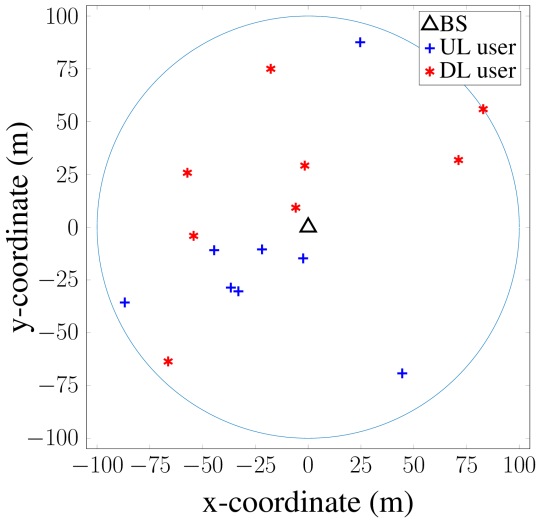
Figure 3: A small cell setup with 8 DL and 8 UL users used in our numerical examples.

Fig. 4 shows the typical convergence behavior of the algorithms for FD schemes, at $\rho^{2}=-30$ dB for convenience. We do not consider the convergence behavior of HD due to the independence of UL and DL SR problems. As can be seen, Algorithm 1 always needs only a few tens of iterations to reach the converging value. The per-iteration optimized value of the proposed algorithm almost saturates from the 30-th iteration, while those of FD-UGFT and FD-CDQS algorithms still increase slightly. In addition, the proposed scheme provides the best performance among the FD-based systems. A method of brute-force search for the integer variables (BFS-IV) based on the proposed algorithm is presented in Fig. 4 as a baseline. In the BFS-IV method, the values of $(\boldsymbol{\Omega},\boldsymbol{\alpha}_{\ell}^{\mathtt{u}},\boldsymbol{\alpha}_{k}^{\mathtt{d}})$ are fixed to each of all possible combinations, and then (16) is used for each case as the proposed FD. In most cases of BFS-IV, $\boldsymbol{\alpha}_{\ell}^{\mathtt{u}}$ and $\boldsymbol{\alpha}_{k}^{\mathtt{d}}$ are fixed to zero, and thus the associated UL transmit power and DL beamforming variables can be set to zero no matter how the other variables are optimized. Therefore, the convergence rate of BFS-IV is faster than those of the three other methods. However, a large number of possible cases for BFS-IV are inapplicable to the FD system. It is further observed that the proposed FD scheme provides the SR close to that of the BFS-IV as Proposition 1 and Lemma 1 hold the optimality.

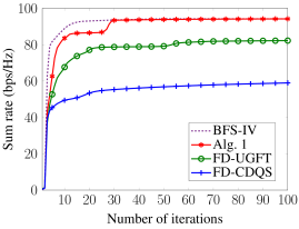
Figure 4: Typical convergence rate of FD schemes with SR maximization problem.

TABLE II: Complexity Comparison

Methods	#Sub-problems	#Variables	#Constraints	Per-iteration complexity
BFS-IV	$s=4^{2}.2^{2K}.2^{2L}$	$v_{1}=4NK+2K+2L+2$	$c_{1}=7K+6L+8$	$s.\mathcal{O}\bigl{(}c_{1}^{2.5}v_{1}^{2}+c_{1}^{3.5}\bigr{)}$
FD-CDQS	1	$v_{2}=N^{2}K+2K+3L$	$c_{2}=6K+7L+1$	$\mathcal{O}\bigl{(}c_{2}^{2.5}v_{2}^{2}+c_{2}^{3.5}\bigr{)}$
FD-UGFT	1	$v_{3}=2NK+12K+14L+4$	$c_{3}=15K+16L+6$	$\mathcal{O}\bigl{(}c_{3}^{2.5}v_{3}^{2}+c_{3}^{3.5}\bigr{)}$
Algorithm 1	8	$v_{1}$	$c_{1}$	$8.\mathcal{O}\bigl{(}c_{1}^{2.5}v_{1}^{2}+c_{1}^{3.5}\bigr{)}$

Besides the convergence speed, an important measure for computation is the per-iteration complexity as it has a significant impact on the total complexity. In each iteration one or more sub-problems are solved, depending on the algorithm structure. As illustrated in Table II, we provide a per-iteration complexity comparison among the algorithms used for FD schemes, in which the complexity of each sub-problem is represented in term of big-O notation as given in [37]. It is true that the number of variables and constraints are the same in BFS-IV and the proposed method, since the power control for BFS-IV is based on Algorithm 1. However, the number of sub-problems for BFS-IV is very high which makes it inapplicable to practical implementation. In the next simulations, we no longer consider BFS-IV due to its extremely high complexity. The number of constraints required by FD-CDQS and the proposed algorithm are comparable. However, since FD-CDQS must handle the rank-1 relaxed variables for the beamforming vectors, the proposed scheme needs much less number of variables, leading to lower per-iteration complexity. As compared to the FD-UGFT method, although Algorithm 1 needs twice the number of the beamforming vector variables, it has a huge payoff related to the number of users. In particular, the largest exponent in big-O notation is with respect to the number of constraints which is significantly reduced in Algorithm 1. Therefore, the proposed method provides a lower complexity, especially when the number of users is large. The per-iteration complexity of the algorithms also has an impact on the required number of iterations to capture a feasible starting point in (31) as investigated in Fig. 5. In Fig. 5, we plot the typical progresses of algorithms to achieve a feasible point from the same initial point which involves the same values of beamforming vector and UL transmit power. Despite starting at the same value, the per-user rate with the proposed algorithm increases to the feasible region (positive per-user rate) more quickly than that with other algorithms. Fig. 5 further depicts the average number of iterations until the feasible point is reached through examining 500 random channels. Algorithm 1 requires the least iterations for the feasible point, as it guarantees less constraints and uses less decision variables. The above results confirm that the proposed method provides a lower complexity in terms of both convergence speed and per-iteration complexity.

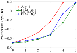
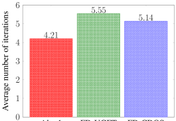
Figure 5: The number of iterations for finding a feasible starting point. (a) A typical iterative progress for finding a feasible point. (b) The average number of iterations to capture a feasible starting point.

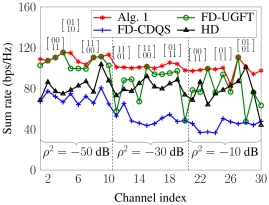
Figure 6: Sum rate versus random channels.

To deeply understand the algorithm, we capture the HA mode selection in two phases under different random channels and residual SI levels. Through the values of $\boldsymbol{\Omega}$, we can perceive the mode changes of HAs so that the system is well adapted to various conditions. In Fig. 6, we randomly generate 30 channels: 10 for every three values of $\rho^{2}\in\{-50,-30,-10\}$ dB. The SRs of the FD-CDQS are worse than those for the other schemes, while the proposed FD provides at least the same performance as the HD or FD-UGFT. If we observe the HA mode selection at the channel index 5, for instance, HA₁ and HA₂ in phase 1 (1-st column of $\boldsymbol{\Omega}$) are set to the Rx (0) and Tx (1) modes, respectively; and vice versa in phase 2 (2-nd column of $\boldsymbol{\Omega}$). Such settings for transmission provide the best performance, as compared to the other FD schemes without Tx/Rx-mode antenna selection. Notably, when $\rho^{2}=-50$ dB, the HA mode selection tends to have FD transmission in both phases. Therefore, the performance of the proposed FD is at least equal to that of FD-UGFT. On the other hand, the trend of the mode selection shifts from the two-phase FD transmission to the hybrid-mode, where both FD and HD are successively used in two phases, and finally to the HD-mode transmission when $\rho^{2}$ becomes large, i.e., $\rho^{2}$ = -10 dB. It demonstrates that the proposed FD is more stable in the change of random channels.

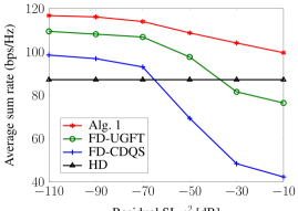
(a) Sum rate versus residual SI.

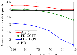
(b) Max-min rate versus residual SI.

Figure 7: The effect of residual SI on the achievable rate.

Fig. 7(a) plots the SR as a function of the residual SI, $\rho^{2}$. Obviously, as the residual SI increases, the performance of three FD schemes deteriorates, while that of the HD system keeps unchanged. As expected, the proposed FD always achieves the highest SR compared to the others. The proposed FD enables the hybrid modes with a dynamically-timed two-phase transmission, and thus, it outperforms the HD scheme even when $\rho^{2}$ becomes more stringent. Otherwise, the advantages of the proposed FD are efficiently exploited by the HA-enabled Tx/Rx-antenna mode. In addition, other FD schemes plummet to under the HD in terms of the SR when the residual SI becomes larger than -40 dB. Fig. 7(b) depicts the max-min rate for both UL and DL users as $\rho^{2}$ increases. As compared to HD, the performance of FD-UGFT is slightly better when $\rho^{2}$ is very small, e.g., $\rho^{2}=\{-110,-90\}$ dB, while FD-CDQS is always inferior to HD in terms of max-min rate because the HD scheme suffers from no SI and CCI, and it has more DoF due to the full-array antennas for transmission. The max-min rate of the proposed FD using a hybrid approach is at least equal to that of HD in case of unfavorable channels for using FD radio.

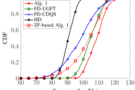
(a) CDF of the sum rate.

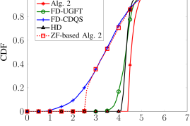
(b) CDF of the max-min rate.

Figure 8: Cumulative distribution functions (CDFs). (a) CDF of the sum rate with $\bar{R}=1$ bps/Hz. (b) CDF of max-min rate.

Fig. 8 shows the CDFs of the SR and max-min rate. We examine 1000 topologies of users’ random positions and 500 random channels for each topology. In both cases, the proposed FD scheme outperforms the others for moderate rate requirements. Interestingly, Fig. 8(a) indicates that the SR optimization is highly flexible for the channel information, including users’ positions and random channels. In fact, the differences between the 5- and 95-percentile of all methods are larger than 20 bps/Hz, which is more than 1 bps/Hz per user on average. Meanwhile, the interval within the same range of percentiles in Fig. 8(b) is lower than 0.5 bps/Hz, except for the FD-CDQS method. This is a result of the SR optimization having the tendency to improve the sum of the channel efficiency as long as the QoS constraints are satisfied, while the max-min optimization improves all users’ rates in association to each other. To examine insight the property of proposed scheme, we provide the CDFs of a baseline method with Alg. 1 using zero-forcing for both UL and DL transmission (ZF-based Alg. 1). As depicted in Fig. 8(a), the ZF-based Alg. 1 method gives the worst performance when compared to the other two-phase FD schemes (FD-UGFT and Alg. 1), which verifies the advantages of MMSE-SIC and beamforming design. Interestingly, the CDF of ZF-based Alg. 2 in Fig. 8(b) reflects both properties of ZF and two-phase transmission. The ZF-based Alg. 2 may utilize the different transmission modes to reduce the SI and CCI, while FD-CDQS still suffers from the interference in the whole time block. Accordingly, though the FD-CDQS method uses MMSE-SIC and beamforming design, ZF-based Alg. 2 with merely canceling the multiuser interference takes more advantage through managing the SI and CCI with two phases. However, Alg. 2 with MMSE-SIC and beamforming design further facilitates the data transmission as compared to ZF-based Alg. 2.

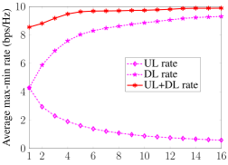
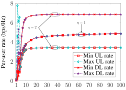
Figure 9: Per-user rate for max-min optimization. (a) Average max-min rate as $\eta=1\rightarrow 16$. (b) Typical convergence behavior.

By using Algorithm 2, Fig. 9(a) shows the per-user rate versus $\eta$. It is clear that the UL users keep the max-min rate, which is the best value of $\phi$ among eight subproblems (34), and the DL users achieve the scaled rate of $\eta\phi$. Although the max-min rate decreases as $\eta$ increases, the total of UL and DL per-user rates increases. This is because when $\eta$ becomes larger, the BS with array antennas effectively favors DL users over UL users. Subsequently, the amount of the increase in the DL rate is more than that of the decrease in the UL rate, which carries the total rate up. To derive further insight into the rates among UL (or DL) users, we investigate the convergences of their maximum and minimum per-user rates, as shown in Fig. 9. For a given value of $\eta$, the maximum and minimum of UL per-user rates converge at the same value. It indicates that the UL per-user rates are equal to each other in the max-min optimization, and similar observation can be made for DL users, as constraints (34c) and (34d) hold. In fact, it first takes several iterations to find a feasible point, and from the 5-th iteration, the maximum and minimum UL (or DL) rates keep almost the same value. It is also true that when $\eta=2$, the UL rates diverge from the DL rates, verifying that the DL gain rates are higher than the UL loss rates.

In Fig. 11, we study the relationship between the SR and max-min rate under different levels of $\eta$ and $\rho^{2}$. As can be observed, the SR is directly proportional to $\eta$ while the max-min rate follows the inverse trend, which is evident from UL rate in Fig. 9(a). The gap of the SR or max-min rate plummets as $\eta$ increases. At $\rho^{2}=-70$ dB, the gap between SRs (or max-min rates) is around 2 bps/Hz (or 1.25 bps/Hz) and less than 1 bps/Hz (or 0.5 bps/Hz) when $\eta$ varies from 1 to 2 and from 8 up to 16, respectively.

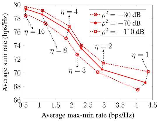
Figure 10: Relationship between sum rate and max-min rate.

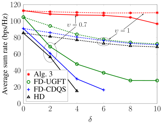
Figure 11: Sum rate with different stochastic error levels.

As the last numerical example, we investigate the effect of different values of channel uncertainties on the SR in Fig. 11. The variances of the CSI errors are modeled as $\epsilon_{\ell}^{\mathtt{u}}=\epsilon_{k}^{\mathtt{d}}=\epsilon_{\ell,k}=\epsilon=\delta r_{sn}^{-\upsilon}$, where $\delta,\upsilon\geq 0$ and $r_{sn}$ is the signal-to-noise ratio [41]. Clearly, the perfect CSI scenario is obtained with $\epsilon=0$ when $\delta=0$ for an arbitrary value of $\upsilon$. To evaluate the performance, we use Algorithm 3 for the proposed robust FD and extend the FD-UGFT [20] and the FD-CDQS [17] with the estimation errors for robust designs. As seen from Fig. 11, the SRs of the existing designs drop quickly as $\delta$ increases. For $\upsilon=0.7$, the existing designs surprisingly deteriorate, and it is even impossible to find a feasible solution at $\delta=4$ (HD) or at $\delta=6$ (FD-CDQS). In contrast, the SR of the proposed FD design is less sensitive to the stochastic error levels, which confirms its robustness against the effect of imperfect CSI as compared to the others.

VII Conclusion

In this paper, we have proposed new joint BS-UE association, time phase and power control designs for the FD MU-MISO systems. The considered problem is either: 1) to maximize the total sum rate subject to the minimum rate requirements for UL and DL users, or 2) to maximize the minimum rate among all users, which is formulated as a mixed-integer non-convex programming. To address the design problem, we have transformed the original problem into subproblems of lower dimensions. Then, iterative low-complexity algorithms have been proposed based on the inner approximation method to solve the sequence of convex programs, exploiting its special properties. Our algorithms with realistic parameters monotonically improve the objective functions and convergence to a stationary point is guaranteed. Through numerical experiments, we have demonstrated the usefulness of our proposed algorithms in improving both the SR and max-min rate, even under strong effects of residual SI. The extension to the case of imperfect CSI has also been considered to further confirm the robustness of the proposed design.

Appendix A Proof of Proposition 1

It is clear that function $f_{\omega}$ in (1) is well-defined since any $\mathbf{z}=[z_{1}\;z_{2}]^{T}\in\{0,1\}^{2\times 1}$ can derive an $f_{\omega}(\mathbf{z})$ in co-domain $\mathcal{B}$. For an arbitrary value of $\hat{z}=\mathrm{b}`b_{1}b_{0}\in\mathcal{B}$, we easily obtain the bit-wise matching as $z_{1}=b_{1}$ and $z_{2}=b_{0}$. For $\mathbf{z}=[z_{1}\;z_{2}]^{T}$, there exists an inverse mapping $\mathbf{z}=f_{\omega}^{-1}(\hat{z})=[b_{1}\;b_{0}]^{T}\in\{0,1\}^{2},\;\forall\hat{z}\in\mathcal{B}$, indicating that $f_{\omega}$ is surjective. Suppose that $f_{\omega}(\mathbf{z}),f_{\omega}(\mathbf{z}^{\prime})\in\mathcal{B}$ and $f_{\omega}(\mathbf{z})=f_{\omega}(\mathbf{z}^{\prime})=\mathrm{b}`b_{1}b_{0}$. According to the definition of $f_{\omega}$ in (1), we get $\mathbf{z}=\mathbf{z}^{\prime}=[b_{1}\;b_{0}]^{T}$, which represents an injection. This verifies the fact that the function $f_{\omega}$ is bijective, and thus a function $g_{\omega}:\;\{0,1\}^{2\times 1}\times\{0,1\}^{2\times 1}\rightarrow\mathcal{B}\times\mathcal{B},\;g_{\omega}(\boldsymbol{\Omega})=[f_{\omega}(\boldsymbol{\omega}_{1})\;f_{\omega}(\boldsymbol{\omega}_{2})]$ is also bijective.

Now, we consider $\boldsymbol{\omega}_{j},\;j=1,2,$ in the objective function of (9). Based on the structure of the formulation problem, $\boldsymbol{\omega}_{j}\;(j=1,2)$ are independently selected in $\{0,1\}^{2\times 1}$ and play the same role as mode selection in two phases. In this manner, $\boldsymbol{\Omega}$ is fixed as a 2-tuple $(\boldsymbol{\omega}_{1},\boldsymbol{\omega}_{2})$, so that we can remove (8b) and (8c) to derive subproblems of lower dimensions.

To reduce the complexity of (9), we further reconstruct the objective function as $f_{R}(\mathbf{X}_{1},\mathbf{X}_{2})=R_{\Sigma}(\mathbf{X}_{1})+R_{\Sigma}(\mathbf{X}_{2})$, where $R_{\Sigma}(\mathbf{X}_{j})\triangleq\sum_{\ell\in\mathcal{L}}\alpha_{\ell,j}^{\mathtt{u}}\bar{\tau}_{j}\ln\bigl{(}1+\gamma_{\ell}^{\mathtt{u}}\bigl{(}\boldsymbol{\omega}_{j},\mathbf{w}_{j},\mathbf{p}_{j}\bigr{)}\bigr{)}+\sum_{k\in\mathcal{K}}\alpha_{k,j}^{\mathtt{d}}\bar{\tau}_{j}\ln\bigl{(}1+\gamma_{k}^{\mathtt{d}}\bigl{(}\boldsymbol{\omega}_{j},\mathbf{w}_{j},\mathbf{p}_{j}\bigr{)}\bigr{)}$ is the sum rate of phase $j$ and $\mathbf{X}_{j}\triangleq\{\boldsymbol{\omega}_{j},\mathbf{w}_{j},\mathbf{p}_{j},\tau,\boldsymbol{\alpha}_{\ell,j}^{\mathtt{u}},\boldsymbol{\alpha}_{k,j}^{\mathtt{d}}\}$, $j=1,2$. It is readily seen that $f_{R}(\mathbf{X}_{1},\mathbf{X}_{2})$ is a symmetric function, meaning $f_{R}(\mathbf{X}_{1}^{*},\mathbf{X}_{2}^{*})=f_{R}(\mathbf{X}_{2}^{*},\mathbf{X}_{1}^{*})$. Moreover, since $g_{\omega}(\boldsymbol{\Omega})$ is a bijection from the finite set $\{0,1\}^{2\times 1}\times\{0,1\}^{2\times 1}$ to the finite set $\mathcal{B}\times\mathcal{B}$, there exists a subset $\mathcal{S}_{\boldsymbol{\Omega}}\subset\{0,1\}^{2\times 1}\times\{0,1\}^{2\times 1}$ and a subset $\mathcal{B}^{\prime}\subset\mathcal{B}\times\mathcal{B}$ such that $g_{\omega}^{-1}(\mathcal{B}^{\prime})=\mathcal{S}_{\boldsymbol{\Omega}}$ and $g_{\omega}(g_{\omega}^{-1}(\mathcal{B}^{\prime}))=\mathcal{B}^{\prime}$. From the symmetry property, we construct a set $\mathcal{B}^{\prime}$ as in (11), which is $\mathcal{B}^{\prime}\subset\mathcal{B}\times\mathcal{B}$, and the search area is thus reduced to a half of $\mathcal{B}\times\mathcal{B}$. For each image $\boldsymbol{\hat{\omega}}\in\mathcal{B}^{\prime}$, the argument $\boldsymbol{\Omega}=g_{\omega}^{-1}(\boldsymbol{\hat{\omega}})\in\mathcal{S}_{\boldsymbol{\Omega}}$ satisfying constraints (8b) and (8c) is used as a constant parameter corresponding to a subproblem, which completes the proof.

Appendix B Bound Tightening in Lemma 1

To examine the effect of $\mathbf{w}_{k,i,j}$ on the optimal value, we consider the beamforming vectors for DL users at the optimum of the subproblem. Let us reconstruct the constraints (8g) and (8h) at the optimum as

$$\sum\nolimits_{k=1}^{K}\bar{\tau}_{j}\|\mathbf{w}_{k,i,j}^{*}\|^{2}+\sum\nolimits_{k=1}^{K}\underset{(i^{\prime},j^{\prime})\neq(i,j)}{\sum\nolimits_{i^{\prime}=1}^{2}\sum\nolimits_{j^{\prime}=1}^{2}}\bar{\tau}_{j}\|\mathbf{w}_{k,i^{\prime},j^{\prime}}^{*}\|^{2}\leq P_{t}^{\text{max}},$$ (48a)

$$\sum\nolimits_{k=1}^{K}\|\mathbf{w}_{k,i,j}^{*}\|^{2}+\sum\nolimits_{k=1}^{K}\|\mathbf{w}_{k,i^{\prime},j}^{*}\|^{2}\leq P_{t}^{\infty},\;i^{\prime}\neq i.$$ (48b)

It is implicit that $\mathbf{w}_{k,i,j}^{*}\in\mathcal{D}_{\mathbf{w}_{k,i,j}}\triangleq\{\mathbf{w}_{k,i,j}\in\mathbb{C}^{N\times 1}|\sum_{k=1}^{K}\bar{\tau}_{j}\|\mathbf{w}_{k,i,j}\|^{2}\in[0,a_{i,j}]\;\&\;\sum_{k=1}^{K}\|\mathbf{w}_{k,i,j}^{*}\|^{2}\in[0,b_{i,j}]\},\forall k\in\mathcal{K}$, where $a_{i,j}\triangleq P_{t}^{\text{max}}-\sum\nolimits_{k=1}^{K}\underset{(i^{\prime},j^{\prime})\neq(i,j)}{\sum\nolimits_{i^{\prime}=1}^{2}\sum\nolimits_{j^{\prime}=1}^{2}}\bar{\tau}_{j}\|\mathbf{w}_{k,i^{\prime},j^{\prime}}^{*}\|^{2}$ and $b_{i,j}\triangleq P_{t}^{\infty}-\sum\nolimits_{k=1}^{K}\|\mathbf{w}_{k,i^{\prime},j}^{*}\|^{2}$. On the other hand, since $\omega_{ij}=0$, the channels corresponding to the $i$-th HA are inactive. According to (5), any value of the beamforming vector $\mathbf{w}_{k,i,j}^{*}\in\mathcal{D}_{\mathbf{w}_{k,i,j}}$ satisfying (48) impacts neither $\gamma_{k}^{\mathtt{d}}\bigl{(}\boldsymbol{\omega}_{j},\mathbf{w}_{j},\mathbf{p}_{j}\bigr{)}$ nor the $k$-th user’s rate. In other words, for $\omega_{ij}=0$, if we change the value of the vector $\mathbf{w}_{k,i,j}^{*}$ at the optimum such that (48) holds, the optimal value would remain unchanged.

Appendix C Uplink SINR

To retrieve the UL information, the optimal weight vector is determined by minimizing the MSE function, i.e.,

$$f^{\text{MSE}}_{\ell,j} =\mathbb{E}\Bigl{[}\bigl{|}x_{\ell,j}^{\mathtt{u}}-\mathbf{u}_{\ell,j}^{H}\mathbf{\hat{y}}_{\ell,j}^{\mathtt{u}}\bigr{|}^{2}\Bigr{]}=1+\mathbf{u}_{\ell,j}^{H}\mathbf{C}_{\mathbf{\hat{y}}_{\ell,j}^{\mathtt{u}}\mathbf{\hat{y}}_{\ell,j}^{\mathtt{u}}}\mathbf{u}_{\ell,j}-2p_{\ell,j}\mathbf{u}_{\ell,j}^{H}\mathbf{\bar{h}}_{\ell,j}^{\mathtt{u}}$$ (49)

where the covariance matrix of $\mathbf{\hat{y}}_{\ell,j}^{\mathtt{u}}$ is calculated by

$$\mathbf{C}_{\mathbf{\hat{y}}_{\ell,j}^{\mathtt{u}}\mathbf{\hat{y}}_{\ell,j}^{\mathtt{u}}} =\mathbb{E}\bigl{[}\mathbf{\hat{y}}_{\ell,j}^{\mathtt{u}}\bigl{(}\mathbf{\hat{y}}_{\ell,j}^{\mathtt{u}}\bigr{)}^{H}\bigr{]}=p_{\ell,j}^{2}\mathbf{\bar{h}}_{\ell,j}^{\mathtt{u}}\bigl{(}\mathbf{\bar{h}}_{\ell,j}^{\mathtt{u}}\bigr{)}^{H}+\boldsymbol{\hat{\Psi}}_{\ell,j}$$ (50)

with $\boldsymbol{\hat{\Psi}}_{\ell,j}\triangleq\sum_{\ell^{\prime}=\ell+1}^{L}p_{\ell^{\prime},j}^{2}\mathbf{\bar{h}}_{\ell^{\prime},j}^{\mathtt{u}}\bigl{(}\mathbf{\bar{h}}_{\ell^{\prime},j}^{\mathtt{u}}\bigr{)}^{H}+\sum_{\ell^{\prime}=1}^{L}p_{\ell^{\prime},j}^{2}\epsilon_{\ell^{\prime}}^{\mathtt{u}}\boldsymbol{\bar{\Lambda}}_{j}+\rho^{2}\sum_{k=1}^{K}\mathbf{\tilde{G}}_{j}^{H}\mathbf{w}_{k,j}\mathbf{w}_{k,j}^{H}\mathbf{\tilde{G}}_{j}+\sigma_{\mathtt{U}}^{2}\mathbf{I}$ and $\mathbf{\bar{h}}_{\ell,j}^{\mathtt{u}}\triangleq\boldsymbol{\bar{\Lambda}}_{j}\mathbf{\hat{h}}_{\ell}^{\mathtt{u}}$. The optimal solution for MSE minimization satisfying $\nabla_{\mathbf{u}_{\ell,j}^{H}}f^{\text{MSE}}_{\ell,j}=0$ is

$$\mathbf{u}_{\ell,j}=p_{\ell,j}\mathbf{C}_{\hat{\mathbf{y}}_{\ell,j}^{\mathtt{u}}\hat{\mathbf{y}}_{\ell,j}^{\mathtt{u}}}^{-1}\mathbf{\bar{h}}_{\ell,j}^{\mathtt{u}}$$ (51)

showing (37).

Furthermore, the information detection is performed as $\hat{x}_{\ell,j}^{\mathtt{u}}=\mathbf{u}_{\ell,j}^{H}\mathbf{\hat{y}}_{\ell,j}^{\mathtt{u}}=s_{\ell,j}+z_{\ell,j},$ where the expected signal and interference-plus-noise are respectively given by

$$s_{\ell,j} =\mathbf{u}_{\ell,j}^{H}\mathbf{\bar{h}}_{\ell,j}^{\mathtt{u}}x_{\ell,j}^{\mathtt{u}}=p_{\ell,j}^{2}\bigl{(}\mathbf{\bar{h}}_{\ell,j}^{\mathtt{u}}\bigr{)}^{H}\mathbf{C}_{\mathbf{\hat{y}}_{\ell,j}^{\mathtt{u}}\mathbf{\hat{y}}_{\ell,j}^{\mathtt{u}}}^{-1}\mathbf{\bar{h}}_{\ell,j}^{\mathtt{u}}x_{\ell,j}^{\mathtt{u}},$$ (52)

$$z_{\ell,j} =\mathbf{u}_{\ell,j}^{H}\bigl{(}\sum\nolimits_{\ell^{\prime}>\ell}^{L}p_{\ell^{\prime},j}\mathbf{\bar{h}}_{\ell^{\prime}}^{\mathtt{u}}x_{\ell^{\prime},j}^{\mathtt{u}}+\sum\nolimits_{\ell^{\prime}=1}^{L}p_{\ell^{\prime},j}\boldsymbol{\bar{\Lambda}}_{j}\boldsymbol{\Delta}\mathbf{h}_{\ell^{\prime}}^{\mathtt{u}}x_{\ell^{\prime},j}^{\mathtt{u}}+\rho\sum\nolimits_{k=1}^{K}\mathbf{\tilde{G}}_{j}^{H}\mathbf{w}_{k,j}x_{k,j}^{\mathtt{d}}+\mathbf{n}_{\ell,j}\bigr{)}.$$ (53)

From (51)-(53), the SINR of $\mathtt{U}_{\ell}^{\mathtt{u}}$ in phase $j$ by treating the CSI errors as noise is derived as

$$\hat{\gamma}_{\ell}^{\mathtt{u}}(\boldsymbol{\omega}_{j},\mathbf{w}_{j},\mathbf{p}_{j})=\frac{\mathbb{E}\bigl{[}s_{\ell,j}s_{\ell,j}^{H}\bigr{]}}{\mathbb{E}\bigl{[}z_{\ell,j}z_{\ell,j}^{H}\bigr{]}} =\frac{p_{\ell,j}^{2}\bigl{(}\mathbf{\bar{h}}_{\ell,j}^{\mathtt{u}}\bigr{)}^{H}\mathbf{C}_{\mathbf{\hat{y}}_{\ell,j}^{\mathtt{u}}\mathbf{\hat{y}}_{\ell,j}^{\mathtt{u}}}^{-1}\mathbf{\bar{h}}_{\ell,j}^{\mathtt{u}}}{1-p_{\ell,j}^{2}\bigl{(}\mathbf{\bar{h}}_{\ell,j}^{\mathtt{u}}\bigr{)}^{H}\mathbf{C}_{\mathbf{\hat{y}}_{\ell,j}^{\mathtt{u}}\mathbf{\hat{y}}_{\ell,j}^{\mathtt{u}}}^{-1}\mathbf{\bar{h}}_{\ell,j}^{\mathtt{u}}}.$$ (54)

By applying the matrix inversion lemma to the denominator of (54), i.e., $1-p_{\ell,j}^{2}\bigl{(}\mathbf{\bar{h}}_{\ell,j}^{\mathtt{u}}\bigr{)}^{H}\mathbf{C}_{\mathbf{\hat{y}}_{\ell,j}^{\mathtt{u}}\mathbf{\hat{y}}_{\ell,j}^{\mathtt{u}}}^{-1}\mathbf{\bar{h}}_{\ell,j}^{\mathtt{u}}=\bigl{(}1+p_{\ell,j}^{2}(\mathbf{\bar{h}}_{\ell,j}^{\mathtt{u}})^{H}\boldsymbol{\hat{\Psi}}_{\ell,j}^{-1}\mathbf{\bar{h}}_{\ell,j}^{\mathtt{u}}\bigr{)}^{-1}$, (54) can be further simplified as

$$\hat{\gamma}_{\ell}^{\mathtt{u}}(\boldsymbol{\omega}_{j},\mathbf{w}_{j},\mathbf{p}_{j}) =\frac{1-\bigl{(}1+p_{\ell,j}^{2}(\mathbf{\bar{h}}_{\ell,j}^{\mathtt{u}})^{H}\boldsymbol{\hat{\Psi}}_{\ell,j}^{-1}\mathbf{\bar{h}}_{\ell,j}^{\mathtt{u}}\bigr{)}^{-1}}{\bigl{(}1+p_{\ell,j}^{2}(\mathbf{\bar{h}}_{\ell,j}^{\mathtt{u}})^{H}\boldsymbol{\hat{\Psi}}_{\ell,j}^{-1}\mathbf{\bar{h}}_{\ell,j}^{\mathtt{u}}\bigr{)}^{-1}}=p_{\ell,j}^{2}\bigl{(}\mathbf{\bar{h}}_{\ell,j}^{\mathtt{u}}\bigr{)}^{H}\boldsymbol{\hat{\Psi}}_{\ell,j}^{-1}\mathbf{\bar{h}}_{\ell,j}^{\mathtt{u}}$$ (55)

showing (38), and the proof is completed.

References

- [1] H. V. Nguyen, V.-D. Nguyen, O. A. Dobre, and O.-S. Shin, “Sum rate maximization based on sub-array antenna selection in a full-duplex system,” in Proc. IEEE Global Commun. Conf. (GLOBECOM), Dec. 2017, pp. 1–6.
- [2] J. Mietzner, R. Schober, L. Lampe, W. H. Gerstacker, and P. A. Hoeher, “Multiple-antenna techniques for wireless communications: A comprehensive literature survey,” IEEE Commun. Surveys Tutorials, vol. 11, no. 2, pp. 87–105, 2nd Quarter 2009.
- [3] A. Sabharwal, P. Schniter, D. Guo, D. W. Bliss, S. Rangarajan, and R. Wichman, “In-band full-duplex wireless: Challenges and opportunities,” IEEE J. Sel. Areas Commun., vol. 32, no. 9, pp. 1637–1652, Feb. 2014.
- [4] Z. Zhang, X. Chai, K. Long, A. V. Vasilakos, and L. Hanzo, “Full duplex techniques for 5G networks: Self-interference cancellation, protocol design, and relay selection,” IEEE Commun. Mag., vol. 53, no. 5, pp. 128–137, May 2015.
- [5] V. W. Wong, R. Schober, D. W. K. Ng, and L.-C. Wang, Key Technologies for 5G Wireless Systems. Cambridge, MA, USA: Cambridge Univ. Press, 2017.
- [6] A. Yadav, G. I. Tsiropoulos, and O. A. Dobre, “Full duplex communications: Performance in ultra-dense small-cell wireless networks,” IEEE Veh. Technol. Mag., Apr. 2018. [Online]. Available: https://arxiv.org/ftp/arxiv/papers/1803/1803.00473.pdf
- [7] M. Duarte, C. Dick, and A. Sabharwal, “Experiment-driven characterization of full-duplex wireless systems,” IEEE Trans. Wireless Commun., vol. 11, no. 12, pp. 4296–4307, Dec. 2012.
- [8] D. Bharadia, E. McMilin, and S. Katti, “Full duplex radios,” in Proc. ACM SIGCOMM Computer Commun. Review, vol. 43, no. 4, 2013, pp. 375–386.
- [9] D. Korpi, J. Tamminen, M. Turunen, T. Huusari, Y. S. Choi, L. Anttila, S. Talwar, and M. Valkama, “Full-duplex mobile device: Pushing the limits,” IEEE Commun. Mag., vol. 54, no. 9, pp. 80–87, Sept. 2016.
- [10] L. Laughlin, M. A. Beach, K. A. Morris, and J. L. Haine, “Electrical balance duplexing for small form factor realization of in-band full duplex,” IEEE Commun. Mag., vol. 53, no. 5, pp. 102–110, May 2015.
- [11] A. Yadav, O. A. Dobre, and H. V. Poor, “Is self-interference in full-duplex communications a foe or a friend?,” IEEE Signal Process. Lett., Feb. 2018, DOI:10.1109/LSP.2018.2802780.
- [12] B. P. Day, A. R. Margetts, D. W. Bliss, and P. Schniter, “Full-duplex bidirectional MIMO: Achievable rates under limited dynamic range,” IEEE Trans. Signal Process., vol. 60, no. 7, pp. 3702–3713, July 2012.
- [13] N. Zlatanov, E. Sippel, V. Jamali, and R. Schober, “Capacity of the Gaussian two-hop full-duplex relay channel with residual self-interference,” IEEE Trans. Commun., vol. 65, no. 3, pp. 1005–1021, Mar. 2017.
- [14] D. Nguyen, L.-N. Tran, P. Pirinen, and M. Latva-aho, “Precoding for full duplex multiuser MIMO systems: Spectral and energy efficiency maximization,” IEEE Trans. Signal Process., vol. 61, no. 16, pp. 4038–4050, Aug. 2013.
- [15] V.-D. Nguyen, T. Q. Duong, H. D. Tuan, O.-S. Shin, and H. V. Poor, “Spectral and energy efficiencies in full-duplex wireless information and power transfer,” IEEE Trans. Commun., vol. 65, no. 5, pp. 2220–2233, May 2017.
- [16] A. Yadav, O. A. Dobre, and N. Ansari, “Energy and traffic aware full duplex communications for 5G systems,” IEEE Access, vol. 5, pp. 11 278–11 290, May 2017.
- [17] D. Nguyen, L.-N. Tran, P. Pirinen, and M. Latva-aho, “On the spectral efficiency of full-duplex small cell wireless systems,” IEEE Trans. Wireless Commun., vol. 13, no. 9, pp. 4896–4910, Sept. 2014.
- [18] H. H. M. Tam, H. D. Tuan, and D. T. Ngo, “Successive convex quadratic programming for quality-of-service management in full-duplex MU-MIMO multicell networks,” IEEE Trans. Commun., vol. 64, no. 6, pp. 2340–2353, Jun. 2016.
- [19] P. Aquilina, A. C. Cirik, and T. Ratnarajah, “Weighted sum rate maximization in full-duplex multi-user multi-cell MIMO networks,” IEEE Trans. Commun., vol. 65, no. 4, pp. 1590–1608, Apr. 2017.
- [20] V.-D. Nguyen, H. V. Nguyen, C. T. Nguyen, and O.-S. Shin, “Spectral efficiency of full-duplex multiuser system: Beamforming design, user grouping, and time allocation,” IEEE Access, vol. 5, pp. 5785–5797, Mar. 2017.
- [21] A. C. Cirik, S. Biswas, S. Vuppala, and T. Ratnarajah, “Robust transceiver design for full duplex multiuser MIMO systems,” IEEE Wireless Commun. Lett., vol. 5, no. 3, pp. 260–263, June 2016.
- [22] A. C. Cirik, M. J. Rahman, and L. Lampe, “Robust fairness transceiver design for a full-duplex MIMO multi-cell system,” IEEE Trans. Commun., vol. 66, no. 3, pp. 1027–1041, March 2018.
- [23] V.-D. Nguyen, H. V. Nguyen, O. A. Dobre, and O.-S. Shin, “A new design paradigm for secure full-duplex multiuser systems,” IEEE J. Select. Areas Commun., 2018. [Online]. Available: https://arxiv.org/abs/1801.00963
- [24] C. Nam, C. Joo, and S. Bahk, “Joint subcarrier assignment and power allocation in full-duplex OFDMA networks,” IEEE Trans. Wireless Commun., vol. 14, no. 6, pp. 3108–3119, Jun. 2015.
- [25] B. Di, S. Bayat, L. Song, Y. Li, and Z. Han, “Joint user pairing, subchannel, and power allocation in full-duplex multi-user OFDMA networks,” IEEE Trans. Wireless Commun., vol. 15, no. 12, pp. 8260–8272, Dec. 2016.
- [26] J. M. B. da Silva, G. Fodor, and C. Fischione, “Fast-Lipschitz power control and user-frequency assignment in full-duplex cellular networks,” IEEE Trans. Wireless Commun., vol. 16, no. 10, pp. 6672–6687, Oct. 2017.
- [27] M. Ahn, H. Kong, H. M. Shin, and I. Lee, “A low complexity user selection algorithm for full-duplex MU-MISO systems,” IEEE Trans. Wireless Commun., vol. 15, no. 11, pp. 7899–7907, Nov. 2016.
- [28] K. Yang, H. Cui, L. Song, and Y. Li, “Efficient full-duplex relaying with joint antenna-relay selection and self-interference suppression,” IEEE Trans. Wireless Commun., vol. 14, no. 7, pp. 3991–4005, July 2015.
- [29] S. Jang, M. Ahn, H. Lee, and I. Lee, “Antenna selection schemes in bidirectional full-duplex MIMO systems,” IEEE Trans. Veh. Technol., vol. 65, no. 12, pp. 10097–10100, Dec. 2016.
- [30] T. Riihonen, S. Werner, and R. Wichman, “Mitigation of loopback self-interference in full-duplex MIMO relays,” IEEE Trans. Signal Process., vol. 59, no. 12, pp. 5983–5993, Dec. 2011.
- [31] D. Tse and P. Viswanath, Fundamentals of Wireless Communication. Cambridge Univ. Press, UK, 2005.
- [32] M. Tawarmalani and N. V. Sahinidis, Convexification and Global Optimization in Continuous and Mixed-Integer Nonlinear Programming: Theory, Algorithms, Software, and Applications. Norwell, MA, USA: Kluwer Academic Publishers, 2002.
- [33] B. R. Marks and G. P. Wright, “A general inner approximation algorithm for nonconvex mathematical programs,” Operations Research, vol. 26, no. 4, pp. 681–683, Jul.-Aug. 1978.
- [34] H. Tuy, Convex Analysis and Global Optimization. Kluwer Academic, 2001.
- [35] S. Boyd and L. Vandenberghe, Convex Optimization. Cambridge University Press, 2004.
- [36] “I. MOSEK aps,” 2014. [Online]. Available: at http://www.mosek.com
- [37] D. Peaucelle, D. Henrion, Y. Labit, and K. Taitz, “User’s guide for SeDuMi interface 1.04,” in LAAS-CNRS, Toulouse, France, Jun. 2002.
- [38] J. R. Munkres, Topology: A First Course. Englewood Cliffs, NJ: Prentice-Hall, 1974.
- [39] K. Bestuzheva and H. Hijazi, “Invex optimization revisited,” July 2017. [Online]. Available: https://arxiv.org/abs/1707.01554v1
- [40] 3GPP Technical Specification Group Radio Access Network, Evolved Universal Terrestrial Radio Access (E-UTRA): Further Advancements for E-UTRA Physical Layer Aspects (Release 9), document 3GPP TS 36.814 V9.0.0, 2010.
- [41] J. Maurer, J. Jalden, D. Seethaler, and G. Matz, “Vector perturbation precoding revisited,” IEEE Trans. Signal Process., vol. 59, no. 1, pp. 315–328, Jan. 2011.