Ergodicity of some dynamics of DNA sequences

Abstract

We define interacting particle systems on configurations of the integer lattice (with values in some finite alphabet) by the superimposition of two dynamics: a substitution process with finite range rates, and a circular permutation mechanism (called “cut-and-paste”) with possibly unbounded range. The model is motivated by the dynamics of DNA sequences: we consider an ergodic model for substitutions, the RN+YpR model ([BGP08]), with three particular cases, the models JC+$\mathtt{c}$p$\mathtt{g}$, T92+$\mathtt{c}$p$\mathtt{g}$, and RNc+YpR. We investigate whether they remain ergodic with the additional cut-and-paste mechanism, which models insertions and deletions of nucleotides. Using either duality or attractiveness techniques, we provide various sets of sufficient conditions, concerning only the substitution rates, for ergodicity of the superimposed process. They imply ergodicity of the models JC+$\mathtt{c}$p$\mathtt{g}$, T92+$\mathtt{c}$p$\mathtt{g}$ as well as the attractive RNc+YpR, all with an additional cut-and-paste mechanism.

To Guy Fayolle, on the occasion of his birthday

1 Introduction

Motivated by biological models for the evolution of DNA sequences, this paper contributes to the classical topic of ergodicity of interacting particle systems (see e.g. [Lig05]). Let us first give the biological context, then explain the interacting particle system it induces, and how we tackle its ergodicity. This last point corresponds to the intriguing question of the ergodicity for a superimposition of an ergodic particle system (here a generalized spin system) and of a non ergodic one (here cyclic permutations which generalize exclusion processes). The spin values belong to a finite alphabet of size larger than two, which adds a difficulty.

The biological set-up. The study of evolutionary relationships among living organisms has entered the genomic age in the past decades. To model the evolution of DNA sequences remains an important and difficult part of phylogenetic analysis. Generally, every method of phylogenetic reconstruction at the molecular level is based on a probabilistic model, for codons or for nucleotides. Jukes & Cantor, in [JC69], were the first to introduce a probabilistic model, the (JC) model, to study the changes in DNA sequences. In the (JC) model, DNA sequences are encoded as elements of $\mathscr{A}^{N}$, where the positive integer $N$ stands for the number of nucleotides in one strand of the DNA molecule, and $\mathscr{A}$ for the nucleotide alphabet $\{\mathtt{a},\mathtt{t},\mathtt{c},\mathtt{g}\}$, where the letters represent adenine, thymine, cytosine and guanine respectively. The (JC) model deals with the product of $N$ independent identically distributed continuous-time Markov chains modelling single site nucleotide substitutions.

The substitution-rate matrix in the (JC) model is the simplest possible because all substitutions occur at the same rate. Since then, other nucleotide substitution processes have been introduced to refine this matrix (see for instance [Kim80, Fel81, HKY85, Tam92, TN93, Yan94]) until the generalized time reversible (GTR) model introduced in [Tav86] which is such that the Markov process is reversible, and with no more restriction on the structure of the matrix. In all these processes, the independence assumption on sites was kept. As a consequence, there exists a unique stationary probability measure for the process, which is product. This means for instance that in a long DNA sequence at equilibrium the frequency of a dinucleotide $x$p$y$ should be the product of the $x$ and $y$ frequencies (where, for subsets $X$ and $Z$ of $\mathscr{A}$, $X$p$Z$ is the collection of dinucleotides in $X\times Z$, and we write $x$p$y$ instead of $\{x\}$p$\{y\}$).

But this is actually not the case in some biological contexts. Indeed, since the studies of [JKK61] and [STK62], it is well known that the dinucleotide $\mathtt{c}$p$\mathtt{g}$ is less frequently present in many mammals DNA than it would be expected from base composition. Support for the $\mathtt{c}$p$\mathtt{g}$ deficiency to be related to DNA methylation was provided in [Bir80]: the substitution rate of cytosine by thymine is higher in methylated $\mathtt{c}$p$\mathtt{g}$ than in other dinucleotides. Therefore, more realistic substitution models incorporating such neighboring effects have been introduced by [DG00] with their Tamura+$\mathtt{c}$p$\mathtt{g}$ model. To evade the dependency between neighbors, in [DG00] there is an approximation for frequencies of trinucleotides to capture some features of the true model. Bérard et al. in [BGP08] extended the latter model to the RN+YpR model and assessed rigorously the effect of neighbor-dependent substitutions. There, DNA sequences are encoded as (doubly infinite) elements of $\mathscr{A}^{\mathbb{Z}}$ and their dynamics are studied through the techniques of interacting particle systems. The properties of the RN+YpR model have been used to infer phylogenetic distances in [Fal10] or $\mathtt{c}$p$\mathtt{g}$ hypermutability rates in [BG12].

But substitutions are not the only way to alter DNA sequences. For example, one may add several extra nucleotides to a DNA sequence by insertions, or remove them by deletions. In the model of [TKF91], single sites are inserted or deleted with rates independent of their positions, and this is superimposed to independent substitutions. There, DNA sequences have a variable (but finite) length along time and are encoded as elements of $\bigcup_{N}\mathscr{A}^{N}$. We would like to do for neighbor-dependent substitution processes on DNA sequences what was done in [TKF91] for independent substitutions. The DNA sequences are viewed, as above, as elements of $\mathscr{A}^{\mathbb{Z}}$. To avoid mathematical difficulties due to the insertion-deletion mechanisms (an insertion of a single nucleotide induces a shift of the whole sequence and leads to infinite range interactions), we require that an insertion and a deletion occur at the same time. To that purpose, we introduce a mechanism that we call “cut-and-paste”, whose name is inspired from the classification proposed by [Fin89] for transposable elements. The latter, discovered by [McC53], are a type of DNA that can move around within the genome and can be distinguished in two classes : class I is commonly called “copy-and-paste”, and class II, “cut-and-paste”. In our settings, we consider the simplest cut-and-paste mechanism, that is, the transfer of one nucleotide into the sequence as shown on Figure 1. There, the transfer of nucleotide $\mathtt{t}$ can be seen as its deletion and reinsertion three nucleotides further.

Figure 1: One example of the cut-and-paste of a nucleotide into the sequence

The modelling by a particle system, and the question of its ergodicity. We consider configurations that can take values in some finite alphabet on each site of the integer lattice, as detailed above; thus the alphabet will consist of the nucleotides $\mathtt{a},\mathtt{c},\mathtt{g}$ and $\mathtt{t}$, but the questions we ask are not relying on this specific choice. On this configuration space, we superimpose two dynamics. The first one is given by a substitution process, and the second one by a cut-and-paste mechanism with a rate $\rho>0$. The substitution process is quite general and includes for instance the stochastic Ising model with finite rate of dependence. The cut-and-paste process can have unbounded range and permutes the values of a certain interval of sites; it can be seen as a generalization of an exclusion process.

In this superimposition, the first dynamics is ergodic but not the second one. Note that ergodicity of our process, at least in the case of finite range permutations, would follow from the “Positive Rates Conjecture” which says that in dimension $1$, a finite range interacting particle system with strictly positive transition rates is ergodic, see [Lig05], page 201. The status of this conjecture is not clear to us, see [Gra01]. It has been proved for attractive nearest-neighbor spin systems (a spin system is an interacting particle system with two states such that only one coordinate can change in each transition, see [Lig05], Chapter II) in [Gra82]. But, even if the permutations have finite range, our model does not fit into this frame, since the cut-and-paste mechanism changes several sites at the same time, and moreover we work with an alphabet of more than two values. There is a general sufficient condition for ergodicity, the so-called Dobrushin’s “$M<\varepsilon$” condition (see [Dob71], or [Lig05], Chapter I). However, this condition is far from being necessary: For instance, it gives ergodicity of the one-dimensional nearest-neighbor stochastic Ising model only for high values of the temperature. Note that if a process does fit the “$M<\varepsilon$” condition, adding a small amount of “stirring” will not alter the validity of the latter, hence the superimposition with a stirring mechanism (which permutes the values on two neighboring sites) is ergodic for $\rho$ small enough.

To derive ergodicity conditions for our superimposition of two dynamics, we use two powerful techniques: the first one is based on duality, and the second one on attractiveness and couplings. Our results involve only the parameters of the substitution process, thus they are valid for any value of $\rho$. First we use duality through a generalization of a coupling technique with branching processes due to [Fer90] to show that, in a certain range of parameters of the substitution process, the superimposition is ergodic. We then apply this general result to our generic example, the RN+YpR substitution model with an additional cut-and-paste mechanism. Second, in the spirit of [GS10, Bor11], we derive sufficient conditions on the substitution rates for attractiveness of the superimposition; assuming them, we obtain by different approaches sufficient conditions on theses rates for ergodicity. While our first results are general, the following ones concern the RN+YpR model with cut-and-paste mechanism. They imply that its particular cases, the models JC+$\mathtt{c}$p$\mathtt{g}$, T92+$\mathtt{c}$p$\mathtt{g}$, as well as the RNc+YpR model in case it is attractive, are ergodic when they are superimposed with a cut-and-paste mechanism.

The paper is organized as follows. In Section 2 we define the model and the examples, for which we state ergodicity results (Theorems 2.3 and 2.5). In Section 3, we give the set-up for generalized duality, then state general ergodicity results (Theorems 3.1 and 3.4), proved in Section 5; we then prove Theorem 2.3. In Section 4, we give the set-up for attractiveness, then state various results (some general, some for our examples) for ergodicity, proved in Section 6, and we prove Theorem 2.5.

2 Definitions and examples

In Section 2.1, we introduce our set-up: two types of interacting particle systems on $X=\mathscr{A}^{\mathbb{Z}}$, namely a substitution and a cut-and-paste processes, that we superimpose. We then define in Section 2.2 the examples that will illustrate our analysis along the paper. In Section 2.3, we state for them the ergodicity results that follow from our analysis of the superimposed process, done in the rest of the paper.

2.1 The particle system

For an analytic study of the construction and basic properties of these systems, we refer to the seminal book [Lig05], on which we rely for sufficient existence conditions of our dynamics. We will give in Section 5 a graphical construction of the latter, which will be the first step to prove ergodicity results through duality.

2.1.1 Substitution process

In such a process, only one coordinate changes in each transition. The transition mechanism is specified by a non-negative function $c(\cdot)$ defined on ${\mathbb{Z}}\times\mathscr{A}\times X$. For $\eta\in X$, $x\in{\mathbb{Z}}$ and $a\in\mathscr{A}$, $c(x,a,\eta)$ represents the rate at which the coordinate $\eta(x)$ flips to $a$ when the system is in state $\eta$, that is the rate at which $\eta$ changes to $\eta^{x}_{a}$ defined by

$$\eta^{x}_{a}(z)=\left\{\begin{array}[]{lll}\eta(z)&\mbox{if}&z\neq x,\\ a&\mbox{if}&z=x.\end{array}\right.$$

We assume that the rates $c(x,a,\cdot)$ are translation invariant, i.e. $c(x,a,\eta)=c(0,a,\tau_{x}\eta)$ where $\tau_{x}$ denotes the shift by $x$ on $X$ (given by $\tau_{x}\eta(y)=\eta(x+y)$, for all $y\in{\mathbb{Z}}$). From now on, we write $c(a,\eta)$ for $c(0,a,\eta)$. We further assume that, for any target $a$, the function $c(a,\cdot)$ depends on $\eta\in X$ only through a finite set $S(a)\subset{\mathbb{Z}}$ depending on $a$.

The pregenerator $\mathscr{L}_{1}$ of the substitution process is defined on a cylinder function $f$ on $X$ (that is, a function depending on a finite number of coordinates) by

$$\mathscr{L}_{1}f(\eta)=\sum_{x\in{\mathbb{Z}}}\sum_{a\in\mathscr{A}}\ c(a,\tau_{x}\eta)\big{[}f(\eta^{x}_{a})-f(\eta)\big{]}.$$ (2.1)

Let

$$m =\inf\{c(a,\eta)\,:\,a\in\mathscr{A},\eta\in X\},$$ (2.2)

$$K =\sup\{c(a,\eta)\,:\,a\in\mathscr{A},\eta\in X\},$$ (2.3)

$$s =\sup\{|S(a)|\,:\,a\in\mathscr{A}\},$$ (2.4)

where $|S|$ denotes the cardinality of the set $S$. Because the alphabet $\mathscr{A}$ is finite, we have that

$$s<+\infty,\quad K<+\infty.$$ (2.5)

This is a sufficient condition for the existence of a Markov process with pregenerator $\mathscr{L}_{1}$ (see Theorem I.3.9 in [Lig05]). For Theorem 3.1 and for our examples, we will assume

$$m>0,$$ (2.6)

which is a standard assumption for ergodicity results (see e.g. [Gra01], [Gra82]).

2.1.2 Cut-and-paste process

In this process, not only one coordinate changes in each transition (as it can be seen on Figure 1 where the transfer of nucleotide $\mathtt{t}$ induces a change of four coordinates because of the shift to the left for the segment $\mathtt{c}\mathtt{g}\mathtt{c}$). The transition mechanisms are circular permutations $\sigma_{x,y}$ (for $x\not=y\in{\mathbb{Z}}$) of finitely many sites of ${\mathbb{Z}}$ and are specified by a transition probability matrix $p$ on ${\mathbb{Z}}\times{\mathbb{Z}}$.
For $\eta\in X$ and a pair of sites $x\neq y$, let $\sigma_{x,y}(\eta)$ be the configuration defined by

$$\sigma_{x,y}(\eta)(z)=\eta\big{[}\sigma_{x,y}^{-1}(z)\big{]},\quad\forall z\in{\mathbb{Z}},$$

where $\sigma_{x,y}$ is defined for any $x<y$ as

$$\sigma_{x,y}(z)=\left\{\begin{array}[]{lll}z&\mbox{if}&z\notin\{x,x+1,\dots,y\},\\ y&\mbox{if}&z=x,\\ z-1&\mbox{if}&x<z\leqslant y,\end{array}\right.$$

and for any $x>y$ as

$$\sigma_{x,y}(z)=\left\{\begin{array}[]{lll}z&\mbox{if}&z\notin\{y,y+1,\dots,x\},\\ y&\mbox{if}&z=x,\\ z+1&\mbox{if}&y\leqslant z<x.\end{array}\right.$$

The case $x<y$ corresponds to a shift to the left of the coordinates from site $x+1$ to site $y$ as it can be seen on the top of Figure 2, whereas $x>y$ corresponds to a shift to the right of the coordinates from $y$ to $x-1$ as it can be seen on the bottom of Figure 2.

Figure 2: Transfer of the coordinate $\eta(x)$ from site $x$ to site $y$ when $x<y$ (top panel) or when $x>y$ (bottom panel)

The rate at which $\eta$ changes to $\sigma_{x,y}(\eta)$ is $p(x,y)$. We assume that $p$ is translation invariant on ${\mathbb{Z}}$, that is, $p(x,y)=p(0,y-x)$ for all $x,y\in{\mathbb{Z}}$. We do not assume that $p$ is symmetric, hence the “rate of transfer” $p(x,y)$ at which the coordinate $\eta(x)$ is transferred to site $y$ might depend not only on the distance $|y-x|$ but also on the direction of the transfer.
The pregenerator $\mathscr{L}_{2}$ of a cut-and-paste process is defined on a cylinder function $f$ on $X$ by

$$\mathscr{L}_{2}f(\eta)=\sum_{x,y\in{\mathbb{Z}}}p(x,y)\big{[}f(\sigma_{x,y}(\eta))-f(\eta)\big{]}.$$ (2.7)

A sufficient condition for the existence of the cut-and-paste process, that we assume from now on, is (see [Lig05], [AFS04])

$$\sum|x|p(0,x)<\infty.$$ (2.8)

Remark 2.1.

(i) We mentioned that $p$ is not necessarily symmetric because [Kov05] studies invariant measures of particle systems that interact via finite range permutations, which is a more general system than a cut-and-paste process, but with the restriction that the permutation $\sigma$ has the same rate of occurrence than $\sigma^{-1}$, which is equivalent in our case to the symmetry of $p$.
Ergodicity of cellular automata that are superimpositions of Glauber dynamics and permutations is studied in [Fer91].
(ii) For simplicity, we stick here to circular permutations. As it will become clear from the proofs, we could also consider more general permutations of $\eta(x),\eta(x+1),\ldots,\eta(y)$ or $\eta(y),\eta(y+1),\ldots\eta(x)$, respectively, resulting in different biological interpretations than the one we gave in the introduction.
(iii) The cut-and-paste process generalizes a stirring process, which is such that $p(.,.)$ is symmetric and nearest-neighbor, so that only two coordinates change in a transition.

2.1.3 The superimposition

Fix a constant $\rho>0$ and define the pregenerator $\mathscr{L}$ on a cylinder function $f$ on $X$ as

$$\mathscr{L}f=\mathscr{L}_{1}f+\rho\mathscr{L}_{2}f.$$ (2.9)

We are interested in the ergodic properties of the interacting particle system with pregenerator $\mathscr{L}$, that is, the superimposition of a substitution and a cut-and-paste process. This superimposition is well defined by assumptions (2.5) and (2.8). We denote by $\mathscr{P}(X)$ the set of probability measures on $X$, by $\SS$ the set of translation invariant probability measures on $X$. For the superimposition we denote by $\mathscr{I}$ the set of invariant probability measures.

Recall that (Definition I.1.9 in [Lig05]) ergodicity of a Markov process with values in $X=\mathscr{A}^{\mathbb{Z}}$ means that there is exactly one invariant probability measure, denoted e.g. by $\mu$, and for each starting point, the law of the process converges to this invariant probability measure.

This ergodic process is moreover exponentially ergodic ([Fer90], page 1526) if for any bounded cylinder function $f$ on $X$, there exist positive constants $a_{1}=a_{1}(f),a_{2}$ such that for any initial probability measure $\nu$, for any $t\geqslant 0$, we have

$$\left|\int fd(\nu S(t))-\int fd\mu\right|<a_{1}\mathrm{e}^{-a_{2}t}.$$ (2.10)

The simplest ergodic substitution processes are the independent ones. As expected, the superimposition of a cut-and-paste mechanism does not affect the ergodic properties and the invariant probability measure of such processes. In this case, we do not need assumption (2.6), and moreover $s=1$ (see (2.4)).

Lemma 2.2.

Assume that the rate function $c(\cdot)$ can be written as

$$c(x,a,\eta)=q(\eta(x),a),$$ (2.11)

where $Q=(q(a,b))_{a,b\in\mathscr{A}}$ is the infinitesimal generator of an irreducible continuous-time Markov chain on $\mathscr{A}$ with unique invariant probability measure $\pi$. Then the process $(\eta_{t})_{t\geqslant 0}$ with generator $\mathscr{L}$ given by (2.9) is ergodic and its unique invariant probability measure is the product measure $\pi^{\otimes{\mathbb{Z}}}$.

We omit the simple proof of this lemma. The examples of substitution processes we will work with from now on are not independent ones, they will satisfy $s>1$.

2.2 Examples of substitution models

In this section we first define our generic example, the RN+YpR model, that was introduced and studied in [BGP08], to which we refer for biological motivation. According to the values of its parameters, this mathematical model contains many known biological situations: We define more and more particular cases of it, the models RNc+YpR, T92+$\mathtt{c}$p$\mathtt{g}$, and JC+$\mathtt{c}$p$\mathtt{g}$.

2.2.1 The RN+YpR model

First, RN stands for Rzhetsky-Nei [RN95] and means that the $4\times 4$ matrix of substitution rates which characterize the independent evolution of the sites must satisfy $4$ equalities, summarized as follows: for every pair of neighboring nucleotides $a$ and $b\neq a$, the substitution rate from $a$ to $b$ may depend on $a$ but only through the fact that $a$ is a purine ($\mathtt{a}$ or $\mathtt{g}$, symbol $R$) or a pyrimidine ($\mathtt{c}$ or $\mathtt{t}$, symbol $Y$). For instance, the substitution rates from $\mathtt{c}$ to $\mathtt{a}$ and from $\mathtt{t}$ to $\mathtt{a}$ must coincide, as well as from $\mathtt{a}$ and from $\mathtt{g}$ to $\mathtt{c}$, from $\mathtt{c}$ and from $\mathtt{t}$ to $\mathtt{g}$, and finally from $\mathtt{a}$ and from $\mathtt{g}$ to $\mathtt{t}$. The $4$ remaining rates, corresponding to purine-purine and to pyrimidine-pyrimidine substitutions, are free. The matrix of substitution rates is given by

$$\bordermatrix{&\mathtt{a}&\mathtt{t}&\mathtt{c}&\mathtt{g}\cr\mathtt{a}&\cdot&v_{\mathtt{t}}&v_{\mathtt{c}}&w_{\mathtt{g}}\cr\mathtt{t}&v_{\mathtt{a}}&\cdot&w_{\mathtt{c}}&v_{\mathtt{g}}\cr\mathtt{c}&v_{\mathtt{a}}&w_{\mathtt{t}}&\cdot&v_{\mathtt{g}}\cr\mathtt{g}&w_{\mathtt{a}}&v_{\mathtt{t}}&v_{\mathtt{c}}&\cdot\cr},\quad\mbox{with}\quad 0\leqslant v_{a}\leqslant w_{a}\quad\mbox{for all}\quad a\in\mathscr{A}.$$

Second, the influence mechanism is called YpR, which stands for the fact that one allows any specific substitution rate between any two YpR dinucleotides ($\mathtt{c}\mathtt{g}$, $\mathtt{c}\mathtt{a}$, $\mathtt{t}\mathtt{g}$ and $\mathtt{t}\mathtt{a}$) for a total of $8$ independent parameters. Hence, every dinucleotide $\mathtt{c}\mathtt{g}$ moves to $\mathtt{c}\mathtt{a}$ at rate $r_{\mathtt{a}}^{\mathtt{c}}$ and to $\mathtt{t}\mathtt{g}$ at rate $r_{\mathtt{t}}^{\mathtt{g}}$; every dinucleotide $\mathtt{t}\mathtt{a}$ moves to $\mathtt{c}\mathtt{a}$ at rate $r_{\mathtt{c}}^{\mathtt{a}}$ and to $\mathtt{t}\mathtt{g}$ at rate $r_{\mathtt{g}}^{\mathtt{t}}$; every dinucleotide $\mathtt{c}\mathtt{a}$ moves to $\mathtt{c}\mathtt{g}$ at rate $r_{\mathtt{g}}^{\mathtt{c}}$ and to $\mathtt{t}\mathtt{a}$ at rate $r_{\mathtt{t}}^{\mathtt{a}}$; every dinucleotide $\mathtt{t}\mathtt{g}$ moves to $\mathtt{c}\mathtt{g}$ at rate $r_{\mathtt{c}}^{\mathtt{g}}$ and to $\mathtt{t}\mathtt{a}$ at rate $r_{\mathtt{a}}^{\mathtt{t}}$. We have

$$S(\mathtt{a})=\{-1,0\}\quad\mbox{and}\quad c(\mathtt{a},\eta)=\left\{\begin{array}[]{ll}v_{\mathtt{a}}&\mbox{if }\eta(0)\in\{\mathtt{c},\mathtt{t}\}=Y,\\ w_{\mathtt{a}}&\mbox{if }\eta(0)=\mathtt{g}\mbox{ and }\eta(-1)\notin\{\mathtt{c},\mathtt{t}\},\\ w_{\mathtt{a}}+r_{\mathtt{a}}^{a}&\mbox{if }\eta(0)=\mathtt{g}\mbox{ and }\eta(-1)=a\in\{\mathtt{c},\mathtt{t}\},\end{array}\right.$$

$$S(\mathtt{t})=\{0,1\}\quad\mbox{and}\quad c(\mathtt{t},\eta)=\left\{\begin{array}[]{ll}v_{\mathtt{t}}&\mbox{if }\eta(0)\in\{\mathtt{a},\mathtt{g}\}=R,\\ w_{\mathtt{t}}&\mbox{if }\eta(0)=\mathtt{c}\mbox{ and }\eta(1)\notin\{\mathtt{a},\mathtt{g}\},\\ w_{\mathtt{t}}+r_{\mathtt{t}}^{a}&\mbox{if }\eta(0)=\mathtt{c}\mbox{ and }\eta(1)=a\in\{\mathtt{a},\mathtt{g}\},\end{array}\right.$$

$$S(\mathtt{c})=\{0,1\}\quad\mbox{and}\quad c(\mathtt{c},\eta)=\left\{\begin{array}[]{ll}v_{\mathtt{c}}&\mbox{if }\eta(0)\in\{\mathtt{a},\mathtt{g}\}=R,\\ w_{\mathtt{c}}&\mbox{if }\eta(0)=\mathtt{t}\mbox{ and }\eta(1)\notin\{\mathtt{a},\mathtt{g}\},\\ w_{\mathtt{c}}+r_{\mathtt{c}}^{a}&\mbox{if }\eta(0)=\mathtt{t}\mbox{ and }\eta(1)=a\in\{\mathtt{a},\mathtt{g}\},\end{array}\right.$$

$$S(\mathtt{g})=\{-1,0\}\quad\mbox{and}\quad c(\mathtt{g},\eta)=\left\{\begin{array}[]{ll}v_{\mathtt{g}}&\mbox{if }\eta(0)\in\{\mathtt{c},\mathtt{t}\}=Y,\\ w_{\mathtt{g}}&\mbox{if }\eta(0)=\mathtt{a}\mbox{ and }\eta(-1)\notin\{\mathtt{c},\mathtt{t}\},\\ w_{\mathtt{g}}+r_{\mathtt{g}}^{a}&\mbox{if }\eta(0)=\mathtt{a}\mbox{ and }\eta(-1)=a\in\{\mathtt{c},\mathtt{t}\}.\end{array}\right.$$

$$K=\max\big{\{}w_{a}+r_{a}^{b},w_{b}+r_{b}^{a}\,:\,a\in Y,b\in R\big{\}},\quad m=\min_{a\in\mathscr{A}}v_{a},\quad\mbox{and}\quad s=2.$$ (2.12)

We assume from now on that (2.6) is satisfied, that is $\min_{a\in\mathscr{A}}v_{a}>0$.

2.2.2 The RNc+YpR model

In this model, see [BGP08] page 79, the substitution rates respect the “strand complementarity of nucleotides”, so that the rates of YpR substitutions from $\mathtt{c}\mathtt{g}$ to $\mathtt{c}\mathtt{a}$ and to $\mathtt{t}\mathtt{g}$ coincide, from $\mathtt{t}\mathtt{a}$ to $\mathtt{c}\mathtt{a}$ and to $\mathtt{t}\mathtt{g}$ coincide, from $\mathtt{c}\mathtt{a}$ and from $\mathtt{t}\mathtt{g}$ to $\mathtt{c}\mathtt{g}$ coincide, from $\mathtt{c}\mathtt{a}$ and from $\mathtt{t}\mathtt{g}$ to $\mathtt{t}\mathtt{a}$ coincide. Therefore

$$w_{\mathtt{a}}=w_{\textsc{w}};\,v_{\mathtt{a}}=v_{\textsc{w}} r_{\mathtt{a}}^{\mathtt{t}}=r_{\textsc{u}};\,r_{\mathtt{a}}^{\mathtt{c}}=r_{\textsc{w}},$$ ; (2.13)

$$w_{\mathtt{t}}=w_{\textsc{w}};\,v_{\mathtt{t}}=v_{\textsc{w}} r_{\mathtt{t}}^{\mathtt{a}}=r_{\textsc{u}};\,r_{\mathtt{t}}^{\mathtt{g}}=r_{\textsc{w}},$$ ; (2.14)

$$w_{\mathtt{c}}=w_{\textsc{s}};\,v_{\mathtt{c}}=v_{\textsc{s}} r_{\mathtt{c}}^{\mathtt{a}}=r_{\textsc{s}};\,r_{\mathtt{c}}^{\mathtt{g}}=r_{\textsc{v}},$$ ; (2.15)

$$w_{\mathtt{g}}=w_{\textsc{s}};\,v_{\mathtt{g}}=v_{\textsc{s}} r_{\mathtt{g}}^{\mathtt{t}}=r_{\textsc{s}};\,r_{\mathtt{g}}^{\mathtt{c}}=r_{\textsc{v}}.$$ ; (2.16)

2.2.3 The T92+$\mathtt{c}$p$\mathtt{g}$ model

This model adds neighboring effects to the classical T92 model developed by Tamura in [Tam92], which consisted in an independent evolution of the sites. The values of the above rates (2.13)–(2.16) for the T92+$\mathtt{c}$p$\mathtt{g}$ model are, for some $\theta\in[0,1]$,

$$w_{\mathtt{a}}=(1-\theta)w;\,v_{\mathtt{a}}=(1-\theta)v r_{\mathtt{a}}^{\mathtt{t}}=0;\,r_{\mathtt{a}}^{\mathtt{c}}=r,$$ ; (2.17)

$$w_{\mathtt{t}}=(1-\theta)w;\,v_{\mathtt{t}}=(1-\theta)v r_{\mathtt{t}}^{\mathtt{a}}=0;\,r_{\mathtt{t}}^{\mathtt{g}}=r,$$ ; (2.18)

$$w_{\mathtt{c}}=\theta w;\,v_{\mathtt{c}}=\theta v r_{\mathtt{c}}^{\mathtt{a}}=r_{\mathtt{c}}^{\mathtt{g}}=0,$$ ; (2.19)

$$w_{\mathtt{g}}=\theta w;\,v_{\mathtt{g}}=\theta v r_{\mathtt{g}}^{\mathtt{t}}=r_{\mathtt{g}}^{\mathtt{c}}=0.$$ ; (2.20)

2.2.4 The JC+$\mathtt{c}$p$\mathtt{g}$ model

Again this model adds neighboring effects to the JC model (see Section 1). The values of the above rates for the JC+$\mathtt{c}$p$\mathtt{g}$ model correspond to the doubled values of the ones of the T92+$\mathtt{c}$p$\mathtt{g}$ model for $\theta=1/2$:

$$w_{\mathtt{a}}=v_{\mathtt{a}}=v r_{\mathtt{a}}^{\mathtt{t}}=0;\,r_{\mathtt{a}}^{\mathtt{c}}=r,$$ ; (2.21)

$$w_{\mathtt{t}}=v_{\mathtt{t}}=v r_{\mathtt{t}}^{\mathtt{a}}=0;\,r_{\mathtt{t}}^{\mathtt{g}}=r,$$ ; (2.22)

$$w_{\mathtt{c}}=v_{\mathtt{c}}=v r_{\mathtt{c}}^{\mathtt{a}}=r_{\mathtt{c}}^{\mathtt{g}}=0,$$ ; (2.23)

$$w_{\mathtt{g}}=v_{\mathtt{g}}=v r_{\mathtt{g}}^{\mathtt{t}}=r_{\mathtt{g}}^{\mathtt{c}}=0.$$ ; (2.24)

2.3 Ergodicity results for these substitution models with additional cut-and-paste mechanism

Assuming that $\min_{a\in\mathscr{A}}v_{a}>0$ (that is, (2.6)), [BGP08] proved that the RN+YpR model, and as a consequence the RNc+YpR, T92+$\mathtt{c}$p$\mathtt{g}$ and JC+$\mathtt{c}$p$\mathtt{g}$ models are ergodic for all substitution rates. As pointed out in [BGP08, Theorem 6], considering only the evolution of $Y$ and $R$ instead of the one of the four elements of $\mathscr{A}$ gives that the (only) invariant probability measure is a product measure.
Our main results for these examples are the following.

Theorem 2.3.

For any $\rho>0$, the RN+YpR model with cut-and-paste mechanism is exponentially ergodic (recall (2.10)) if

$$\min_{a\in\mathscr{A}}v_{a}>0\quad\mbox{and}\quad\max\big{(}\mathscr{Y}\cup\mathscr{R}\big{)}<\sum_{a\in\mathscr{A}}v_{a},$$ (2.25)

where

$$\mathscr{Y} = \{r_{a}^{\mathtt{a}}\vee r_{a}^{\mathtt{g}}-r_{a}^{\mathtt{a}}\wedge r_{a}^{\mathtt{g}},\,r_{a}^{\mathtt{a}}\wedge r_{a}^{\mathtt{g}}\,:\,a\in Y\},$$ (2.26)

$$\mathscr{R} = \{r_{b}^{\mathtt{c}}\vee r_{b}^{\mathtt{t}}-r_{b}^{\mathtt{c}}\wedge r_{b}^{\mathtt{t}},r_{b}^{\mathtt{c}}\wedge r_{b}^{\mathtt{t}}\,:\,b\in R\}.$$ (2.27)

If the second inequality in (2.25) is an equality, then the RN+YpR model with cut-and-paste mechanism is ergodic.

We will prove Theorem 2.3 in Section 3.3, using the duality technique introduced and developed in Subsections 3.1 and 3.2 for general substitution processes with cut-and-paste mechanism. The next corollary is a direct application of Theorem 2.3.

Corollary 2.4.

Assume that the rates of the RNc+YpR model (defined in (2.13)–(2.16)) satisfy

$$\max\big{(}r_{\textsc{u}}\vee r_{\textsc{w}}-r_{\textsc{u}}\wedge r_{\textsc{w}},\,r_{\textsc{u}}\wedge r_{\textsc{w}},\,r_{\textsc{s}}\vee r_{\textsc{v}}-r_{\textsc{s}}\wedge r_{\textsc{v}},\,r_{\textsc{s}}\wedge r_{\textsc{v}}\big{)}\leqslant 2(v_{\textsc{s}}+v_{\textsc{w}}).$$ (2.28)

Then, for any $\rho>0$, the RNc+YpR model with cut-and-paste mechanism is ergodic.

The attractiveness and coupling techniques will be introduced and developed in Subsection 4.1 for general substitution processes with cut-and-paste mechanism, and specialized in Subsection 4.2 to the RN+YpR model. We will prove Theorem 2.5 in Section 4.2.

Theorem 2.5.

For any $\rho>0$, we have the following.

• The T92+$\mathtt{c}$p$\mathtt{g}$ model, and as a consequence the JC+$\mathtt{c}$p$\mathtt{g}$ model, both with cut-and-paste mechanism, are ergodic for all substitution rates.

• Assume that the rates of the RNc+YpR model (defined in (2.13)–(2.16)) satisfy attractiveness conditions, namely

  either $$r_{\textsc{u}}\leqslant r_{\textsc{w}};\,r_{\textsc{s}}=r_{\textsc{v}}=0,$$ (2.29)

  or $$r_{\textsc{s}}\leqslant r_{\textsc{v}};\,r_{\textsc{u}}=r_{\textsc{w}}=0.$$ (2.30)

  Then, the RNc+YpR model with cut-and-paste mechanism is ergodic.

More precisely, we will derive various sets of conditions for the substitution rates of the processes which imply ergodicity (Propositions 4.1, 4.9, 4.12), and we will apply them to derive Theorem 2.5.

3 Ergodicity through generalized duality

The starting point of this approach is a graphical construction of the dynamics, using a Harris representation [Har72], done in Section 5.1. To state our results in Section 3.2, we have to introduce the necessary notation in Section 3.1.

3.1 Set-up

In the pregenerator $\mathscr{L}_{1}$ defined by (2.1), for each $a\in\mathscr{A}$, write the substitution rate $c(a,\eta)$ depending on the finite set $S(a)\subset{\mathbb{Z}}$ as

$$c(a,\eta)=\sum_{j\in J(a)}\lambda_{j}(a){\mathbf{1}}_{\{\eta\in A_{j}(a)\}},$$ (3.1)

where $\lambda_{j+1}(a)\geqslant\lambda_{j}(a)$ and $A_{j}(a)$ are cylinder sets of $X$ depending on $S_{j}(a)\subseteq S(a)$ such that the family $\{A_{j}(a)\}_{j\in J(a)}$ is a partition of $X$. Thus,

$$\sum_{j\in J(a)}{\mathbf{1}}_{\{\eta\in A_{j}(a)\}}=1.$$ (3.2)

By convention, the first label in the set $J(a)\subset{\mathbb{N}}$ is $0$. The number of elements of $J(a)$ is uniformly bounded by $s^{|\mathscr{A}|}$, where $s$ was defined by (2.4). Indeed, since the rate $c(a,\eta)$ depends at most on $s$ sites, there are at most $s^{|\mathscr{A}|}$ different cylinder sets $A_{j}(a)$. We set

$$\overline{\lambda}_{j}(a) = \lambda_{j}(a)-\lambda_{j-1}(a)\quad\mbox{for}\,\,j\in J(a)\setminus\{0\},\,\,\mbox{and}\quad\overline{\lambda}_{0}(a)=\lambda_{0}(a),$$ (3.3)

$$\lambda(a) = \max\big{\{}\lambda_{j}(a)\,:\,j\in J(a)\big{\}}-\lambda_{0}(a)=\lambda_{|J(a)|-1}-\lambda_{0}(a),$$ (3.4)

and

$$\overline{\lambda}_{0}=\sum_{a\in\mathscr{A}}\overline{\lambda}_{0}(a).$$ (3.5)

We first assume (2.6); then the latter quantity is positive since $\overline{\lambda}_{0}(a)\geqslant m$. Finally, set

$$\overline{\lambda}=\max_{a\in\mathscr{A}}\max_{j\in J(a)\setminus\{0\}}\overline{\lambda}_{j}(a).$$ (3.6)

3.2 Results

Theorem 3.1.

Assume (2.6) and that

$$(s-1)\overline{\lambda}<\overline{\lambda}_{0}.$$ (3.7)

Then, for any $\rho>0$, the process $(\eta_{t})_{t\geqslant 0}$ with generator $\mathscr{L}$ given by (2.9) is exponentially ergodic. If $(s-1)\overline{\lambda}=\overline{\lambda}_{0}$ then the process is ergodic.

Remark 3.2.

(i) A stronger condition for exponential ergodicity than (3.7) is that $m,K,s$ (given by (2.2)–(2.4)) satisfy

$$m>0\quad\mbox{and}\quad(s-1)(K-m)<|\mathscr{A}|m.$$ (3.8)

This last inequality is the natural extension of the one in [Fer90, Theorem 2.1], done for a two-letter alphabet.
(ii) Condition (3.7) is a priori non trivial if $s>1$ and $|J(a)|>1$ for some $a\in\mathscr{A}$.

Refinement of Theorem 3.1. Assume that $\mathscr{L}_{1}$ can be decomposed as a sum of several generators

$$\mathscr{L}_{1}=\sum_{i=1}^{d}\mathscr{L}_{1}^{(i)},\quad\mbox{with}\quad\mathscr{L}_{1}^{(i)}f(\eta)=\sum_{x\in{\mathbb{Z}}}\sum_{a\in\mathscr{A}}\ c^{(i)}(a,\tau_{x}\eta)\big{[}f(\eta^{x}_{a})-f(\eta)\big{]}.$$ (3.9)

For any $i$ in $\{1,\dots,d\}$, define $m^{(i)},\,K^{(i)},\,s^{(i)}$ as in (2.2)–(2.4), replacing $c(\cdot,\cdot)$ by $c^{(i)}(\cdot,\cdot)$, defined through $J^{(i)}(a)$, $\lambda_{j}^{(i)}(a)$, $A_{j}^{(i)}(a)$ as in (3.1). In particular we have

$$\sum_{j\in J^{(i)}(a)}{\mathbf{1}}_{\{\eta\in A_{j}^{(i)}(a)\}}=1.$$ (3.10)

Remark 3.3.

Such a decomposition of the generator might be useful if, for some $i$ in $\{1,\dots,d\}$, the rate $c^{(i)}(\cdot,\cdot)$ depends on less sites than the original rate $c(\cdot,\cdot)$, that is, $s^{(i)}<s$, or if $s^{(i)}=1$. See Theorem 3.4 below.

As in (3.3), we set, for $i$ in $\{1,\dots,d\}$,

$$\overline{\lambda}_{j}^{(i)}(a) = \lambda_{j}^{(i)}(a)-\lambda_{j-1}^{(i)}(a)\quad\mbox{for}\,\,j\in J^{(i)}(a)\setminus\{0\},\,\,\mbox{and}\quad\overline{\lambda}_{0}^{(i)}(a)=\lambda_{0}^{(i)}(a),$$ (3.11)

$$\lambda^{(i)}(a) = \max\big{\{}\lambda_{j}^{(i)}(a)\,:\,j\in J^{(i)}(a)\big{\}}-\lambda_{0}^{(i)}(a)=\lambda^{(i)}_{|J^{(i)}(a)|-1}-\lambda^{(i)}_{0}(a).$$ (3.12)

We replace assumption (2.6) by

$$\sum_{i=1}^{d}m^{(i)}>0,$$ (3.13)

which can be true whereas for some $i$, $m^{(i)}=0$. According to (3.5), we would now define $\overline{\lambda}_{0}^{(i)}=\sum_{a\in\mathscr{A}}\overline{\lambda}_{0}^{(i)}(a),$ but this quantity could be zero for some $i$ in $\{1,\dots,d\}$. Therefore, the right quantities to consider are

$$\overline{\lambda}_{0,d}(a)=\sum_{i=1}^{d}\overline{\lambda}_{0}^{(i)}(a)\quad\mbox{and}\quad\overline{\lambda}_{0,d}=\sum_{a\in\mathscr{A}}\overline{\lambda}_{0,d}(a),$$ (3.14)

which are positive by (3.13) since $\overline{\lambda}_{0,d}(a)\geqslant\sum_{i=1}^{d}m^{(i)}$.

Finally, we set

$$\overline{\lambda}^{(i)}=\max_{a\in\mathscr{A}}\max_{j\in J^{(i)}(a)\setminus\{0\}}\overline{\lambda}_{j}^{(i)}(a).$$ (3.15)

Then we have

Theorem 3.4.

Assume (3.13) and that

$$\sum_{i=1}^{d}(s^{(i)}-1)\overline{\lambda}^{(i)}<\overline{\lambda}_{0,d}.$$ (3.16)

Then, for any $\rho>0$, the process $(\eta_{t})_{t\geqslant 0}$ with generator $\mathscr{L}$ given by (2.9) is exponentially ergodic. If $\sum_{i=1}^{d}(s^{(i)}-1)\overline{\lambda}^{(i)}=\overline{\lambda}_{0,d}$ then the process is ergodic.

Remark 3.5.

(i) A stronger condition for exponential ergodicity than (3.16) is that $(K^{(i)},s^{(i)},m^{(i)})_{i=1}^{d}$ satisfy

$$\sum_{i=1}^{d}m^{(i)}>0\quad\mbox{and}\quad\sum_{i=1}^{d}(s^{(i)}-1)(K^{(i)}-m^{(i)})<|\mathscr{A}|\sum_{i=1}^{d}m^{(i)}.$$ (3.17)

As in Remark 3.2, this last inequality is a natural extension of the one in [Fer90, Theorem 2.2].
(ii) It is shown in [Fer90] in the case of a two-letter alphabet that (3.16) improves, even without stirring, the usual “$M<\varepsilon$” condition for ergodicity.

3.3 Application to the RN+YpR model with cut-and-paste mechanism

Proof.

(of Theorem 2.3). This is an application of Theorem 3.4. The required notation for the RN+YpR model are contained in Table 1 (which refers to Section 2.2.1).

Table 1: Values of the quantities introduced in Section 2 for the RN+YpR model

$$\begin{array}[]{|c|c|c|c|c|c|c|}\hline\cr a&S(a)&j\in J(a)&S_{j}(a)&A_{j}(a)&\lambda_{j}(a)&\overline{\lambda}_{j}(a)\\ \hline\cr\mathtt{a}&\{-1,0\}&0&\{0\}&\{\eta\,:\,\eta(0)\in Y\}&v_{\mathtt{a}}&v_{\mathtt{a}}\\ &&1&\{-1,0\}&\{\eta\,:\,\eta(-1)\eta(0)=b\mathtt{g},b\in R\}&w_{\mathtt{a}}&w_{\mathtt{a}}-v_{\mathtt{a}}\\ &&2&\{-1,0\}&\{\eta\,:\,\eta(-1)\eta(0)=d\mathtt{g},d\in Y,r^{d}_{\mathtt{a}}=r^{\mathtt{c}}_{\mathtt{a}}\wedge r^{\mathtt{t}}_{\mathtt{a}}\}&w_{\mathtt{a}}+r^{d}_{\mathtt{a}}&r^{d}_{\mathtt{a}}\\ &&3&\{-1,0\}&\{\eta\,:\,\eta(-1)\eta(0)=e\mathtt{g},e\in Y,r^{e}_{\mathtt{a}}=r^{\mathtt{c}}_{\mathtt{a}}\vee r^{\mathtt{t}}_{\mathtt{a}}\}&w_{\mathtt{a}}+r^{e}_{\mathtt{a}}&r^{e}_{\mathtt{a}}-r^{d}_{\mathtt{a}}\\ \hline\cr\mathtt{t}&\{0,1\}&0&\{0\}&\{\eta\,:\,\eta(0)\in R\}&v_{\mathtt{t}}&v_{\mathtt{t}}\\ &&1&\{0,1\}&\{\eta\,:\,\eta(0)\eta(1)=\mathtt{c}b,b\in Y\}&w_{\mathtt{t}}&w_{\mathtt{t}}-v_{\mathtt{t}}\\ &&2&\{0,1\}&\{\eta\,:\,\eta(0)\eta(1)=\mathtt{c}d,d\in R,r^{d}_{\mathtt{t}}=r^{\mathtt{a}}_{\mathtt{t}}\wedge r^{\mathtt{g}}_{\mathtt{t}}\}&w_{\mathtt{t}}+r^{d}_{\mathtt{t}}&r^{d}_{\mathtt{t}}\\ &&3&\{0,1\}&\{\eta\,:\,\eta(0)\eta(1)=\mathtt{c}e,e\in R,r^{e}_{\mathtt{t}}=r^{\mathtt{a}}_{\mathtt{t}}\vee r^{\mathtt{g}}_{\mathtt{t}}\}&w_{\mathtt{t}}+r^{e}_{\mathtt{t}}&r^{e}_{\mathtt{t}}-r^{d}_{\mathtt{t}}\\ \hline\cr\mathtt{c}&\{0,1\}&0&\{0\}&\{\eta\,:\,\eta(0)\in R\}&v_{\mathtt{c}}&v_{\mathtt{c}}\\ &&1&\{0,1\}&\{\eta\,:\,\eta(0)\eta(1)=\mathtt{t}b,b\in Y\}&w_{\mathtt{c}}&w_{\mathtt{c}}-v_{\mathtt{c}}\\ &&2&\{0,1\}&\{\eta\,:\,\eta(0)\eta(1)=\mathtt{t}d,d\in R,r^{d}_{\mathtt{c}}=r^{\mathtt{a}}_{\mathtt{c}}\wedge r^{\mathtt{g}}_{\mathtt{c}}\}&w_{\mathtt{c}}+r^{d}_{\mathtt{c}}&r^{d}_{\mathtt{c}}\\ &&3&\{0,1\}&\{\eta\,:\,\eta(0)\eta(1)=\mathtt{t}e,e\in R,r^{e}_{\mathtt{c}}=r^{\mathtt{a}}_{\mathtt{c}}\vee r^{\mathtt{g}}_{\mathtt{c}}\}&w_{\mathtt{c}}+r^{e}_{\mathtt{c}}&r^{e}_{\mathtt{c}}-r^{d}_{\mathtt{c}}\\ \hline\cr\mathtt{g}&\{-1,0\}&0&\{0\}&\{\eta\,:\,\eta(0)\in Y\}&v_{\mathtt{g}}&v_{\mathtt{g}}\\ &&1&\{-1,0\}&\{\eta\,:\,\eta(-1)\eta(0)=b\mathtt{a},b\in R\}&w_{\mathtt{g}}&w_{\mathtt{g}}-v_{\mathtt{g}}\\ &&2&\{-1,0\}&\{\eta\,:\,\eta(-1)\eta(0)=d\mathtt{a},d\in Y,r^{d}_{\mathtt{g}}=r^{\mathtt{c}}_{\mathtt{g}}\wedge r^{\mathtt{t}}_{\mathtt{g}}\}&w_{\mathtt{g}}+r^{d}_{\mathtt{g}}&r^{d}_{\mathtt{g}}\\ &&3&\{-1,0\}&\{\eta\,:\,\eta(-1)\eta(0)=e\mathtt{a},e\in Y,r^{e}_{\mathtt{g}}=r^{\mathtt{c}}_{\mathtt{g}}\vee r^{\mathtt{t}}_{\mathtt{g}}\}&w_{\mathtt{g}}+r^{e}_{\mathtt{g}}&r^{e}_{\mathtt{g}}-r^{d}_{\mathtt{g}}\\ \hline\cr\hline\cr\vrule\lx@intercol\hfil s=2,\quad\overline{\lambda}=\max\big{(}\{w_{a}-v_{a}\,:\,a\in\mathscr{A}\}\cup\mathscr{Y}\cup\mathscr{R}\big{)},\quad\mbox{and}\quad\overline{\lambda}_{0}=\sum_{a\in\mathscr{A}}v_{a}\hfil\lx@intercol\vrule\lx@intercol\\ \hline\cr\end{array}$$

We thus have that condition (3.7) is equivalent to (recall (2.26), (2.27))

$$\min_{a\in\mathscr{A}}v_{a}>0\quad\mbox{and}\quad\max\big{(}\{w_{a}-v_{a}\,:a\in\mathscr{A}\}\cup\mathscr{Y}\cup\mathscr{R}\big{)}<\sum_{a\in\mathscr{A}}v_{a},$$ (3.18)

while condition (3.8) is equivalent to

$$\min_{a\in\mathscr{A}}v_{a}>0\quad\mbox{and}\quad\max\big{\{}w_{a}+r_{a}^{b},w_{b}+r_{b}^{a}\,:\,a\in Y,b\in R\big{\}}-\min_{a\in\mathscr{A}}v_{a}<4\min_{a\in\mathscr{A}}v_{a}.$$

One can write $\mathscr{L}_{1}=\mathscr{L}_{1}^{(1)}+\mathscr{L}_{1}^{(2)}$ with the rates

$$c^{(1)}(\mathtt{a},\eta)=\left\{\begin{array}[]{ll}r_{\mathtt{a}}^{a}&\mbox{if }\eta(0)=\mathtt{g}\mbox{ and }\eta(-1)=a\in\{\mathtt{c},\mathtt{t}\},\\ 0&\mbox{else,}\end{array}\right.$$

$$c^{(1)}(\mathtt{t},\eta)=\left\{\begin{array}[]{ll}r_{\mathtt{t}}^{a}&\mbox{if }\eta(0)=\mathtt{c}\mbox{ and }\eta(1)=a\in\{\mathtt{a},\mathtt{g}\},\\ 0&\mbox{else},\end{array}\right.$$

$$c^{(1)}(\mathtt{c},\eta)=\left\{\begin{array}[]{ll}r_{\mathtt{c}}^{a}&\mbox{if }\eta(0)=\mathtt{t}\mbox{ and }\eta(1)=a\in\{\mathtt{a},\mathtt{g}\},\\ 0&\mbox{else},\end{array}\right.$$

$$c^{(1)}(\mathtt{g},\eta)=\left\{\begin{array}[]{ll}r_{\mathtt{g}}^{a}&\mbox{if }\eta(0)=\mathtt{a}\mbox{ and }\eta(-1)=a\in\{\mathtt{c},\mathtt{t}\}.\\ 0&\mbox{else},\end{array}\right.$$

and

$$c^{(2)}(a,\eta)=\left\{\begin{array}[]{ll}w_{a}&\mbox{if }\{a,\eta(0)\}=\{\mathtt{a},\mathtt{g}\}\mbox{ or }\{a,\eta(0)\}=\{\mathtt{t},\mathtt{c}\},\\ v_{a}&\mbox{else.}\end{array}\right.$$

(see the next two tables). As a consequence, we have

$$K^{(1)} =\max\{r_{a}^{b},r_{b}^{a}\,:\,a\in R,b\in Y\},\quad m^{(1)}=0,\quad s^{(1)}=2,$$ (3.19)

$$K^{(2)} =\max_{a\in\mathscr{A}}w_{a},\quad m^{(2)}=\min_{a\in\mathscr{A}}v_{a},\quad s^{(2)}=1.$$ (3.20)

As claimed in Remark 3.3, we are in an interesting case because $s^{(2)}=1<s=2$.

$$\begin{array}[]{|c|c|c|c|c|c|}\hline\cr a&S^{(1)}(a)&j\in J^{(1)}(a)&A_{j}^{(1)}(a)&\lambda_{j}^{(1)}(a)&\overline{\lambda}_{j}^{(1)}(a)\\ \hline\cr\mathtt{a}&\{-1,0\}&0&\{\eta\,:\,(\eta(-1),\eta(0))\notin Y\times\{\mathtt{g}\}\}&0&0\\ &&1&\{\eta\,:\,\eta(-1)\eta(0)=d\mathtt{g},\,d\in Y,r_{\mathtt{a}}^{d}=r_{\mathtt{a}}^{\mathtt{c}}\wedge r_{\mathtt{a}}^{\mathtt{t}}\}&r_{\mathtt{a}}^{d}&r_{\mathtt{a}}^{d}\\ &&2&\{\eta\,:\,\eta(-1)\eta(0)=e\mathtt{g},\,e\in Y,r_{\mathtt{a}}^{e}=r_{\mathtt{a}}^{\mathtt{c}}\vee r_{\mathtt{a}}^{\mathtt{t}}\}&r_{\mathtt{a}}^{e}&r_{\mathtt{a}}^{e}-r_{\mathtt{a}}^{d}\\ \hline\cr\mathtt{t}&\{0,1\}&0&\{\eta\,:\,(\eta(0),\eta(1))\notin\{\mathtt{c}\}\times R\}&0&0\\ &&1&\{\eta\,:\,\eta(0)\eta(1)=\mathtt{c}d,\,d\in R,r_{\mathtt{t}}^{d}=r_{\mathtt{t}}^{\mathtt{a}}\wedge r_{\mathtt{t}}^{\mathtt{g}}\}&r_{\mathtt{t}}^{d}&r_{\mathtt{t}}^{d}\\ &&2&\{\eta\,:\,\eta(0)\eta(1)=\mathtt{c}e,\,e\in R,r_{\mathtt{t}}^{e}=r_{\mathtt{t}}^{\mathtt{a}}\vee r_{\mathtt{t}}^{\mathtt{g}}\}&r_{\mathtt{t}}^{e}&r_{\mathtt{t}}^{e}-r_{\mathtt{t}}^{d}\\ \hline\cr\mathtt{c}&\{0,1\}&0&\{\eta\,:\,(\eta(0),\eta(1))\notin\{\mathtt{t}\}\times R\}&0&0\\ &&1&\{\eta\,:\,\eta(0)\eta(1)=\mathtt{t}d,\,d\in R,r_{\mathtt{c}}^{d}=r_{\mathtt{c}}^{\mathtt{a}}\wedge r_{\mathtt{c}}^{\mathtt{g}}\}&r_{\mathtt{c}}^{d}&r_{\mathtt{c}}^{d}\\ &&2&\{\eta\,:\,\eta(0)\eta(1)=\mathtt{t}e,\,e\in R,r_{\mathtt{c}}^{e}=r_{\mathtt{c}}^{\mathtt{a}}\vee r_{\mathtt{c}}^{\mathtt{g}}\}&r_{\mathtt{c}}^{e}&r_{\mathtt{c}}^{e}-r_{\mathtt{c}}^{d}\\ \hline\cr\mathtt{g}&\{-1,0\}&0&\{\eta\,:\,(\eta(-1),\eta(0))\notin Y\times\{\mathtt{a}\}\}&0&0\\ &&1&\{\eta\,:\,\eta(-1)\eta(0)=d\mathtt{a},\,d\in Y,r_{\mathtt{g}}^{d}=r_{\mathtt{g}}^{\mathtt{c}}\wedge r_{\mathtt{g}}^{\mathtt{t}}\}&r_{\mathtt{g}}^{d}&r_{\mathtt{g}}^{d}\\ &&2&\{\eta\,:\,\eta(-1)\eta(0)=e\mathtt{a},\,e\in Y,r_{\mathtt{g}}^{e}=r_{\mathtt{g}}^{\mathtt{c}}\vee r_{\mathtt{g}}^{\mathtt{t}}\}&r_{\mathtt{g}}^{e}&r_{\mathtt{g}}^{e}-r_{\mathtt{g}}^{d}\\ \hline\cr\hline\cr\vrule\lx@intercol\hfil s^{(1)}=2,\quad\overline{\lambda}^{(1)}=\max(\mathscr{Y}\cup\mathscr{R}),\quad\mbox{and}\quad\overline{\lambda}_{0}^{(1)}=0\hfil\lx@intercol\vrule\lx@intercol\\ \hline\cr\end{array}$$

$$\begin{array}[]{|c|c|c|c|c|c|}\hline\cr a&S^{(2)}(a)&J^{(2)}(a)&A_{j}^{(2)}(a)&\lambda_{j}^{(2)}(a)&\overline{\lambda}_{j}^{(2)}\\ \hline\cr\mathtt{a}&\{0\}&0&\{\eta\,:\,\eta(0)\neq\mathtt{g}\}&v_{\mathtt{a}}&v_{\mathtt{a}}\\ &&1&\{\eta\,:\,\eta(0)=\mathtt{g}\}&w_{\mathtt{a}}&w_{\mathtt{a}}-v_{\mathtt{a}}\\ \hline\cr\mathtt{t}&\{0\}&0&\{\eta\,:\,\eta(0)\neq\mathtt{c}\}&v_{\mathtt{t}}&v_{\mathtt{t}}\\ &&1&\{\eta\,:\,\eta(0)=\mathtt{c}\}&w_{\mathtt{t}}&w_{\mathtt{t}}-v_{\mathtt{t}}\\ \hline\cr\mathtt{c}&\{0\}&0&\{\eta\,:\,\eta(0)\neq\mathtt{t}\}&v_{\mathtt{c}}&v_{\mathtt{c}}\\ &&1&\{\eta\,:\,\eta(0)=\mathtt{t}\}&w_{\mathtt{c}}&w_{\mathtt{c}}-v_{\mathtt{c}}\\ \hline\cr\mathtt{g}&\{0\}&0&\{\eta\,:\,\eta(0)\neq\mathtt{a}\}&v_{\mathtt{g}}&v_{\mathtt{g}}\\ &&1&\{\eta\,:\,\eta(0)=\mathtt{a}\}&w_{\mathtt{g}}&w_{\mathtt{g}}-v_{\mathtt{g}}\\ \hline\cr\hline\cr\vrule\lx@intercol\hfil s^{(2)}=1,\quad\overline{\lambda}^{(2)}=\sum_{a\in\mathscr{A}}(w_{a}-v_{a}),\quad\mbox{and}\quad\overline{\lambda}_{0}^{(2)}=\sum_{a\in\mathscr{A}}v_{a}\hfil\lx@intercol\vrule\lx@intercol\\ \hline\cr\end{array}$$

Condition (3.16) becomes (2.25). Note that since $s^{(2)}=1$, $w_{a}$ is not present in condition (2.25), which is thus weaker than condition (3.18), while condition (3.17) becomes (recall (3.19)–(3.20))

$$\min_{a\in\mathscr{A}}v_{a}>0\quad\mbox{and}\quad\max\{r_{a}^{b},r_{b}^{a}\,:\,a\in R,b\in Y\}<4\min_{a\in\mathscr{A}}v_{a}.$$ (3.21)

∎

4 Ergodicity through attractiveness

In this section we present an alternative approach to ergodicity, based on the attractiveness of the process when it is present. For the sake of simplicity, we restrict ourselves to the finite alphabet $\mathscr{A}=\{\mathtt{a},\mathtt{c},\mathtt{g},\mathtt{t}\}$. While our first result (in Section 4.1) is general, the next ones (in Sections 4.2 and 4.3) depend on the specific dynamics of our generic example, the RN+YpR model with cut-and-paste mechanism. The results stated in this section are proved in Section 6.

4.1 Set-up and first result

We first recall the general set-up for attractiveness, relying on [Lig05]. It requires a total order $\leqslant$ on $\mathscr{A}$ which induces a partial order on $X$. Let us assume that such an order has been defined for the 4 elements of $\mathscr{A}$, that we write $1<2<3<4$ for the moment.

Let $\eta$ and $\xi$ be two configurations of $X$. We say that $\eta\leqslant\xi$ if for any $x\in{\mathbb{Z}}$, we have $\eta(x)\leqslant\xi(x)$. We define $\mathscr{M}$ as the class of bounded monotone functions $f$ on $X$, that is, for all configurations $\eta$ and $\xi$ such that $\eta\leqslant\xi$, we have $f(\eta)\leqslant f(\xi)$. The partial order on $X$ induces a stochastic order on $\mathscr{P}(X)$. For two elements $\mu$ and $\nu$ of $\mathscr{P}(X)$, we say that $\mu\preceq\nu$ if, for any $f\in\mathscr{M}$, we have $\mu(f)\leqslant\nu(f)$.

According to Theorem II.2.2 in [Lig05], for any Feller process on $X$ with semigroup $\{S(t)\,:\,t\geqslant 0\}$, the following two statements are equivalent. For any $\mu,\nu\in\mathscr{P}(X)$,

• If $f\in\mathscr{M}$, then $S(t)f\in\mathscr{M}$, for any $t\geqslant 0$.

• If $\mu\preceq\nu$, then $\mu S(t)\leqslant\nu S(t)$, for any $t\geqslant 0$.

A Feller process on $X$ with semigroup $\{S(t)\,:\,t\geqslant 0\}$ is said to be attractive if the equivalent conditions above are satisfied.

An attractive process possesses two special extremal invariant probability measures, the lower and the upper one, that is for us $\mu_{l}=\lim_{t\to\infty}\delta_{\underline{1}}S(t)$ and $\mu_{u}=\lim_{t\to\infty}\delta_{\underline{4}}S(t)$, where $\delta_{\underline{1}}$ (resp. $\delta_{\underline{4}}$) denotes the Dirac measure on the configuration $\eta$ such that $\eta(x)=1$ (resp. $\eta(x)=4$) for all $x\in{\mathbb{Z}}$. Note that they are translation invariant, since the dynamics is translation invariant. They satisfy $\mu_{l}\preceq\mu_{u}$ and any invariant probability measure $\mu$ is such that $\mu_{l}\preceq\mu\preceq\mu_{u}$. The process is ergodic if and only if $\mu_{l}=\mu_{u}$.

To deal with our generic example, there are many possibilities to define an order on $\mathscr{A}$. We have to choose one order that will induce attractiveness of the dynamics. We thus define the strict order $<$ on $\mathscr{A}$ as

$$\mathtt{c}<\mathtt{t}<\mathtt{a}<\mathtt{g}$$ (4.1)

that we use from now on. Other possible choices will be detailed in Section 4.3.

Proposition 4.1.

Assume that a Feller process on $X$ is attractive with respect to the order in (4.1) and has translation invariant rates. If any invariant and translation invariant probability measure $\mu$ satisfies

$$\mu(\eta(0)=\mathtt{a}) = \mu(\eta(0)=\mathtt{t}),$$ (4.2)

$$\mu(\eta(0)=\mathtt{c}) = \mu(\eta(0)=\mathtt{g}),$$ (4.3)

then the process is ergodic, that is, $\mu_{l}=\mu_{u}$.

Remark 4.2.

(i) Conditions (4.2)–(4.3) imply that $\mu(Y)=\mu(R)=1/2$.
(ii) Proposition 4.1 can be extended to an alphabet of size $2n$ or $2n+1$ for an integer $n\geqslant 1$ as follows. Denoting $\mathscr{A}=\{a_{1},a_{2},\cdots,a_{k}\}$ with the order $a_{1}<a_{2}<\cdots<a_{k}$ and $k\in\{2n,2n+1\}$, if we assume that any invariant and translation invariant probability measure $\mu$ satisfies

$$\mu(\eta(0)=a_{i}) = \mu(\eta(0)=a_{k-i})$$ (4.4)

for all $1\leqslant i\leqslant n$, then the process is ergodic.

4.2 The attractive RN+YpR model with cut-and-paste mechanism

The next proposition will enable to concentrate on substitution models to check attractiveness.

Proposition 4.3.

Assume that the RN+YpR model is attractive. Then its superimposition with a cut-and-paste process is attractive as well.

Proposition 4.4.

Assume that $\mathscr{A}$ is endowed with the order (4.1). Under the conditions

$$0 = r_{\mathtt{c}}^{\mathtt{g}}=r_{\mathtt{c}}^{\mathtt{a}},$$ (4.5)

$$r_{\mathtt{t}}^{\mathtt{a}} \leqslant r_{\mathtt{t}}^{\mathtt{g}},$$ (4.6)

$$r_{\mathtt{a}}^{\mathtt{t}} \leqslant r_{\mathtt{a}}^{\mathtt{c}},$$ (4.7)

$$r_{\mathtt{g}}^{\mathtt{c}}=r_{\mathtt{g}}^{\mathtt{t}} = 0,$$ (4.8)

the RN+YpR model is attractive.

Remark 4.5.

(i) The rates $r_{a}^{b}$ have to satisfy inequalities (see (4.6)–(4.7)), except the ones corresponding to a transition to the biggest or to the smallest element of $\mathscr{A}$ (with respect to the order (4.1)), that have to be 0 (see (4.5) and (4.8)).
(ii) When the transition probability $p(.,.)$ is nearest-neighbor, an application of Theorem 2.4 in [Bor11] gives that conditions (4.5)–(4.8) are also necessary for attractiveness of the RN+YpR model with cut-and-paste mechanism.

The next lemma is an immediate application of Proposition 4.4.

Lemma 4.6.

The T92+$\mathtt{c}$p$\mathtt{g}$ model, hence also the JC+$\mathtt{c}$p$\mathtt{g}$ model, are attractive.

In view of our next results, we compute the first moments of any translation invariant and invariant probability measure for the RN+YpR model with cut-and-paste mechanism.

Proposition 4.7.

Let $\mu\in\mathscr{I}\cap\SS$. It satisfies

$$\mu(R)=\mu(\eta(0)\in\{\mathtt{a},\mathtt{g}\}) = \frac{v_{\textsc{r}}}{v_{\textsc{y}}+v_{\textsc{r}}},$$ (4.9)

$$\mu(Y)=\mu(\eta(0)\in\{\mathtt{c},\mathtt{t}\}) = \frac{v_{\textsc{y}}}{v_{\textsc{y}}+v_{\textsc{r}}},$$ (4.10)

and

$$\mu(\eta(0)=\mathtt{a}) = \frac{v_{\mathtt{a}}\,\mu(Y)+w_{\mathtt{a}}\,\mu(R)-r_{\textsc{r}}}{w_{\textsc{r}}+v_{\textsc{y}}},$$ (4.11)

$$\mu(\eta(0)=\mathtt{c}) = \frac{v_{\mathtt{c}}\,\mu(R)+w_{\mathtt{c}}\,\mu(Y)-r_{\textsc{y}}}{w_{\textsc{y}}+v_{\textsc{r}}},$$ (4.12)

$$\mu(\eta(0)=\mathtt{g}) = \frac{v_{\mathtt{g}}\,\mu(Y)+w_{\mathtt{g}}\,\mu(R)+r_{\textsc{r}}}{w_{\textsc{r}}+v_{\textsc{y}}},$$ (4.13)

$$\mu(\eta(0)=\mathtt{t}) = \frac{v_{\mathtt{t}}\,\mu(R)+w_{\mathtt{t}}\,\mu(Y)+r_{\textsc{y}}}{w_{\textsc{y}}+v_{\textsc{r}}},$$ (4.14)

where we abbreviated

$$v_{\textsc{y}}=v_{\mathtt{t}}+v_{\mathtt{c}}\quad \quad v_{\textsc{r}}=v_{\mathtt{a}}+v_{\mathtt{g}},$$ ; (4.15)

$$w_{\textsc{y}}=w_{\mathtt{t}}+w_{\mathtt{c}}\quad \quad w_{\textsc{r}}=w_{\mathtt{a}}+w_{\mathtt{g}},$$ ; (4.16)

and

$$-r_{\textsc{y}}=-r_{\textsc{y}}(\mu) = \sum_{a\in R}r_{\mathtt{c}}^{a}\mu\left((\eta(0),\eta(1))=(\mathtt{t},a)\right)$$ (4.17)

$$\quad-\sum_{a\in R}r_{\mathtt{t}}^{a}\mu\left((\eta(0),\eta(1))=(\mathtt{c},a)\right),$$

$$-r_{\textsc{r}}=-r_{\textsc{r}}(\mu) = \sum_{a\in Y}r_{\mathtt{a}}^{a}\mu\left((\eta(-1),\eta(0))=(a,\mathtt{g})\right)$$ (4.18)

$$\quad-\sum_{a\in Y}r_{\mathtt{g}}^{a}\mu\left((\eta(-1),\eta(0))=(a,\mathtt{a})\right).$$

Remark 4.8.

The values (4.9)–(4.14) were already computed in [BGP08, Proposition 14]: indeed since we consider first moments of a translation invariant probability measure for a translation invariant dynamics, the cut-and-paste mechanism disappears from our computations. However we cannot obtain two-points correlations as in [BGP08, Proposition 15], since there the cut-and-paste mechanism is present in computations.

We can now prove part (i) of Theorem 2.5; the first part of (ii) will be proved later on, thanks to Proposition 4.12.

Proof.

(of Theorem 2.5, (i)). This is an application of Proposition 4.1: We have to check that equalities (4.2)–(4.3) are satisfied for both examples. Since the JC+$\mathtt{c}$p$\mathtt{g}$ model is a particular case of the T92+$\mathtt{c}$p$\mathtt{g}$ model, it is enough to consider the latter. By Lemma 4.6 and Proposition 4.3, the T92+$\mathtt{c}$p$\mathtt{g}$ model with cut-and-paste mechanism is attractive. Then we compute, using that $\mu$ is translation invariant,

$$v_{\textsc{y}}=v_{\textsc{r}}=v w_{\textsc{y}}=w_{\textsc{r}}=w,$$ ;

$$\mu(Y)=\mu(R) = 1/2,$$

$$r_{\textsc{y}}=r\mu((\eta(0),\eta(1))=(\mathtt{c},\mathtt{g})) = -r_{\textsc{r}}=r\mu((\eta(-1),\eta(0))=(\mathtt{c},\mathtt{g})),$$

$$\mu(\eta(0)=\mathtt{a}) = \frac{1-\theta}{2}+\frac{r_{\textsc{y}}}{v+w}=\mu(\eta(0)=\mathtt{t}),$$

$$\mu(\eta(0)=\mathtt{c}) = \frac{\theta}{2}+\frac{r_{\textsc{r}}}{v+w}=\mu(\eta(0)=\mathtt{g}).$$

Thus (4.2)–(4.3) are satisfied for the T92+$\mathtt{c}$p$\mathtt{g}$ model with cut-and-paste mechanism. ∎

Thanks to Proposition 4.7, it is possible to relax the assumptions of Proposition 4.1 to derive ergodicity:

Proposition 4.9.

Assume that the RN+YpR model with cut-and-paste mechanism is attractive with respect to the order in (4.1). If $\mu_{l}$ and $\mu_{u}$ satisfy either (4.2) or (4.3), then the process is ergodic.

Remark 4.10.

Under the assumption of Proposition 4.9, we may have $\mu(Y)\not=\mu(R)$, where $\mathscr{I}=\{\mu\}$.

Another way to look for ergodicity is to investigate the monotone coupling measure $\nu$ of two ordered probability measures $\mu_{1}$ and $\mu_{2}$. The probability measure $\nu$ on $X\times X$ is a monotone coupling measure of $\mu_{1}$ and $\mu_{2}$, if its marginals are $\mu_{1}$ and $\mu_{2}$, and it satisfies

$$\nu((\eta,\xi):\eta\leqslant\xi)=1.$$ (4.19)

Such a coupling exists by Strassen’s Theorem since $\mu_{1}\preceq\mu_{2}$ (see [Lig05, Theorem II.2.4]).

Proposition 4.11.

Assume that $\mathscr{A}$ is endowed with the order (4.1). Let $\nu$ be a monotone coupling measure of two translation invariant probability measures $\mu_{1}$ and $\mu_{2}$ such that $\mu_{1}\preceq\mu_{2}$, and which both satisfy (4.9)–(4.10). Then we have

$$\nu((\eta(0),\xi(0))\in\{(\mathtt{c},\mathtt{g}),(\mathtt{t},\mathtt{g}),(\mathtt{c},\mathtt{a}),(\mathtt{t},\mathtt{a})\})=0.$$ (4.20)

This proposition applies to the coupling measure $\nu$ of the lower and upper invariant probability measures $\mu_{l}$ and $\mu_{u}$, when the dynamics is attractive (with respect to the order in (4.1)). Thus, proving that $\nu((\eta(0),\xi(0))\in\{(\mathtt{a},\mathtt{g}),(\mathtt{c},\mathtt{t})\})=0$ would imply ergodicity.

Proposition 4.12.

Let $\nu$ be a monotone coupling measure of $\mu_{l}$ and $\mu_{u}$ when the process is attractive with respect to the order in (4.1). Assume that the rates satisfy one of the 3 following conditions,

• $r_{\mathtt{a}}^{\mathtt{c}}=r_{\mathtt{a}}^{\mathtt{t}}$;

• $r_{\mathtt{t}}^{\mathtt{g}}=r_{\mathtt{t}}^{\mathtt{a}}$;

• $\Big{(}(\alpha)\mbox{ and }(\gamma)\Big{)}$ or $(\beta)$ or $(\delta)$;

where

$$(\alpha) (r_{\mathtt{t}}^{\mathtt{g}}-r_{\mathtt{t}}^{\mathtt{a}})-r_{\mathtt{a}}^{\mathtt{c}}\leqslant 0,$$

$$(\beta) 0<(r_{\mathtt{t}}^{\mathtt{g}}-r_{\mathtt{t}}^{\mathtt{a}})-r_{\mathtt{a}}^{\mathtt{c}}\leqslant v_{\mathtt{t}}+v_{\mathtt{c}}+w_{\mathtt{g}}+w_{\mathtt{a}},$$

$$(\gamma) (r_{\mathtt{a}}^{\mathtt{c}}-r_{\mathtt{a}}^{\mathtt{t}})-r^{\mathtt{g}}_{\mathtt{t}}\leqslant 0,$$

$$(\delta) 0<(r_{\mathtt{a}}^{\mathtt{c}}-r_{\mathtt{a}}^{\mathtt{t}})-r^{\mathtt{g}}_{\mathtt{t}}\leqslant w_{\mathtt{t}}+w_{\mathtt{c}}+v_{\mathtt{g}}+v_{\mathtt{a}}.$$

Then we have

$$\nu((\eta(0),\xi(0))\in\{(\mathtt{a},\mathtt{g}),(\mathtt{c},\mathtt{t})\})=0,$$ (4.21)

hence the RN+YpR model with cut-and-paste mechanism is ergodic.

Remark 4.13.

This proposition gives another proof of Theorem 2.5, (i), since the T92+$\mathtt{c}$p$\mathtt{g}$ model, hence the JC+$\mathtt{c}$p$\mathtt{g}$ model, both with cut-and-paste mechanism, satisfy also $(\alpha)$ and $(\gamma)$ in the set (c) of conditions of Proposition 4.12.

4.3 Other order relations for the RN+YpR model with cut-and-paste mechanism

We chose the order (4.1) on $\mathscr{A}$, that gave relations on the rates $r_{a}^{b}$ for attractiveness, and eventually ergodicity. In Theorem 2.5 we saw that those relations gave attractiveness and ergodicity for the JC+$\mathtt{c}$p$\mathtt{g}$, T92+$\mathtt{c}$p$\mathtt{g}$, and some RNc+YpR models with cut-and-paste mechanism. Are there other possible orders on $\mathscr{A}$ that would give attractiveness of the RN+YpR model? There are a priori 24 possibilities.

In what follows, we refer to the proof of Proposition 4.4, done in Section 6. There, we detail the coupling transitions starting from two ordered configurations (with respect to the order (4.1)), and forbid transitions that would break this order between the configurations. Going to the coupling tables in this proof, we see that we cannot take an order relation that would ‘separate’ the values in $Y$ and $R$ : Let us try for instance $\mathtt{c}<\mathtt{a}<\mathtt{t}<\mathtt{g}$; then we cannot forbid the transition from $(\mathtt{c},\mathtt{a})$ to $(\mathtt{t},\mathtt{a})$. This fact forbids 16 possibilities of order.

Then, once we do not separate the values in $Y$ and $R$, we are left with the following 8 possibilities,

$$(O1) \mathtt{c}<\mathtt{t}<\mathtt{a}<\mathtt{g},$$

$$(O2) \mathtt{g}<\mathtt{a}<\mathtt{t}<\mathtt{c},$$

$$(O3) \mathtt{t}<\mathtt{c}<\mathtt{a}<\mathtt{g},$$

$$(O4) \mathtt{t}<\mathtt{c}<\mathtt{g}<\mathtt{a},$$

$$(O5) \mathtt{c}<\mathtt{t}<\mathtt{g}<\mathtt{a},$$

$$(O6) \mathtt{a}<\mathtt{g}<\mathtt{c}<\mathtt{t},$$

$$(O7) \mathtt{a}<\mathtt{g}<\mathtt{t}<\mathtt{c},$$

$$(O8) \mathtt{g}<\mathtt{a}<\mathtt{c}<\mathtt{t},$$

with the attractiveness conditions they induce, by proceeding as in Proposition 4.4 and doing the ad-hoc permutations. Indeed, there we worked with the order (4.1), that we now denote as order (O1); if we write it as $1<2<3<4$, the attractiveness conditions (4.5)–(4.8) are written

$$0 = r_{1}^{3}=r_{1}^{4},$$ (4.22)

$$r_{2}^{3} \leqslant r_{2}^{4},$$ (4.23)

$$r_{3}^{1} \geqslant r_{3}^{2},$$ (4.24)

$$r_{4}^{1}=r_{4}^{2} = 0,$$ (4.25)

and the conditions in Proposition 4.12 become

$$(\widetilde{a})\,\,r_{3}^{1}=r_{3}^{2}\,;\quad(\widetilde{b})\,\,r_{2}^{4}=r_{2}^{3}\,;\quad(\widetilde{c})\,\,\Big{(}(\widetilde{\alpha})\,\,and\,\,(\widetilde{\gamma})\Big{)}\,\,or\,\,(\widetilde{\beta})\,\,or\,\,(\widetilde{\delta});$$ (4.26)

where

$$(\widetilde{\alpha}) (r_{2}^{4}-r_{2}^{3})-r_{3}^{1}\leqslant 0,$$ (4.27)

$$(\widetilde{\beta}) 0<(r_{2}^{4}-r_{2}^{3})-r_{3}^{1}\leqslant v_{2}+v_{1}+w_{4}+w_{3},$$ (4.28)

$$(\widetilde{\gamma}) (r_{3}^{1}-r_{3}^{2})-r^{4}_{3}\leqslant 0,$$ (4.29)

$$(\widetilde{\delta}) 0<(r_{3}^{1}-r_{3}^{2})-r^{4}_{3}\leqslant w_{2}+w_{1}+v_{4}+v_{3}.$$ (4.30)

If we take also into account the constraint that we want to keep the result for the JC+$\mathtt{c}$p$\mathtt{g}$ and T92+$\mathtt{c}$p$\mathtt{g}$ models with cut-and-paste mechanism, then, among the 7 possibilities after (O1), only one is possible, which is (O2), that is, $\mathtt{g}<\mathtt{a}<\mathtt{t}<\mathtt{c}$.
But the other orders enable to deal with other dynamics, for instance the RNc+YpR model with cut-and-paste mechanism, for which we can now derive attractiveness conditions then prove Theorem 2.5, (ii).

Lemma 4.14.

The RNc+YpR model is attractive if its rates satisfy either (2.29) or (2.30).

Proof.

We have to check conditions (4.22)–(4.25) respectively for the orders $(O1)$ to $(O8)$: The orders $(O1)$ and $(O2)$ yield (2.29), the orders $(O4)$ and $(O6)$ yield (2.30), while the other orders yield a trivial case, where all the rates are equal to 0. ∎

Proof.

(of Theorem 2.5, (ii)). The two possible sets of rates of the attractive RNc+YpR model with cut-and-paste mechanism (that is (2.29) or (2.30), see Lemma 4.14) satisfy $(\widetilde{\alpha})$ and $(\widetilde{\gamma})$ in the set $(\widetilde{c})$ of the above conditions (4.26), for the respective orders $(O1)$ and $(O4)$. ∎

5 Proofs through generalized duality

To prove Theorems 3.1 and 3.4 we proceed as follows: In Section 5.1, we provide a graphical construction of the process, which yields a generalized dual of the process. Then this dual is dominated by a branching process, for which we derive a condition for extinction. This one implies exponential ergodicity of the process; see Section 5.2.
Although our proofs are quite similar in spirit to those of [Fer90], we chose to give details for the sake of completeness, and to highlight the places were they are different.

5.1 Graphical constructions and dual process

We adapt to our context the graphical constructions of [Fer90]. We start in section 5.1.1 with the substitution process in our two different cases: either the minimal substitution rate is positive, or the pregenerator $\mathscr{L}_{1}$ is decomposed in a sum of pregenerators. Then, in Section 5.1.2 we provide the graphical construction of the cut-and-paste process. Finally, in Section 5.1.3 we construct a (generalized) dual process (that is, a non-Markovian dynamics) for the process with pregenerator $\mathscr{L}$.

5.1.1 Graphical construction of the process with pregenerator $\mathscr{L}_{1}$

$\bullet$ Under Assumption (2.6): the minimal substitution rate is positive

Recall the decomposition (3.1) of the rate function $c(\cdot,\cdot)$ introduced in Section 3.1 and the notations there. For $x\in{\mathbb{Z}},a\in\mathscr{A},j\in J(a)$, let

$$A_{j}(x,a)=\tau_{x}^{-1}A_{j}(a)$$ (5.1)

i.e. $\eta\in A_{j}(x,a)$ if and only if $\tau_{x}\eta\in A_{j}(a)$. First injecting (3.1) in (2.1), then using (3.2) yields a rewriting of the pregenerator $\mathscr{L}_{1}$ as

$$\mathscr{L}_{1}f(\eta) = \sum_{x\in{\mathbb{Z}}}\sum_{a\in\mathscr{A}}\sum_{j\in J(a)\setminus\{0\}}\overline{\lambda}_{j}(a)\sum_{\ell\geqslant j}{\mathbf{1}}_{\{\eta\in A_{\ell}(x,a)\}}\left[f(\eta^{x}_{a})-f(\eta)\right]$$ (5.2)

$$+\sum_{x\in{\mathbb{Z}}}\sum_{a\in\mathscr{A}}\overline{\lambda}_{0}(a)\sum_{\ell\geqslant 0}{\mathbf{1}}_{\{\eta\in A_{\ell}(x,a)\}}\left[f(\eta^{x}_{a})-f(\eta)\right]$$

$$= \mathscr{L}_{1}^{b,1}f(\eta)+\mathscr{L}_{1}^{n,1}f(\eta)$$

where

$$\mathscr{L}_{1}^{b,1}f(\eta) = \sum_{x\in{\mathbb{Z}}}\sum_{a\in\mathscr{A}}\sum_{j\in J(a)\setminus\{0\}}\overline{\lambda}_{j}(a)\sum_{\ell\geqslant j}{\mathbf{1}}_{\{\eta\in A_{\ell}(x,a)\}}\big{[}f(\eta^{x}_{a})-f(\eta)\big{]}$$ (5.3)

$$\mathscr{L}_{1}^{n,1}f(\eta) = \sum_{x\in{\mathbb{Z}}}\overline{\lambda}_{0}\sum_{a\in\mathscr{A}}\frac{\overline{\lambda}_{0}(a)}{\overline{\lambda}_{0}}\left[f(\eta^{x}_{a})-f(\eta)\right].$$ (5.4)

For the branching process, $\mathscr{L}_{1}^{b,1}$ will induce the births, while $\mathscr{L}_{1}^{n,1}$ corresponds to a “noise” part that will induce the deaths. Note that, contrary to [Fer90], our rates for this noise part are not uniform (this is why we will get a better r.h.s. in (3.7) than in (3.8), as it will be explained in the proof of Remark 3.2).

We now define, on the graphical representation, marks $(j,a)$ and $(\delta,a)$ (for $a\in\mathscr{A},j\in J(a)\setminus\{0\}$) that will induce respectively births and deaths in the branching process. The corresponding families of random variables are all mutually independent.
Let ${\mathfrak{M}}=\{(M_{u}(x,a),u\geqslant 0)\,:\,x\in{\mathbb{Z}},a\in\mathscr{A}\}$ be a family of independent Poisson point processes (PPPs) such that the rate of $(M_{u}(x,a),u\geqslant 0)$ is $\lambda(a)$ defined in (3.4).
Let $\mathscr{U}=\{(U_{n}(x,a),n\geqslant 0)\,:\,x\in{\mathbb{Z}},a\in\mathscr{A}\}$ be a family of independent random variables, all uniformly distributed on $[0,1]$. The $n$-th occurrence of $(M_{u}(x,a),u\geqslant 0)$ is marked $(j,a)$ with $j\in J(a)\setminus\{0\}$ if

$$\frac{\lambda_{j-1}(a)-\lambda_{0}(a)}{\lambda(a)}<U_{n}(x,a)<\frac{\lambda_{j}(a)-\lambda_{0}(a)}{\lambda(a)}.$$

Thus the $(j,a)$ marks are distributed according to a PPP with rate $\overline{\lambda}_{j}(a)$.

Let ${\mathfrak{M}}^{0}=\{(M^{0}_{u}(x),u\geqslant 0)\,:\,x\in{\mathbb{Z}}\}$ be a family of independent PPPs such that the rate of $(M^{0}_{u}(x),u\geqslant 0)$ is $\overline{\lambda}_{0}$ defined by (3.5). Let $\mathscr{U}^{0}=\{(U^{0}_{n}(x),n\geqslant 0)\,:\,x\in{\mathbb{Z}}\}$ be a family of independent discrete random variables with values in $\mathscr{A}$ such that

$${\mathbb{P}}(U^{0}_{n}(x)=a)=\frac{\lambda_{0}(a)}{\overline{\lambda}_{0}}.$$ (5.5)

The $n$-th occurrence of $(M^{0}_{u}(x),u\geqslant 0)$ is marked $(\delta,a)$ if $U^{0}_{n}(x)=a$.

The evolution of the process $(\eta_{t})_{t\geqslant 0}$ is now determined by this graphical representation as follows. Let $\omega\in\Omega$ be a configuration of the marked PPPs. Fix a site $x\in{\mathbb{Z}}$ and a time $t>0$, and let $0<T_{1}\leqslant\dots\leqslant T_{d-1}<t$ be the times of the successive marks present at site $x$ in the time interval $[0,t]$. Set $T_{0}=0$ and $T_{d}=t$. Then we define $\eta_{s}(x)=\eta_{T_{i}}(x)$, for $s\in[T_{i},T_{i+1}),i<d$, where $\eta_{T_{i}}(x)$ is constructed with the following recipe.

Suppose that the configuration at time $T_{i}^{-}$ is $\eta_{T_{i}^{-}}$. By definition of $T_{i}$, a mark of $\omega$ is present at site $x$ at time $T_{i}$. There are two possibilities:

• A $(j,a)$-mark with $j\in J(a)\setminus\{0\}$. If the configuration $\eta_{T_{i}^{-}}$ belongs to at least one of the sets $A_{\ell}(x,a)$ with $\ell\geqslant j$, then substitute the letter at $x$ by $a$, so that $\eta_{T_{i}}=(\eta_{T_{i}^{-}})^{x}_{a}$. Otherwise, nothing happens.

• A $(\delta,a)$-mark. Substitute the letter at $x$ by $a$, so that $\eta_{T_{i}}=(\eta_{T_{i}^{-}})^{x}_{a}$. Note that this substitution is independent of $\eta_{T_{i}^{-}}$, whence the term “noise” for $\mathscr{L}_{1}^{n,1}$.

The fact that this recipe produces the desired substitution rates $c(\cdot,\cdot)$ comes from the rewriting (5.2) of (2.1), and the thinning property of Poisson processes. Moreover a percolation argument (see e.g. [Dur93], Section 2) implies that only a finite (random) number of sites influence the evolution of a fixed site, hence the previous description yields a well-defined dynamics.

$\bullet$ Under Assumptions (3.9) and (3.13): decomposition of the pregenerator as a sum

Recall the decomposition of the rate functions $c^{(i)}(\cdot,\cdot)$ introduced in Section 3.2 and the notations there. Proceeding as for (5.2) gives a rewriting of the pregenerators $\mathscr{L}_{1}^{(i)}$ and $\mathscr{L}_{1}$ as

$$\mathscr{L}_{1}^{(i)}f(\eta) = \sum_{x\in{\mathbb{Z}}}\sum_{a\in\mathscr{A}}\sum_{j\in J^{(i)}(a)\setminus\{0\}}\overline{\lambda}_{j}^{(i)}(a)\sum_{\ell\geqslant j}{\mathbf{1}}_{\{\eta\in A_{\ell}^{(i)}(x,a)\}}\big{[}f(\eta^{x}_{a})-f(\eta)\big{]}$$

$$+\sum_{x\in{\mathbb{Z}}}\sum_{a\in\mathscr{A}}\overline{\lambda}_{0}^{(i)}(a)\sum_{\ell\geqslant 0}{\mathbf{1}}_{\{\eta\in A_{\ell}^{(i)}(x,a)\}}\big{[}f(\eta^{x}_{a})-f(\eta)\big{]}$$

$$\mathscr{L}_{1}f(\eta) = \mathscr{L}_{1}^{b,2}f(\eta)+\mathscr{L}_{1}^{n,2}f(\eta)$$ (5.6)

where

$$\mathscr{L}_{1}^{b,2}f(\eta) = \sum_{i=1}^{d}\sum_{x\in{\mathbb{Z}}}\sum_{a\in\mathscr{A}}\sum_{j\in J^{(i)}(a)\setminus\{0\}}\overline{\lambda}_{j}^{(i)}(a)\sum_{\ell\geqslant j}{\mathbf{1}}_{\{\eta\in A_{\ell}^{(i)}(x,a)\}}\big{[}f(\eta^{x}_{a})-f(\eta)\big{]}$$ (5.7)

$$\mathscr{L}_{1}^{n,2}f(\eta) = \sum_{x\in{\mathbb{Z}}}\overline{\lambda}_{0,d}\sum_{a\in\mathscr{A}}\frac{\overline{\lambda}_{0,d}(a)}{\overline{\lambda}_{0,d}}\left[f(\eta^{x}_{a})-f(\eta)\right].$$ (5.8)

and, as in (5.1), for $x\in{\mathbb{Z}},a\in\mathscr{A},j\in J^{(i)}(a)$, $\eta\in A_{j}^{(i)}(x,a)$ if and only if $\tau_{x}\eta\in A_{j}^{(i)}(a)$.

Let ${\mathfrak{M}}^{(i)}=\{(M_{u}^{(i)}(x,a),u\geqslant 0)\,:\,x\in{\mathbb{Z}},a\in\mathscr{A}\}$ be a family of independent PPPs such that the rate of $(M_{u}^{(i)}(x,a),u\geqslant 0)$ is $\lambda^{(i)}(a)$ (see (3.12)). Let $\mathscr{U}^{(i)}=\{(U_{n}^{(i)}(x,a),n\geqslant 0)\,:\,x\in{\mathbb{Z}},a\in\mathscr{A}\}$ be a family of independent random variables, all with uniform law on $[0,1]$. The $n$-th occurrence of $(M_{u}^{(i)}(x,a),u\geqslant 0)$ is marked $(j,a,i)$ with $j\in J^{(i)}(a)\setminus\{0\}$ if

$$\frac{\lambda_{j-1}^{(i)}(a)-\lambda_{0}^{(i)}(a)}{\lambda^{(i)}(a)}<U_{n}^{(i)}(a)<\frac{\lambda_{j}^{(i)}(a)-\lambda_{0}^{(i)}(a)}{\lambda^{(i)}(a)}.$$

Thus the $(j,a,i)$ marks are distributed according to a PPP with rate $\overline{\lambda}_{j}^{(i)}(a)$.

Let ${\mathfrak{M}}^{0,d}=\{(M^{0,d}_{u}(x),u\geqslant 0)\,:\,x\in{\mathbb{Z}}\}$ be a family of independent PPPs such that the rate of $(M^{0,d}_{u}(x),u\geqslant 0)$ is $\overline{\lambda}_{0,d}$ defined by (3.14). Let $\mathscr{U}^{0,d}=\{(U^{0,d}_{n}(x),n\geqslant 0)\,:\,x\in{\mathbb{Z}}\}$ be a family of independent discrete random variables with values in $\mathscr{A}$ such that

$${\mathbb{P}}(U^{0,d}_{n}(x)=a)=\frac{\overline{\lambda}_{0,d}(a)}{\overline{\lambda}_{0,d}}.$$ (5.9)

The $n$-th occurrence of $(M^{0,d}_{u}(x),u\geqslant 0)$ is marked $(\delta,a)$ if $U^{0,d}_{n}(x)=a$.

Let $\omega\in\Omega$ be a configuration of the marked PPPs. Fix a site $x\in{\mathbb{Z}}$ and a time $t>0$, and let $0<T_{1}\leqslant\dots\leqslant T_{d-1}<t$ be the times of the successive marks present at site $x$ in the time interval $[0,t]$. Set $T_{0}=0$ and $T_{d}=t$. Then we define $\eta_{s}(x)=\eta_{T_{i}}(x)$, for $s\in[T_{i},T_{i+1})$ where $\eta_{T_{i}}(x)$ is constructed with the following recipe.

Suppose that the configuration at time $T_{i}^{-}$ is $\eta_{T_{i}^{-}}$. By definition of $T_{i}$, a mark of $\omega$ is present at site $x$ at time $T_{i}$. There are two possibilities:

• A $(j,a,i)$-mark with $j\in J^{(i)}(a)\setminus\{0\}$. If the configuration $\eta_{T_{i}^{-}}$ belongs to at least one of the sets $A_{\ell}^{(i)}(x,a)$ with $\ell\geqslant j$, then substitute the letter at $x$ by $a$, so that $\eta_{T_{i}}=(\eta_{T_{i}^{-}})^{x}_{a}$. Otherwise, nothing happens.

• A $(\delta,a)$-mark. Substitute the letter at $x$ by $a$, so that $\eta_{T_{i}}=(\eta_{T_{i}^{-}})^{x}_{a}$.

5.1.2 Graphical construction of the process with pregenerator $\mathscr{L}_{2}$

Once again, we use a Harris graphical construction based on a family of independent PPPs indexed by ${\mathbb{Z}}\times{\mathbb{Z}}$; it is adapted from [AFS04] (which deals with an exclusion process). A Borel-Cantelli argument shows that only a finite number of Poisson processes are involved in the computation of the evolution of a site $x$ until a fixed time $t$.

Let $\mathscr{N}=\{(N_{u}(x,y),u\geqslant 0)\,:\,(x,y)\in{\mathbb{Z}}\}$ be a family of independent PPPs such that the rate of the process indexed by $(x,y)$ is $p(x,y)$. At each of its arrival times and each site $z$ such that $x\leqslant z\leqslant y$ (or $y\leqslant z\leqslant x$ if $x>y$), we put a mark $(\circlearrowright,x,y)$.

Let $\omega\in\Omega$ be a configuration of the marked PPP. Fix a site $z\in{\mathbb{Z}}$ and a time $t>0$, and let $0<T_{1}\leqslant\dots\leqslant T_{d-1}<t$ be the times of the successive marks present at site $z$ in the time interval $[0,t]$. Set $T_{0}=0$ and $T_{d}=t$. Then we define $\eta_{u}(x)=\eta_{T_{i}}(x)$, for $u\in[T_{i},T_{i+1})$ where $\eta_{T_{i}}(x)$ is constructed with the following recipe.

Suppose that the configuration at time $T_{i}^{-}$ is $\eta_{T_{i}^{-}}$. By definition of $T_{i}$, a mark $(\circlearrowright,x,y)$ of $\omega$ is present at site $z$ at time $T_{i}$. There are two possibilities:

• $x<y$. In this case, the contents of sites $x$, $x+1$, $\dots$, $y$ are right circularly permuted so that $\eta_{T_{i}}=\sigma_{x,y}(\eta_{T_{i}^{-}})$.

• $x>y$. In this case, the contents of sites $y$, $y+1$, $\dots$, $x$ are left circularly permuted so that $\eta_{T_{i}}=\sigma_{x,y}(\eta_{T_{i}^{-}})$.

This recipe produces the desired cut-and-paste rates given by $p(.,.)$.

On Figure 3, given a configuration $\omega$ of marked PPPs, one can see the evolution of sites $1$ to $5$.

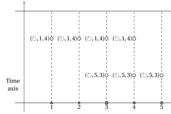
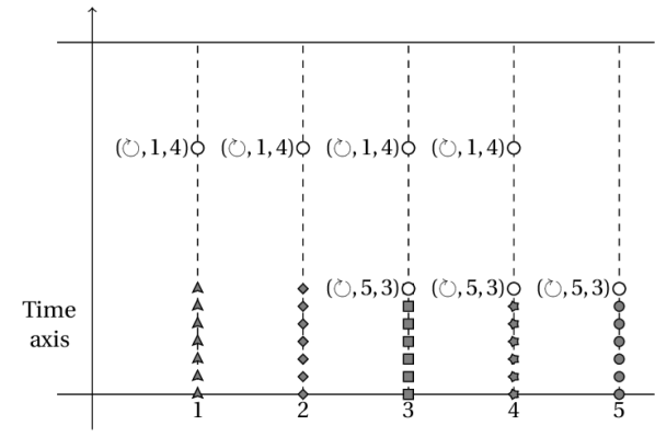
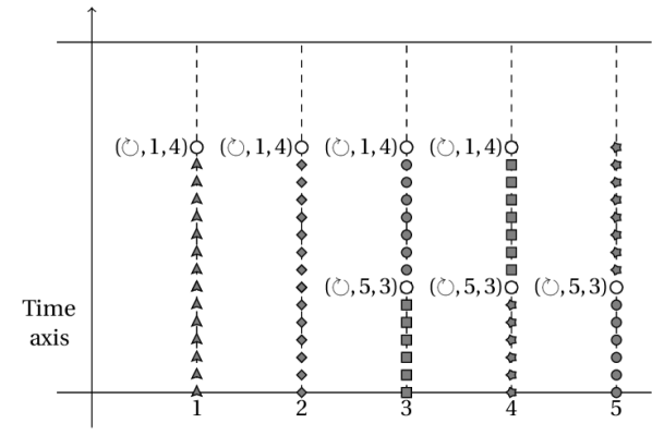
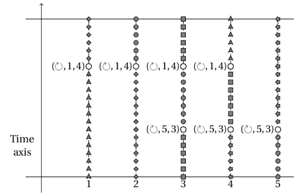
Figure 3: Evolution of the sites $1$ to $5$ under pregenerator $\mathscr{L}_{2}$ given a realization of the marked PPPs. It should be read by line from the left to the right. Here, stands for $\mathtt{a}$, for $\mathtt{t}$, for $\mathtt{c}$ and for $\mathtt{g}$.

5.1.3 Construction of the dual process

Thanks to the constructions provided in Sections 5.1.1 and 5.1.2, to have a graphical representation of the process with pregenerator $\mathscr{L}$, it suffices to multiply the rates of $\mathscr{N}$ by $\rho$, and to assume that ${\mathfrak{M}}$, ${\mathfrak{M}}^{0}$, $\mathscr{U}$, $\mathscr{U}^{0}$ and $\mathscr{N}$, are mutually independent.

Now, we turn to the construction of the generalized dual process of $\mathscr{L}$. It is a marked branching structure constructed on the space ${\mathbb{Z}}\times[0,+\infty)$.

Fix a finite set of sites $D\subset{\mathbb{Z}}$ and a time $t$. Suppose that for the time interval $[0,t]$, we have a realization $\omega$ of the marked PPPs described above. We reverse the time direction calling $\widehat{u}=t-u$ and we construct a space-time branching structure contained in ${\mathbb{Z}}\times[\widehat{0},\widehat{t}]$ with base $(D,\widehat{0})$ and top $(D_{\widehat{t}},\widehat{t})$. We proceed by induction with the following recipe.

Suppose that the spatial projection of the structure at time $\widehat{u}$ is $D_{\widehat{u}}$. Let $\widehat{T}$ be the first Poisson mark after $\widehat{u}$ involving some site of $D_{\widehat{u}}$. There are the following possibilities.

• A $(j,a)$-mark involving site $x\in D_{\widehat{T}^{-}}$ with $j\in J(a)\setminus\{0\}$. In this case, the point $(x,\widehat{T})$ is marked $(j,a)$ and the set $D_{\widehat{T}}$ will be $D_{\widehat{T}^{-}}\cup\Big{(}\bigcup_{\ell\geqslant j}S_{\ell}(x,a)\Big{)}$, where $S_{\ell}(x,a)=\tau_{x}^{-1}S_{\ell}(a)$.

• A $(\delta,a)$-mark involving site $x\in D_{\widehat{T}^{-}}$. In this case, the point $(x,\widehat{T})$ is marked $(\delta,a)$ and the set $D_{\widehat{T}}$ will be $D_{\widehat{T}^{-}}\setminus\{x\}$.

• A $(\circlearrowright,y,z)$-mark involving $x\in D_{\widehat{T}^{-}}$ with $y<z$. In this case, all the points of $D_{\widehat{T}}\cap[y,z]\times\{T\}$ are marked with $(\circlearrowright,y,z)$ and the set $D_{\widehat{T}}$ will be $\sigma_{y,z}^{-1}(D_{\widehat{T}^{-}})=\sigma_{z,y}(D_{\widehat{T}^{-}})$.

• A $(\circlearrowright,y,z)$-mark involving $x\in D_{\widehat{T}^{-}}$ with $y>z$. In this case, all the points of $D_{\widehat{T}}\cap[z,y]\times\{T\}$ are marked with $(\circlearrowright,y,z)$ and the set $D_{\widehat{T}}$ will be $\sigma_{z,y}^{-1}(D_{\widehat{T}^{-}})=\sigma_{y,z}(D_{\widehat{T}^{-}})$.

According to this construction, for each finite set $D$ and time $t$, we are defining a map from the probability space $(\Omega,\mathscr{F},{\mathbb{P}})$ into the space of all possible marked branching structures on ${\mathbb{Z}}\times[\widehat{0},\widehat{t}]$,

$$\widehat{D}_{[\widehat{0},\widehat{t}]}^{D}:(\omega,t)\mapsto\left(N,(\widehat{t}_{k},x_{k},y_{k},z_{k},j_{k},D_{k}),k=1,\dots,N\right),$$ (5.10)

where

• $N$ is the number of marks in the interval $[\widehat{0},\widehat{t}]$,

• $\widehat{t}_{k}$ is the time of the occurrence of the $k$th mark,

• $x_{k}$ is one site involved with the $k$th mark,

• $y_{k}$ and $z_{k}$ are the boundaries of the sites involved with the $k$th mark, if this mark is a circle arrow mark (if not $y_{k}=z_{k}=x_{k}$),

• $j_{k}$ is the type of the $k$th mark ($\delta$, $(j,a)$, or $\circlearrowright$),

• $D_{k}$ is the set of sites in the spatial projection of the structure between times $\widehat{t}_{k}$ and $\widehat{t}_{k+1}$.

Note that there are no ambiguities if at least two sites $x,x^{\prime}\in D_{\widehat{T}^{-}}$ are involved in the same circle arrow mark $(\circlearrowright,y,z)$ with $y<z$. Indeed in both cases, the same set of points are marked with $(\circlearrowright,y,z)$ and the set $D_{\widehat{T}}$ will be $\sigma_{y,z}^{-1}(D_{\widehat{T}^{-}})$. It is similar with a circle arrow mark $(\circlearrowright,y,z)$ with $y>z$.

One can check that if $D$ and $D^{\prime}$ are finite sets of sites such that $D\subset D^{\prime}$, then the marked branching structure

$$\widehat{D}_{[\widehat{0},\widehat{t}]}^{D}(\omega,t)=\left(N,(\widehat{t}_{k},x_{k},y_{k},z_{k},j_{k},D_{k}),k=1,\dots,N\right)$$

is a subset of the marked branching structure

$$\widehat{D}_{[\widehat{0},\widehat{t}]}^{D^{\prime}}(\omega,t)=\left(N^{\prime},(\widehat{t}^{\prime}_{k},x^{\prime}_{k},y^{\prime}_{k},z^{\prime}_{k},j^{\prime}_{k},D^{\prime}_{k}),k=1,\dots,N^{\prime}\right),$$

in the sense that $N\leqslant N^{\prime}$, and for any $k$ in $\{1,\dots,N\}$, there exists $r(k)$ in $\{1,\dots,N^{\prime}\}$ such that

$$(\widehat{t}_{k},x_{k},y_{k},z_{k},j_{k})=(\widehat{t}^{\prime}_{r(k)},x^{\prime}_{r(k)},y^{\prime}_{r(k)},z^{\prime}_{r(k)},j^{\prime}_{r(k)})\quad\mbox{and}\quad D_{k}\subset D^{\prime}_{r(k)}.$$

The central idea of the construction is exactly the same as in [Fer90]: when we go back in time and the generalized dual process meets a $(\delta,a)$-mark at site $x$, it is not necessary to go further to know the value of $\eta(x)$, because it is determined at that point by an independent random variable.

5.2 Proofs of Theorems 3.1 and 3.4, and of Remarks 3.2(i) and 3.5(i)

Proof.

(of Theorem 3.1). The proof is adapted from [Fer90]. If the spatial projection of the dual structure started at time $t=\widehat{0}$ is empty at time $0=\widehat{t}$, that is, $D_{\widehat{t}}^{D}=\emptyset$, then $\eta_{t}(D)$ does not depend on $\eta_{0}=\eta$. This implies that a sufficient condition for the exponential ergodicity of the process is that, for all finite set $D$, there exists positive constants $\alpha_{1}$, $\alpha_{2}$ such that

$${\mathbb{P}}(D_{\widehat{t}}^{D}=\emptyset)\leqslant\alpha_{1}|D|\mathrm{e}^{-t\alpha_{2}}.$$ (5.11)

Hence, we are interested in the evolution of the cardinal of $D_{\widehat{u}}^{D}$. Since the marks coming from the cut-and-paste process do not change the cardinal of $D_{\widehat{u}}^{D}$ along time, they are not involved in the following.

The process $|D_{\widehat{u}}^{D}|$ can be dominated by a branching process $Z_{u}^{|D|}\in{\mathbb{N}}$, that is, $|D_{\widehat{u}}^{D}|\leqslant Z_{u}^{|D|}$ for all $u$ with probability one. This branching process is defined as follows. At rate $\overline{\lambda}+\overline{\lambda}_{0}$ (defined in (3.6) and (3.5)) each branch dies and is replaced by either $s$ new branches with probability $\overline{\lambda}/(\overline{\lambda}+\overline{\lambda}_{0})$ or $0$ new branches with probability $\overline{\lambda}_{0}/(\overline{\lambda}+\overline{\lambda}_{0})$.

Indeed, in the generalized dual process presented in Section 5.1.3, a site $x$ is removed from $D_{\widehat{u}}^{D}$ at time $\widehat{T}$ when a $(\delta,a)$-mark appears at $(x,\widehat{T})$. The $(\delta,a)$-marks are distributed according to a PPP with rate $\lambda_{0}(a)$. Therefore, the total rate at which site $x$ is removed from $D_{\widehat{u}}^{D}$ is $\sum_{a\in\mathscr{A}}\lambda_{0}(a)=\overline{\lambda}_{0}$. Hence in the dominating branching process, a branch dies at rate $\overline{\lambda}_{0}$.

Now, we focus on the apparition of new branches. In the generalized dual process, when a $(j,a)$-mark appears at $(x,\widehat{T})$, a maximum number of $|\bigcup_{\ell\geqslant j}S_{j}(x,a)|=s_{j}(a)$ sites might be added to $D_{\widehat{u}}^{D}$. This happens at rate $\overline{\lambda}_{j}(a)$. Therefore for the dominating branching process, we use the bounds $\overline{\lambda}_{j}(a)\leqslant\overline{\lambda}$ and $s_{j}(a)\leqslant s$, so that a branch is replaced by $s$ branches at rate $\overline{\lambda}$.

The initial state of the branching process is $Z_{0}^{|D|}=|D|$. A sufficient condition for (5.11) is that the average number of branches created at each branching is less than $1$. This happens when

$$\frac{s\overline{\lambda}}{\overline{\lambda}+\overline{\lambda}_{0}}<1.$$ (5.12)

∎

Proof.

(of Theorem 3.4). The construction in this case of the generalized dual process follows the line of construction in Section 5.1.3, except that one should replace 1(a) by

• A $(j,a,i)$-mark involving site $x\in D_{\widehat{T}^{-}}$ with $j\in J^{(i)}(x,a)\setminus\{0\}$. In this case, the point $(x,\widehat{T})$ is marked $(j,a,i)$ and the set $D_{\widehat{T}}$ will be $D_{\widehat{T}^{-}}\cup S^{(i)}(x,a)$, where $S^{(i)}(x,a)=\tau_{x}^{-1}S^{(i)}(a)$.

To prove (3.7) in Theorem 3.1, we said that a branch in the dominating branching process dies and is either replaced by $s$ or $0$ branches. To prove here (3.16) we say that a branch in the dominating branching process dies at rate $\Theta=\overline{\lambda}_{0,d}+\sum_{i=1}^{d}\overline{\lambda}^{(i)}$ (recall (3.14) and (3.15)), and is either replaced by $s^{(1)}$, $\dots$, $s^{(d)}$ or $0$ branches at respective rates $\overline{\lambda}^{(1)}/\Theta$, $\dots$, $\overline{\lambda}^{(d)}/\Theta$ and $\overline{\lambda}_{0,d}/\Theta$.

A sufficient condition for (5.11) is now

$$\sum_{i=1}^{d}\frac{s^{(i)}\overline{\lambda}^{(i)}}{\Theta}<1,$$ (5.13)

which is equivalent to (3.16). ∎

Proof.

(of Remarks 3.2(i) and 3.5(i)). To recover analogous results to Theorems 2.1 and 2.2 in [Fer90] requires two main changes in the steps to prove Theorems 3.1 and 3.4: We have to take a ‘uniform noise’ when rewriting the generator $\mathscr{L}_{1}$, then to take a different bound to define the birth rates of the branching process. We define the quantities we have to modify with an upper index F (we keep the other ones unchanged), and consider in parallel the two results.

We have to replace the definitions of $\overline{\lambda}_{0}(a)$ in (3.3), and of $\overline{\lambda}_{0}^{(i)}(a)$ in (3.11), by

$$\overline{\lambda}_{0}^{\textsc{F}}(a)=\lambda_{0}(a)-m,\qquad\overline{\lambda}_{0}^{(i),{\textsc{F}}}(a)=\lambda_{0}^{(i)}(a)-m^{(i)},$$ (5.14)

the one of $\lambda(a)$ in (3.4), and of $\lambda^{(i)}(a)$ in (3.12), by

$$\lambda^{\textsc{F}}(a) = \max\big{\{}\lambda_{j}(a)\,:\,j\in J(a)\big{\}}-m=\lambda_{|J(a)|-1}-m,$$ (5.15)

$$\lambda^{(i),{\textsc{F}}}(a) = \max\big{\{}\lambda_{j}^{(i)}(a)\,:\,j\in J^{(i)}(a)\big{\}}-m^{(i)}=\lambda^{(i)}_{|J^{(i)}(a)|-1}-m^{(i)};$$ (5.16)

also take, instead of (3.5) and of (3.14),

$$\overline{\lambda}_{0}^{\textsc{F}}=|\mathscr{A}|m,\qquad\overline{\lambda}_{0,d}^{\textsc{F}}=|\mathscr{A}|\sum_{i=1}^{d}m^{(i)},$$ (5.17)

and, instead of (3.6) and of (3.15),

$$\overline{\lambda}^{\textsc{F}} = \max_{a\in\mathscr{A}}\Big{(}\overline{\lambda}_{0}^{\textsc{F}}(a)+\sum_{j\in J(a)\setminus\{0\}}\overline{\lambda}_{j}(a)\Big{)}=\max_{a\in\mathscr{A}}\lambda^{\textsc{F}}(a)=K-m,$$ (5.18)

$$\overline{\lambda}^{(i),{\textsc{F}}} = \max_{a\in\mathscr{A}}\Big{(}\overline{\lambda}_{0}^{(i),{\textsc{F}}}(a)+\sum_{j\in J^{(i)}(a)\setminus\{0\}}\overline{\lambda}_{j}^{(i)}(a)\Big{)}=\max_{a\in\mathscr{A}}\lambda^{(i),{\textsc{F}}}(a)=K^{(i)}-m^{(i)}.$$ (5.19)

Then, instead of (5.2) and of (5.6), rewrite the pregenerator $\mathscr{L}_{1}$ as

$$\mathscr{L}_{1}f(\eta) = \sum_{x\in{\mathbb{Z}}}\sum_{a\in\mathscr{A}}\sum_{j\in J(a)\setminus\{0\}}\overline{\lambda}_{j}(a)\sum_{\ell\geqslant j}{\mathbf{1}}_{\{\eta\in A_{\ell}(x,a)\}}\big{[}f(\eta^{x}_{a})-f(\eta)\big{]}$$ (5.20)

$$+\sum_{x\in{\mathbb{Z}}}\sum_{a\in\mathscr{A}}\overline{\lambda}_{0}^{\textsc{F}}(a)\sum_{\ell\geqslant 0}{\mathbf{1}}_{\{\eta\in A_{\ell}(x,a)\}}\big{[}f(\eta^{x}_{a})-f(\eta)\big{]}$$

$$+\sum_{x\in{\mathbb{Z}}}\overline{\lambda}_{0}^{\textsc{F}}\sum_{a\in\mathscr{A}}\frac{1}{|\mathscr{A}|}\left[f(\eta^{x}_{a})-f(\eta)\right].$$

and

$$\mathscr{L}_{1}f(\eta) = \sum_{i=1}^{d}\sum_{x\in{\mathbb{Z}}}\sum_{a\in\mathscr{A}}\sum_{j\in J^{(i)}(a)\setminus\{0\}}\overline{\lambda}_{j}^{(i)}(a)\sum_{\ell\geqslant j}{\mathbf{1}}_{\{\eta\in A_{\ell}^{(i)}(x,a)\}}\big{[}f(\eta^{x}_{a})-f(\eta)\big{]}$$ (5.21)

$$+\sum_{i=1}^{d}\sum_{x\in{\mathbb{Z}}}\sum_{a\in\mathscr{A}}\overline{\lambda}_{0}^{(i),{\textsc{F}}}(a)\sum_{\ell\geqslant 0}{\mathbf{1}}_{\{\eta\in A_{\ell}^{(i)}(x,a)\}}\big{[}f(\eta^{x}_{a})-f(\eta)\big{]}$$

$$+\sum_{x\in{\mathbb{Z}}}\overline{\lambda}_{0,d}^{\textsc{F}}\sum_{a\in\mathscr{A}}\frac{1}{|\mathscr{A}|}\left[f(\eta^{x}_{a})-f(\eta)\right].$$

In the graphical construction, replace the definitions (5.5) and (5.9) by

$${\mathbb{P}}(U^{0,{\textsc{F}}}_{n}(x)=a)=\frac{1}{|\mathscr{A}|};\qquad{\mathbb{P}}(U^{0,d,{\textsc{F}}}_{n}(x)=a)=\frac{1}{|\mathscr{A}|},$$ (5.22)

so that these discrete random variables become uniform. Finally, the conditions for extinction (5.12) and (5.13) become

$$\frac{s\overline{\lambda}^{\textsc{F}}}{\overline{\lambda}^{\textsc{F}}+\overline{\lambda}_{0}^{\textsc{F}}}<1,\qquad\frac{\sum_{i=1}^{d}s^{(i)}\overline{\lambda}^{(i),{\textsc{F}}}}{\overline{\lambda}_{0,d}^{\textsc{F}}+\sum_{i=1}^{d}\overline{\lambda}^{(i),{\textsc{F}}}}<1.$$ (5.23)

∎

6 Proofs through attractiveness

Proof.

(of Proposition 4.1). The lower and upper invariant probability measures are $\mu_{l}=\lim_{t\to\infty}\delta_{\underline{\mathtt{c}}}S(t)$ and $\mu_{u}=\lim_{t\to\infty}\delta_{\underline{\mathtt{g}}}S(t)$, where $\delta_{\underline{\mathtt{c}}}$ (resp. $\delta_{\underline{\mathtt{g}}}$) denotes the Dirac measure on the configuration $\eta$ such that $\eta(x)=\mathtt{c}$ (resp. $\eta(x)=\mathtt{g}$) for all $x\in{\mathbb{Z}}$. They are translation invariant. To prove ergodicity, we have to show that $\mu_{l}=\mu_{u}$.

$\bullet$ Step 1: We derive consequences of attractiveness.
Note that the functions $\phi(\eta)={\mathbf{1}}_{\{\eta(0)\geqslant\mathtt{g}\}}$ and $\varphi(\eta)={\mathbf{1}}_{\{\eta(0)>\mathtt{c}\}}$ belong to $\mathscr{M}$, and since $\mathtt{c}$ and $\mathtt{g}$ are respectively the smallest and largest elements of $\mathscr{A}$ with respect to the order (4.1), we have $\phi(\eta)={\mathbf{1}}_{\{\eta(0)=\mathtt{g}\}}$ and $\varphi(\eta)=1-{\mathbf{1}}_{\{\eta(0=\mathtt{c}\}}$, hence

$$\mu_{l}(\eta(0)=\mathtt{g})\leqslant\mu_{u}(\eta(0)=\mathtt{g})\qquad\mbox{and}\qquad\mu_{u}(\eta(0)=\mathtt{c})\leqslant\mu_{l}(\eta(0)=\mathtt{c}).$$ (6.1)

Similarly, the function $\psi(\eta)={\mathbf{1}}_{\{\eta(0)>\mathtt{t}\}}$ belongs to $\mathscr{M}$, and, by the order (4.1), it satisfies $\psi(\eta)={\mathbf{1}}_{\{\eta(0)=\mathtt{a}\}}+{\mathbf{1}}_{\{\eta(0)=\mathtt{g}\}}=1-{\mathbf{1}}_{\{\eta(0)=\mathtt{c}\}}-{\mathbf{1}}_{\{\eta(0)=\mathtt{t}\}}$. We thus have that

$$\mu_{l}(\eta(0)=\mathtt{a})+\mu_{l}(\eta(0)=\mathtt{g}) \leqslant \mu_{u}(\eta(0)=\mathtt{a})+\mu_{u}(\eta(0)=\mathtt{g}),$$ (6.2)

$$\mu_{l}(\eta(0)=\mathtt{c})+\mu_{l}(\eta(0)=\mathtt{t}) \geqslant \mu_{u}(\eta(0)=\mathtt{c})+\mu_{u}(\eta(0)=\mathtt{t}).$$ (6.3)

$\bullet$ Step 2: We take into account the assumptions on the rates.
Combining (6.1) with (4.3) implies

$$\mu_{l}(\eta(0)=\mathtt{c})=\mu_{u}(\eta(0)=\mathtt{c})=\mu_{l}(\eta(0)=\mathtt{g})=\mu_{u}(\eta(0)=\mathtt{g}).$$ (6.4)

Then combining (6.4) first with (6.2), and then with (6.3) yields

$$\mu_{l}(\eta(0)=\mathtt{a}) \leqslant \mu_{u}(\eta(0)=\mathtt{a}),$$ (6.5)

$$\mu_{l}(\eta(0)=\mathtt{t}) \geqslant \mu_{u}(\eta(0)=\mathtt{t}).$$ (6.6)

Finally, combining (6.5)–(6.6) with (4.2) implies

$$\mu_{l}(\eta(0)=\mathtt{t})=\mu_{u}(\eta(0)=\mathtt{t})=\mu_{l}(\eta(0)=\mathtt{a})=\mu_{u}(\eta(0)=\mathtt{a}).$$ (6.7)

$\bullet$ Step 3: We now proceed in the same spirit as in Corollary II.2.8 in [Lig05]. Let $\nu$ be a monotone coupling measure of $\mu_{l}$ and $\mu_{u}$. It thus has to satisfy

$$\nu((\eta,\xi):\eta(0)\neq\xi(0))=\nu((\eta(0),\xi(0))\in\{(\mathtt{c},\mathtt{t}),(\mathtt{c},\mathtt{a}),(\mathtt{c},\mathtt{g}),(\mathtt{t},\mathtt{a}),(\mathtt{t},\mathtt{g}),(\mathtt{a},\mathtt{g})\}),$$ (6.8)

so that by (6.4),

$$\nu((\eta,\xi):\eta(0)=\xi(0)=\mathtt{g}) = \mu_{l}(\eta(0)=\mathtt{g})=\mu_{u}(\xi(0)=\mathtt{g}),$$ (6.9)

$$\nu((\eta,\xi):\eta(0)=\xi(0)=\mathtt{c}) = \mu_{u}(\xi(0)=\mathtt{c})=\mu_{l}(\eta(0)=\mathtt{c}).$$ (6.10)

By (6.8), (6.9) and (6.10), and because $\mathtt{c}$ and $\mathtt{g}$ are respectively the smallest and largest elements of $\mathscr{A}$ with respect to the order (4.1),

$$\nu((\eta,\xi):\eta(0)\not=\mathtt{g},\xi(0)=\mathtt{g}) = \nu((\eta(0),\xi(0))\in\{(\mathtt{c},\mathtt{g}),(\mathtt{t},\mathtt{g}),(\mathtt{a},\mathtt{g})\})$$

$$= \mu_{u}(\xi(0)=\mathtt{g})-\nu(\eta(0)=\xi(0)=\mathtt{g})=0,$$ (6.11)

$$\nu((\eta,\xi):\eta(0)=\mathtt{c},\xi(0)\not=\mathtt{c}) = \nu((\eta(0),\xi(0))\in\{(\mathtt{c},\mathtt{t}),(\mathtt{c},\mathtt{a}),(\mathtt{c},\mathtt{g})\})$$ (6.12)

$$= \mu_{l}(\eta(0)=\mathtt{c})-\nu(\eta(0)=\xi(0)=\mathtt{c})=0,$$

so that, using also again (6.8) with respectively (6.12) and (6.11), we obtain,

$$\nu((\eta,\xi):\eta(0)\not=\mathtt{a},\xi(0)=\mathtt{a}) = \nu((\eta(0),\xi(0))\in\{(\mathtt{c},\mathtt{a}),(\mathtt{t},\mathtt{a})\})$$ (6.13)

$$= 0+\nu(\eta(0)=\mathtt{t},\xi(0)=\mathtt{a}),$$

$$\nu((\eta,\xi):\eta(0)=\mathtt{a},\xi(0)\not=\mathtt{a}) = \nu((\eta(0),\xi(0))=(\mathtt{a},\mathtt{g}))=0.$$ (6.14)

Since we also have

$$\nu((\eta,\xi):\eta(0)\not=\mathtt{a},\xi(0)=\mathtt{a}) = \mu_{u}(\xi(0)=\mathtt{a})-\nu(\eta(0)=\xi(0)=\mathtt{a}),$$ (6.15)

$$\nu((\eta,\xi):\eta(0)=\mathtt{a},\xi(0)\not=\mathtt{a}) = \mu_{l}(\eta(0)=\mathtt{a})-\nu(\eta(0)=\xi(0)=\mathtt{a}),$$ (6.16)

combining (6.13), (6.14) with (6.7) implies that

$$\nu(\eta(0)=\mathtt{t},\xi(0)=\mathtt{a})=0.$$ (6.17)

Note that all the possible cases on the r.h.s. of (6.8) have probability $0$: $(\mathtt{c},\mathtt{g}),(\mathtt{t},\mathtt{g}),(\mathtt{a},\mathtt{g})$ by (6.11), $(\mathtt{c},\mathtt{t}),(\mathtt{c},\mathtt{a})$ by (6.12), $(\mathtt{t},\mathtt{a})$ by (6.17). We conclude that

$$\nu((\eta,\xi):\eta(0)\neq\xi(0))=0,$$

hence $\mu_{l}=\mu_{u}$. ∎

$\bullet$ Monotonicity of the RN+YpR model, and of the RN+YpR model with cut-and-paste mechanism

Proof.

(of Proposition 4.3). We denote by $\overline{\mathscr{L}_{1}}$ the pregenerator of the monotone coupled dynamics for the RN+YpR substitution process (which exists by our assumption). Let similarly $\overline{\mathscr{L}}_{2}$ denote the pregenerator of the coupled cut-and-paste dynamics through basic coupling, that is, the same transition takes place for both copies of the process: it is defined by, for a cylinder function $g$ on $X\times X$,

$$\overline{\mathscr{L}}_{2}g(\eta,\xi)=\sum_{x,y\in{\mathbb{Z}}}p(x,y)\big{[}g(\sigma_{x,y}(\eta),\sigma_{x,y}(\xi))-g(\eta,\xi)\big{]}.$$ (6.18)

This coupled dynamics is monotone, since a transition does not change the way in which the values of the two processes on each site are coupled. For the complete dynamics (that is the RN+YpR model with cut-and-paste mechanism) we consider the combination of both couplings, that is the pregenerator

$$\overline{\mathscr{L}}g=\overline{\mathscr{L}}_{1}g+\rho\overline{\mathscr{L}}_{2}g.$$ (6.19)

Being the sum of two pregenerators of attractive dynamics, it yields also an attractive dynamics. We denote by $(\overline{S}(t),t\geqslant 0)$ its semi-group. ∎

Proof.

(of Proposition 4.4). To derive attractiveness, we construct a coupled dynamics $(\eta_{t},\xi_{t})_{t\geqslant 0}$ starting from ordered configurations $\eta_{0}\leqslant\xi_{0}$, through basic coupling. Then we find conditions on the rates prohibiting the coupled transitions breaking the increasing order between coupled configurations. We will denote by $\overline{\mathscr{L}}_{1}$ the induced coupled generator (its existence was assumed in Proposition 4.3). Similarly with (2.1), this generator is defined on a cylinder function $f$ on $X\times X$ by

$$\overline{\mathscr{L}}_{1}f(\eta,\xi)=\sum_{x\in{\mathbb{Z}}}\sum_{(a,b)\in\mathscr{A}\times\mathscr{A}}\ \overline{c}((a,b),\tau_{x}(\eta,\xi))\big{[}f(\eta^{x}_{a},\xi^{x}_{b})-f(\eta,\xi)\big{]}.$$ (6.20)

We now define the coupled rates $\overline{c}((a,b),\tau_{x}(\eta,\xi))$ for the transitions $(\eta,\xi)\to(\eta^{x}_{a},\xi^{x}_{b})$.

By translation invariance of the dynamics, it is enough to look at site 0. Thus we write the coupled transitions and their rates (according to basic coupling) in the following 3 tables. There, we indicate with the symbol $(*)$ the coupled transitions to be forbidden for attractiveness; we derive after each table the corresponding sufficient conditions that these forbidden interactions induce.

We rely on the rates given in Table 1 for the RN+YpR model.

$$\begin{array}[]{lll|l}\lx@intercol\hfil\mbox{Transition}\hfil\lx@intercol\vrule\lx@intercol&\lx@intercol\hfil\mbox{Rate}\hfil\lx@intercol\\ \hline\cr\hline\cr(\mathtt{c},\mathtt{c})&\to&(\mathtt{a},\mathtt{a})&v_{\mathtt{a}}\\ &\to&(\mathtt{g},\mathtt{g})&v_{\mathtt{g}}\\ &\to&(\mathtt{t},\mathtt{t})&\min\{c(\mathtt{t},\eta),c(\mathtt{t},\xi)\}\\ &\to&(\mathtt{c},\mathtt{t})&c(\mathtt{t},\xi)-\min\{c(\mathtt{t},\eta),c(\mathtt{t},\xi)\}\\ &\to&(\mathtt{t},\mathtt{c})\quad(*)&c(\mathtt{t},\eta)-\min\{c(\mathtt{t},\eta),c(\mathtt{t},\xi)\}\\ \hline\cr(\mathtt{c},\mathtt{t})&\to&(\mathtt{a},\mathtt{a})&v_{\mathtt{a}}\\ &\to&(\mathtt{g},\mathtt{g})&v_{\mathtt{g}}\\ &\to&(\mathtt{t},\mathtt{t})&c(\mathtt{t},\eta)\\ &\to&(\mathtt{c},\mathtt{c})&c(\mathtt{c},\xi)\\ \hline\cr(\mathtt{c},\mathtt{a})&\to&(\mathtt{a},\mathtt{a})&v_{\mathtt{a}}\\ &\to&(\mathtt{t},\mathtt{t})&v_{\mathtt{t}}\\ &\to&(\mathtt{t},\mathtt{a})&c(\mathtt{t},\eta)-v_{\mathtt{t}}\\ &\to&(\mathtt{c},\mathtt{c})&v_{\mathtt{c}}\\ &\to&(\mathtt{g},\mathtt{g})&v_{\mathtt{g}}\\ &\to&(\mathtt{c},\mathtt{g})&c(\mathtt{g},\xi)-v_{\mathtt{g}}\\ \hline\cr(\mathtt{c},\mathtt{g})&\to&(\mathtt{a},\mathtt{a})&v_{\mathtt{a}}\\ &\to&(\mathtt{c},\mathtt{a})&c(\mathtt{a},\xi)-v_{\mathtt{a}}\\ &\to&(\mathtt{t},\mathtt{t})&v_{\mathtt{t}}\\ &\to&(\mathtt{t},\mathtt{g})&c(\mathtt{t},\eta)-v_{\mathtt{t}}\\ &\to&(\mathtt{c},\mathtt{c})&v_{\mathtt{c}}\\ &\to&(\mathtt{g},\mathtt{g})&v_{\mathtt{g}}\\ \end{array}$$

Under basic coupling, both configurations undergo the same transition according to the maximal possible rate, and then uncoupled transitions are added to fit the correct transitions for each marginal. We detail this construction in the first 5 lines of this first table, the others are similar. There, we start from $(\eta(0),\xi(0))=(\mathtt{c},\mathtt{c})$. The rate for a transition from $\mathtt{c}$ to $\mathtt{a}$ or to $\mathtt{g}$ in Table 1 does not depend on the value of the configuration on neighboring sites, therefore here we have transitions respectively to $(\mathtt{a},\mathtt{a})$ or $(\mathtt{g},\mathtt{g})$ with the rates $v_{\mathtt{a}}$ or $v_{\mathtt{g}}$, and these rates yield the correct rate for each marginal transition. But the rate for a transition from $\mathtt{c}$ to $\mathtt{t}$ in Table 1 depends on the value of the configuration on site $1$. Therefore the maximal rate for a coupled transition from $(\mathtt{c},\mathtt{c})$ to $(\mathtt{t},\mathtt{t})$ is $\min\{c(\mathtt{t},\eta),c(\mathtt{t},\xi)\}$, and, to obtain the correct rate for each marginal transition, it has to be supplemented by respective uncoupled transitions to $(\mathtt{c},\mathtt{t})$ and $(\mathtt{t},\mathtt{c})$, with rates $c(\mathtt{t},\xi)-\min\{c(\mathtt{t},\eta),c(\mathtt{t},\xi)\}$ and $c(\mathtt{t},\eta)-\min\{c(\mathtt{t},\eta),c(\mathtt{t},\xi)\}$.

But a transition to $(\mathtt{t},\mathtt{c})$ would break the increasing order between the coupled configurations. To forbid it, that is, for its rate to be 0, we need to have

$$c(\mathtt{t},\eta)=\min\{c(\mathtt{t},\eta),c(\mathtt{t},\xi)\}.$$ (6.21)

There are two possibilities, according to the value of the coupled configuration on $1$, which is such that $\eta(1)\leqslant\xi(1)$. Either $\eta(1)\in Y=\{\mathtt{c},\mathtt{t}\}$, hence $c(\mathtt{t},\eta)=w_{\mathtt{t}}\leqslant c(\mathtt{t},\xi)$, and (6.21) is satisfied; or $\eta(1)\in R=\{\mathtt{a},\mathtt{g}\}$, hence $c(\mathtt{t},\eta)=w_{\mathtt{t}}+r_{\mathtt{t}}^{\eta(1)}$ and $c(\mathtt{t},\xi)=w_{\mathtt{t}}+r_{\mathtt{t}}^{\xi(1)}$: a necessary and sufficient condition for (6.21) to be satisfied is

$$r_{\mathtt{t}}^{\mathtt{a}}\leqslant r_{\mathtt{t}}^{\mathtt{g}}.$$

$$\begin{array}[]{lll|l}\lx@intercol\hfil\mbox{Transition}\hfil\lx@intercol\vrule\lx@intercol&\lx@intercol\hfil\mbox{Rate}\hfil\lx@intercol\\ \hline\cr\hline\cr(\mathtt{t},\mathtt{t})&\to&(\mathtt{a},\mathtt{a})&v_{\mathtt{a}}\\ &\to&(\mathtt{c},\mathtt{c})&\min\{c(\mathtt{c},\eta),c(\mathtt{c},\xi)\}\\ &\to&(\mathtt{c},\mathtt{t})&c(\mathtt{c},\eta)-\min\{c(\mathtt{c},\eta),c(\mathtt{c},\xi)\}\\ &\to&(\mathtt{t},\mathtt{c})\quad(*)&c(\mathtt{c},\xi)-\min\{c(\mathtt{c},\eta),c(\mathtt{c},\xi)\}\\ &\to&(\mathtt{g},\mathtt{g})&v_{\mathtt{g}}\\ \hline\cr(\mathtt{t},\mathtt{a})&\to&(\mathtt{a},\mathtt{a})&v_{\mathtt{a}}\\ &\to&(\mathtt{t},\mathtt{t})&v_{\mathtt{t}}\\ &\to&(\mathtt{c},\mathtt{c})&v_{\mathtt{c}}\\ &\to&(\mathtt{c},\mathtt{a})&c(\mathtt{c},\eta)-v_{\mathtt{c}}\\ &\to&(\mathtt{g},\mathtt{g})&v_{\mathtt{g}}\\ &\to&(\mathtt{t},\mathtt{g})&c(\mathtt{g},\xi)-v_{\mathtt{g}}\\ \hline\cr(\mathtt{t},\mathtt{g})&\to&(\mathtt{a},\mathtt{a})&v_{\mathtt{a}}\\ &\to&(\mathtt{t},\mathtt{a})&c(\mathtt{a},\xi)-v_{\mathtt{a}}\\ &\to&(\mathtt{c},\mathtt{c})&v_{\mathtt{c}}\\ &\to&(\mathtt{c},\mathtt{g})&c(\mathtt{c},\eta)-v_{\mathtt{c}}\\ &\to&(\mathtt{t},\mathtt{t})&v_{\mathtt{t}}\\ &\to&(\mathtt{g},\mathtt{g})&v_{\mathtt{g}}\\ \end{array}$$

In this second table, the transition from $(\mathtt{t},\mathtt{t})$ to $(\mathtt{t},\mathtt{c})$ has to be forbidden for attractiveness, which requires

$$c(\mathtt{c},\xi)=\min\{c(\mathtt{c},\eta),c(\mathtt{c},\xi)\}.$$ (6.22)

We have that

$$c(\mathtt{c},\eta)=w_{\mathtt{c}}+r_{\mathtt{c}}^{\eta(1)}{\mathbf{1}}_{\{\eta(1)\in R\}},\quad c(\mathtt{c},\xi)=w_{\mathtt{c}}+r_{\mathtt{c}}^{\xi(1)}{\mathbf{1}}_{\{\xi(1)\in R\}},\quad\mbox{with}\quad\eta(1)\leqslant\xi(1).$$

Thus (6.22) is satisfied if and only if

$$r_{\mathtt{c}}^{\mathtt{a}}=r_{\mathtt{c}}^{\mathtt{g}}=0.$$

$$\begin{array}[]{lll|l}\lx@intercol\hfil\mbox{Transition}\hfil\lx@intercol\vrule\lx@intercol&\lx@intercol\hfil\mbox{Rate}\hfil\lx@intercol\\ \hline\cr\hline\cr(\mathtt{a},\mathtt{a})&\to&(\mathtt{t},\mathtt{t})&v_{\mathtt{t}}\\ &\to&(\mathtt{c},\mathtt{c})&v_{\mathtt{c}}\\ &\to&(\mathtt{g},\mathtt{g})&\min\{c(\mathtt{g},\eta),c(\mathtt{g},\xi)\}\\ &\to&(\mathtt{a},\mathtt{g})&c(\mathtt{g},\xi)-\min\{c(\mathtt{g},\eta),c(\mathtt{g},\xi)\}\\ &\to&(\mathtt{g},\mathtt{a})\quad(*)&c(\mathtt{g},\eta)-\min\{c(\mathtt{g},\eta),c(\mathtt{g},\xi)\}\\ \hline\cr(\mathtt{a},\mathtt{g})&\to&(\mathtt{a},\mathtt{a})&c(\mathtt{a},\xi)\\ &\to&(\mathtt{g},\mathtt{g})&c(\mathtt{g},\eta)\\ &\to&(\mathtt{t},\mathtt{t})&v_{\mathtt{t}}\\ &\to&(\mathtt{c},\mathtt{c})&v_{\mathtt{c}}\\ \hline\cr(\mathtt{g},\mathtt{g})&\to&(\mathtt{a},\mathtt{a})&\min\{c(\mathtt{a},\eta),c(\mathtt{a},\xi)\}\\ &\to&(\mathtt{a},\mathtt{g})&c(\mathtt{a},\eta)-\min\{c(\mathtt{a},\eta),c(\mathtt{a},\xi)\}\\ &\to&(\mathtt{g},\mathtt{a})\quad(*)&c(\mathtt{a},\xi)-\min\{c(\mathtt{a},\eta),c(\mathtt{a},\xi)\}\\ &\to&(\mathtt{t},\mathtt{t})&v_{\mathtt{t}}\\ &\to&(\mathtt{c},\mathtt{c})&v_{\mathtt{c}}\\ \end{array}$$

In this third table, the transitions from $(\mathtt{a},\mathtt{a})$ and from $(\mathtt{g},\mathtt{g})$ to $(\mathtt{g},\mathtt{a})$ have to be forbidden for attractiveness, which requires

$$c(\mathtt{g},\eta) = \min\{c(\mathtt{g},\eta),c(\mathtt{g},\xi)\},$$ (6.23)

$$c(\mathtt{a},\xi) = \min\{c(\mathtt{a},\eta),c(\mathtt{a},\xi)\}.$$ (6.24)

We have that

$$c(\mathtt{g},\eta) = w_{\mathtt{g}}+r_{\mathtt{g}}^{\eta(-1)}{\mathbf{1}}_{\{\eta(-1)\in Y\}},\,\,c(\mathtt{g},\xi)=w_{\mathtt{g}}+r_{\mathtt{g}}^{\xi(-1)}{\mathbf{1}}_{\{\xi(-1)\in Y\}},\,\,\mbox{with}\,\,\eta(-1)\leqslant\xi(-1),$$

$$c(\mathtt{a},\eta) = w_{\mathtt{a}}+r_{\mathtt{a}}^{\eta(-1)}{\mathbf{1}}_{\{\eta(-1)\in Y\}},\,\,c(\mathtt{a},\xi)=w_{\mathtt{a}}+r_{\mathtt{a}}^{\xi(-1)}{\mathbf{1}}_{\{\xi(-1)\in Y\}},\,\,\mbox{with}\,\,\eta(-1)\leqslant\xi(-1).$$

Thus (6.23) and (6.24) are respectively satisfied if and only if

$$r_{\mathtt{g}}^{\mathtt{c}}=r_{\mathtt{g}}^{\mathtt{t}} = 0,$$

$$r_{\mathtt{a}}^{\mathtt{t}} \leqslant r_{\mathtt{a}}^{\mathtt{c}}.$$

The proposition is proved. ∎

Proof.

(of Proposition 4.7). We first compute $\mathscr{L}f(\eta)$ for $f(\eta)={\mathbf{1}}_{\{\eta(0)=a\}}$, with $a\in\mathscr{A}$. Recall that we write $c(b,\eta)$ for $c(0,b,\eta)$.

$$\mathscr{L}_{1}f(\eta) = \sum_{b\in\mathscr{A}}c(b,\eta)[f(\eta_{b}^{0})-f(\eta)]$$ (6.25)

$$= -\sum_{b\in\mathscr{A},\,b\not=a}c(b,\eta)f(\eta)+c(a,\eta){\mathbf{1}}_{\{\eta(0)\not=a\}},$$

$$\mathscr{L}_{2}f(\eta) = \sum_{x\in{\mathbb{Z}}}p(x,0)[{\mathbf{1}}_{\{\eta(x)=a\}}-{\mathbf{1}}_{\{\eta(0)=a\}}]+\sum_{x,y\in{\mathbb{Z}},\,x<0<y}p(x,y)[{\mathbf{1}}_{\{\eta(-1)=a\}}-{\mathbf{1}}_{\{\eta(0)=a\}}]$$ (6.26)

$$+\sum_{x,y\in{\mathbb{Z}},\,y<0<x}p(x,y)[{\mathbf{1}}_{\{\eta(1)=a\}}-{\mathbf{1}}_{\{\eta(0)=a\}}].$$

Because $\mu$ is translation invariant, using (6.26), we have that $\int\mathscr{L}_{2}f(\eta)d\mu(\eta)=0$. Therefore, by the invariance of $\mu$, we have $0=\int\mathscr{L}f(\eta)d\mu(\eta)=\int\mathscr{L}_{1}f(\eta)d\mu(\eta)$. Thus we only need to compute $\mathscr{L}_{1}f(\eta)$, relying on the values for the rates given in Table 1, and using (6.25).

$$\mathscr{L}_{1}({\mathbf{1}}_{\{\eta(0)=\mathtt{a}\}}) = -{\mathbf{1}}_{\{\eta(0)=\mathtt{a}\}}(v_{\mathtt{t}}+v_{\mathtt{c}}+w_{\mathtt{g}})-\sum_{a\in Y}{\mathbf{1}}_{\{(\eta(-1),\eta(0))=(a,\mathtt{a})\}}r_{\mathtt{g}}^{a}$$ (6.27)

$$+{\mathbf{1}}_{\{\eta(0)\in Y\}}v_{\mathtt{a}}+{\mathbf{1}}_{\{\eta(0)=\mathtt{g}\}}w_{\mathtt{a}}+\sum_{a\in Y}{\mathbf{1}}_{\{(\eta(-1),\eta(0))=(a,\mathtt{g})\}}r_{\mathtt{a}}^{a},$$

$$\mathscr{L}_{1}({\mathbf{1}}_{\{\eta(0)=\mathtt{g}\}}) = -{\mathbf{1}}_{\{\eta(0)=\mathtt{g}\}}(w_{\mathtt{a}}+v_{\mathtt{t}}+v_{\mathtt{c}})-\sum_{a\in Y}{\mathbf{1}}_{\{(\eta(-1),\eta(0))=(a,\mathtt{g})\}}r_{\mathtt{a}}^{a}$$ (6.28)

$$+{\mathbf{1}}_{\{\eta(0)\in Y\}}v_{\mathtt{g}}+{\mathbf{1}}_{\{\eta(0)=\mathtt{a}\}}w_{\mathtt{g}}+\sum_{a\in Y}{\mathbf{1}}_{\{(\eta(-1),\eta(0))=(a,\mathtt{a})\}}r_{\mathtt{g}}^{a},$$

$$\mathscr{L}_{1}({\mathbf{1}}_{\{\eta(0)=\mathtt{c}\}}) = -{\mathbf{1}}_{\{\eta(0)=\mathtt{c}\}}(v_{\mathtt{a}}+v_{\mathtt{g}}+w_{\mathtt{t}})-\sum_{a\in R}{\mathbf{1}}_{\{(\eta(0),\eta(1))=(\mathtt{c},a)\}}r_{\mathtt{t}}^{a}$$ (6.29)

$$+{\mathbf{1}}_{\{\eta(0)\in R\}}v_{\mathtt{c}}+{\mathbf{1}}_{\{\eta(0)=\mathtt{t}\}}w_{\mathtt{c}}+\sum_{a\in R}{\mathbf{1}}_{\{(\eta(0),\eta(1))=(\mathtt{t},a)\}}r_{\mathtt{c}}^{a},$$

$$\mathscr{L}_{1}({\mathbf{1}}_{\{\eta(0)=\mathtt{t}\}}) = -{\mathbf{1}}_{\{\eta(0)=\mathtt{t}\}}(v_{\mathtt{a}}+w_{\mathtt{c}}+v_{\mathtt{g}})-\sum_{a\in R}{\mathbf{1}}_{\{(\eta(0),\eta(1))=(\mathtt{t},a)\}}r_{\mathtt{c}}^{a}$$ (6.30)

$$+{\mathbf{1}}_{\{\eta(0)\in R\}}v_{\mathtt{t}}+{\mathbf{1}}_{\{\eta(0)=\mathtt{c}\}}w_{\mathtt{t}}+\sum_{a\in R}{\mathbf{1}}_{\{(\eta(0),\eta(1))=(\mathtt{c},a)\}}r_{\mathtt{t}}^{a}.$$

We write $0=\int\mathscr{L}_{1}f(\eta)d\mu(\eta)$ starting from (6.27)–(6.30). This gives the following linear system, whose last line states that $\mu$ is a probability measure.

$$\begin{cases}-(v_{\textsc{y}}+w_{\mathtt{g}})\mu(\eta(0)=\mathtt{a})+w_{\mathtt{a}}\mu(\eta(0)=\mathtt{g})+v_{\mathtt{a}}\mu(Y)&=r_{\textsc{r}},\\ w_{\mathtt{g}}\mu(\eta(0)=\mathtt{a})-(v_{\textsc{y}}+w_{\mathtt{a}})\mu(\eta(0)=\mathtt{g})+v_{\mathtt{g}}\mu(Y)&=-r_{\textsc{r}},\\ -(v_{\textsc{r}}+w_{\mathtt{t}})\mu(\eta(0)=\mathtt{c})+w_{\mathtt{c}}\mu(\eta(0)=\mathtt{t})+v_{\mathtt{c}}\mu(R)&=r_{\textsc{y}},\\ w_{\mathtt{t}}\mu(\eta(0)=\mathtt{c})-(v_{\textsc{r}}+w_{\mathtt{c}})\mu(\eta(0)=\mathtt{t})+v_{\mathtt{t}}\mu(R)&=-r_{\textsc{y}},\\ \mu(\eta(0)=\mathtt{a})+\mu(\eta(0)=\mathtt{g})&=\mu(R),\\ \mu(\eta(0)=\mathtt{c})+\mu(\eta(0)=\mathtt{t})&=\mu(Y),\\ \mu(\eta(0)=\mathtt{a})+\mu(\eta(0)=\mathtt{g})+\mu(\eta(0)=\mathtt{c})+\mu(\eta(0)=\mathtt{t})&=1.\end{cases}$$ (6.31)

Combining the addition of lines 1 and 2 (taking into account lines 5 and 6) with the last line of (6.31) gives a system whose solution is (4.9)–(4.10). We then insert those values into (6.31). Solving the system composed by its lines 1 and 5 (resp. its lines 3 and 6) yields (4.11), (4.13) (resp. (4.12), (4.14)). ∎

Proof.

(of Proposition 4.9). We assume that (4.3) is satisfied; the case where (4.2) is satisfied is similar, and its proof is left to the reader.
We go through the 3 steps of the proof of Proposition 4.1: Step 1 is still valid, with (6.2)–(6.3) which become

$$\mu_{l}(\eta(0)=\mathtt{a})+\mu_{l}(\eta(0)=\mathtt{g}) = \mu_{u}(\eta(0)=\mathtt{a})+\mu_{u}(\eta(0)=\mathtt{g}),$$ (6.32)

$$\mu_{l}(\eta(0)=\mathtt{c})+\mu_{l}(\eta(0)=\mathtt{t}) = \mu_{u}(\eta(0)=\mathtt{c})+\mu_{u}(\eta(0)=\mathtt{t}).$$ (6.33)

because of (4.9)–(4.10). Thus, in Step 2, (6.4) is still valid, as well as (6.5)–(6.6). But combining them with (6.32)–(6.33) implies that

$$\mu_{l}(\eta(0)=\mathtt{t})=\mu_{u}(\eta(0)=\mathtt{t})\quad\hbox{and}\quad\mu_{l}(\eta(0)=\mathtt{a})=\mu_{u}(\eta(0)=\mathtt{a}).$$ (6.34)

Finally, Step 3 is valid, which ends the proof. ∎

Proof.

(of Proposition 4.11). Because $\nu$ is a monotone coupling measure of $\mu_{1}$ and $\mu_{2}$, it satisfies (4.19) and (6.8). Thus we have that

$$\begin{cases}\mu_{1}(\eta(0)=\mathtt{c})&=\nu((\eta(0),\xi(0))\in\{(\mathtt{c},\mathtt{c}),(\mathtt{c},\mathtt{t}),(\mathtt{c},\mathtt{a}),(\mathtt{c},\mathtt{g})\}),\\ \mu_{2}(\xi(0)=\mathtt{c})&=\nu((\eta(0),\xi(0))=(\mathtt{c},\mathtt{c})),\end{cases}$$ (6.35)

$$\begin{cases}\mu_{1}(\eta(0)=\mathtt{t})&=\nu((\eta(0),\xi(0))\in\{(\mathtt{t},\mathtt{t}),(\mathtt{t},\mathtt{a}),(\mathtt{t},\mathtt{g})\}),\\ \mu_{2}(\xi(0)=\mathtt{t})&=\nu((\eta(0),\xi(0))\in\{(\mathtt{c},\mathtt{t}),(\mathtt{t},\mathtt{t})\}),\end{cases}$$ (6.36)

$$\begin{cases}\mu_{1}(\eta(0)=\mathtt{a})&=\nu((\eta(0),\xi(0))\in\{(\mathtt{a},\mathtt{a}),(\mathtt{a},\mathtt{g})\}),\\ \mu_{2}(\xi(0)=\mathtt{a})&=\nu((\eta(0),\xi(0))\in\{(\mathtt{c},\mathtt{a}),(\mathtt{t},\mathtt{a}),(\mathtt{a},\mathtt{a})\}),\end{cases}$$ (6.37)

$$\begin{cases}\mu_{1}(\eta(0)=\mathtt{g})&=\nu((\eta(0),\xi(0))=(\mathtt{g},\mathtt{g})),\\ \mu_{2}(\xi(0)=\mathtt{g})&=\nu((\eta(0),\xi(0))\in\{(\mathtt{c},\mathtt{g}),(\mathtt{t},\mathtt{g}),(\mathtt{a},\mathtt{g}),(\mathtt{g},\mathtt{g})\}).\end{cases}$$ (6.38)

Hence

$$\mu_{1}(\eta(0)\in\{\mathtt{a},\mathtt{g}\}) = \nu((\eta(0),\xi(0))\in\{(\mathtt{a},\mathtt{a}),(\mathtt{a},\mathtt{g}),(\mathtt{g},\mathtt{g})\}),$$

$$\mu_{2}(\xi(0)\in\{\mathtt{a},\mathtt{g}\}) = \nu((\eta(0),\xi(0))\in\{(\mathtt{c},\mathtt{a}),(\mathtt{t},\mathtt{a}),(\mathtt{a},\mathtt{a}),(\mathtt{c},\mathtt{g}),(\mathtt{t},\mathtt{g}),(\mathtt{a},\mathtt{g}),(\mathtt{g},\mathtt{g})\}.)$$

We then conclude thanks to (4.9)–(4.10) that yield

$$\mu_{1}(\eta(0)\in\{\mathtt{a},\mathtt{g}\})=\mu_{2}(\xi(0)\in\{\mathtt{a},\mathtt{g}\})=\frac{v_{\textsc{r}}}{v_{\textsc{y}}+v_{\textsc{r}}}\,.$$

Finally, (6.35)–(6.38) can be simplified in

$$\begin{cases}\mu_{1}(\eta(0)=\mathtt{c})&=\nu((\eta(0),\xi(0))\in\{(\mathtt{c},\mathtt{c}),(\mathtt{c},\mathtt{t})\}),\\ \mu_{2}(\xi(0)=\mathtt{c})&=\nu((\eta(0),\xi(0))=(\mathtt{c},\mathtt{c})),\\ \mu_{1}(\eta(0)=\mathtt{t})&=\nu((\eta(0),\xi(0))=(\mathtt{t},\mathtt{t})),\\ \mu_{2}(\xi(0)=\mathtt{t})&=\nu((\eta(0),\xi(0))\in\{(\mathtt{c},\mathtt{t}),(\mathtt{t},\mathtt{t})\}),\\ \mu_{1}(\eta(0)=\mathtt{g})&=\nu((\eta(0),\xi(0))=(\mathtt{g},\mathtt{g})),\\ \mu_{2}(\xi(0)=\mathtt{g})&=\nu((\eta(0),\xi(0))\in\{(\mathtt{a},\mathtt{g}),(\mathtt{g},\mathtt{g})\}),\\ \mu_{1}(\eta(0)=\mathtt{a})&=\nu((\eta(0),\xi(0))\in\{(\mathtt{a},\mathtt{a}),(\mathtt{a},\mathtt{g})\}),\\ \mu_{2}(\xi(0)=\mathtt{a})&=\nu((\eta(0),\xi(0))=(\mathtt{a},\mathtt{a})).\end{cases}$$ (6.39)

∎

Proof.

(of Proposition 4.12).

$\bullet$ We compute $\overline{\mathscr{L}}_{1}f(\eta,\xi)$ for the function $f(\eta,\xi)={\mathbf{1}}_{\{\eta(0)=a,\xi(0)=b\}}$, for $a,b\in\mathscr{A}$. We will then apply this computation to $(a,b)=(\mathtt{a},\mathtt{g})$ and to $(a,b)=(\mathtt{c},\mathtt{t})$. We have (recall the notation (6.20))

$$\overline{\mathscr{L}}_{1}f(\eta,\xi) = \sum_{(a^{\prime},b^{\prime})\in\mathscr{A}\times\mathscr{A}}\ \overline{c}((a^{\prime},b^{\prime}),(\eta,\xi))\big{[}f(\eta^{0}_{a^{\prime}},\xi^{0}_{b^{\prime}})-f(\eta,\xi)\big{]}$$ (6.40)

$$= -\sum_{(a^{\prime},b^{\prime})\not=(a,b)}\ \overline{c}((a^{\prime},b^{\prime}),(\eta,\xi))f(\eta,\xi)+\overline{c}((a,b),(\eta,\xi))\big{[}1-f(\eta,\xi)\big{]}$$

$$= -\sum_{(a^{\prime},b^{\prime})\in\mathscr{A}\times\mathscr{A}}\ \overline{c}((a^{\prime},b^{\prime}),(\eta,\xi))f(\eta,\xi)+\overline{c}((a,b),(\eta,\xi))$$

where we used

$$f(\eta^{0}_{a^{\prime}},\xi^{0}_{b^{\prime}})={\mathbf{1}}_{\{\eta^{0}_{a^{\prime}}(0)=a,\xi^{0}_{b^{\prime}}(0)=b\}}={\mathbf{1}}_{\{a^{\prime}=a,b^{\prime}=b\}}.$$

$\bullet$ We now apply (6.40) to $(a,b)=(\mathtt{a},\mathtt{g})$, according to the coupling rates given in the tables in the proof of Proposition 4.4, then using the attractiveness conditions from Proposition 4.4.

$$\overline{\mathscr{L}}_{1}f(\eta,\xi) = -{\mathbf{1}}_{\{\eta(0)=\mathtt{a},\xi(0)=\mathtt{g}\}}\left[c(\mathtt{a},\xi)+c(\mathtt{g},\eta)+v_{\mathtt{t}}+v_{\mathtt{c}}\right]$$ (6.41)

$$+{\mathbf{1}}_{\{\eta(0)=\mathtt{a},\xi(0)=\mathtt{a}\}}\left[c(\mathtt{g},\xi)-\min\left\{c(\mathtt{g},\eta),c(\mathtt{g},\xi)\right\}\right]$$

$$+{\mathbf{1}}_{\{\eta(0)=\mathtt{g},\xi(0)=\mathtt{g}\}}\left[c(\mathtt{a},\eta)-\min\left\{c(\mathtt{a},\eta),c(\mathtt{a},\xi)\right\}\right]$$

$$= -{\mathbf{1}}_{\{\eta(0)=\mathtt{a},\xi(0)=\mathtt{g}\}}\left[w_{\mathtt{a}}+{\mathbf{1}}_{\{\xi(-1)=a\in Y\}}r_{\mathtt{a}}^{a}+w_{\mathtt{g}}+0+v_{\mathtt{t}}+v_{\mathtt{c}}\right]+0$$

$$+{\mathbf{1}}_{\{\eta(0)=\mathtt{g},\xi(0)=\mathtt{g}\}}\left[{\mathbf{1}}_{\{\eta(-1)=a\in Y\}}r_{\mathtt{a}}^{a}-\min\left\{{\mathbf{1}}_{\{\eta(-1)=a\in Y\}}r_{\mathtt{a}}^{a},{\mathbf{1}}_{\{\xi(-1)=b\in Y\}}r_{\mathtt{a}}^{b}\right\}\right]$$

$$= -{\mathbf{1}}_{\{\eta(0)=\mathtt{a},\xi(0)=\mathtt{g}\}}\left[v_{\mathtt{t}}+v_{\mathtt{c}}+w_{\mathtt{g}}+w_{\mathtt{a}}+{\mathbf{1}}_{\{\xi(-1)=\mathtt{c}\}}r_{\mathtt{a}}^{\mathtt{c}}+{\mathbf{1}}_{\{\xi(-1)=\mathtt{t}\}}r_{\mathtt{a}}^{\mathtt{t}}\right]$$

$$+{\mathbf{1}}_{\{\eta(-1)=\mathtt{c},\xi(-1)=\mathtt{t},\eta(0)=\mathtt{g},\xi(0)=\mathtt{g}\}}\left[r_{\mathtt{a}}^{\mathtt{c}}-r_{\mathtt{a}}^{\mathtt{t}}\right].$$

For the last term in the last equality, we have used that since $\eta(-1)\leqslant\xi(-1)$, either they are both equal, or $\eta(-1)=\mathtt{c},\xi(-1)=\mathtt{t}$.
We now integrate (6.41) with respect to $\nu$, using also translation invariance of $\nu$. To lighten the formulas, we use the notation, for $x,y\in{\mathbb{Z}}$, $a_{1},a_{2},b_{1},b_{2}\in\mathscr{A}$,

$$\nu\left(\begin{matrix}x\,&\,y\\ a_{1}\,&\,a_{2}\\ b_{1}\,&\,b_{2}\end{matrix}\right)=\nu(\eta(x)=a_{1},\eta(y)=a_{2},\xi(x)=b_{1},\xi(y)=b_{2})$$

as well as

$$\nu\left(\begin{matrix}x\\ a_{1}\\ b_{1}\end{matrix}\right)=\nu(\eta(x)=a_{1},\xi(x)=b_{1}),\quad\nu\left(\begin{matrix}x\,&\,y\\ a_{1}\,&\,*\\ b_{1}\,&\,b_{2}\end{matrix}\right)=\nu(\eta(x)=a_{1},\xi(x)=b_{1},\xi(y)=b_{2}).$$

We also use that by Proposition 4.11 we have

$$\nu\left(\begin{matrix}0\,&\,1\\ \mathtt{c}\,&\,\mathtt{g}\\ \mathtt{t}\,&\,\mathtt{g}\end{matrix}\right)=\nu\left(\begin{matrix}0\,&\,1\\ \mathtt{c}\,&\,\mathtt{g}\\ \mathtt{t}\,&\,*\end{matrix}\right),\quad\nu\left(\begin{matrix}0\,&\,1\\ \mathtt{c}\,&\,\mathtt{a}\\ \mathtt{c}\,&\,\mathtt{g}\end{matrix}\right)=\nu\left(\begin{matrix}0\,&\,1\\ *\,&\,\mathtt{a}\\ \mathtt{c}\,&\,\mathtt{g}\end{matrix}\right),\quad\nu\left(\begin{matrix}0\,&\,1\\ \mathtt{t}\,&\,\mathtt{a}\\ \mathtt{t}\,&\,\mathtt{g}\end{matrix}\right)=\nu\left(\begin{matrix}0\,&\,1\\ \mathtt{t}\,&\,\mathtt{a}\\ *\,&\,\mathtt{g}\end{matrix}\right).$$

We thus get

$$0=\int\overline{\mathscr{L}}_{1}f(\eta,\xi)d\nu = -[v_{\mathtt{t}}+v_{\mathtt{c}}+w_{\mathtt{g}}+w_{\mathtt{a}}]\,\nu\left(\begin{matrix}0\\ \mathtt{a}\\ \mathtt{g}\end{matrix}\right)-r_{\mathtt{a}}^{\mathtt{t}}\,\nu\left(\begin{matrix}0\,&\,1\\ \mathtt{c}\,&\,\mathtt{a}\\ \mathtt{t}\,&\,\mathtt{g}\end{matrix}\right)-r_{\mathtt{a}}^{\mathtt{c}}\,\nu\left(\begin{matrix}0\,&\,1\\ *\,&\,\mathtt{a}\\ \mathtt{c}\,&\,\mathtt{g}\end{matrix}\right)$$ (6.42)

$$-r_{\mathtt{a}}^{\mathtt{t}}\,\nu\left(\begin{matrix}0\,&\,1\\ \mathtt{t}\,&\,\mathtt{a}\\ *\,&\,\mathtt{g}\end{matrix}\right)+[r_{\mathtt{a}}^{\mathtt{c}}-r_{\mathtt{a}}^{\mathtt{t}}]\,\nu\left(\begin{matrix}0\,&\,1\\ \mathtt{c}\,&\,\mathtt{g}\\ \mathtt{t}\,&\,*\end{matrix}\right).$$

$\bullet$ We similarly apply (6.40) to $(a,b)=(\mathtt{c},\mathtt{t})$, then also integrate with respect to $\nu$, using translation invariance of $\nu$. This gives

$$0=\int\overline{\mathscr{L}}_{1}f(\eta,\xi)d\nu = -[w_{\mathtt{t}}+w_{\mathtt{c}}+v_{\mathtt{g}}+v_{\mathtt{a}}]\,\nu\left(\begin{matrix}0\\ \mathtt{c}\\ \mathtt{t}\end{matrix}\right)-r^{\mathtt{a}}_{\mathtt{t}}\,\nu\left(\begin{matrix}0\,&\,1\\ \mathtt{c}\,&\,\mathtt{a}\\ \mathtt{t}\,&\,\mathtt{g}\end{matrix}\right)-r^{\mathtt{a}}_{\mathtt{t}}\,\nu\left(\begin{matrix}0\,&\,1\\ \mathtt{c}\,&\,*\\ \mathtt{t}\,&\,\mathtt{a}\end{matrix}\right)$$ (6.43)

$$-r^{\mathtt{g}}_{\mathtt{t}}\,\nu\left(\begin{matrix}0\,&\,1\\ \mathtt{c}\,&\,\mathtt{g}\\ \mathtt{t}\,&\,*\end{matrix}\right)+[r_{\mathtt{t}}^{\mathtt{g}}-r_{\mathtt{t}}^{\mathtt{a}}]\,\nu\left(\begin{matrix}0\,&\,1\\ *\,&\,\mathtt{a}\\ \mathtt{c}\,&\,\mathtt{g}\end{matrix}\right).$$

$\bullet$ Adding (6.42) and (6.43) gives:

$$0 = -[v_{\mathtt{t}}+v_{\mathtt{c}}+w_{\mathtt{g}}+w_{\mathtt{a}}]\,\nu\left(\begin{matrix}0\\ \mathtt{a}\\ \mathtt{g}\end{matrix}\right)+[(r_{\mathtt{t}}^{\mathtt{g}}-r_{\mathtt{t}}^{\mathtt{a}})-r_{\mathtt{a}}^{\mathtt{c}}]\,\nu\left(\begin{matrix}0\,&\,1\\ *\,&\,\mathtt{a}\\ \mathtt{c}\,&\,\mathtt{g}\end{matrix}\right)$$ (6.44)

$$-[w_{\mathtt{t}}+w_{\mathtt{c}}+v_{\mathtt{g}}+v_{\mathtt{a}}]\,\nu\left(\begin{matrix}0\\ \mathtt{c}\\ \mathtt{t}\end{matrix}\right)+[(r_{\mathtt{a}}^{\mathtt{c}}-r_{\mathtt{a}}^{\mathtt{t}})-r^{\mathtt{g}}_{\mathtt{t}}]\,\nu\left(\begin{matrix}0\,&\,1\\ \mathtt{c}\,&\,\mathtt{g}\\ \mathtt{t}\,&\,*\end{matrix}\right)$$

$$-[r_{\mathtt{a}}^{\mathtt{t}}+r^{\mathtt{a}}_{\mathtt{t}}]\,\nu\left(\begin{matrix}0\,&\,1\\ \mathtt{c}\,&\,\mathtt{a}\\ \mathtt{t}\,&\,\mathtt{g}\end{matrix}\right)-r_{\mathtt{a}}^{\mathtt{t}}\,\nu\left(\begin{matrix}0\,&\,1\\ \mathtt{t}\,&\,\mathtt{a}\\ *\,&\,\mathtt{g}\end{matrix}\right)-r^{\mathtt{a}}_{\mathtt{t}}\,\nu\left(\begin{matrix}0\,&\,1\\ \mathtt{c}\,&\,*\\ \mathtt{t}\,&\,\mathtt{a}\end{matrix}\right).$$

$\bullet$ We claim that

$$\nu((\eta(0),\xi(0))=(\mathtt{a},\mathtt{g}))=0\quad\mbox{if and only if}\quad\nu((\eta(0),\xi(0))=(\mathtt{c},\mathtt{t}))=0.$$ (6.45)

Indeed, assuming that $\nu((\eta(0),\xi(0))=(\mathtt{a},\mathtt{g}))=0$, we have also

$$\nu\left(\begin{matrix}0\,&\,1\\ \mathtt{c}\,&\,\mathtt{a}\\ \mathtt{t}\,&\,\mathtt{g}\end{matrix}\right)=\nu\left(\begin{matrix}0\,&\,1\\ \mathtt{t}\,&\,\mathtt{a}\\ *\,&\,\mathtt{g}\end{matrix}\right)=\nu\left(\begin{matrix}0\,&\,1\\ *\,&\,\mathtt{a}\\ \mathtt{c}\,&\,\mathtt{g}\end{matrix}\right)=0.$$

Hence (6.43) becomes

$$0 = -[w_{\mathtt{t}}+w_{\mathtt{c}}+v_{\mathtt{g}}+v_{\mathtt{a}}]\,\nu\left(\begin{matrix}0\\ \mathtt{c}\\ \mathtt{t}\end{matrix}\right)-r^{\mathtt{a}}_{\mathtt{t}}\,\nu\left(\begin{matrix}0\,&\,1\\ \mathtt{c}\,&\,*\\ \mathtt{t}\,&\,\mathtt{a}\end{matrix}\right)-r^{\mathtt{g}}_{\mathtt{t}}\,\nu\left(\begin{matrix}0\,&\,1\\ \mathtt{c}\,&\,\mathtt{g}\\ \mathtt{t}\,&\,*\end{matrix}\right).$$

The above r.h.s. contains only non-positive terms: it means that each of them is equal to 0, in particular the first one, for which we know that $w_{\mathtt{t}}+w_{\mathtt{c}}+v_{\mathtt{g}}+v_{\mathtt{a}}>0$ (note that for the second and third terms, $r^{\mathtt{a}}_{\mathtt{t}}$ and/or $r^{\mathtt{g}}_{\mathtt{t}}$ could be equal to 0). This implies that $\nu((\eta(0),\xi(0))=(\mathtt{c},\mathtt{t}))=0$.
Similarly, assuming that $\nu((\eta(0),\xi(0))=(\mathtt{c},\mathtt{t}))=0$, (6.42) becomes

$$0=-[v_{\mathtt{t}}+v_{\mathtt{c}}+w_{\mathtt{g}}+w_{\mathtt{a}}]\,\nu\left(\begin{matrix}0\\ \mathtt{a}\\ \mathtt{g}\end{matrix}\right)-r_{\mathtt{a}}^{\mathtt{t}}\,\nu\left(\begin{matrix}0\,&\,1\\ \mathtt{c}\,&\,\mathtt{a}\\ \mathtt{t}\,&\,\mathtt{g}\end{matrix}\right)-r_{\mathtt{a}}^{\mathtt{t}}\,\nu\left(\begin{matrix}0\,&\,1\\ \mathtt{t}\,&\,\mathtt{a}\\ *\,&\,\mathtt{g}\end{matrix}\right).$$

Since $v_{\mathtt{t}}+v_{\mathtt{c}}+w_{\mathtt{g}}+w_{\mathtt{a}}>0$, this implies that $\nu((\eta(0),\xi(0))=(\mathtt{a},\mathtt{g}))=0$.

$\bullet$ We then consider each of the 3 assumptions on the rates.

(a) Assuming that $r_{\mathtt{a}}^{\mathtt{c}}=r_{\mathtt{a}}^{\mathtt{t}}$, we have that the r.h.s. in (6.42) contains only non-positive terms: it means that each of them is equal to 0, in particular the first one, for which $v_{\mathtt{t}}+v_{\mathtt{c}}+w_{\mathtt{g}}+w_{\mathtt{a}}>0$. This implies that $\nu((\eta(0),\xi(0))=(\mathtt{a},\mathtt{g}))=0$, and we conclude thanks to (6.45).

(b) Assuming that $r_{\mathtt{t}}^{\mathtt{g}}=r_{\mathtt{t}}^{\mathtt{a}}$ induces a similar reasoning, to get first $\nu((\eta(0),\xi(0))=(\mathtt{c},\mathtt{t}))=0$ by considering (6.43) and using that $w_{\mathtt{t}}+w_{\mathtt{c}}+v_{\mathtt{g}}+v_{\mathtt{a}}>0$, then conclude thanks to (6.45).

(c), (i) As a preliminary, we examine the conditions $(\alpha)$, $(\beta)$, $(\gamma)$, $(\delta)$: It is impossible to have neither $(\alpha)$ nor $(\gamma)$ satisfied, since it would imply

$$r_{\mathtt{t}}^{\mathtt{g}}-r_{\mathtt{t}}^{\mathtt{a}}>r_{\mathtt{a}}^{\mathtt{c}}>r^{\mathtt{g}}_{\mathtt{t}}+r_{\mathtt{a}}^{\mathtt{t}}\quad\mbox{ hence }\quad-r_{\mathtt{t}}^{\mathtt{a}}>r_{\mathtt{a}}^{\mathtt{t}}.$$

Thus if one of them is not satisfied, the other automatically is.
If $(\beta)$ is satisfied then $(\alpha)$ is not satisfied, hence $(\gamma)$ is satisfied.
Similarly, if $(\delta)$ is satisfied then $(\gamma)$ is not satisfied, hence $(\alpha)$ is satisfied.

(ii) If $(\alpha)$ and $(\gamma)$ are satisfied, then the r.h.s. of (6.44) contains only non-positive terms, hence each of them is equal to 0. Since $v_{\mathtt{t}}+v_{\mathtt{c}}+w_{\mathtt{g}}+w_{\mathtt{a}}>0$ and $w_{\mathtt{t}}+w_{\mathtt{c}}+v_{\mathtt{g}}+v_{\mathtt{a}}>0$, this implies that $\nu((\eta(0),\xi(0))=(\mathtt{a},\mathtt{g}))=\nu((\eta(0),\xi(0))=(\mathtt{c},\mathtt{t}))=0$.

(iii) If $(\beta)$ is satisfied, on the one hand we bound the sum of the first two terms in the r.h.s. of (6.44) by

$$\left(-[v_{\mathtt{t}}+v_{\mathtt{c}}+w_{\mathtt{g}}+w_{\mathtt{a}}]+[(r_{\mathtt{t}}^{\mathtt{g}}-r_{\mathtt{t}}^{\mathtt{a}})-r_{\mathtt{a}}^{\mathtt{c}}]\right)\,\nu\left(\begin{matrix}0\\ \mathtt{a}\\ \mathtt{g}\end{matrix}\right),$$

and on the other hand, by (i), $(\gamma)$ is satisfied. Hence the r.h.s. of (6.44), which is equal to 0, is bounded by a sum of only non-positive terms, thus each of them is equal to 0. Since $w_{\mathtt{t}}+w_{\mathtt{c}}+v_{\mathtt{g}}+v_{\mathtt{a}}>0$, this implies that $\nu((\eta(0),\xi(0))=(\mathtt{c},\mathtt{t}))=0$. We conclude thanks to (6.45).

(iv) Similarly, if $(\delta)$ is satisfied, on the one hand we bound the sum of the third and fourth terms in the r.h.s. of (6.44) by

$$\left(-[w_{\mathtt{t}}+w_{\mathtt{c}}+v_{\mathtt{g}}+v_{\mathtt{a}}]+[(r_{\mathtt{a}}^{\mathtt{c}}-r_{\mathtt{a}}^{\mathtt{t}})-r^{\mathtt{g}}_{\mathtt{t}}]\right)\,\,\nu\left(\begin{matrix}0\\ \mathtt{c}\\ \mathtt{t}\end{matrix}\right),$$

and on the other hand, by (i), $(\alpha)$ is satisfied. Hence the r.h.s. of (6.44), which is equal to 0, is bounded by a sum of only non-positive terms, thus each of them is equal to 0. Since $v_{\mathtt{t}}+v_{\mathtt{c}}+w_{\mathtt{g}}+w_{\mathtt{a}}>0$, this implies that $\nu((\eta(0),\xi(0))=(\mathtt{a},\mathtt{g}))=0$. We conclude thanks to (6.45).

The proposition is proved. ∎

Acknowledgements. We thank the referee for carefully reading the first version of this text, and for giving us several helpful comments. We thank both MAP5 lab. and TU München for financial support and hospitality.

References

- [AFS04] Enrique Andjel, Pablo A. Ferrari, and Adriano Siqueira. Law of large numbers for the simple exclusion process. Stochastic processes and their applications, 113:217–233, 2004.
- [BG12] Jean Bérard and Laurent Guéguen. Accurate phylogenetic estimation of substitution rates with context-dependent models. Systematic Biology, 6(3):510–521, 2012.
- [BGP08] Jean Bérard, Jean-Baptiste Gouéré, and Didier Piau. Solvable models of neighbor-dependent nucleotide substitution processes. Mathematical Biosciences, 211:56–88, 2008.
- [Bir80] Adrian P. Bird. DNA methylation and the frequency of CpG in animal DNA. Nucleic Acids Research, 8:1499–1504, 1980.
- [Bor11] Davide Borrello. Stochastic order and attractiveness for particle systems with multiple births, deaths and jumps. Electron. J. Probab., 16(4):106–151, 2011.
- [DG00] Laurent Duret and Nicolas Galtier. The covariation between TpA deficiency, CpG deficiency, and G+C content of human isochores is due to a mathematical artifact. Molecular Biology and Evolution, 17:1620–1625, 2000.
- [Dob71] Roland L. Dobrushin. Markov processes with a large number of locally interacting components: Existence of a limit process and its ergodicity. Problems Inform. Transmission, 7:149–164, 1971.
- [Dur93] Rick Durrett. Lectures on probability theory, École d’été de probabilités de Saint-Flour XXIII-1993, chapter Ten Lectures on Particle Systems, pages 97–201. Springer, 1993.
- [Fal10] Mikael Falconnet. Phylogenetic distances for neighbour dependent substitution processes. Mathematical Biosciences, 224(2):101–108, 2010.
- [Fel81] Joseph Felsenstein. Evolutionary trees from DNA sequences : A maximum likelihood approach. J. Mol. Evol., 17:368–376, 1981.
- [Fer90] Pablo A. Ferrari. Ergodicity for spin systems with stirrings. The Annals of Probability, 18(4):1523–1538, 1990.
- [Fer91] Pablo A. Ferrari. Ergodicity for a class of probabilistic cellular automata. Rev. Mat. Apl., 12:93–102, 1991.
- [Fin89] David J. Finnegan. Eukaryotic tranposable elements and genome evolution. Trends Genet., 5:103–107, 1989.
- [Gra82] Lawrence F. Gray. The positive rates problem for attractive nearest neighbor spin systems on . Z. Wahrsch. Verw. Gebiete, 61(3):389–404, 1982.
- [Gra01] Lawrence F. Gray. A reader’s guide to P. Gács’s “positive rates” paper: “Reliable cellular automata with self-organization” [J. Statist. Phys. 103 (2001), no. 1-2, 45–267; MR1828729 (2002c:82058a)]. J. Statist. Phys., 103(1-2):1–44, 2001.
- [GS10] Thierry Gobron and Ellen Saada. Couplings, attractiveness and hydrodynamics for conservative particle systems. Ann. Inst. H. Poincaré Probab. Statist., 46(4):1132–1177, 2010.
- [Har72] Ted E. Harris. Nearest-neighbor Markov interaction processes on multidimensional lattices. Adv. Math, 9:66–89, 1972.
- [HKY85] Masahito Hasegawa, Hirohisa Kishino, and Taka-aki Yano. Dating of the human-ape splitting by a molecular clock of mitochondrial DNA. J. Mol. Evol., 22:160–174, 1985.
- [JC69] Thomas Hughes Jukes and Charles R. Cantor. Mammalian protein metabolism, chapter Evolution of Protein Molecules, pages 21–132. Academic Press, New York, 1969.
- [JKK61] John Josse, Armin Dale Kaiser, and Arthur Kornberg. Enzymatic synthesis of deoxyribonucleic acid. VIII. frequencies of nearest neighbor base sequences in deoxyribonucleic acid. J. Biol. Chem., 236:864–875, 1961.
- [Kim80] Motoo Kimura. A Simple Method for Estimating Evolutionary Rates of Base Subsitutions Through Comparative Studies of Nucleotide Sequences. J. Mol. Evol., 10:111–120, 1980.
- [Kov05] Yevgeniy Kovchegov. Exclusion processes with multiple interactions. Stochastic processes and their applications, 115:1233–1256, 2005.
- [Lig05] Thomas M. Liggett. Interacting Particle Systems. Classics in Mathematics. Springer-Verlag, Berlin, 2005. Reprint of the 1985 original.
- [McC53] Barbara McClintock. Induction of instability at selected loci in maize. Genetics, 38(6):579–599, 1953.
- [RN95] Andrey Rzhetsky and Masatoshi Nei. Tests of applicability of several substitution models for DNA sequence data. Mol. Biol. Evol., 12:131–51, 1995.
- [STK62] Morton N. Swartz, Thomas A. Trautner, and Arthur Kornberg. Enzymatic synthesis of deoxyribonucleic acid. XI. further studies on nearest neighbor base sequences in deoxyribonucleic acids. J. Biol. Chem., 236:1961–1967, 1962.
- [Tam92] Koichiro Tamura. Estimation of the number of nucleotide substitutions when there are strong transition/transversion and g+c content biases. Molecular Biology and Evolution, 9:678–687, 1992.
- [Tav86] Simon Tavaré. Some probabilistic and statistical problems on the analysis of DNA sequences. Lectures on Mathematics in the Life Sciences, 17:57–86, 1986.
- [TKF91] Jeffrey L. Thorne, Hirohisa Kishino, and Joseph Felsenstein. An evolutionary model for maximum likelihood alignment of DNA sequences. Journal of Molecular Evolution, 33(2):114–124, 1991.
- [TN93] Koichiro Tamura and Masatoshi Nei. Estimation of the number of nucleotide substitutions in the control region of mitochondrial DNA in humans and chimpanzees. Molecular Biology and Evolution, 10:512–526, 1993.
- [Yan94] Ziheng Yang. Estimating the pattern of nucleotide substitution. J. Mol. Evol., 39:105–111, 1994.