Vector and Scalar Mesons’ Mixing from QCD Sum Rules

Abstract

We study $\bar{q}q$-hybrid mixing for the light vector mesons and $\bar{q}q$-glueball mixing for the light scalar mesons in Monte-Carlo based QCD Laplace sum rules. By calculating the two-point correlation function of a vector $\bar{q}\gamma_{\mu}q$ (scalar $\bar{q}q$) current and a hybrid (glueball) current we are able to estimate the mass and the decay constants of the corresponding mixed “physical state” that couples to both currents. Our results do not support strong quark/gluonic mixing for either the $1^{--}$ or the $0^{++}$ states.

1 Introduction

Many experimental observations of new hadrons have suggested more abundant meson spectroscopy than what is suggested by the quark model ref_article1 , and many other models have been constructed to explain meson states including hybrids, tetraquarks, glueballs, etc ref_article3 ; ref_article5 ; ref_article6 ; Liu:2019zoy ; Chen:2016qju . By virtue of QCD sum rules (QCDSR) based on a QCD correlation function plus an appropriate spectral density, one can study the constituents of hadrons by using different interpolating currents ref_article4 . Fruitful results on exotic states including heavy and light multiquark states, hybrids and glueballs have been obtained ref_article5 ; ref_article6 ; ref_article2 ; Matheus:2006xi ; ref_article7 ; ref_article8 ; ref_article19 ; ref_article16 ; ref_article20 ; Huang:2016upt ; Huang:2016rro ; Fu:2018ngx ; Zhang:2011qza ; Chen:2013zia ; Chen:2013pya ; Chen:2008qw ; Jiao:2009ra ; Albuquerque:2009ak ; Zhang:2011jja ; Pimikov:2017bkk ; Qiao:2015iea ; Harnett:2008cw ; Harnett:2000fy ; Ho:2016owu ; Chen:2014fza ; Narison:1996fm ; Narison:2005wc . However, we know these states and the ordinary $\bar{q}q$ mesons can mix with each other via QCD interactions. The mixing scenario may affect the analyses of QCDSR based on the pure constituent scenario. Because of non-perturbative QCD, it is not easy to understand hadron mixing quantitatively. Some researchers used a Low Energy Theorem or other methods ref_article25 ; ref_article26 to study the constituents of possible mixed states with different conclusions. In this work, we build upon previous QCDSR-based approaches Narison:1984bv ; Harnett:2008cw ; Palameta:2018yce ; Palameta:2017ols to deal with this problem.

In QCDSR, one normally calculates the two-point correlator of a current and its Hermitian conjugate, and by inserting a complete set of particle eigenstates between the two currents, one can pick up a state which has the “strongest signal” in the spectral density, i.e., the state with a relatively low mass and relatively strong coupling to the current. In the scenario of leading-order perturbation theory, the structure of the current reflects the dominant constituents of the corresponding state. However, because of non-perturbative and higher-loop QCD effects, it is possible that the state also couples to different currents with comparable strength, therefore it is interesting to consider the two-point correlator of two different currents (see e.g., Refs. Narison:1984bv ; Harnett:2008cw ; Palameta:2018yce ; Palameta:2017ols ). One can still insert a complete set of eigenstates and use a Borel transform to pick up the state with the “strongest signal”. Certainly, such a state should have a relatively low mass and couple to both currents relatively strongly. If such a state involves strong mixing, which means it contains large constituent of both pure states, the corresponding couplings to both currents can have considerable values. Therefore the “mixing strength” can be reflected in the product of the decay constants, for which we will give a more precise definition in the next section. By estimating the mass, the “mixing strength” and taking into account experimental results, one can get insight into the constituent composition of the corresponding states.

In this paper, we use Monte-Carlo based Laplace QCDSR methods for non-diagonal correlation functions to study two quantum numbers $1^{--}$ and $0^{++}$ that have long been considered to involve the meson mixing of light-quark $\bar{q}q$ and gluonic (glueball/hybrid) constituents ref_article1 .

For the $1^{--}$ channel, there are quite a few vector states found in experiments ref_article1 which are in principle difficult to be all explained by the naive quark model (e.g., the $\rho(1450)$ and $\rho(1570)$ are too close to each other, which violates the rule of Regge trajectories). Because the $1^{--}$ hybrid is expected to be degenerate with the $1^{-+}$ hybrid Barnes:1982tx ; ref_article3 which is believed to be around 2 GeV ref_article20 ; ref_article19 , it is therefore interesting to see whether there is a large mixing between $1^{--}$ $\bar{q}q$ states and hybrid states. Although Laplace QCDSR analyses have been applied to $\bar{q}q$-hybrid mixing in heavy-quark $1^{--}$ systems Palameta:2017ols , the corresponding light-quark systems have not previously been studied.

For the $0^{++}$ sector, many states lie in the range 0.6–1.7 GeV, most of which have not been well understood. It is generally believed that some of them can be glueball candidates ref_article1 . The $0^{++}$ glueball mass is predicted to be 1.5–1.7 GeV in Lattice QCD, and large mixing between the $\bar{q}q$ and the glueball is generally expected ref_article30 . Investigation of the mixing between the $0^{++}$ $\bar{q}q$ states and the glueballs can therefore contribute to the interpretation of the scalar mesons. This work extends and is complementary to a previous QCDSR analysis of the $0^{++}$ mixed $\bar{q}q$-gluonic correlator Harnett:2008cw in a few significant ways. First, Laplace sum-rules are used in contrast to the Gaussian sum-rule analysis of Ref. Harnett:2008cw , thereby exploring a fundamentally different weighting of QCD perturbative and non-perturbative contributions. Second, the effect of higher-dimension condensates and higher-loop quark condensate effects are considered. Finally, a different quantification of the mixing degree is developed and analyzed.

Although our primary interest in the $0^{++}$ sector is the mixture of $\bar{q}q$ and glueball components, our analysis does not exclude or constrain a multi-quark scenario for the scalar mesons. There is a vast literature that encompasses different aspects of the $\bar{q}q$ and $\bar{q}q\bar{q}q$ components of the scalar mesons, with methodologies ranging from chiral Lagrangians to QCD sum-rules (see e.g., Refs. Dai:2019lmj ; Mec ; close ; mixing ; NR04 ; 06_F ; 08_tHooft ; global ; 07_FJS4 ; 05_FJS ; Jaf ; Zhang:2000db ; Brito:2004tv ; Chen:2007xr ). An inverted mass spectrum, as first noted in the MIT bag model Jaf , is an important aspect of the $\bar{q}q\bar{q}q$ scenario.

Our methodology is introduced in section 2. Then we discuss $1^{--}$ states and $0^{++}$ states in section 3 and section 4 respectively. Finally we give our summary and conclusions in the last section.

2 Fitting method and mixing strength

In QCDSR, the hadronic mixing normally is studied with the two-point correlator

$$\Pi\left(q^{2}\right) =i\int d^{4}e^{iqx}\left\langle 0\left|T\left\{(j_{a}\left(x\right)+cj_{b}(x))(j_{a}^{+}(0)+cj_{b}^{+}(0))\right\}\right|0\right\rangle$$ (1)

$$=\Pi_{a}(q^{2})+c\Pi_{ab}(q^{2})+c^{2}\Pi_{b}(q^{2}),$$

where $j_{a}$ and $j_{b}$ have the same quantum number, $c$ is a real parameter to describe the mixing strength, and

$$\Pi_{a}\left(q^{2}\right) =i\int d^{4}e^{iqx}\left\langle 0\left|T(j_{a}(x)j_{a}^{+}(0))\right|0\right\rangle,$$ (2)

$$\Pi_{b}\left(q^{2}\right) =i\int d^{4}e^{iqx}\left\langle 0\left|T(j_{b}(x)j_{b}^{+}(0))\right|0\right\rangle,$$

$$\Pi_{ab}\left(q^{2}\right) =i\int d^{4}e^{iqx}\left\langle 0\left|T(j_{a}(x)j_{b}^{+}(0)+j_{b}(x)j_{a}^{+}(0))\right|0\right\rangle.$$

The correlator obeys a dispersion relation

$$\Pi\left(q^{2}\right) =\Pi_{a}(q^{2})+c\Pi_{ab}(q^{2})+c^{2}\Pi_{b}(q^{2})$$ (3)

$$=\frac{(q^{2})^{N}}{\pi}\int_{0}^{\infty}ds\frac{\textrm{Im}\Pi_{a}(s)+c\textrm{Im}\Pi_{ab}(s)+c^{2}\textrm{Im}\Pi_{b}(s)}{s^{N}(s-q^{2}-i\epsilon)}+\ldots~{}\textrm{,}$$

where $N$ is positive integer that depends on the dimension of the corresponding current, and dots on the right hand side represent polynomial subtraction terms to render $\Pi(q^{2})$ finite.

Obviously (3) can be divided into three independent equations

$$\Pi_{a}(q^{2}) =\frac{(q^{2})^{N}}{\pi}\int_{0}^{\infty}ds\frac{\textrm{Im}\Pi_{a}(s)}{s^{N}(s-q^{2}-i\epsilon)}+\ldots~{}\textrm{,}$$ (4)

$$\Pi_{ab}(q^{2}) =\frac{(q^{2})^{N}}{\pi}\int_{0}^{\infty}ds\frac{\textrm{Im}\Pi_{ab}(s)}{s^{N}(s-q^{2}-i\epsilon)}+\ldots~{}\textrm{,}$$

$$\Pi_{b}(q^{2}) =\frac{(q^{2})^{N}}{\pi}\int_{0}^{\infty}ds\frac{\textrm{Im}\Pi_{b}(s)}{s^{N}(s-q^{2}-i\epsilon)}+\ldots~{}\textrm{.}$$

By tuning the parameter $c$, one can obtain the best sum rules via Eq. (3). However, the mixing is often a small effect and is easily obscured by the dominant constituent in the full correlator $\Pi(q^{2})$. In order to highlight the information from the mixing, it is better to consider the mixing correlator $\Pi_{ab}(q^{2})$ alone. In the following, we will consider the correlator $\Pi_{ab}(q^{2})$ with $j_{a\mu}=\epsilon_{\mu\phi\alpha\beta}\bar{q}(x)gG_{\alpha\phi}\gamma_{5}\gamma_{\beta}q(x)$ and $j_{b\nu}=\bar{q}(x)\gamma_{\nu}q(x)$ for $1^{--}$, and $j_{a}=m\bar{q}(x)q(x)$ and $j_{b}=2$Tr$(\alpha_{s}G_{\mu\nu}G_{\mu\nu})$ for $0^{++}$.

The correlator $\Pi_{ab}(q^{2})$ can be calculated using the operator product expansion (OPE) ref_article4 . On the other hand, by using the narrow resonance spectral density model, i.e.,

$$\textrm{Im}\Pi^{\textrm{(phen)}}_{ab}\left(s\right)=\pi\delta\left(s-m_{0}^{2}\right)(f_{a}f_{b}^{*}+f_{b}f_{a}^{*})+\theta\left(s-s_{0}\right)\textrm{Im}\Pi_{ab}^{(\textrm{OPE})}\left(s\right)\textrm{,}$$ (5)

where $f_{a}$ and $f_{b}$ are the respective couplings of the ground state to the corresponding currents, and $s_{0}$ is the continuum threshold which separates the contributions from excited states, we also can express the correlator $\Pi_{ab}(q^{2})$ through the dispersion relation:

$$\Pi^{\textrm{(phen)}}_{ab}(q^{2})=\frac{(q^{2})^{N}}{\pi}\int_{0}^{\infty}ds\frac{\textrm{Im}\Pi^{\textrm{(phen)}}_{ab}(s)}{s^{N}(s-q^{2}-i\epsilon)}+\ldots~{}.$$ (6)

By demanding equivalence of the phenomenological and OPE expressions, we obtain the master equation in for QCDSR:

$$\Pi_{ab}^{\textrm{(OPE)}}=\frac{(q^{2})^{N}}{\pi}\int_{0}^{\infty}ds\frac{\textrm{Im}\Pi^{\textrm{(phen)}}_{ab}(s)}{s^{N}(s-q^{2}-i\epsilon)}+\ldots~{}.$$ (7)

After applying the Borel transformation operator $\hat{B}$ to (7), the subtraction terms are eliminated and the master equation can be written as

$$\begin{split}&R^{\textrm{(OPE)}}(\tau)\equiv\frac{1}{\tau}\hat{B}\Pi^{\textrm{(OPE)}}\left(q^{2}\right)=\frac{1}{\pi}\int_{0}^{\infty}ds\,\textrm{Im}\Pi^{\textrm{(OPE)}}\left(s\right)e^{-s\tau}\\ =&R^{\textrm{(phen)}}(\tau)\equiv\frac{1}{\pi}\left[\pi(f_{a}f_{b}^{*}+f_{b}f_{a}^{*})e^{-m^{2}_{0}\tau}+\int_{s_{0}}^{\infty}ds\,\textrm{Im}\Pi^{\textrm{(OPE)}}\left(s\right)e^{-s\tau}\right].\end{split}$$ (8)

By placing the contributions from excited states on the OPE side, we finally obtain

$$\int_{0}^{s_{0}}ds\,\textrm{Im}\Pi^{\textrm{(OPE)}}\left(s\right)e^{-s\tau}=(f_{a}f_{b}^{*}+f_{a}^{*}f_{b})e^{-m^{2}_{0}\tau}\textrm{,}$$ (9)

where $m_{0}$ is mass of the state which has the strongest signal. Because each particle’s contribution is partitioned into exponential function and the contribution of excited states would be quickly suppressed by $e^{-m^{2}\tau}$, $m_{0}$ should not be much heavier than ground state’s mass. Meanwhile, the value of $f_{a}f_{b}^{*}+f_{a}^{*}f_{b}$ plays an important role. If there is a state with a large mixing, its signal may overwhelm the ground state and be selected out. Otherwise, the ground state will dominate the correlator. The master equation (9) is the foundation of our analysis. Deviations from the narrow width approximation will be small provided that the $m_{0}\Gamma\tau\ll 1$ Elias:1998bq which will be the case even for $f_{0}(500)$ widths within the $\tau$ range outlined below.

Because of the truncation of the OPE and the simplified assumption for the phenomenological spectral density, Eq.(9) is not valid for all values of $\tau$, thus the determination of the sum rule window, in which the validity of (9) can be established, is very important. In the literature, different methods are used in the determination of the $\tau$ sum rule window ref_article19 ; ref_article16 . In this paper, we determine the range of $\tau$ by demanding that the resonance contribution is more than 50% and the highest dimension contribution (normally dimension-six, i.e., 6D) is less than 10% in $R^{\textrm{(OPE)}}(\tau)$. However, if higher dimension contributions are included (e.g., dimension-eight) in the analysis, we also require that the 8D contribution is $\Lambda^{2}/\mu^{2}\approx 1/4$ of 6D to ensure each higher dimensional portion has a reasonable distribution in the OPE series.

We use the Monte-Carlo based QCD sum rules analysis method to test values for $s_{0}$, $m_{0}$, $f_{a}f_{b}^{*}+f_{a}^{*}f_{b}$ in order to find the best solution minimizing $\chi^{2}$ ref_article10

$$\chi^{2}(s_{0},f_{a}f_{b}^{*}+f_{a}^{*}f_{b},m_{0})=\sum_{i=1}^{21}\left(R^{\textrm{(OPE)}}\left(\tau_{i}\right)-R^{(\textrm{phen})}\left(\tau_{i}\right)\right)^{2}/\sigma_{\textrm{OPE}}^{2}(\tau_{i})\textrm{,}$$ (10)

where $\sigma_{\textrm{OPE}}(\tau_{i})$ is the standard deviation of $R^{\textrm{OPE}}\left(\tau_{i}\right)$ at the point $\tau_{i}$, and the sum rules window is divided into 20 equal intervals.

In order to estimate the mixing strength of the physical state strongly coupled to both the two different currents, we define

$$N\equiv \frac{|f_{a}f_{b}^{*}+f_{a}^{*}f_{b}|}{2|f^{{}^{\prime}}_{a}f^{{}^{\prime}}_{b}|}\textrm{,}$$ (11)

where $f^{{}^{\prime}}_{a}$ and $f^{{}^{\prime}}_{b}$ are decay constants of the relevant current with a pure state (i.e., the coupling that emerges in the diagonal correlation functions $\Pi_{a}$, $\Pi_{b}$). Eq. (11) is analogous to the mixing parameter defined in Ref. Hart:2006ps . By using appropriate factors of mass in the definitions of $f^{{}^{\prime}}_{a}$ and $f^{{}^{\prime}}_{b}$, we can therefore compare the magnitude of decay constants and estimate the mixing strength self-consistently. Obviously, a larger $N$ means stronger mixing strength of states. However, we cannot determine which part dominates the mixed state when $N$ is small. In this case, we compare the mass of the mixed state with the two relevant pure states, and we suggest that mixed state is dominated by the part whose pure state mass prediction is closest to the mixed state mass. The mixing strength depends on the definition and normalization of mixed state. For example, in Ref. Narison:1984bv the definition of the mixed state is

$$\left|\textrm{M}\right\rangle=\cos\theta\left|\textrm{A}\right\rangle+\sin\theta\left|\textrm{B}\right\rangle,$$ (12)

where $\left|\textrm{M}\right\rangle$ is a mixed state composed of pure states $\left|\textrm{A}\right\rangle$ and $\left|\textrm{B}\right\rangle$ and $\theta$ is a mixing angle. In this definition and normalization of the mixed state, we could see that $N\approx\cos\theta\sin\theta$, and $N\in\left(0,\frac{1}{2}\right)$. Because of the different possible normalizations and mixed state definitions, we use Eq. (11) as a robust parameter to quantify mixing effects.

The central values of the QCD input parameters are listed in Table 1. The input parameters including $\Lambda_{\text{QCD}}$, quark masses and $m_{q}\left\langle\bar{q}q\right\rangle$ condensate are generated with 5% uncertainties, and the others are generated with 10% uncertainties, which is a typical uncertainty in QCDSR, allowing calculation of the $\chi^{2}$ fit to the two sides of Eq. (9). For the $s$ quark, $\left\langle\bar{s}s\right\rangle$=0.8$\left\langle\bar{q}q\right\rangle$ will be used ref_article22 , and we set $\kappa=1.2$ when the four quark condensate contribution is included Shifman:1978by .

Table 1: Phenomenological parameters (at the scale $\mu_{0}$=1 GeV).

QCD Parameters	values	references
$m_{q}$/GeV	0.005	ref_article1
$m_{s}$/GeV	0.126	ref_article1
$\Lambda_{\textrm{QCD}}$/GeV	0.343	flag
$m_{q}\left\langle\bar{q}q\right\rangle$	$-\frac{1}{4}f_{\pi}^{2}m_{\pi}^{2}$	minireview
$\left\langle g^{3}G^{3}\right\rangle$	8.2 GeV2$\left\langle\alpha_{s}G^{2}\right\rangle$	minireview
$\alpha_{s}\left\langle\bar{q}q\right\rangle^{2}$ /GeV4	$1.5\kappa\times 10^{-4}$	minireview
$\left\langle\alpha_{s}G^{2}\right\rangle$/GeV4	0.07	ref_article17 ; ref_article18
$m_{q}\left\langle g\bar{q}Gq\right\rangle$	0.8 GeV2 $m_{q}\left\langle\bar{q}q\right\rangle$	ref_article22

3 Vector Hybrid and $\bar{q}q$ mixed state

Both the hybrid current $j_{1\mu}=\epsilon_{\mu\phi\alpha\beta}\bar{q}(x)gG^{a}_{\alpha\phi}T^{a}\gamma_{5}\gamma_{\beta}q(x)$ and the $\bar{q}q$ current $j_{2\nu}=\bar{q}(x)\gamma_{\nu}q(x)$ can couple to $1^{--}$ states. To study the mixing of a $1^{--}$ state which has hybrid and $\bar{q}q$ meson content, we start from the off-diagonal mixing correlator described in the previous section, i.e.,

$$\Pi_{\mu\nu}(q^{2})=i\int d^{4}x\,e^{iq\cdot x}\langle 0|T(j_{1\mu}\left(x\right)j^{+}_{2\nu}(0)+j^{+}_{2\mu}\left(x\right)j_{1\nu}(0))|0\rangle.$$ (13)

Since $j_{2\nu}$ is conserved, $\Pi_{\mu\nu}(q^{2})$ has the form

$$\Pi_{\mu\nu}(q^{2})=\Pi_{\bar{q}Gq\bar{q}q}(q^{2})(q^{2}g_{\mu\nu}-q_{\mu}q_{\nu})\textrm{.}$$ (14)

To calculate the OPE for $\Pi_{\bar{q}Gq\bar{q}q}(q^{2})$, we use the massless quark propagator up to $O(q^{-5}$) ref_article23

$$S(q)= S_{0}+\frac{ig}{2}G_{\mu\nu}S_{0}\partial_{\mu}\gamma_{\nu}S_{0}+\frac{g}{3}D_{\alpha}G_{\mu\nu}S_{0}\partial_{\alpha}\partial_{\mu}\gamma_{\nu}S_{0}$$ (15)

$$-\frac{ig}{8}D_{\beta}D_{\alpha}G_{\mu\nu}S_{0}\partial_{\beta}\partial_{\alpha}\partial_{\mu}\gamma_{\nu}S_{0}-\frac{g^{2}}{4}G_{\rho\sigma}G_{\mu\nu}S_{0}\partial_{\rho}\gamma_{\sigma}S_{0}\partial_{\mu}\gamma_{\nu}S_{0}~{},$$

where $S_{0}$ represents the free quark propagator, $\partial_{\mu}=\partial/\partial q_{\mu}$ acts on all propagators to the right, and $D_{\mu}=\partial_{\mu}-igA_{\mu}^{a}t^{a}$ acts only on the nearest $G_{\mu\nu}$.

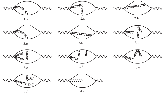
Figure 1: Feynman diagrams for the $\bar{q}q$-hybrid mixed state.

Collecting all the contributions to the correlator $\Pi_{\bar{q}Gq\bar{q}q}$ from Figure 1, we obtain

$$\Pi_{\bar{q}Gq\bar{q}q}(q^{2})= -\frac{2}{9\pi^{2}}\frac{\alpha_{s}}{\pi}q^{2}\left[\log\left(\frac{-q^{2}}{\nu^{2}}\right)-\frac{3}{2}\right]$$ (16)

$$+\frac{8}{9}\frac{\alpha_{s}}{\pi}\frac{1}{q^{2}}\left[\log\left(\frac{-q^{2}}{\nu^{2}}\right)-\frac{49}{6}\right]\left\langle m\bar{q}q\right\rangle$$

$$-\frac{2}{3}\frac{\alpha_{s}}{\pi}\frac{1}{q^{2}}\left\langle G^{2}\right\rangle-\frac{16}{9}\frac{g^{2}}{q^{4}}\left\langle\bar{q}q\right\rangle^{2}+\frac{1}{72}\frac{g^{3}}{\pi^{2}}\frac{1}{q^{4}}\left\langle G^{3}\right\rangle+\frac{8}{3}\frac{g}{q^{4}}\left\langle m\bar{q}Gq\right\rangle\textrm{,}$$

where we use the BMHV scheme to calculate traces in $D$ dimension to keep anti-commutativity of $\gamma_{5}$ ref_article13 ; ref_article14 .

By using the 50%-10% method described above, we obtain the sum rules window for $\tau$ in the range of $(0.32\textrm{GeV}^{-2},0.62\textrm{GeV}^{-2})$ for the $1^{--}$ mixing correlator. Minimizing $\chi^{2}$ leads to the solution

$$\left\{s_{0},\left|\frac{f_{1}f^{*}_{2}+f^{*}_{1}f_{2}}{2}\right|,m_{\bar{q}Gq\bar{q}q}\right\}=\left\{3.12^{+0.15}_{-0.13}\textrm{GeV}^{2},0.0126^{+0.0006}_{-0.0006}\textrm{GeV}^{4},0.737^{+0.058}_{-0.050}\textrm{GeV}\right\}.$$ (17)

The decay constants of currents $j_{1\mu}$ and $j_{2\mu}$ with pure $1^{--}$ hybrid and $\bar{q}q$ states respectively are $f_{\bar{q}q}^{{}^{\prime}}=(0.770\textrm{GeV})\times(0.153\textrm{GeV})$ for the pure $1^{--}$ $\bar{q}q$ state, and $f_{\bar{q}Gq}^{{}^{\prime}}=(2.34^{3}\textrm{GeV}^{3})\times(0.024\textrm{GeV})$ for the pure $1^{--}$ hybrid state ref_article21 ; ref_article24 . We consistently absorb mass factors in the definition of decay constants as described in the previous section. The mixing strength can then be estimated by computing the value of $N$

$$N_{\bar{q}Gq\bar{q}q}=\frac{0.0126\textrm{GeV}^{4}\times m_{\textrm{mix}}^{2}}{0.118\textrm{GeV}^{2}\times 0.308\textrm{GeV}^{4}}=0.19\textrm{,}$$ (18)

where $m_{\text{mix}}$ is the mixed state mass, i.e., $m_{\textrm{mix}}=m_{\bar{q}Gq\bar{q}q}$. The result $N_{\bar{q}Gq\bar{q}q}$=0.19 shows that the mixing strength is not as weak as expected since the mass of mixed state 0.770 GeV is very close to the $\rho$ meson, which is usually considered a very pure $\bar{q}q$ state . Then $N_{\bar{q}Gq\bar{q}q}$=0.19 is the strength (relative to the pure hybrid meson) of the $\rho$ meson coupling to the hybrid current. This suggests that the $\rho$ meson contribution to the sum rules for the $1^{--}$ hybrid is negligible. From these results we find that the hybrid component of the $\rho(1450)$ and $\rho(1570)$ is a few percent. However, we do not exclude a tetraquark and $\bar{q}q$ mixed state in this paper, which is a very possible $1^{--}$ mixed state in the same mass range.

4 Scalar $\bar{q}q$ and glueball mixed state

In this section, we define

$$j_{3u}=\frac{1}{2}m_{q}(\bar{u}(x)u(x)+\bar{d}(x)d(x))\textrm{,}$$ (19)

$$j_{3s}=m_{s}\bar{s}(x)s(x),$$

$$j_{4}=2\textrm{Tr}[\alpha_{s}G_{\mu\nu}(0)G_{\mu\nu}(0)],$$

where $m_{q}$=$(m_{u}+m_{d})/2$, to study the mixing between $0^{++}$ quark-antiquark state ($\bar{u}u+\bar{d}d$ or $\bar{s}s$) and glueball state.

Obviously chiral symmetry is broken if the off-diagonal mixing correlator

$$\Pi(q^{2})=i\int d^{4}x\,e^{iq\cdot x}\left\langle 0\left|j_{3u/3s}\left(x\right)j^{+}_{4}\left(0\right)\right|0\right\rangle$$ (20)

is non-zero, thus the perturbative contribution to the correlator must be proportional to the quark mass. As in Ref. Harnett:2008cw , we note that the effect of the renormalization of the glueball current $j_{4}$ involving operator mixing must be included ref_article12 , i.e., we should use the renormalized form of the glueball current

$$\left[G_{\mu\nu}^{a}G_{\mu\nu}^{a}\right]=\left(1-\frac{9}{2}\frac{\alpha_{s}}{\pi}\frac{1}{\epsilon}\right)G_{\mu\nu}^{aB}G_{\mu\nu}^{aB}+8\frac{\alpha_{s}}{\pi}\frac{1}{\epsilon}m^{B}\bar{q}^{B}q^{B}$$ (21)

in our calculation, where the upper script $B$ denotes bare quantities, and we set $D=4-\epsilon$ in the $\overline{\textrm{MS}}$ scheme. As note in Harnett:2008cw , the operator-mixing part of (21) will cancel $\log(-q^{2})/\epsilon$ divergence in the off-diagonal mixing correlator and keep the imaginary part of the correlator finite. The following gluon propagator has been used in our calculation ref_article11

$$\int dx\,e^{iq\cdot x}D^{ab}_{\mu\nu}\left(x,y\right)=-\frac{g_{\mu\nu}}{q^{2}}e^{iqy}\delta_{ab}+\frac{2g}{q^{4}}G_{\mu\nu}^{ab}\left(0\right)e^{iqy}-giy_{\varphi}G_{\varphi\rho}^{ab}\left(0\right)\frac{q_{\rho}}{q^{4}}e^{iqy}g_{\mu\nu}\textrm{,}$$ (22)

where $G_{\mu\nu}^{ab}=f^{abc}G_{\mu\nu}^{c}$.

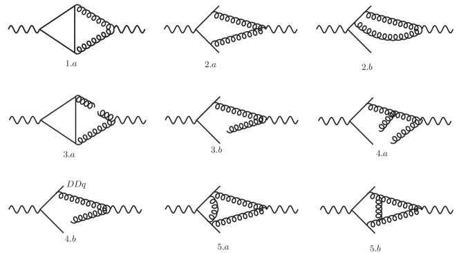
Figure 2: Feynman diagrams for the $\bar{q}q$-glueball mixed state. We omit most of the radiative correction diagrams which have been computed, and just list two of them at the end of the diagram terms. Note that 4.b just lists one expansion form.

The OPE result for the $\bar{q}q$-glueball mixed correlator from Figure 2 is

$$\Pi_{\bar{q}qGG}(q^{2})= -m^{2}q^{2}\log\left(-\frac{q^{2}}{\nu^{2}}\right)\left[-\frac{23}{2\pi}\left(\frac{\alpha_{s}}{\pi}\right)^{2}+\frac{3}{2\pi}\left(\frac{\alpha_{s}}{\pi}\right)^{2}\log\left(-\frac{q^{2}}{\nu^{2}}\right)\right]$$ (23)

$$+\left[-8\pi\left(\frac{\alpha_{s}}{\pi}\right)^{2}+18\pi\left(\frac{\alpha_{s}}{\pi}\right)^{3}\log\left(-\frac{q^{2}}{\nu^{2}}\right)-\frac{326}{3}\pi\left(\frac{\alpha_{s}}{\pi}\right)^{3}\right]\log\left(-\frac{q^{2}}{\nu^{2}}\right)\left\langle m\bar{q}q\right\rangle$$

$$-\frac{m^{2}}{q^{2}}\left[6\frac{\alpha_{s}}{\pi}-2\frac{\alpha_{s}}{\pi}\log\left(-\frac{q^{2}}{\nu^{2}}\right)\right]\left\langle\alpha_{s}G^{2}\right\rangle-4\frac{\alpha_{s}}{q^{2}}\left\langle gm\bar{q}Gq\right\rangle$$

$$+3\frac{\alpha_{s}}{\pi}\frac{A}{q^{4}}\left\langle gm\bar{q}Gq\right\rangle+\frac{4}{3}\frac{\alpha_{s}\pi}{q^{4}}\left\langle m\bar{q}q\right\rangle\left\langle\alpha_{s}G^{2}\right\rangle\textrm{,}$$

where 8 dimension operators are factorized in order to conduct a QCDSR analysis

$$\left\langle m\bar{q}G_{\mu\nu}G_{\mu\nu}q\right\rangle=\left\langle m\bar{q}q\right\rangle\left\langle G^{2}\right\rangle\textrm{,}$$ (24)

$$\left\langle m\bar{q}\left[G_{\mu\lambda},G_{\nu\lambda}\right]\sigma_{\mu\nu}q\right\rangle=A\left\langle m\bar{q}Gq\right\rangle\textrm{,}$$

with $A=\frac{g^{3}\left\langle G^{3}\right\rangle}{\alpha_{s}\left\langle G^{2}\right\rangle}$. In Eq. (23), $\bar{q}q$=$\frac{1}{2}(\bar{u}u+\bar{d}d)$, $m=m_{q}$ for $u,d$ quark case and $\bar{q}q$=$\bar{s}s$, $m=m_{s}$ for $s$ quark case. Our calculation confirms the perturbative, gluon condensate, mixed condensate, and leading-order quark condensate of Ref. Harnett:2008cw and extends the results for the correlator to include higher-dimension condensates and next-to-leading order quark condensate terms. We do not compute the radiative correction to the perturbative contribution because it is chirally suppressed and numerically small compared with the $\left\langle m\bar{q}q\right\rangle$ condensate.

The sum rule window, $\tau\in$ ( 0.03 GeV^-2, 0.25 GeV^-2) for the $u,d$ quark case, and $\tau\in$ ( 0.08 GeV^-2, 0.17 GeV^-2) for the $s$ quark case are obtained by demanding that 8D contributions are 1/4 of the 6D, thus 8D contributions is less than 5% of $R^{\textrm{(OPE)}}(\tau)$. With the presence of more terms in the OPE for the glueball mixing correlator, we are able to extend the criterion used for the hybrid to encompass OPE convergence from higher-dimension condensates. Ratios of different dimensional OPE contributions are shown in Figs. 3 and 4.

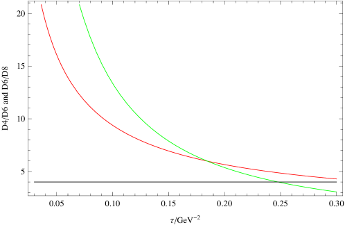
Figure 3: Ratios of different dimension contributions to the OPE are shown as a function of $\tau$ for the $u,d$ quark case. The red curve represents the 4D/6D ratio and the green line corresponds to 6D/8D.

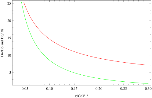
Figure 4: Ratios of different dimension contributions to the OPE are shown as a function of $\tau$ for the $s$ quark case. The red curve represents the 4D/6D ratio and the green line corresponds to 6D/8D.

The solutions that minimize $\chi^{2}$ are

$$\left\{s_{0},\left|\frac{f_{3u}f^{*}_{G}+f^{*}_{3u}f_{G}}{2}\right|,m_{\bar{u}uGG}\right\}=\left\{18.13^{+0.42}_{-0.42}\textrm{GeV}^{2},0.000291^{+0.000032}_{-0.000029}\textrm{GeV}^{6},0.867^{+0.052}_{-0.066}\textrm{GeV}\right\}\textrm{,}$$ (25)

$$\left\{s_{0},\left|\frac{f_{3s}f^{*}_{G}+f^{*}_{3s}f_{G}}{2}\right|,m_{\bar{s}sGG}\right\}=\left\{15.21^{+0.26}_{-0.28}\textrm{GeV}^{2},0.0158^{+0.0027}_{-0.0022}\textrm{GeV}^{6},1.654^{+0.076}_{-0.085}\textrm{GeV}\right\}\textrm{,}$$

where the first line is solution for $u,d$ quark case, and the second line is solution for $s$ quark case. The result (25) suggests that $f_{0}(500)$ and $f_{0}(1710)$ are respectively good candidates for mixed states of glueballs with $\bar{q}q$ and $\bar{s}s$ components. The $f_{0}(980)$ may also couple to $\bar{q}q$, but its coupling should be much weaker than the $f_{0}(500)$ ref_article27 . There is excellent agreement between the $\bar{q}q$ mass prediction (25) and that of Ref. Harnett:2008cw . Taking into account the differences from Ref. Harnett:2008cw in the field-theoretical content (e.g., higher-dimension condensates) and the use of Laplace versus Gaussian sum-rules that weight the OPE terms in fundamentally different ways, the agreement is remarkable. The $\bar{s}s$ case was not studied in Ref. Harnett:2008cw so no comparison with previous work is possible.

Finally, we estimate the mixing strength of these two states with same method we have used in the $1^{--}$ case. The relevant decay constants for the pure $0^{++}$ $\bar{q}q$ state and glueball have been obtained in literature: $f^{{}^{\prime}}_{q}$=0.5GeV$\times$0.64GeV for $\frac{1}{\sqrt{2}}(\bar{u}u+\bar{d}d)$, $f^{{}^{\prime}}_{s}$=0.98GeV$\times$0.41GeV for $\bar{s}s$, $f^{{}^{\prime}}_{G}$=$1.53^{2}$GeV²$\times$1.01GeV for glueball ref_article27 ; ref_article28 ; ref_article29 . Collecting all the parameters we compute $N_{\bar{u}uGG/\bar{s}sGG}$

$$N_{\bar{u}uGG}=\frac{0.000291\textrm{GeV}^{6}}{0.32\textrm{GeV}^{2}\times 2.36\textrm{GeV}^{3}\times m_{q}}=0.11\textrm{,}$$ (26)

$$N_{\bar{s}sGG}=\frac{0.0158\textrm{GeV}^{6}}{0.40\textrm{GeV}^{2}\times 2.36\textrm{GeV}^{3}\times m_{s}}=0.17\textrm{,}$$

where we have used masses of $u$, $d$ and $s$ quarks at the energy scale $\mu_{0}$=2 GeVref_article1 , which corresponds to the energy scale at which decay constants were derived in ref_article27 (since $m_{q}f^{{}^{\prime}}_{q}$ and $m_{s}f^{{}^{\prime}}_{s}$ are energy scale independent), i.e.,

$$m_{q}=\left(m_{u}+m_{d}\right)/2=3.5~{}\textrm{MeV},~{}m_{s}=96~{}\textrm{MeV}.$$ (27)

We divide by the quark mass in the above calculation because of different $\bar{q}q$ current definitions.

Comparing to $N$ in $1^{--}$, we see that the mixing strength of these two states are smaller but close to the $1^{--}$ case. It shows that these states are weakly coupled with one of two currents. This result should not be surprising because the mixing is chirally suppressed in the perturbative corrections. The mixing is dominated by non-perturbative chiral-violating condensate contributions, which converge slowly. In order to make the OPE series convergent, we have to use a window with a large energy scale where the low-energy condensate terms are suppressed. The coupling we obtain is therefore referenced to an energy scale far from the mass of the state, so our conclusion may change when the energy scale is decreased to the resonance mass. Furthermore, there is a large mass difference between $f_{0}(500)$ and $f_{0}(1710)$, which cannot be explained by the difference in the quark masses and condensates, so we suggest that, for the relative mixture of $\bar{q}q$ and gluonic content, the $f_{0}(500)$ is dominated by a $\bar{u}u+\bar{d}d$ component and $f_{0}(1710)$ is dominated by a glueball component. It is important to emphasize that the off-diagonal correlator (20) explores the mixing of gluonic and $\bar{q}q$ components, so our analysis does not constrain tetraquark components of the $f_{0}$ states.

A meaningful comparison with the mixing results of Ref. Harnett:2008cw is difficult because different aspects were explored. In Harnett:2008cw , the Gaussian sum-rule permitted study of multiple states in the off-diagonal correlator, and a strong mixing between these states was found, but no analysis of pure states was performed to allow comparison with the mixing parameter $N$. Nevertheless, Ref. Harnett:2008cw does also conclude that an approximately $1.5\,{\rm GeV}$ state is predominantly a glueball.

Because of the proximity in mass, it is easy to understand that there is a stronger mixing between $\bar{s}s$ and glueball than $\bar{u}u+\bar{d}d$ and glueball, however, it is subtle why the sum rules select a heavier glueball mixing with a few percent of $\bar{s}s$ rather than a lighter $\bar{s}s$ with a few percent of glueball. The only reason emerging from the sum rules is that the couplings of $\bar{s}s$ state to the currents (19) is not as strong as those of the glueball state.

In principle, it is possible that there is more than one state giving comparable contributions to the correlator (even though the simulation shows single pole model works well), then the average mass of these contributing states should be between 600 MeV and 1700 MeV (i.e., the range of the low lying $0^{++}$ states found in experiments). We could use the mass prediction in Eq. (25) to estimate the mixing information. In the $u,d$ quark case, the average mass is 867 MeV. This excludes the case that heavier states have a large contribution to the mixing. In the $s$ quark case, the result also prohibits a large contribution from the states much lighter than 1600 MeV.

Superficially one might expect a large sensitivity to the quark mass parameters because the perturbative process in the mixing correlator are proportional to the square of the quark mass. However, the constraints on the sum-rule working window of $\tau$ limit the sensitivity to these perturbative corrections. As the lower limit on $\tau$ is decreased, the single pole model will begin to fail (i.e., the excited states and continuum will give a large contribution) while the perturbative contributions for non-strange quarks remains small. As the upper limit on $\tau$ is increased to $\tau=0.3~{}\textrm{GeV}^{2}$ OPE convergence begins to fail. Thus for any reasonable variation in the working window in $\tau$ we still find that non-perturbative contributions will dominate the mixing.

5 Summary

In this paper we have used QCD sum-rule methods for off-diagonal correlation functions to study the mixing of $\bar{q}q$ with hybrid and glueball components for the $1^{--}$ vector and $0^{++}$ scalar channels. The mass prediction for the $1^{--}$ mixed state is $0.737^{+0.058}_{-0.050}$ GeV, consistent with the mass of $\rho$(770) within the errors and very close to the mass obtained in QCDSR using solely the vector interpolating current $\bar{q}\gamma_{\mu}q$ ref_article24 . This result disfavours a large mixing between $1^{--}$ light $\bar{q}q$ and hybrid mesons.

For $0^{++}$ particles, we find the mass predictions are respectively $0.867^{+0.052}_{-0.066}$ GeV for the $\bar{u}u+\bar{d}d$-$GG$ mixed state and $1.654^{+0.076}_{-0.085}$ GeV for the $\bar{s}s$-$GG$ mixed state. These results qualitatively show that $f_{0}(500)$ and $f_{0}(1710)$ can be candidates in these two cases. We have estimated the “mixing strength” defined in (11) for these states which represents whether the $\bar{q}q$ and gluonic components of the “physical state” under consideration is more of a mixed state or a pure state. From the mixing strength one can see that the $\bar{q}q$ and gluonic components of these scalar states are likely not to be strongly mixed, with the $f_{0}(1710)$ being close to a pure glueball. In fact, $\rho$(770) is generally considered as a very pure state (which can also be seen from our previous analysis). If we set the $\rho$ meson as a standard to examine other states, we see that $f_{0}(500)$ is even more pure than $\rho$(770), while $f_{0}(1710)$, which was considered as a strongly mixed state of a $\bar{q}q$ meson and a glueball, has a similar mixing strength as $\rho$(770).

As noted earlier, our analysis through the off-diagonal correlator (20) examines the mixing of the $\bar{q}q$ and gluonic components, so our results do not constrain the four-quark content of the $f_{0}(500)$. However, we can conclude that the $f_{0}(500)$ has both gluonic and $\bar{q}q$ components because this state emerges from the mixed correlator (20), and our small-mixing result suggests that the relative proportion of one of component may dominate the other. In some previous analyses the relative proportion of gluonic components are more prominent than $\bar{q}q$ (see e.g., Narison:1996fm ; Narison:2005wc ; Ochs:2013gi ; Mennessier:2010xg ; Minkowski:1998mf ) , while in other approaches it is the opposite (see e.g., 06_F ; Albaladejo:2008qa ).

Finally, it should be noted that the accuracy of our work is subject to some factors. For the $0^{++}$ case, we are constrained to do our analysis in a window with a relatively large Borel scale $\frac{1}{\tau}$ (compared to the resonance mass) to ensure OPE convergence, which however may also suppress the non-perturbative QCD effects that dominate the mixing. Furthermore, our analysis is also sensitive to the decay constants of the pure states (such as the $1^{--}$ hybrid and the $0^{++}$ glueball) which have not been measured in experiments and thus rely on sum rule determinations and model calculations that may have input parameters in tension with our work.

Clearly it is complicated to rigorously consider the mixing in QCD, and our sum rule analysis provides estimates which suggest the effects of the mixing between hybrids/glueballs and ordinary $\bar{q}q$ mesons are very limited in the vector and scalar channels. The methods of this work can be extended to the mixing between tetraquarks and hybrids or $\bar{q}q$ states. It would be of particular interest if such mixing is not be suppressed in the sum-rule working interval by some (approximate) symmetries such as the chiral symmetry.

Appendix A QCDSR fitting results

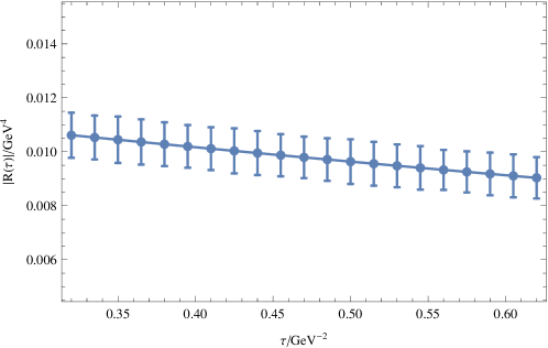
Figure 5: QCDSR minimum-$\chi^{2}$ fit for the $\bar{q}q$-hybrid mixed state: the dots represent the QCD side of the master equation (9), and the middle line represents phenomenological side of (9). The error bars are induced by 10% uncertainty of the phenomenological parameters of Table 1.

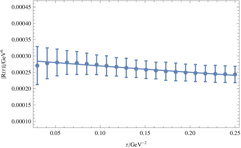
Figure 6: QCDSR minimum-$\chi^{2}$ fit for the $\bar{u}u$+$\bar{d}d$ and glueball mixed state: the dots represent QCD side of the master equation (9), and the middle line represents phenomenological side of (9). The error bars are induced by 10% uncertainty of the phenomenological parameters in of the phenomenological parameters of Table 1.

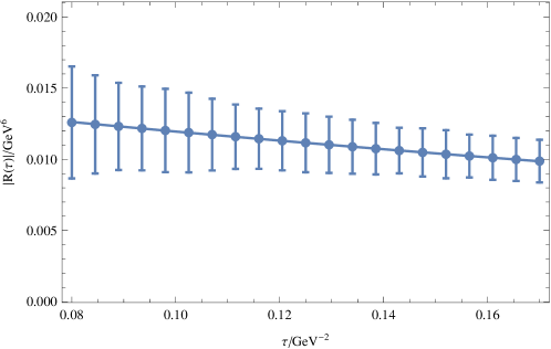
Figure 7: QCDSR minimum-$\chi^{2}$ fit for the $ss$ and glueball mixed state: the dots represent QCD side of the master equation (9), and the middle line represents phenomenological side of (9). The error bars are induced by 10% uncertainty of the phenomenological parameters in of the phenomenological parameters of Table 1

References

- (1) M. Tanabashi et al. [Particle Data Group], Review of Particle Physics, Phys. Rev. D 98 (2018) 030001.
- (2) M. S. Chanowitz and S. R. Sharpe, Hybrids: Mixed States of Quarks and Gluons, Nucl. Phys. B 222 (1983) 221.
- (3) Y. R. Liu, H. X. Chen, W. Chen, X. Liu and S. L. Zhu, Pentaquark and Tetraquark states, Prog. Part. Nucl. Phys. 107 (2019) 237.
- (4) H. X. Chen, W. Chen, X. Liu and S. L. Zhu, The hidden-charm pentaquark and tetraquark states, Phys. Rept. 639 (2016) 1.
- (5) J. Govaerts, F. de Viron, D. Gusbin and J. Weyers, Exotic mesons from QCD sum rules, Phys. Lett. B 128 (1983) 262.
- (6) J. Govaerts, F. de Viron, D. Gusbin and J. Weyers, QCD Sum Rules and Hybrid Mesons, Nucl. Phys. B 248 (1984) 1.
- (7) M. A. Shifman, A. I. Vainshtein and V. I. Zakharov, QCD and Resonance Physics. Theoretical Foundations, Nucl. Phys. B 147 (1979) 385.
- (8) R. M. Albuquerque, F. Fanomezana, S. Narison and A. Rabemananjara, and heavy four-quark and molecule states in QCD, Nucl.Phys.Proc.Suppl. 234 (2013) 158-161.
- (9) R. D. Matheus, S. Narison, M. Nielsen and J. M. Richard, “Can the X(3872) be a 1++ four-quark state?, Phys. Rev. D 75 (2007) 014005
- (10) H. Y. Jin and J. G. Korner, Radiative corrections to the correlator of light hybrid currents,, Phys. Rev. D 64 (2001) 074002.
- (11) H. Y. Jin, J. G. Korner and T. G. Steele, Improved determination of the mass of the light hybrid meson from QCD sum rules, Phys. Rev. D 67 (2003) 014025.
- (12) S. Narison, light exotic mesons in QCD, Phys. Lett. B 675 (2009) 319.
- (13) J. Ho, R. Berg, T. G. Steele, W. Chen and D. Harnett, Mass Calculations of Light Quarkonium, Exotic Hybrid Mesons from Gaussian Sum-Rules, Phys. Rev. D 98 (2018) 096020.
- (14) Z. R. Huang, H. Y. Jin and Z. F. Zhang, New predictions on the mass of the light hybrid meson from QCD sum rules, JHEP, 1504 (2015) 004.
- (15) Z. R. Huang, H. Y. Jin, T. G. Steele and Z. F. Zhang, Revisiting the b and decay modes of the 1-+ light hybrid state with light-cone QCD sum rules, Phys. Rev. D 94 (2016) 054037.
- (16) Z. R. Huang, W. Chen, T. G. Steele, Z. F. Zhang and H. Y. Jin, Investigation of the light four-quark states with exotic , Phys. Rev. D 95 (2017) 076017.
- (17) Y. C. Fu, Z. R. Huang, Z. F. Zhang and W. Chen, Exotic tetraquark states with , Phys. Rev. D 99 (2019), 014025.
- (18) Z. f. Zhang and H. y. Jin, Instanton Effects in QCD Sum Rules for the Hybrid, Phys. Rev. D 85 (2012) 054007.
- (19) W. Chen, R. T. Kleiv, T. G. Steele, B. Bulthuis, D. Harnett, J. Ho, T. Richards and S. L. Zhu, Mass Spectrum of Heavy Quarkonium Hybrids, JHEP 1309 (2013) 019.
- (20) W. Chen, H. y. Jin, R. T. Kleiv, T. G. Steele, M. Wang and Q. Xu, QCD sum-rule interpretation of X(3872) with mixtures of hybrid charmonium and molecular currents, Phys. Rev. D 88 (2013) 045027.
- (21) C. K. Jiao, W. Chen, H. X. Chen and S. L. Zhu, The Possible J**PC = 0– Exotic State, Phys. Rev. D 79 (2009) 114034
- (22) H. X. Chen, A. Hosaka and S. L. Zhu, The I**G J**PC = 1- 1-+ Tetraquark States, Phys. Rev. D 78 (2008) 054017.
- (23) R. M. Albuquerque, M. E. Bracco and M. Nielsen, A QCD sum rule calculation for the Y(4140) narrow structure, Phys. Lett. B 678 (2009) 186.
- (24) J. R. Zhang, M. Zhong and M. Q. Huang, Could be a molecular state?, Phys. Lett. B 704 (2011) 312
- (25) A. Pimikov, H. J. Lee, N. Kochelev, P. Zhang and V. Khandramai, Exotic glueball states in QCD sum rules, Phys. Rev. D 96 (2017) 114024.
- (26) L. Tang and C. F. Qiao, Mass spectra of , , and exotic glueballs, Nucl. Phys. B 904 (2016) 282.
- (27) D. Harnett, R. T. Kleiv, K. Moats and T. G. Steele, Near-Maximal Mixing of Scalar Gluonium and Quark Mesons: A Gaussian Sum-Rule Analysis, Nucl. Phys. A 850 (2011) 110.
- (28) D. Harnett and T. G. Steele, A Gaussian sum rules analysis of scalar glueballs, Nucl. Phys. A 695 (2001) 205.
- (29) J. Ho, D. Harnett and T. G. Steele, Masses of Open-Flavour Heavy-Light Hybrids from QCD Sum-Rules, JHEP 1705 (2017) 149.
- (30) W. Chen, T. G. Steele and S. L. Zhu, Heavy tetraquark states and quarkonium hybrids, The Universe 2 (2014) 13.
- (31) S. Narison, Masses, decays and mixings of gluonia in QCD, Nucl. Phys. B 509 (1998) 312.
- (32) S. Narison, QCD tests of the puzzling scalar mesons, Phys. Rev. D 73 (2006) 114024.
- (33) C. Amsler and F. E. Close, Evidence for a a scalar glueball, Phys. Lett. B 353 (1995) 385.
- (34) C. Amsler and F. E. Close, Is a scalar glueball? Phys. Rev. D 53 (1996) 295.
- (35) S. Narison, N. Pak and N. Paver, Meson - Gluonium Mixing From QCD Sum Rules, Phys. Lett. 147B (1984) 162.
- (36) A. Palameta, D. Harnett and T. G. Steele, Meson-Hybrid Mixing in Heavy Quarkonium from QCD Sum-Rules, Phys. Rev. D 98 (2018) 074014.
- (37) A. Palameta, J. Ho, D. Harnett and T. G. Steele, QCD sum-rules analysis of vector () heavy quarkonium meson-hybrid mixing, Phys. Rev. D 97 (2018) 034001.
- (38) T. Barnes, F. E. Close, F. de Viron and J. Weyers, Q anti-Q G Hermaphrodite Mesons in the MIT Bag Model, Nucl. Phys. B 224 (1983) 241.
- (39) C. J. Morningstar and M. J. Peardon, The Glueball spectrum from an anisotropic lattice study, Phys. Rev. D 60 (1999) 034509; Y. Chen et al., Glueball spectrum and matrix elements on anisotropic lattices, Phys. Rev. D 73 (1999) 034509.
- (40) L. Y. Dai, J. Fuentes-Martín and J. Portolés, Scalar-involved three-point Green functions and their phenomenology, Phys. Rev. D 99 (2019) 114015.
- (41) D. Black, A.H. Fariborz and J. Schechter, Mechanism for a next-to-lowest lying scalar meson nonet, Phys. Rev. D 61 (2000) 074001.
- (42) F. Close and N. Tornqvist, Scalar mesons above and below 1-GeV, J. Phys. G 28 (2002) 249.
- (43) T. Teshima, I. Kitamura and N. Morisita, Mixing among light scalar mesons and L=1 q anti-q scalar mesons, J. Phys. G 28 (2002) 1391.
- (44) M. Napsuciale and S. Rodriguez, A Chiral model for anti-q q and anti-qq qq mesons, Phys. Rev. D 70 (2004) 094043 .
- (45) A.H. Fariborz, Mass Uncertainties of f0(600) and f0(1370) and their Effects on Determination of the Quark and Glueball Admixtures of the I=0 Scalar Mesons, Phys. Rev. D 74 (2006) 054030.
- (46) G. ’t Hooft, G. Isidori, L. Maiani, A.D. Polosa and V. Riquer, A Theory of Scalar Mesons, Phys. Lett. B 662 (2008) 424.
- (47) A.H. Fariborz, R. Jora and J. Schechter, Global aspects of the scalar meson puzzle, Phys. Rev. D 79(2009) 074014.
- (48) A.H. Fariborz, R. Jora and J. Schechter, Note on a sigma model connection with instanton dynamics, Phys. Rev. D 77 (2008) 094004.
- (49) A.H. Fariborz, R. Jora and J. Schechter, Toy model for two chiral nonets, Phys. Rev. D 72 (2005) 034001.
- (50) R.L. Jaffe, Multi-Quark Hadrons. 1. The Phenomenology of (2 Quark 2 anti-Quark) Mesons, Phys. Rev. D 15 (1977) 267.
- (51) A. l. Zhang, Four quark state in QCD, Phys. Rev. D 61 (2000) 114021.
- (52) T. V. Brito, F. S. Navarra, M. Nielsen and M. E. Bracco, QCD sum rule approach for the light scalar mesons as four-quark states, Phys. Lett. B 608 (2005) 69.
- (53) H. X. Chen, A. Hosaka and S. L. Zhu, Light Scalar Tetraquark Mesons in the QCD Sum Rule, Phys. Rev. D 76 (2007) 094025; H. X. Chen, A. Hosaka and S. L. Zhu, QCD sum rule study of the masses of light tetraquark scalar mesons, Phys. Lett. B 650 (2007) 369.
- (54) V. Elias, A. H. Fariborz, F. Shi and T. G. Steele, QCD sum rule consistency of lowest lying q anti-q scalar resonances, Nucl. Phys. A 633 (1998) 279.
- (55) Z. f. Zhang, H. y. Jin and T. G. Steele, Revisiting and light hybrids from Monte-Carlo based QCD sum rules, Chin. Phys. Lett. 31 (2014) 051201.
- (56) A. Hart et al. [UKQCD Collaboration], A Lattice study of the masses of singlet 0++ mesons, Phys. Rev. D 74 (2006) 114504.
- (57) M. A. Shifman, A. I. Vainshtein and V. I. Zakharov, QCD and Resonance Physics: Applications, Nucl. Phys. B 147 (1979) 448.
- (58) S. Aoki et al. [Flavour Lattice Averaging Group], FLAG Review 2019, arXiv:1902.08191.
- (59) S. Narison, Mini-review on QCD spectral sum rules, Nucl. Part. Phys. Proc. 258-259 (2015) 189.
- (60) V. A. Novikov, M. A. Shifman, A. I. Vainshtein and V. I. Zakharov,Are All Hadrons Alike? Nucl. Phys. B 191 (1981) 301.
- (61) S. Narison, Heavy quarkonia mass-splittings in QCD: test of the -expansion and estimates of and , Nucl. Phys. Proc. Suppl. 54A (1997) 238.
- (62) L. J. Reinders, H. Rubinstein and S. Yazaki, Hadron Properties from QCD Sum Rules, Phys. Rept. 127 (1985) 1.
- (63) A. G. Grozin, Methods of calculation of higher power corrections in QCD, Int. J. Mod. Phys. A 10 (1995) 3497.
- (64) G. ’t Hooft and M. J. G. Veltman, Regularization and Renormalization of Gauge Fields, Nucl. Phys. B 44 (1972) 189.
- (65) M. Pernici, Seminaive dimensional renormalization, Nucl. Phys. B 582 (2000) 733.
- (66) Q. N. Wang, Z. F. Zhang, T. G. Steele, H. Y. Jin and Z. R. Huang, A comprehensive revisit of the meson with improved Monte-Carlo based QCD sum rules, Chin. Phys. C, 41 (2017) 074107.
- (67) F. K. Guo, P. N. Shen, Z. G. Wang, W. H. Liang and L. S. Kisslinger, Light vector hybrid states via QCD sum rules, arXiv: 0703062 (2007).
- (68) R. Tarrach, The renormalization of FF, Nucl. Phys. B 196 (1982) 45.
- (69) V. A. Novikov, M. A. Shifman, A. I. Vainshtein and V. I. Zakharov, Calculations in external fields in quantum chromodynamics. Technical Review, Fortsch. Phys. 32 (1984) 585.
- (70) J. M. Yuan, Z. F. Zhang, T. G. Steele, H. Y. Jin and Z. R. Huang, Constraint on the light quark mass from QCD sum rules in the scalar channel, Phys. Rev. D 96 (2017) 014034.
- (71) H. Forkel, Direct instantons, topological charge screening and QCD glueball sum rules, Phys. Rev. D 71 (2005) 054008.
- (72) H. Forkel, Scalar gluonium and instantons, Phys. Rev. D 64 (2001) 034015.
- (73) W. Ochs, The Status of Glueballs, J. Phys. G 40 (2013) 043001.
- (74) G. Mennessier, S. Narison and X. G. Wang, The sigma and from scatterings data, Phys. Lett. B 688 (2010) 59.
- (75) P. Minkowski and W. Ochs, “Identification of the glueballs and the scalar meson nonet of lowest mass, Eur. Phys. J. C 9 (1999) 283.
- (76) M. Albaladejo and J. A. Oller, Identification of a Scalar Glueball, Phys. Rev. Lett. 101 (2008) 252002.