Subset Selection for Matrices with Fixed Blocks

Abstract.

Subset selection for matrices is the task of extracting a column sub-matrix from a given matrix $B\in\mathbb{R}^{n\times m}$ with $m>n$ such that the pseudoinverse of the sampled matrix has as small Frobenius or spectral norm as possible. In this paper, we consider a more general problem of subset selection for matrices that allows a block to be fixed at the beginning. Under this setting, we provide a deterministic method for selecting a column sub-matrix from $B$. We also present a bound for both the Frobenius and spectral norms of the pseudoinverse of the sampled matrix, showing that the bound is asymptotically optimal. The main technology for proving this result is the interlacing families of polynomials developed by Marcus, Spielman, and Srivastava. This idea also results in a deterministic greedy selection algorithm that produces the sub-matrix promised by our result.

1. Introduction

1.1. Subset selection for matrices

Subset selection for matrices aims to select a column sub-matrix from a given matrix $B\in\mathbb{R}^{n\times m}$ with $m>n$ such that the sampled matrix is well-conditioned. For convenience, we assume that $B$ is full-rank, i.e., $\mbox{rank}(B)=n$. Given ${\mathcal{S}}\subseteq[m]:=\{1,\ldots,m\}$, the cardinality of the set ${\mathcal{S}}$ is denoted by $|{\mathcal{S}}|$. We use $B_{{\mathcal{S}}}$ to denote the sub-matrix of $B$ obtained by extracting the columns of $B$ indexed by ${\mathcal{S}}$ and use $B_{\mathcal{S}}^{\dagger}$ to denote the Moore-Penrose pseudoinverse of $B_{{\mathcal{S}}}$. We use $\|B\|_{2}:=\max\limits_{\|x\|_{2}=1}\|Bx\|_{2}$ and $\|B\|_{F}:=\sqrt{\mbox{Tr}(BB^{T})}$ to denote, respectively, the spectral norm and Frobenius norm of $B$. Let $k\in[n,m-1]:=\{n,\ldots,m-1\}$ be a sampling parameter. We can formulate the subset selection for matrices as follows.

Problem 1.1.

Find a subset ${\mathcal{S}}_{opt}\subset\{1,2,\ldots,m\}$ with cardinality at most $k$ such that $\mbox{rank}(B_{\mathcal{S}_{opt}})=\mbox{rank}(B)$ and $\|B_{\mathcal{S}_{opt}}^{\dagger}\|_{\xi}^{2}$ is minimized, i.e.,

$$\mathcal{S}_{opt}\in\mathop{\rm argmin}\limits_{\mathcal{S}\in\mathcal{F}(B,k)}\|B_{\mathcal{S}}^{\dagger}\|_{\xi}^{2},$$

where $\mathcal{F}(B,k)=\{\mathcal{S}:|\mathcal{S}|\leq k,\mbox{rank}(B_{\mathcal{S}})=\mbox{rank}(B)\}$ and $\xi=2$ and F denotes the spectral and Frobenius matrix norm, respectively.

Problem 1.1 is raised in many applied areas, such as preconditioning for solving linear systems[1], sensor selection [15], graph signal processing [9, 30], and feature selection in $k$-means clustering [7, 8]. In [2], Avron and Boutsidis showed an interesting connection between Problem 1.1 and the combinatorial problem of finding a low-stretch spanning tree in an undirected graph. In the statistics literature, the subset selection problem has also been studied. For instance, the solution to Problem 1.1 has statistically optimal design for linear regression provided $\xi=F$ [12, 24].

One simple method for solving Problem 1.1 is to evaluate the performance of all ${m\choose k}$ possible subsets with size $k$, but evidently it is computationally expensive unless $m$ or $k$ is very small. In [11], Çivril and Magdon-Ismail studied the complexity of the spectral norm version of Problem 1.1, where they showed that it is NP-hard. Several heuristics have been proposed to approximately solve the subset selection problem (see Section 1.3).

1.2. Our contribution

In this paper, we consider a generalized version of subset selection for matrices, where we have a matrix $A$ fixed at first, and our goal is to supplement this matrix by adding columns of $B$ such that $[A\ B_{\mathcal{S}}]$ has as small Frobenius or spectral norm as possible. Usually, $A$ is chosen as a column sub-matrix of $B$. This notion of keeping a fixed block of $B$ is useful if we already know that such a block has some distinguished properties. We state the problem as follows:

Problem 1.2.

Suppose that $A\in\mathbb{R}^{n\times\ell}$ and $B\in\mathbb{R}^{n\times m}$ with $\mbox{rank}(A)=r$ and $rank\big{(}[A\ B]\big{)}=n$. Find a subset ${\mathcal{S}}_{opt}\subset\{1,2,\ldots,m\}$ with cardinality at most $k\in[n-r,m-1]$ such that $\mbox{rank}([A\ B_{\mathcal{S}_{opt}}])=\mbox{rank}([A\ B])$ and $\|[A\ B_{\mathcal{S}_{opt}}]^{\dagger}\|_{\xi}^{2}$ is minimized, i.e.,

$$\mathcal{S}_{opt}\in\mathop{\rm argmin}\limits_{\mathcal{S}\in\mathcal{F}(B,k)}\big{\|}([A\ B_{\mathcal{S}}])^{\dagger}\big{\|}_{\xi}^{2},$$

where $\mathcal{F}(B,k)=\{\mathcal{S}:|\mathcal{S}|\leq k,\mbox{rank}([A\ B_{\mathcal{S}}])=\mbox{rank}([A\ B])\}$ and $\xi=2$ and F denotes the spectral and Frobenius matrix norm, respectively.

We would like to mention that the Frobenius norm version of Problem 1.2 was considered in [29]. If we take $A=0$, then Problem 1.2 is reduced to Problem 1.1. Hence, the results presented in this paper also present a solution to Problem 1.1. We next state the main result of this paper. For convenience, throughout this paper, we set

(1) $$\Gamma(m,n,k,r):=\frac{m^{2}}{\big{(}\sqrt{(k+1)(m-n+r)}-\sqrt{(n-r)(m-k-1)}\big{)}^{2}},$$

where $m,n,k,r\in{\mathbb{Z}}$. We have the following result for Problem 1.2.

Theorem 1.3.

Suppose that $A\in\mathbb{R}^{n\times\ell}$ and $B\in\mathbb{R}^{n\times m}$ with $\mbox{rank}(A)=r$ and $rank\big{(}[A\ B]\big{)}=n$. Then for any fixed $k\in[n-r,m-1]$, there exists a subset $\mathcal{S}_{0}\subseteq[m]$ with cardinality $k$ such that $[A\ B_{\mathcal{S}_{0}}]$ is full-rank and

(2) $$\big{\|}\big{(}[A\ B_{\mathcal{S}_{0}}]\big{)}^{\dagger}\big{\|}_{\xi}^{2}\leq\Gamma(m,n,k,r)\cdot\bigg{(}1+\frac{\|A^{\dagger}B\|^{2}_{F}}{m-n+r}\bigg{)}\cdot\big{\|}([A\ \,B])^{\dagger}\big{\|}_{\xi}^{2},$$

where $\xi\in\{2,F\}$.

The proof of Theorem 1.3 provides a deterministic algorithm for computing the subset $\mathcal{S}_{0}$ in time $O(k(m-\frac{k}{2})n^{\theta}\log(1/\epsilon))$, where $\theta>2$ is the exponent of the complexity of matrix multiplication, which we will introduce it in Section 4.

Taking $A=0$ in Theorem 1.3, we obtain the following corollary.

Corollary 1.4.

Suppose that $B\in\mathbb{R}^{n\times m}$ with $rank\big{(}B\big{)}=n$. Then for any fixed $k\in[n,m-1]$, there exists a subset $\mathcal{S}_{0}\subseteq[m]$ with cardinality $k$ such that $rank(B_{\mathcal{S}_{0}})=n$ and for both $\xi=2$ and $F$,

(3) $$\big{\|}B_{\mathcal{S}_{0}}^{\dagger}\big{\|}_{\xi}^{2}\leq\Gamma(m,n,k,0)\cdot\big{\|}B^{\dagger}\big{\|}_{\xi}^{2}.$$

1.3. Related work

In this subsection, we give a summary of known results on the subset selection problem and also provide comparisons between our results and those of previous studies.

1.3.1. Lower bounds

A lower bound is defined as a non-negative number $\gamma$ such that there exists a matrix $B\in\mathbb{R}^{n\times m}$ satisfying

$$\|B^{\dagger}_{{\mathcal{S}}}\|_{\xi}^{2}\geq\gamma\|B^{\dagger}\|^{2}_{\xi}$$

for every ${\mathcal{S}}$ of cardinality $k\geq n$. Lower bounds for Problem 1.1 were studied in [2]. Particularly, for $\xi=2$, Theorem $4.3$ in [2] showed a lower bound is $\frac{m}{k}-1$. For $\xi=F$, according to Theorem $4.5$ in [2], we know a bound is $\frac{m}{k}-O(1)$ provided $k=O(n)$. The approximation bound presented in Corollary 1.4 asymptotically matches those bounds. Indeed, according to Corollary 1.4, we have

$$\|B_{\mathcal{S}}^{\dagger}\|_{\xi}^{2}\leq\Gamma(m,n,k,0)\cdot\|B^{\dagger}\|_{\xi}^{2}.$$

If $n/k$ is fixed, then $\Gamma(m,n,k,0)=O(m/k)$, which asymptotically matches the lower bounds presented in [2]. Besides, if $k/m$ is fixed and $m$ is large enough, then $\Gamma(m,n,k,0)\approx m/k$ which is close to the lower bound $m/k-1$.

1.3.2. Restricted invertibility principle

The restricted invertibility problem asks whether one can select a large number of linearly independent columns of $B$ and provide an estimation for the norm of the restricted inverse. To be more precise, one wants to find a subset ${\mathcal{S}}$, with cardinality $k\leq\mbox{rank}(B)$ being as large as possible, such that $\|B_{{\mathcal{S}}}x\|_{2}\geq c\|x\|_{2}$ for all $x\in\mathbb{R}^{|{\mathcal{S}}|}$ and to estimate the constant $c$. In [6], Bourgain and Tzafriri introduced the restricted invertibility problem and showed its applications in geometry and analysis. Later, their results were improved in [26, 27, 28, 25]. In [20], Marcus, Spielman, and Srivastava employed the method of interlacing families of polynomials to sharpen this result and presented a simple proof to the restricted invertibility principle. One can see [23] for a survey of the recent development in restricted invertibility.

Problem 1.1 is different from the restricted invertibility problem. In Problem 1.1, we require $|{\mathcal{S}}|\geq{\rm rank}(B)$, while in the restricted invertibility problem, one focuses on the case where $|{\mathcal{S}}|\leq{\rm rank}(B)$. We would like to mention that our proof for Theorem 1.3 is inspired by the method developed by Marcus, Spielman, and Srivastava [20] to study the restricted invertibility principle. We will introduce the main idea of the proof in Section 1.4.

1.3.3. Approximation bounds for $\xi=F$

We first focus on known bounds for

$$\|B_{\mathcal{S}}^{\dagger}\|_{F}^{2}/\|B^{\dagger}\|_{F}^{2}.$$

In [2, 13, 14], a greedy algorithm was developed, where one “bad” column of $B$ is removed at each step. As shown in [2, 13, 14], the greedy algorithm can find a subset ${\mathcal{S}}$ with $\lvert{\mathcal{S}}\rvert=k\geq n$ such that

(4) $$\|B_{\mathcal{S}}^{\dagger}\|_{F}^{2}\leq\frac{m-n+1}{k-n+1}\|B^{\dagger}\|_{F}^{2}$$

in $O(mn^{2}+mn(m-k))$ time. If $n/k<1$ is fixed, the bound $\frac{m-n+1}{k-n+1}$ in (4) is $O(m/k)$, which is as same as that in (3).

In [29], the Frobenius norm version of Problem 1.2 was studied. Let $A$ be a fixed matrix. The author of [29] showed that for any sampling parameter $k\in[n-\lfloor\|([A\ \,B])^{\dagger}A\|^{2}_{F}\rfloor,m-1]$, one can produce a subset ${\mathcal{S}}$ satisfying $\lvert{\mathcal{S}}\rvert=k$ in $O((n^{3}+mn^{2})(m-k))$ time while presenting an upper bound on $\big{\|}\big{(}[A\ B_{\mathcal{S}}]\big{)}^{\dagger}\big{\|}_{F}^{2}$. Note that Theorem 1.3 requires the sampling parameter $k\in[n-r,m-1]$, and hence it is available for a wider range of $k$. Here, we use the fact that $\|([A\ \,B])^{\dagger}A\|^{2}_{F}=\mbox{Tr}\big{(}(AA^{T}+BB^{T})^{-1}AA^{T}\big{)}\leq r$, and hence $n-r\leq n-\lfloor\|([A\ \,B])^{\dagger}A\|^{2}_{F}\rfloor$.

1.3.4. Approximation bounds for $\xi=2$

For $\xi=2$, an algorithm was developed in [2], which outputs ${\mathcal{S}}$ satisfying $\lvert{\mathcal{S}}\rvert=k$ and

(5) $$\|B_{\mathcal{S}}^{\dagger}\|_{2}^{2}\leq\left(1+\frac{n(m-k)}{k-n+1}\right)\|B^{\dagger}\|_{2}^{2}.$$

The algorithm runs in $O(mn^{2}+mn(m-k))$ time. If $n/k$ is fixed, the asymptotic bound in (5) is $O(m-k+1)$, which is larger than that in (3), i.e., $\Gamma(m,n,k,0)$. For $\xi=2$, to our knowledge, Problem 1.2 has not been considered in any previous papers, and Theorem 1.3 is the first work on an approximation bound as well as a deterministic algorithm for Problem 1.2.

1.3.5. Approximation bounds for both $\xi=2$ and $F$

In [2], a deterministic algorithm have developed for both $\xi=2$ and $F$. The algorithm, which runs in $O(kmn^{2})$ time, outputs a set ${\mathcal{S}}$ satisfying $\lvert\mathcal{S}\rvert=k>n$ and

(6) $$\|B_{\mathcal{S}}^{\dagger}\|_{\xi}^{2}\leq\left(1+\sqrt{\frac{m}{k}}\right)^{2}\left(1-\sqrt{\frac{n}{k}}\right)^{-2}\|B^{\dagger}\|_{\xi}^{2},\quad\xi\in\{2,F\}.$$

Noting that

$$\Gamma(m,n,k,0) \leq \bigg{(}1+\frac{\sqrt{n(k+1)}}{m}\bigg{)}^{-1}\frac{m}{(\sqrt{k+1}-\sqrt{n})^{2}}$$

$$< \frac{m}{(\sqrt{k+1}-\sqrt{n})^{2}}<\frac{(\sqrt{k}+\sqrt{m})^{2}}{(\sqrt{k}-\sqrt{n})^{2}}$$

$$= \bigg{(}1+\sqrt{\frac{m}{k}}\bigg{)}^{2}\bigg{(}1-\sqrt{\frac{n}{k}}\bigg{)}^{-2},$$

we obtain that

$$\Gamma(m,n,k,0)<\bigg{(}1+\sqrt{\frac{m}{k}}\bigg{)}^{2}\bigg{(}1-\sqrt{\frac{n}{k}}\bigg{)}^{-2}.$$

Hence the bound $\Gamma(m,n,k,0)$, which is presented in Corollary 1.4, is much better than the one in (6). Particularly, when $k$ tends to $n$, the approximation bound in (6) goes to infinity while $\Gamma(m,n,k,0)$ is still finite. Hence, the bound $\Gamma(m,n,k,0)$ is far better than the one in (6) when $k$ is close to $n$.

1.3.6. Algorithms

Many random algorithms have developed for solving Problem 1.1 (see [2]). In this paper, we focus on deterministic algorithms. Motivated by the proof of Theorem 1.3, we introduce a deterministic algorithm in Section 4, which outputs a subset ${\mathcal{S}}$ such that

$$\big{\|}\big{(}[A\ B_{\mathcal{S}}]\big{)}^{\dagger}\big{\|}_{\xi}^{2}\leq\Gamma(m,n,k,r)\cdot\bigg{(}1+\frac{\|A^{\dagger}B\|^{2}_{F}}{m-n+r}\bigg{)}\cdot\left(1+2k\epsilon\right)\cdot\big{\|}([A\ \,B])^{\dagger}\big{\|}_{\xi}^{2}$$

for any fixed $\epsilon\in(0,\frac{1}{2k})$. As shown in Theorem 4.1, the complexity of the algorithm is $O(k(m-\frac{k}{2})n^{\theta}\log(1/\epsilon))$ where $\theta>2$ is the exponent of matrix multiplication. We emphasize that our algorithm is faster than all algorithms mentioned in Section 1.3.3 and Section 1.3.4 when $m$ is large enough because there exists a factor $m^{2}$ in the computational cost of all of them, while the time complexity of our algorithm is linear in $m$.

Note that the time complexity of the algorithm mentioned in Section 1.3.5 is much better than that of our algorithm. However, as said before, the approximation bound obtained by our algorithm is far better than that provided by the algorithms in Section 1.3.5. Moreover, our algorithm can solve both Problem 1.1 and Problem 1.2, while all the other algorithms only work for Problem 1.1.

1.4. Our techniques

Our proof of Theorem 1.3 builds on the method of interlacing families, which is a powerful technology developed in [18, 19] (see also [20, 21]) by Marcus, Spielman, and Srivastava. Recall that an interlacing family of polynomials always contains a polynomial whose $k$-th largest root is at least the $k$-th largest root of the sum of the polynomials in the family. This property plays a key role in our argument.

Suppose that $Y\in\mathbb{R}^{n\times(m+\ell)}$ whose rows are composed of right singular vectors of $[A\ \,B]\in\mathbb{R}^{n\times(m+\ell)}$. Because the right singular vectors are orthonormal, we have $YY^{T}=I$. Our method is based on the observation that the column space of $[A\ \,B]$ and the column space of $Y\in\mathbb{R}^{n\times(m+\ell)}$ are identical. Hence, we just need to consider the subset selection problem for the isotropic case $YY^{T}=I$ (see Section 3 for detail). We assume that $M$ is a fixed sub-matrix of $Y$ corresponding to a subset ${\mathcal{S}}_{M}$, i.e., $M=Y_{{\mathcal{S}}_{M}}$. We then show that the characteristic polynomials of $Y_{{\mathcal{S}}}Y_{{\mathcal{S}}}^{T}+MM^{T},\lvert S\rvert=k,{\mathcal{S}}\cap{\mathcal{S}}_{M}=\emptyset$ form an interlacing family (see Theorem 3.4). This implies that there exists a subset ${\mathcal{S}}_{0}$ such that the smallest root of the characteristic polynomial of $Y_{{\mathcal{S}}_{0}}Y_{{\mathcal{S}}_{0}}^{T}+MM^{T}$ is at least the smallest root of the expected characteristic polynomial, which is the certain sums of those characteristic polynomials. Then, we need to present a lower bound on the smallest root of the expected characteristic polynomial. We do this by employing the method of the lower barrier function argument [4, 25, 19, 22]. Last but not the least, one can use a more generic way provided by the framework of polynomial convolutions [22] to establish the lower bound here.

1.5. Organization

The remainder of the paper is organized as follows. After introducing some preliminaries in Section 2, we present the proof of Theorem 1.3 in Section 3. In Section 4, we finally provide a deterministic selection algorithm for computing the subset ${\mathcal{S}}_{0}$ in Theorem 1.3.

2. Preliminaries

2.1. Notations and Lemmas

We use $\partial_{x}$ to denote the operator that performs differentiation with respect to $x$. We say that a univariate polynomial is real-rooted if all of its coefficients and roots are real. For a real-rooted polynomial $p$, we let $\lambda_{\min}(p)$ and $\lambda_{\max}(p)$ denote the smallest and largest root of $p$, respectively. We use $\lambda_{k}(p)$ to denote the $k$th largest root of $p$. Let ${\mathcal{S}}$ and $\mathcal{K}$ be two sets; we use ${\mathcal{S}}\setminus\mathcal{K}$ to denote the set of elements in ${\mathcal{S}}$ but not in $\mathcal{K}$. We use $\mathbb{E}$ to denote the expectation of a random variable.

Singular Value Decomposition. For a matrix $Q\in\mathbb{R}^{n\times m}$, we denote the operator norm and Frobenius norm of $Q$ by $\|Q\|_{2}$ and $\|Q\|_{F}$, respectively. The (thin) singular value decomposition (SVD) of $Q\in\mathbb{R}^{n\times m}$ of rank $r=\mbox{rank}(Q)$ is $Q=U\Sigma V^{T}$, where $\Sigma={\rm diag}(\sigma_{1}(Q),\ldots,\sigma_{r}(Q))\in{\mathbb{R}}^{r\times r},U\in{\mathbb{R}}^{n\times r},V\in{\mathbb{R}}^{m\times r}$ such that $U^{T}U=I,V^{T}V=I$. For convenience, we shall repeatedly use the column representation for the matrix $V$, i.e., $Y:=V^{T}$. The $\sigma_{1}(Q)\geq\sigma_{2}(Q)\geq\ldots\geq\sigma_{r}(Q)$ are known as the singular values of $Q$. The columns of $U$ and columns of $V$ are called the left-singular vectors and right-singular vectors of $Q$, respectively. A simple observation is that $\|Q\|_{2}=\sigma_{1}(Q)$ and $\|Q\|_{F}=\sqrt{\sum\limits_{i=1}^{r}\sigma_{i}(Q)^{2}}$.

Moore-Penrose pseudo-inverse. Suppose that $Q\in\mathbb{R}^{n\times m}$ and its thin SVD is $Q=U\Sigma V^{T}$. We write $Q^{\dagger}=V\Sigma^{-1}U^{T}\in\mathbb{R}^{m\times n}$ as the Moore-Penrose pseudo-inverse of $Q$, where $\Sigma^{-1}$ is the inverse of $\Sigma$. It has the following properties.

Lemma 2.1 ([5], Fact $6.4.12$).

Let $P\in\mathbb{R}^{m\times n}$ and $Q\in\mathbb{R}^{n\times\ell}$. If ${\rm rank}(P)={\rm rank}(Q)=n$ or $QQ^{T}=I$, then $(PQ)^{\dagger}=Q^{\dagger}P^{\dagger}$.

In general, $(PQ)^{\dagger}\neq Q^{\dagger}P^{\dagger}$ if $Q$ is not full rank. However, if $P$ is a nonsingular square matrix, the following lemma shows that $\|(PQ)^{\dagger}\|_{F}\leq\|Q^{\dagger}P^{-1}\|_{F}$. Lemma 2.2 is useful in our argument and we believe that it is of independent interest.

Lemma 2.2.

Let $P\in\mathbb{R}^{n\times n}$ be an invertible matrix. Then for any $Q\in\mathbb{R}^{n\times\ell}$, $\|(PQ)^{\dagger}\|_{F}\leq\|Q^{\dagger}P^{-1}\|_{F}$.

Proof.

Set $J:=PQ$. Then $Q=P^{-1}J$. It suffices to prove

(7) $$\|J^{\dagger}\|_{F}^{2}\leq\|(P^{-1}J)^{\dagger}P^{-1}\|_{F}^{2}.$$

Let $J=U\Sigma V^{T}$ be the singular value decomposition of $J$, where $U\in\mathbb{R}^{n\times n}$ and $V\in\mathbb{R}^{\ell\times\ell}$ are two unitary matrices, and

$$\Sigma=\left(\begin{array}[]{cc}D_{r}&0\\ 0&0\\ \end{array}\right)\in{\mathbb{R}}^{n\times\ell}$$

with $D_{r}=\mbox{diag}\big{(}\sigma_{1}(J),\ldots,\sigma_{r}(J)\big{)}$ and $r={\rm rank}(J)$. Note that

$$\begin{array}[]{ll}\|(P^{-1}J)^{\dagger}P^{-1}\|_{F}&=\|(P^{-1}U\Sigma V^{T})^{\dagger}P^{-1}\|_{F}=\|V(P^{-1}U\Sigma)^{\dagger}P^{-1}\|_{F}\\ &=\|(P^{-1}U\Sigma)^{\dagger}P^{-1}\|_{F}=\|(P^{-1}U\Sigma)^{\dagger}P^{-1}U\|_{F}\end{array}$$

and $\|J^{\dagger}\|_{F}=\|\Sigma^{\dagger}\|_{F}$. To prove (7), it is sufficient to show that

(8) $$\|\Sigma^{\dagger}\|_{F}\leq\|(P^{-1}U\Sigma)^{\dagger}P^{-1}U\|_{F}.$$

We use ${\mathbf{e}}_{j},j=1,\ldots,n,$ to denote a vector in ${\mathbb{R}}^{n}$ whose $j$th entry is $1$ and other entries are $0$. Because $P^{-1}U$ is invertible, the linear systems $\Sigma x={\mathbf{e}}_{j}$ and $P^{-1}U\Sigma x=P^{-1}U{\mathbf{e}}_{j}$ have the same solutions. Hence $\|\Sigma^{\dagger}{\mathbf{e}}_{j}\|_{2}^{2}=\|(P^{-1}U\Sigma)^{\dagger}P^{-1}U{\mathbf{e}}_{j}\|_{2}^{2}$ for $j=1,\ldots,r$. This implies

$$\begin{array}[]{ll}\|\Sigma^{\dagger}\|_{F}^{2}=\sum\limits_{j=1}^{r}\|\Sigma^{\dagger}{\mathbf{e}}_{j}\|_{2}^{2}&=\sum\limits_{j=1}^{r}\|(P^{-1}U\Sigma)^{\dagger}P^{-1}U{\mathbf{e}}_{j}\|_{2}^{2}\\ &\leq\sum\limits_{j=1}^{n}\|(P^{-1}U\Sigma)^{\dagger}P^{-1}U{\mathbf{e}}_{j}\|_{2}^{2}\\ &=\|(P^{-1}U\Sigma)^{\dagger}P^{-1}\|_{F}^{2},\end{array}$$

and we arrive at (8) and hence (7). ∎

Jacobi’s formula and Jensen’s inequality.

Lemma 2.3 (Jacobi’s formula).

Let $P$ and $Q$ be two square matrices. Then,

$$\partial_{x}\det[xP+Q]=\det[xP+Q]\cdot\mbox{{\rm Tr}}[P(xP+Q)^{-1}].$$

We next introduce Jensen’s inequality.

Lemma 2.4 (Jensen’s inequality).

Let $f$ be a function from $\mathbb{R}^{n}$ to $(-\infty,+\infty]$. Then $f$ is concave if and only if

$$\mu_{1}f(x_{1})+\cdots+\mu_{m}f(x_{m})\leq f(\mu_{1}x_{1}+\cdots+\mu_{m}x_{m})$$

whenever $\mu_{1}\geq 0,\ldots,\mu_{m}\geq 0,\mu_{1}+\cdots+\mu_{m}=1$.

We also need the following lemma.

Lemma 2.5 ([5], Fact $2.16.3$).

If $Q\in{\mathbb{R}}^{n\times n}$ is an invertible matrix, then for any vector $u\in{\mathbb{R}}^{n}$,

$$\det[Q+uu^{T}]=\det[Q](1+u^{T}Q^{-1}u)=\det[Q](1+\mbox{{\rm Tr}}[Q^{-1}uu^{T}]).$$

2.2. Interlacing Families

Our proof of Theorem 1.3 builds on the method of interlacing families which is a powerful technique developed in [18, 19] by Marcus, Spielman, and Srivastava.

Let $g(x)=\alpha_{0}\prod\limits_{i=1}^{n-1}(x-\alpha_{i})$ and $f(x)=\beta_{0}\prod\limits_{i=1}^{n}(x-\beta_{i})$ be two real-rooted polynomials. We say $g$ interlaces $f$ if

$$\beta_{1}\leq\alpha_{1}\leq\beta_{2}\leq\alpha_{2}\leq\cdots\leq\alpha_{n-1}\leq\beta_{n}.$$

We say that polynomials $f_{1},\ldots,f_{k}$ have a common interlacing if there is a polynomial $g$ such that $g$ interlaces $f_{i}$ for each $i\in\{1,\ldots,k\}$. The following lemma shows that the common interlacings are equivalent to the real-rootedness of convex combinations.

Lemma 2.6 ([10], Theorem $3.6$).

Let $f_{1},\ldots,f_{m}$ be real-rooted (univariate) polynomials of the same degree with positive leading coefficients. Then $f_{1},\ldots,f_{m}$ have a common interlacing if and only if $\sum\limits_{i=1}^{m}\mu_{i}f_{i}$ is real-rooted for all convex combinations $\mu_{i}\geq 0,\sum\limits_{i=1}^{m}\mu_{i}=1$.

The following lemma is also useful in our argument.

Lemma 2.7 ([20], Claim $2.9$).

If $Q\in\mathbb{R}^{n\times n}$ is a symmetric matrix and $u_{1},\ldots,u_{m}$ are vectors in $\mathbb{R}^{n}$, then the polynomials

$$f_{j}(x)=\det\big{[}xI-Q-u_{j}u_{j}^{T}\big{]},\quad j=1,\ldots,m$$

have a common interlacing.

Following [20], we define the notion of an interlacing family of polynomials as follows.

Definition 2.8 ([20], Definition 2.5).

An interlacing family consists of a finite rooted tree $\mathbb{T}$ and a labeling of the nodes $v\in\mathbb{T}$ by monic real-rooted polynomials $f_{v}(x)\in\mathbb{R}[x]$, with two properties:

• Every polynomial $f_{v}(x)$ corresponding to a non-leaf node $v$ is a convex combination of the polynomials corresponding to the children of $v$.

• For all nodes $v_{1},v_{2}\in\mathbb{T}$ with a common parent, the polynomials $f_{v_{1}}(x),f_{v_{2}}(x)$ have a common interlacing.

We say that a set of polynomials form an interlacing family if they are the labels of the leaves of ${\mathbb{T}}$.

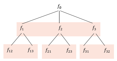
Figure 1. A finite rooted tree with $f_{\emptyset}$ as its root. The orange blocks denote subsets of polynomials that have a common interlacing. For every fixed $i$ $(i=\emptyset,1,2$ or $3)$, each polynomial $f_{i}$ is a convex combination of the polynomials $\{f_{ij}\}_{j\neq i}$. The polynomials $\{f_{ij}\}_{1\leq i\neq j\leq 3}$, which are the labels of the leaves of this tree, form an interlacing family.

The following lemma, which was proved in [20, Theorem $2.7$], shows the utility of forming an interlacing family.

Lemma 2.9 ([20], Theorem $2.7$).

Let $f$ be an interlacing family of degree $n$ polynomials with root labeled by $f_{\emptyset}(x)$ and leaves by $\{f_{v}(x)\}_{v\in\mathbb{T}}$. Then for all indices $1\leq j\leq n$, there exist leaves $v_{1}$ and $v_{2}$ such that

$$\lambda_{j}(f_{v_{1}})\geq\lambda_{j}(f_{\emptyset})\geq\lambda_{j}(f_{v_{2}}).$$

2.3. Lower barrier function

In this section, we introduce the lower barrier function from [4, 19]. For a real-rooted polynomial $p(x)$, one can use the evolution of such a barrier function to track the approximate locations of the roots of $\partial_{x}^{k}p(x)$.

Definition 2.10.

For a real-rooted polynomial $p(x)$ with roots $\lambda_{1},\ldots,\lambda_{n}$, the lower barrier function of $p(x)$ is defined as

$$\Phi_{p}(x):=-\frac{p^{\prime}(x)}{p(x)}=\sum\limits_{i=1}^{n}\frac{1}{\lambda_{i}-x}.$$

We have the following technical lemma for the lower barrier function, which can be obtained by Lemma $5.11$ in [19]. Here, we include a novel proof for completeness.

Lemma 2.11.

Suppose that $p(x)$ is a real-rooted polynomial and $\delta>0$. Suppose that $b<\lambda_{\min}(p)$ and

$$\Phi_{p}(b)\leq\frac{1}{\delta}.$$

Then

(9) $$\Phi_{\partial_{x}p}(b+\delta)\leq\Phi_{p}(b).$$

Proof.

Suppose that the degree of $p$ is $d$ and its roots are $\lambda_{d}\leq\cdots\leq\lambda_{1}$. According to the definition of $\Phi_{p}$, we have

$$\frac{1}{\lambda_{d}-b}<\Phi_{p}(b)\leq\frac{1}{\delta},$$

which implies $b+\delta<\lambda_{d}\leq\lambda_{\min}(\partial_{x}p)$. Here, we use $\lambda_{d}\leq\lambda_{\min}(\partial_{x}p)$, which can be obtained by Rolle’s theorem. Next, we express $\Phi_{\partial_{x}p}$ in terms of $\Phi_{p}$ and $(\Phi_{p})^{\prime}$:

$$\Phi_{\partial_{x}p}=-\frac{p^{\prime\prime}}{p^{\prime}}=-\frac{p^{\prime\prime}p-(p^{\prime})^{2}}{p^{\prime}p}-\frac{p^{\prime}}{p}=-\frac{(\Phi_{p})^{{}^{\prime}}}{\Phi_{p}}+\Phi_{p}.$$

wherever all quantities are finite, which happens everywhere except at the zeros of $p$ and $p^{\prime}$. Because $b+\delta$ is strictly below the zeros of both, it follows that:

$$\Phi_{\partial_{x}p}(b+\delta)=\Phi_{p}(b+\delta)-\frac{(\Phi_{p})^{\prime}(b+\delta)}{\Phi_{p}(b+\delta)}.$$

Therefore, (9) is equivalent to

$$\Phi_{p}(b+\delta)-\Phi_{p}(b)\leq\frac{(\Phi_{p})^{\prime}(b+\delta)}{\Phi_{p}(b+\delta)},$$

i.e.,

$$\Phi_{p}(b+\delta)\big{(}\Phi_{p}(b+\delta)-\Phi_{p}(b)\big{)}\leq(\Phi_{p})^{\prime}(b+\delta).$$

By expanding $\Phi_{p}$ and $(\Phi_{p})^{\prime}$ in terms of the zeros of $p$, we can see that (9) is equivalent to

(10) $$\bigg{(}\sum\limits_{i}\frac{1}{\lambda_{i}-b-\delta}\bigg{)}\bigg{(}\sum\limits_{i}\frac{1}{\lambda_{i}-b-\delta}-\sum\limits_{i}\frac{1}{\lambda_{i}-b}\bigg{)}\leq\sum\limits_{i}\frac{1}{(\lambda_{i}-b-\delta)^{2}}.$$

Noting that $\frac{1}{\lambda_{i}-b-\delta}=\frac{1}{\lambda_{i}-b}+\frac{\delta}{(\lambda_{i}-b)(\lambda_{i}-b-\delta)}$, we obtain that

$$\begin{array}[]{ll}\bigg{(}\sum\limits_{i}\frac{1}{\lambda_{i}-b-\delta}\bigg{)}\bigg{(}\sum\limits_{i}\frac{1}{\lambda_{i}-b-\delta}&-\sum\limits_{i}\frac{1}{\lambda_{i}-b}\bigg{)}=\bigg{(}\sum\limits_{i}\frac{1}{\lambda_{i}-b}+\sum\limits_{i}\frac{\delta}{(\lambda_{i}-b)(\lambda_{i}-b-\delta)}\bigg{)}\bigg{(}\sum\limits_{i}\frac{\delta}{(\lambda_{i}-b)(\lambda_{i}-b-\delta)}\bigg{)}\\ &=\bigg{(}\sum\limits_{i}\frac{\delta}{(\lambda_{i}-b)(\lambda_{i}-b-\delta)}\bigg{)}^{2}+\bigg{(}\sum\limits_{i}\frac{\delta}{\lambda_{i}-b}\bigg{)}\bigg{(}\sum\limits_{i}\frac{1}{(\lambda_{i}-b)(\lambda_{i}-b-\delta)}\bigg{)}\\ &\leq\bigg{(}\sum\limits_{i}\frac{\delta}{\lambda_{i}-b}\bigg{)}\bigg{(}\sum\limits_{i}\frac{\delta}{(\lambda_{i}-b)(\lambda_{i}-b-\delta)^{2}}\bigg{)}+\sum\limits_{i}\frac{1}{(\lambda_{i}-b)(\lambda_{i}-b-\delta)}\\ &\leq\sum\limits_{i}\frac{\delta}{(\lambda_{i}-b)(\lambda_{i}-b-\delta)^{2}}+\sum\limits_{i}\frac{1}{(\lambda_{i}-b)(\lambda_{i}-b-\delta)}\\ &=\sum\limits_{i}\frac{1}{(\lambda_{i}-b-\delta)^{2}}-\sum\limits_{i}\frac{1}{(\lambda_{i}-b)(\lambda_{i}-b-\delta)}+\sum\limits_{i}\frac{1}{(\lambda_{i}-b)(\lambda_{i}-b-\delta)}\\ &=\sum\limits_{i}\frac{1}{(\lambda_{i}-b-\delta)^{2}},\end{array}$$

which implies (10) and hence (9). Here, the first and second inequalities follow from $\Phi_{p}(b)\leq\frac{1}{\delta}$, i.e., $\sum\limits_{i}\frac{\delta}{\lambda_{i}-b}\leq 1$ and the Cauchy-Schwarz inequality, respectively. ∎

3. Proof of Theorem 1.3

In this section, we present the proof of Theorem 1.3. Our proof provides a deterministic greedy algorithm that will be presented in Section 4. To state our proof, we introduce the following result but postpone its proof till the end of this section.

Theorem 3.1.

Let $Y\in{\mathbb{R}}^{n\times(m+\ell)}$ that satisfies $YY^{T}=I$. Assume that ${\mathcal{S}}_{M}\subseteq[m+\ell]$ with $|{\mathcal{S}}_{M}|=\ell$. Let $M:=Y_{{\mathcal{S}}_{M}}\in\mathbb{R}^{n\times\ell}$ be a sub-matrix of $Y$ whose columns are indexed by ${\mathcal{S}}_{M}$. Set $r:=rank(M)$. Then for any fixed $k\in[n-r,m-1]$ there exists a subset ${\mathcal{S}}_{0}\subseteq[m+\ell]\setminus{\mathcal{S}}_{M}$ with size $k$ such that

$$\sigma_{\min}\big{(}\big{[}M\ Y_{{\mathcal{S}}_{0}}\big{]}\big{)}^{2}\geq\Gamma^{-1}(m,n,k,r)\cdot\frac{m-n+r}{m-n+\|M^{\dagger}\|_{F}^{2}},$$

where $\Gamma(m,n,k,r)$ is defined in (1).

Using Theorem 3.1, we next present the proof of Theorem 1.3.

Proof of Theorem 1.3.

Let $[A\ \,B]=U\Sigma Y$ be the SVD of $[A\ \ B]$. Suppose that ${\mathcal{S}}_{A}\subseteq[m+\ell]$ and ${\mathcal{S}}_{B}\subseteq[m+\ell]$ are two indexed sets such that $A=U\Sigma Y_{{\mathcal{S}}_{A}}$ and $B=U\Sigma Y_{{\mathcal{S}}_{B}}$.

Recall that $\mbox{rank}\big{(}[A\ B]\big{)}=n$, which implies that $YY^{T}=I_{n}$. Applying Theorem 3.1 with $M:=Y_{{\mathcal{S}}_{A}}$, we obtain that there exists a subset $\mathcal{S}_{0}\subseteq[m+\ell]\setminus{\mathcal{S}}_{A}$ with size $k\in[n-r,m-1]$ such that

(11) $$\sigma_{\min}\big{(}\big{[}Y_{{\mathcal{S}}_{A}}\ \,Y_{{\mathcal{S}}_{0}}\big{]}\big{)}^{2}\geq\Gamma^{-1}(m,n,k,r)\cdot\frac{m-n+r}{m-n+\|(Y_{{\mathcal{S}}_{A}})^{\dagger}\|^{2}_{F}}.$$

Considering the left side of (2), we have

(12) $$\big{\|}\big{(}\big{[}A\ \,B_{\mathcal{S}_{0}}\big{]}\big{)}^{\dagger}\big{\|}_{\xi}^{2}=\big{\|}\big{(}[U\Sigma Y_{{\mathcal{S}}_{A}}\ \,U\Sigma Y_{{\mathcal{S}}_{0}}]\big{)}^{\dagger}\big{\|}_{\xi}^{2}=\big{\|}\big{(}U\Sigma([Y_{{\mathcal{S}}_{A}}\ \,Y_{{\mathcal{S}}_{0}}])\big{)}^{\dagger}\big{\|}_{\xi}^{2}.$$

From (11), we know that the matrix $[Y_{{\mathcal{S}}_{A}}\ \,Y_{{\mathcal{S}}_{0}}\big{]}$ has full row rank. Since $U\Sigma$ also has full column rank, by Lemma 2.1 we know that $\mbox{rank}([A\ \,B_{\mathcal{S}_{0}}])=n$ and

(13) $$\begin{array}[]{ll}\big{\|}\big{(}U\Sigma([Y_{{\mathcal{S}}_{A}}\ \,Y_{{\mathcal{S}}_{0}}])\big{)}^{\dagger}\big{\|}_{\xi}^{2}&=\big{\|}([Y_{{\mathcal{S}}_{A}}\ \,Y_{{\mathcal{S}}_{0}}])^{\dagger}\Sigma^{-1}U^{T}\big{\|}_{\xi}^{2}\\[5.69054pt] &\overset{(a)}{\leq}\big{\|}([Y_{{\mathcal{S}}_{A}}\ \,Y_{{\mathcal{S}}_{0}}])^{\dagger}\big{\|}_{2}^{2}\cdot\big{\|}([A\ \,B])^{\dagger}\big{\|}_{\xi}^{2}\\[5.69054pt] &\overset{(b)}{\leq}\Gamma(m,n,k,r)\cdot\frac{m-n+\|(Y_{{\mathcal{S}}_{A}})^{\dagger}\|^{2}_{F}}{m-n+r}\cdot\big{\|}([A\ \,B])^{\dagger}\big{\|}_{\xi}^{2},\end{array}$$

where $(a)$ follows from the standard properties of matrix norms and using the definition of the pseudoinverse of $[A\ \,B]$ and $\Sigma$, and $(b)$ follows from (11). To complete the proof, we still need to present an upper bound on $\|(Y_{{\mathcal{S}}_{A}})^{\dagger}\|^{2}_{F}$. Note that

(14) $$\begin{array}[]{ll}\|(Y_{{\mathcal{S}}_{A}})^{\dagger}\|^{2}_{F}\overset{(a)}{=}\|(\Sigma^{-1}U^{T}A)^{\dagger}\|^{2}_{F}&\overset{(b)}{\leq}\|A^{\dagger}U\Sigma\|^{2}_{F}\\ &\overset{(c)}{=}\|A^{\dagger}U\Sigma YY^{T}\|^{2}_{F}\\ &\overset{(d)}{\leq}\|A^{\dagger}[A\ \,B]\|^{2}_{F}\\ &\overset{(e)}{=}r+\|A^{\dagger}B\|^{2}_{F},\end{array}$$

where $(a)$ follows from $A=U\Sigma Y_{{\mathcal{S}}_{A}}$, $(b)$ follows from Lemma 2.2, $(c)$ follows from $YY^{T}=I$, $(d)$ follows from $U\Sigma Y=[A\ \,B]$, the standard properties of matrix norms, and $\|Y^{T}\|_{2}\leq 1$, and $(e)$ follows from $\mbox{rank}(A)=r$. Thus, combining (12), (13), and (14), we arrive at (2). ∎

The remainder of this section aims to prove Theorem 3.1. The proof consists of two parts. We first prove that the characteristic polynomials of the matrices that arise in Theorem 3.1 form an interlacing family. Secondly, we use the barrier function argument to establish a lower bound on the smallest zero of the expected characteristic polynomial.

3.1. An interlacing family for subset selection

Let the columns of $Y$ be the vectors $y_{1},\ldots,y_{m+\ell}\in\mathbb{R}^{n}$, and let $M=Y_{{\mathcal{S}}_{M}}$ be a given matrix with $\mbox{rank}(M)=r$. Since $YY^{T}=I$, we obtain that $\sum\limits_{i=1}^{m+\ell}y_{i}y_{i}^{T}=I$. Denote the nonzero singular values of $M$ as $\sigma_{1}(M),\ldots,\sigma_{r}(M)$. For each ${\mathcal{S}}\subseteq[m+\ell]\setminus{\mathcal{S}}_{M}$, set

$$p^{M}_{{\mathcal{S}}}(x):=\det[xI-Y_{{\mathcal{S}}}Y^{T}_{{\mathcal{S}}}-MM^{T}].$$

For a fixed set $\mathcal{T}$ with size less than $k$, we define the polynomial

(15) $$f^{M}_{\mathcal{T}}(x):=\mathop{\mathbb{E}}\limits_{{\mathcal{S}}\supseteq\mathcal{T},|{\mathcal{S}}|=k\atop{\mathcal{S}}\subseteq[m+\ell]\setminus{\mathcal{S}}_{M}}p^{M}_{{\mathcal{S}}}(x),$$

where the expectation is taken uniformly over sets ${\mathcal{S}}\subseteq[m+\ell]\setminus{\mathcal{S}}_{M}$ with size $k$ containing $\mathcal{T}$. Building on the ideas of Marcus-Spielman-Srivastava [20], we can derive expressions for the polynomials $f^{M}_{\mathcal{T}}(x)$.

We begin with the following result.

Lemma 3.2.

Suppose that $p^{M}_{{\mathcal{S}}}(x)=\det[xI-Y_{{\mathcal{S}}}Y^{T}_{{\mathcal{S}}}-MM^{T}]$. Then

$$\sum\limits_{i\notin\mathcal{S}\cup{\mathcal{S}}_{M}}p^{M}_{\mathcal{S}\cup\{i\}}(x)=(x-1)^{-(m-n-t-1)}\partial_{x}(x-1)^{m-n-t}p^{M}_{\mathcal{S}}(x)$$

holds for every subset $\mathcal{S}\subseteq[m+\ell]\setminus{\mathcal{S}}_{M}$ with size $t$.

Proof.

According to Lemma 2.5, we have

$$\begin{array}[]{ll}\sum\limits_{i\notin\mathcal{S}\cup{\mathcal{S}}_{M}}p^{M}_{\mathcal{S}\cup\{i\}}(x)&=\sum\limits_{i\notin\mathcal{S}\cup{\mathcal{S}}_{M}}\det\big{[}xI-Y_{{\mathcal{S}}}Y^{T}_{{\mathcal{S}}}-y_{i}y_{i}^{T}-MM^{T}\big{]}\\[5.69054pt] &=\sum\limits_{i\notin\mathcal{S}\cup{\mathcal{S}}_{M}}\det\big{[}xI-Y_{{\mathcal{S}}}Y^{T}_{{\mathcal{S}}}-MM^{T}\big{]}\big{(}1-\mbox{Tr}\big{[}(xI-Y_{{\mathcal{S}}}Y^{T}_{{\mathcal{S}}}-MM^{T})^{-1}y_{i}y_{i}^{T}\big{]}\big{)}.\end{array}$$

Because $p^{M}_{\mathcal{S}}(x)=\det[xI-Y_{{\mathcal{S}}}Y^{T}_{{\mathcal{S}}}-MM^{T}]$ and $\sum\limits_{i\notin\mathcal{S}\cup{\mathcal{S}}_{M}}y_{i}y_{i}^{T}=I-Y_{{\mathcal{S}}}Y^{T}_{{\mathcal{S}}}-MM^{T}$, we obtain that

$$\begin{array}[]{ll}\sum\limits_{i\notin\mathcal{S}\cup{\mathcal{S}}_{M}}p^{M}_{\mathcal{S}\cup\{i\}}(x)&=p^{M}_{\mathcal{S}}(x)\big{(}m-t-\mbox{Tr}\big{[}(xI-Y_{{\mathcal{S}}}Y^{T}_{{\mathcal{S}}}-MM^{T})^{-1}(I-Y_{{\mathcal{S}}}Y^{T}_{{\mathcal{S}}}-MM^{T})\big{]}\big{)}\\[5.69054pt] &=p^{M}_{\mathcal{S}}(x)(m-t)-p^{M}_{\mathcal{S}}(x)\mbox{Tr}\big{[}\big{(}xI-Y_{{\mathcal{S}}}Y^{T}_{{\mathcal{S}}}-MM^{T}\big{)}^{-1}\\[2.84526pt] &\ \ \ \times\big{(}(I-xI)+(xI-Y_{{\mathcal{S}}}Y^{T}_{{\mathcal{S}}}-MM^{T})\big{)}\big{]}\\[5.69054pt] &=p^{M}_{\mathcal{S}}(x)(m-t)-np^{M}_{\mathcal{S}}(x)-p^{M}_{\mathcal{S}}(x)\mbox{Tr}\big{[}(xI-Y_{{\mathcal{S}}}Y^{T}_{{\mathcal{S}}}-MM^{T})^{-1}(I-xI)\big{]}\\[5.69054pt] &=p^{M}_{\mathcal{S}}(x)(m-t-n)-p^{M}_{\mathcal{S}}(x)\mbox{Tr}\big{[}(xI-Y_{{\mathcal{S}}}Y^{T}_{{\mathcal{S}}}-MM^{T})^{-1}\big{]}(1-x)\\[5.69054pt] &\overset{(a)}{=}(m-n-t)p^{M}_{\mathcal{S}}(x)+(x-1)\partial_{x}p^{M}_{\mathcal{S}}(x)\\[5.69054pt] &=(x-1)^{-(m-n-t-1)}\partial_{x}(x-1)^{m-n-t}p^{M}_{\mathcal{S}}(x),\end{array}$$

where $(a)$ follows from Lemma 2.3. ∎

Motivated by Lemma $5.3$ in [20], we give expressions for $f^{M}_{\mathcal{T}}(x)$ in the following lemma:

Lemma 3.3.

Suppose that $\mathcal{T}\subseteq[m+\ell]\setminus{\mathcal{S}}_{M}$ with size $t\leq k$. Then

$$f_{\mathcal{T}}^{M}(x)=\frac{1}{{m-t\choose k-t}}\sum\limits_{{\mathcal{S}}\supseteq\mathcal{T},|{\mathcal{S}}|=k\atop{\mathcal{S}}\subseteq[m+\ell]\setminus{\mathcal{S}}_{M}}p_{{\mathcal{S}}}^{M}(x)=\frac{(m-k)!}{(m-t)!}(x-1)^{-(m-n-k)}\partial_{x}^{k-t}(x-1)^{m-n-t}p^{M}_{\mathcal{T}}(x),$$

where $p^{M}_{\mathcal{T}}(x)=\det[xI-Y_{\mathcal{T}}Y^{T}_{\mathcal{T}}-MM^{T}]$. In particular,

$$f^{M}_{\emptyset}(x)=\frac{(m-k)!}{m!}(x-1)^{-(m-n-k)}\partial_{x}^{k}(x-1)^{m-n}x^{n-r}\prod\limits_{i=1}^{r}\big{(}x-\sigma_{i}(M)^{2}\big{)}.$$

Proof.

To prove this lemma, it is sufficient to show that

(16) $$\sum\limits_{{\mathcal{S}}\supseteq\mathcal{T},|{\mathcal{S}}|=k\atop{\mathcal{S}}\subseteq[m+\ell]\setminus{\mathcal{S}}_{M}}p^{M}_{{\mathcal{S}}}(x)=\frac{1}{(k-t)!}(x-1)^{-(m-n-k)}\partial_{x}^{k-t}(x-1)^{m-n-t}p^{M}_{\mathcal{T}}(x).$$

We prove (16) by induction on $k$. For $k=t$, a simple calculation shows that (16) holds. For $k>t$, we have

$$\sum\limits_{{\mathcal{S}}\supseteq\mathcal{T},|{\mathcal{S}}|=k\atop{\mathcal{S}}\subseteq[m+\ell]\setminus{\mathcal{S}}_{M}}p^{M}_{{\mathcal{S}}}(x)=\frac{1}{k-t}\sum\limits_{{\mathcal{S}}\supseteq\mathcal{T},|{\mathcal{S}}|=k-1\atop{\mathcal{S}}\subseteq[m+\ell]\setminus{\mathcal{S}}_{M}}\sum\limits_{i\notin{\mathcal{S}}\cup{\mathcal{S}}_{M}}p^{M}_{{\mathcal{S}}\cup\{i\}}(x).$$

Hence by induction and Lemma 3.2, we have

$$\begin{array}[]{ll}\sum\limits_{{\mathcal{S}}\supseteq\mathcal{T},|{\mathcal{S}}|=k\atop{\mathcal{S}}\subseteq[m+\ell]\setminus{\mathcal{S}}_{M}}p^{M}_{{\mathcal{S}}}(x)&=\frac{1}{k-t}\sum\limits_{{\mathcal{S}}\supseteq\mathcal{T},|{\mathcal{S}}|=k-1\atop{\mathcal{S}}\subseteq[m+\ell]\setminus{\mathcal{S}}_{M}}(x-1)^{-(m-n-(k-1)-1)}\partial_{x}(x-1)^{m-n-(k-1)}p^{M}_{\mathcal{S}}(x)\\[22.76219pt] &=\frac{1}{k-t}(x-1)^{-(m-n-(k-1)-1)}\partial_{x}\bigg{(}(x-1)^{m-n-(k-1)}\sum\limits_{{\mathcal{S}}\supseteq\mathcal{T},|{\mathcal{S}}|=k-1\atop{\mathcal{S}}\subseteq[m+\ell]\setminus{\mathcal{S}}_{M}}p^{M}_{\mathcal{S}}(x)\bigg{)}\\[22.76219pt] &=\frac{1}{k-t}(x-1)^{-(m-n-(k-1)-1)}\partial_{x}\big{(}(x-1)^{m-n-(k-1)}\\ &\ \ \ \times\frac{1}{(k-1-t)!}(x-1)^{-(m-n-(k-1))}\partial_{x}^{k-1-t}(x-1)^{m-n-t}p^{M}_{\mathcal{T}}(x)\big{)}\\[12.80373pt] &=\frac{1}{(k-t)!}(x-1)^{-(m-n-k)}\partial_{x}^{k-t}(x-1)^{m-n-t}p^{M}_{\mathcal{T}}(x).\end{array}$$

This completes the proof of this lemma. ∎

When $M=0$, Marcus, Spielman and Srivastava [20, Theorem $5.4$] proved that the polynomials $p_{{\mathcal{S}}}(x):=p^{0}_{{\mathcal{S}}}(x)$ for $|{\mathcal{S}}|=k$ form an interlacing family. Inspired by the arguments of Marcus-Spielman-Srivastava in [20], we prove that the polynomials $p^{M}_{\mathcal{{\mathcal{S}}}}(x)$ for $|{\mathcal{S}}|=k$ still satisfy the requirements of interlacing families.

Theorem 3.4.

The polynomials $p^{M}_{{\mathcal{S}}}(x)=\det\big{[}xI-Y_{{\mathcal{S}}}Y^{T}_{{\mathcal{S}}}-MM^{T}\big{]}$ for $|{\mathcal{S}}|=k$ are an interlacing family.

Proof.

We construct a tree $\mathbb{T}$ whose nodes are $\mathcal{T}\subseteq[m+\ell]\setminus{\mathcal{S}}_{M}$ (possibly empty) with size less than or equal to $k$. The node $\mathcal{T}_{1}$ is a child of $\mathcal{T}_{2}$ if and only if $\mathcal{T}_{2}\subset\mathcal{T}_{1}$ and $\lvert\mathcal{T}_{1}\setminus\mathcal{T}_{2}\rvert=1$. For an internal node $\mathcal{T}\subseteq[m+\ell]\setminus{\mathcal{S}}_{M}$ (possibly empty) with size less than $k$, we label $\mathcal{T}$ by the polynomial $f^{M}_{\mathcal{T}}(x)$, which is defined in (15). Similarly, we label the leaves of $\mathbb{T}$ as $p^{M}_{{\mathcal{S}}}(x)$ with $\lvert{\mathcal{S}}\rvert=k$. Note that the polynomials $p^{M}_{{\mathcal{S}}}(x)$ are real-rooted and monic, which implies that the polynomials $f^{M}_{\mathcal{T}}(x)$ are also monic as they are the averages of $p^{M}_{\mathcal{S}}(x)$ with ${\mathcal{S}}\subseteq[m+\ell]\setminus{\mathcal{S}}_{M}$ with size $k$ containing $\mathcal{T}$. We will show that the polynomials $f^{M}_{\mathcal{T}}(x)$ are real-rooted later. Now we already constructed the finite rooted tree $\mathbb{T}$, where $f^{M}_{\emptyset}(x)$ is the root of the tree.

We already showed that the tree $\mathbb{T}$ satisfies $(a)$ in Definition 2.8. We next show that $\mathbb{T}$ also satisfies condition $(b)$.

Suppose that $\mathcal{T}\subseteq[m+\ell]\setminus{\mathcal{S}}_{M}$ with size less than $k$. To complete the proof, by Lemma 2.7, we need to prove that all convex combinations of $f^{M}_{\mathcal{T}\cup\{i\}}$ and $f^{M}_{\mathcal{T}\cup\{j\}}$ are real-rooted for every $i,j\notin\mathcal{T}\cup{\mathcal{S}}_{M}$. That is, we must prove that the polynomial

$$q_{\mu}(x):=\mu f^{M}_{\mathcal{T}\cup\{i\}}(x)+(1-\mu)f^{M}_{\mathcal{T}\cup\{j\}}(x)$$

is real-rooted for each $0\leq\mu\leq 1$. Let

$$h_{\mu}(x):=\mu p^{M}_{\mathcal{T}\cup\{i\}}(x)+(1-\mu)p^{M}_{\mathcal{T}\cup\{j\}}(x).$$

It follows from Lemma 2.7 that the polynomials $p^{M}_{\mathcal{T}\cup\{i\}}$ and $p^{M}_{\mathcal{T}\cup\{j\}}$ have a common interlacing. Hence, by Lemma 2.6, we have that $h_{\mu}(x)$ is real-rooted. According to Lemma 3.3, we obtain that

$$q_{\mu}(x)=\frac{(m-k)!}{(m-t)!}(x-1)^{-(m-n-k)}\partial_{x}^{k-t}(x-1)^{m-n-t}h_{\mu}(x).$$

Noting the real rootedness can be preserved by multiplication by $(x-1)$, taking derivatives, and dividing by $(x-1)$ when $1$ is a root, we can obtain that $q_{\mu}(x)$ is real-rooted. ∎

3.2. Proof of Theorem 3.1

The aim of this subsection is to prove Theorem 3.1. We first establish a lower bound on the smallest zero of $f^{M}_{\emptyset}(x)$ using the lower barrier function.

Lemma 3.5.

Suppose that $M\in{\mathbb{R}}^{n\times\ell}$ with nonzero singular values $\sigma_{1},\ldots,\sigma_{r}\in(0,1]$. For $n-r\leq k\leq m-1$, let

$$f^{M}_{\emptyset}(x)=\frac{(m-k)!}{m!}(x-1)^{-(m-n-k)}\partial_{x}^{k}(x-1)^{m-n}x^{n-r}\prod\limits_{i=1}^{r}\big{(}x-\sigma_{i}^{2}\big{)}.$$

Then

$$\lambda_{\min}(f^{M}_{\emptyset})\geq\Gamma^{-1}(m,n,k,r)\cdot\frac{m-n+r}{m-n+\|M^{\dagger}\|^{2}_{F}},$$

where $\lambda_{\min}(f^{M}_{\emptyset})$ denotes the smallest zero of $f^{M}_{\emptyset}$ and $\Gamma(m,n,k,r)$ is defined in (1).

Proof.

Let

$$g(x):=\partial_{x}^{k}(x-1)^{m-n}x^{n-r}\prod\limits_{i=1}^{r}\big{(}x-\sigma_{i}^{2}\big{)}$$

and

$$p(x):=(x-1)^{m-n}x^{n-r}\prod\limits_{i=1}^{r}\big{(}x-\sigma_{i}^{2}\big{)}.$$

By Rolle’s theorem, we know that $\partial_{x}p$ interlaces $p$. Thus, applying this fact $k$ times and noting that all the zeros of $p(x)$ belong to $[0,1]$, we conclude that all the zeros of $g(x)$ are between $0$ and $1$, which implies that $\lambda_{\min}(f^{M}_{\emptyset})=\lambda_{\min}(g)$. Thus, it is sufficient to prove that

$$\lambda_{\min}(g)\geq\Gamma^{-1}(m,n,k,r)\cdot\frac{m-n+r}{m-n+\sum\limits_{i=1}^{r}\frac{1}{\sigma_{i}^{2}}}.$$

For convenience, we set

$$\Lambda:=\Lambda(m,n,r,\sigma):=\frac{m-n+r}{m-n+\sum\limits_{i=1}^{r}\frac{1}{\sigma_{i}^{2}}}.$$

For any $\delta>0$, let

$$b:=b(\delta):=\frac{(\Lambda-m\delta)-\sqrt{(\Lambda-m\delta)^{2}+4\delta\Lambda(n-r)}}{2}.$$

Note that $b<\lambda_{\rm min}(p)$. We claim that

(17) $$\Phi_{g}(b+k\delta)\leq\frac{1}{\delta}.$$

Indeed, according to the definition of the lower barrier function of $p$, we obtain that

(18) $$\begin{array}[]{ll}\Phi_{p}(b)=-\frac{p^{\prime}}{p}&=\frac{m-n}{-b+1}+\sum\limits_{i=1}^{r}\frac{1}{-b+\sigma_{i}^{2}}+\frac{n-r}{-b}\\[17.07164pt] &=(m-n+r)\bigg{(}\frac{1}{m-n+r}\cdot\frac{m-n}{-b+1}+\frac{1}{m-n+r}\sum\limits_{i=1}^{r}\frac{1}{-b+\sigma_{i}^{2}}\bigg{)}+\frac{n-r}{-b}\\[17.07164pt] &\leq\frac{m-n+r}{-b+\frac{1}{\frac{1}{m-n+r}\big{(}m-n+\sum\limits_{i=1}^{r}\frac{1}{\sigma_{i}^{2}}\big{)}}}+\frac{n-r}{-b}=\frac{m-n+r}{-b+\Lambda}+\frac{n-r}{-b}\\[22.76219pt] &=\frac{1}{\delta},\end{array}$$

where the inequality follows from Lemma 2.4 with the fact the function $x\to\frac{1}{-b+\frac{1}{x}}$ is concave on $(0,+\infty)$. Applying Lemma 2.11 $k$ times, we obtain

$$\Phi_{g}(b+k\delta)\leq\Phi_{p}(b)\leq\frac{1}{\delta},$$

which implies (17). Noting that

$$\frac{1}{\lambda_{\min}(g)-(b+k\delta)}\leq\Phi_{g}(b+k\delta)\leq\frac{1}{\delta},$$

we obtain that

(19) $$\lambda_{\min}(g)\geq b+(k+1)\delta,$$

i.e.,

(20) $$\lambda_{\min}(g)\geq\mu(\delta):=\frac{(\Lambda-m\delta)-\sqrt{(\Lambda-m\delta)^{2}+4\delta\Lambda(n-r)}}{2}+(k+1)\delta.$$

Now we derive the value of $\delta$ at which $\mu(\delta)$ is maximized. Taking derivatives in $\delta$, we obtain that

$$\mu^{\prime}(\delta)=k+1-\frac{m}{2}-\frac{m^{2}\delta-m\Lambda+2\Lambda(n-r)}{2\sqrt{(\Lambda-m\delta)^{2}+4\delta\Lambda(n-r)}}.$$

As $n-r\leq k\leq m-1$, we know that

$$\mu^{\prime}(0)=k+1-(n-r)\geq 0\ \ \mbox{and }\ \ \lim\limits_{\delta\to\infty}\mu^{\prime}(\delta)=k+1-m\leq 0.$$

By continuity, a maximum will occur at a point $\delta^{*}\geq 0$ at which $\mu^{\prime}(\delta^{*})=0$. The solution is given by

$$\delta^{*}=\frac{m\Lambda-2\Lambda(n-r)}{m^{2}}-\frac{m-2(k+1)}{m^{2}}\sqrt{\frac{\Lambda^{2}(n-r)(m-n+r)}{(k+1)(m-k-1)}},$$

which is positive for $m>k\geq n-r$. Observing that

$$(\Lambda-m\delta^{*})^{2}+4\delta^{*}\Lambda(n-r)=\frac{\Lambda^{2}(n-r)(m-n+r)}{(k+1)(m-k-1)}$$

and by calculation, we can obtain that

(21) $$\mu(\delta^{*})=\Gamma^{-1}(m,n,k,r)\cdot\Lambda.$$

Combining (20) and (21), we obtain the lemma. ∎

Now we are ready to prove Theorem 3.1.

Proof of Theorem 3.1.

According to Theorem 3.4, the polynomials $p^{M}_{{\mathcal{S}}}(x)$ with $|{\mathcal{S}}|=k$ form an interlacing family. Lemma 2.9 implies that there exists a subset ${\mathcal{S}}_{0}\subseteq[m+\ell]\setminus{\mathcal{S}}_{M}$ such that $\lvert{\mathcal{S}}_{0}\rvert=k$ and

$$\lambda_{\min}\big{(}f^{M}_{{\mathcal{S}}_{0}}\big{)}\geq\lambda_{\min}\big{(}f^{M}_{\emptyset}\big{)}\geq\Gamma^{-1}(m,n,k)\cdot\frac{m-n+r}{m-n+\|M^{\dagger}\|^{2}_{F}}.$$

Here, the second inequality follows from Lemma 3.5. As $f^{M}_{{\mathcal{S}}_{0}}$ is the characteristic polynomial of $MM^{T}+Y_{{\mathcal{S}}_{0}}Y_{{\mathcal{S}}_{0}}^{T}$, we conclude that there exists a subset ${\mathcal{S}}_{0}\subseteq[m+\ell]\setminus{\mathcal{S}}_{M}$ with size $k$ for which

$$\sigma_{\min}\big{(}\big{[}M\ Y_{{\mathcal{S}}_{0}}\big{]}\big{)}^{2}=\lambda_{\min}\bigg{(}MM^{T}+Y_{{\mathcal{S}}_{0}}Y_{{\mathcal{S}}_{0}}^{T}\bigg{)}\geq\Gamma^{-1}(m,n,k)\cdot\frac{m-n+r}{m-n+\|M^{\dagger}\|^{2}_{F}}.$$

∎

4. A deterministic greedy selection algorithm

The aim of this section is to present a deterministic greedy selection algorithm for Problem 1.2. The proposed algorithm is based on the proof of the main result. Suppose that $A\in\mathbb{R}^{n\times\ell}$ and $B\in\mathbb{R}^{n\times m}$ with $\mbox{rank}([A\ \ B])=n$. Let the SVD of $[A\ \,B]$ be $U\Sigma Y$, where $Y=[Y_{{\mathcal{S}}_{A}}\ \,Y_{{\mathcal{S}}_{B}}]$ and ${\mathcal{S}}_{A}$ and ${\mathcal{S}}_{B}$ denote the column set of matrices $A$ and $B$, respectively. Assume that $M:=Y_{{\mathcal{S}}_{A}}$ and $Y=[y_{1},\ldots,y_{m+\ell}]$. Given a partial assignment $\{s_{1},\ldots,s_{j}\}\subseteq{\mathcal{S}}_{B}$, from Lemma 3.3, we set the polynomial corresponding to $\{s_{1},\ldots,s_{j}\}$ as

(22) $$f^{M}_{s_{1},\ldots,s_{j}}(x):=\frac{(m-k)!}{(m-j)!}(x-1)^{-(m-n-k)}\partial_{x}^{k-j}(x-1)^{m-n-j}p^{M}_{s_{1},\ldots,s_{j}}(x),$$

where $p^{M}_{s_{1},\ldots,s_{j}}(x)=\det\bigg{[}xI-\sum\limits_{i=1}^{j}{y_{s_{i}}y^{T}_{s_{i}}}-MM^{T}\bigg{]}$. The algorithm produces the subset $\mathcal{S}_{0}$ in polynomial time by iteratively adding columns to it. Namely, suppose that at the $(i-1)$-th ($1\leq i\leq k$) iteration, we have already found a partial assignment $s_{1},\ldots,s_{i-1}$ (which is empty when $i=1$). Now, at the $i$-th iteration, the algorithm finds an index $s_{i}\in{\mathcal{S}}_{B}\setminus\{s_{1},\ldots,s_{i-1}\}$ such that $\lambda_{\min}(f^{M}_{s_{1},\ldots,s_{i}})\geq\lambda_{\min}(f^{M}_{s_{1},\ldots,s_{i-1}})$.

Let $p(x)$ be a given real-rooted polynomial; we use $\lambda^{\epsilon}_{\min}\big{(}p(x)\big{)}$ to denote an $\epsilon$-approximation to the smallest root of $p(x)$, i.e.,

$$\big{|}\lambda^{\epsilon}_{\min}\big{(}p(x)\big{)}-\lambda_{\min}\big{(}p(x)\big{)}\big{|}\leq\epsilon.$$

The deterministic greedy selection algorithm can be stated as follows:

Algorithm 1 Deterministic greedy selection algorithm

$B\in\mathbb{R}^{n\times m}$ of rank $n$; $A\in\mathbb{R}^{n\times\ell}$; sampling parameter $k\in\{n-\mbox{rank}(A),\ldots,m-1\}$.

1. Set $s_{0}=\emptyset$ and $i:=1$.

2. Compute the thin SVD of $[A\ \,B]=U\Sigma Y$ with $Y=[Y_{{\mathcal{S}}_{A}}\ \,Y_{{\mathcal{S}}_{B}}]$.

3. Let $M:=Y_{{\mathcal{S}}_{A}}$ and $Y=[y_{1},\ldots,y_{m+\ell}]\in\mathbb{R}^{n\times(m+\ell)}$.

4. Using the standard technique of binary search with a Sturm sequence, for each $s\in{\mathcal{S}}_{B}\setminus\{s_{1},\ldots,s_{i-1}\}$, compute an $\epsilon$-approximation to the smallest root of $f^{M}_{s_{1},\ldots,s_{i-1},s}(x)$.

5. Find

   $$s_{i}=\mathop{\rm argmax}\limits_{s\in{\mathcal{S}}_{B}\setminus\{s_{1},\ldots,s_{i-1}\}}\lambda^{\epsilon}_{\min}\big{(}f^{M}_{s_{1},\ldots,s_{i-1},s}(x)\big{)}.$$

6. If $i>k$, stop the algorithm. Otherwise, set $i=i+1$ and return to Step $4$.

Subset ${\mathcal{S}}_{0}=\{s_{1},\ldots,s_{k}\}.$

We have the following theorem for Algorithm $1$.

Theorem 4.1.

Suppose that $0<\epsilon<\frac{1}{2k}$. Algorithm $1$ can output a subset ${\mathcal{S}}_{0}=\{s_{1},\ldots,s_{k}\}$ such that

(23) $$\big{\|}\big{(}[A\ B_{\mathcal{S}_{0}}]\big{)}^{\dagger}\big{\|}_{\xi}^{2}\leq\Gamma(m,n,k,r)\bigg{(}1+\frac{\|A^{\dagger}B\|^{2}_{F}}{m-n+r}\bigg{)}\left(1+2k\epsilon\right)\cdot\big{\|}([A\ \,B])^{\dagger}\big{\|}_{\xi}^{2}.$$

The running time complexity is $O(k(m-\frac{k}{2})n^{\theta}\log(1/\epsilon))$, where $\theta\in(2,2.373)$ is the matrix multiplication complexity exponent.

Proof.

By Step $4$ in Algorithm $1$, we obtain that

$$\lambda_{\min}\big{(}f^{M}_{s_{1},\ldots,s_{k}}(x)\big{)}\geq\lambda_{\min}\big{(}f^{M}_{s_{1},\ldots,s_{k-1}}(x)\big{)}-\epsilon\geq\cdots\geq\lambda_{\min}\big{(}f^{M}_{s_{1}}(x)\big{)}-(k-1)\epsilon\geq\lambda_{\min}\big{(}f^{M}_{\emptyset}(x)\big{)}-k\epsilon.$$

Then, using a similar argument for Theorem 1.3, we can obtain the bound (23). We next establish the running time complexity.

The main cost of Algorithm $1$ is Steps $2$ and $4$. In Step $2$, the time complexity for the computation of the SVD of $[A\ \,B]$ is $O\big{(}(m+\ell)n^{2}\big{)}$. For Step $4$, at the $i$-th iteration, we claim the time complexity for computing $\lambda^{\epsilon}_{\min}\big{(}f^{M}_{s_{1},\ldots,s_{i-1},s}(x)\big{)}$ over all $s\in{\mathcal{S}}_{B}\setminus\{s_{1},\ldots,s_{i-1}\}$ is $O((m-i+1)n^{\theta}\log(1/\epsilon))$. Therefore, Algorithm $1$ can produce the subset $\mathcal{S}_{0}$ in $O(k(m-\frac{k}{2})n^{\theta}\log(1/\epsilon))$ time.

Indeed, at the $i$-th iteration, the main cost of Step $4$ consists of (i) the computations of $f^{M}_{s_{1},\ldots,s_{i}}(x)$ and (ii) the computations of an $\epsilon$-approximation to the smallest root of $f^{M}_{s_{1},\ldots,s_{i}}(x)$ for every $s_{i}\in{\mathcal{S}}_{B}\setminus\{s_{1},\ldots,s_{i-1}\}$. First, for any $\{s_{1},\ldots,s_{j}\}\subseteq{\mathcal{S}}_{B}$, we can compute the characteristic polynomial $p^{M}_{s_{1},\ldots,s_{j}}(x)$ in $O(n^{\theta}\log n)$ time, where $2<\theta<2.373$ is an admissible exponent of matrix multiplication [17, 16]. From (22), we know that the time complexity for the computation of $f^{M}_{s_{1},\ldots,s_{j}}(x)$ is $O(n^{\theta}\log n)$ as its main cost is to compute $p^{M}_{s_{1},\ldots,s_{j}}(x)$. Therefore, the running time for computing $f^{M}_{s_{1},\ldots,s_{i}}(x)$ over all $s_{i}\in{\mathcal{S}}_{B}\setminus\{s_{1},\ldots,s_{i-1}\}$, which has $m-i+1$ choices, is $O((m-i+1)n^{\theta}\log n)$.

Secondly, for any $\{s_{1},\ldots,s_{j}\}\subseteq{\mathcal{S}}_{B}$, we can compute an $\epsilon$-approximation to the smallest root of $f^{M}_{s_{1},\ldots,s_{j}}(x)$ using the standard technique of binary search with a Sturm sequence. This takes $O(n^{2}\log(1/\epsilon))$ time per polynomial (see, e.g., [3]). Noting that $O((m-i+1)n^{\theta}\log n)+O((m-i+1)n^{2}\log(1/\epsilon))=O((m-i+1)n^{\theta}\log(1/\epsilon))$, we obtain that the time complexity of Step $4$ is $O((m-i+1)n^{\theta}\log(1/\epsilon))$. ∎

References

- [1] M. Arioli and I.S. Duff, Preconditioning of linear least-squares problems by identifying basic variables, SIAM J. Sci. Comput., 37 (2015), pp. S544-S561.
- [2] H. Avron and C. Boutsidis, Faster subset selection for matrices and applications, SIAM J. Matrix Anal. Appl., 24 (2013), pp. 1464–1499.
- [3] S. Basu, R. Pollack, and M.F. Coste-Roy, Algorithms in real algebraic geometry, Springer Science & Business Media, 2007.
- [4] J.D. Batson, D. A. Spielman, and N. Srivastava, Twice-Ramanujan sparsifiers, SIAM Review, 56 (2014), pp. 315–334.
- [5] D.S. Bernstein, Matrix mathematics: Theory, facts, and formulas with application to linear systems theory, Princeton: Princeton university press, 2005.
- [6] J. Bourgain and L. Tzafriri, Invertibility of large submatrices with applications to the geometry of Banach spaces and harmonic analysis, Israel J. Math., 57 (1987), pp. 137–224.
- [7] C. Boutsidis and M. Magdon-Ismail, Deterministic feature selection for -means clustering, IEEE Trans. Inform. Theory, 59 (2013), pp. 6099-6110.
- [8] C. Boutsidis, A. Zouzias, M.W. Mahoney, and P. Drineas, Stochastic dimensionality reduction for -means clustering. CoRR, abs/1110.2897, 2011.
- [9] S. Chen, R. Varma, A. Sandryhaila, and J. Kovaǒević, Discrete Signal Processing on Graphs: Sampling Theory. IEEE Trans. Signal Process., 63 (2015), pp. 6510-6523.
- [10] M. Chudnovsky and P. Seymour, The roots of the independence polynomial of a clawfree graph, J. Comb. Theory, Series B, 97 (2007), pp. 350-357.
- [11] A. Çivril and M. Magdon-Ismail, On selecting a maximum volume sub-matrix of a matrix and related problems, Theoret. Comput. Sci., 410 (2009), pp. 4801–4811.
- [12] M. Dereziński and M.K. Warmuth, Reverse iterative volume sampling for linear regression, J. Mach. Learn. Res., 19 (2018), pp. 1–39.
- [13] R.R. de Hoog and R.M.M. Mattheij, Subset selection for matrices, Linear Algebra Appl., 422 (2007), pp. 349–359.
- [14] R.R. de Hoog and R.M.M Mattheij, A note on subset selection for matrices, Linear Algebra Appl., 434 (2011), pp. 1845–1850.
- [15] S. Joshi and S. Boyd, Sensor selection via convex optimization, IEEE Trans. Signal Process., 57 (2009), pp. 451–462.
- [16] W. Keller-Gehrig, Fast algorithms for the characteristics polynomial, Theoret. Comput. Sci., 36 (1985), pp. 309-317.
- [17] F. Le Gall, Powers of tensors and fast matrix multiplication, Proceedings of the 39th International symposium on symbolic and algebraic computation. ACM, 2014, pp. 296-303.
- [18] A. W. Marcus, D. A. Spielman, and N. Srivastava, Interlacing Families I: Bipartite Ramanujan graphs of all degrees, Ann. of Math., 182 (2015), pp. 307–325.
- [19] A. W. Marcus, D. A. Spielman, and N. Srivastava, Interlacing Families II: Mixed characteristic polynomials and the Kadison–Singer problem, Ann. of Math. 182 (2015), pp. 327–350.
- [20] A. W. Marcus, D. A. Spielman, and N. Srivastava, Interlacing Families III: Sharper restricted invertibility estimates, arXiv: 1712.07766, 2017, to appear in Israel J. Math..
- [21] A. W. Marcus, D. A. Spielman, and N. Srivastava, Interlacing Families IV: Bipartite Ramanujan graphs of all sizes, SIAM J. Comput., 47 (2018), pp. 2488-2509.
- [22] A. W. Marcus, D. A. Spielman, and N. Srivastava, Finite free convolutions of polynomials, arXiv: 1504.00350, 2015.
- [23] A. Naor and P. Youssef, Restricted invertibility revisited, In A Journey Through Discrete Mathematics, Springer, 2017, pp. 657–691.
- [24] F. Pukelsheim, Optimal design of experiments, SIAM, 2006.
- [25] D. A. Spielman and N. Srivastava, An elementary proof of the restricted invertibility theorem, Israel J. Math., 190 (2012), pp. 83–91.
- [26] R. Vershynin, John’s decompositions: selecting a large part, Israel J. Math., 122 (2001), pp. 253–277.
- [27] P. Youssef, A note on column subset selection, Int. Math. Res. Not., 23 (2014), pp. 6431–6447.
- [28] P. Youssef, Restricted invertibility and the Banach-Mazur distance to the Cube, Mathematika, 60 (2014), pp. 201–218.
- [29] P. Youssef, Extracting a basis with fixed block inside a matrix, Linear Algebra Appl., 469 (2015), pp. 28–38.
- [30] Y. Zhao, F. Pasqualetti, and J. Cortés, Scheduling of control nodes for improved network controllability. In 2016 IEEE 55th Conference on Decision and Control (CDC), 2016, pp. 1859-1864.