On the global existence and qualitative behavior of one-dimensional solutions to a model for urban crime

Abstract

We consider the no-flux initial-boundary value problem for the cross-diffusive evolution system

$$\left\{\begin{array}[]{ll}u_{t}=u_{xx}-\chi\big{(}\frac{u}{v}\partial_{x}u\big{)}_{x}-uv+B_{1}(x,t),&x\in\Omega,\ t>0,\\[2.84526pt] v_{t}=v_{xx}+uv-v+B_{2}(x,t),&x\in\Omega,\ t>0,\end{array}\right.$$

which was introduced by Short et al. in [36] with $\chi=2$ to describe the dynamics of urban crime.
In bounded intervals $\Omega\subset\mathbb{R}$ and with prescribed suitably regular nonnegative functions $B_{1}$ and $B_{2}$, we first prove the existence of global classical solutions for any choice of $\chi>0$ and all reasonably regular nonnegative initial data.
We next address the issue of determining the qualitative behavior of solutions under appropriate assumptions on the asymptotic properties of $B_{1}$ and $B_{2}$. Indeed, for arbitrary $\chi>0$ we obtain boundedness of the solutions given strict positivity of the average of $B_{2}$ over the domain; moreover, it is seen that imposing a mild decay assumption on $B_{1}$ implies that $u$ must decay to zero in the long-term limit. Our final result, valid for all $\chi\in\left(0,\frac{\sqrt{6\sqrt{3}+9}}{2}\right),$ which contains the relevant value $\chi=2$, states that under the above decay assumption on $B_{1}$, if furthermore $B_{2}$ appropriately stabilizes to a nontrivial function $B_{2,\infty}$, then $(u,v)$ approaches the limit $(0,v_{\infty})$, where $v_{\infty}$ denotes the solution of

$$\left\{\begin{array}[]{l}-\partial_{xx}v_{\infty}+v_{\infty}=B_{2,\infty},\qquad x\in\Omega,\\[2.84526pt] \partial_{x}v_{\infty}=0,\qquad x\in\partial\Omega.\end{array}\right.$$

We conclude with some numerical simulations exploring possible effects that may arise when considering large values of $\chi$ not covered by our qualitative analysis. We observe that when $\chi$ increases, solutions may grow substantially on short time intervals, whereas only on large time scales diffusion will dominate and enforce equilibration.
Keywords: urban crime, global existence, decay estimates, long-time behavior
MSC (2010): 35Q91 (primary); 35B40, 35K55 (secondary)

1 Introduction

Driven by the need to understand the spatio-temporal dynamics of crime hotspots, which are regions in space that have a disproportionately high level of crime, Short and collaborators introduced a reaction-advection-diffusion system to describe the evolution of urban crime in [36]. When posed in spatial one-dimensional domains $\Omega$, this system read

$$\left\{\begin{array}[]{ll}u_{t}=u_{xx}-\chi\big{(}\frac{u}{v}v_{x}\big{)}_{x}-uv+B_{1}(x,t),&x\in\Omega,\ t>0,\\[2.84526pt] v_{t}=v_{xx}+uv-v+B_{2}(x,t),&x\in\Omega,\ t>0,\end{array}\right.$$ (1.3)

with the parameter $\chi$ fixed as

$$\chi=2,$$ (1.4)

and with given source functions $B_{1}$ and $B_{2}$. In (1.3), $u(x,t)$ represents the density of criminal agents and $v(x,t)$ the attractiveness value, which provides a measure of how susceptible a certain location $x$ is to crime at time $t.$ System (1.3) was derived from an agent-based model rooted on the assumption of “routine activity theory”, a criminology theory stating that opportunity is the most important factor leading to crime [10, 13]. The system models two sociological effects: the ‘repeat and near-repeat victimization’ effect and the ‘broken-windows theory’. The former has been observed in residential burglary data and alludes to the fact that the burglarization of a house increases the probability of that same house, as well as neighboring houses, to be burgled again within a short period of time following the original burglary [20, 35]. The latter is the theory that, in a sense, crime is self-exciting - crime tends to lead to more crime [22].
From the first equation in (1.3) we see that criminal agents move according to a combination of conditional and unconditional diffusion. The conditional diffusion is a biased movement toward high concentrations of the attractiveness value, which leads to the taxis term seen in the first equation. We stress that the coefficient $\chi=2$ in front of the taxis term, which we shall see adds a challenge, comes from the first principles derivation of system (1.3) and thus it is important that our theory cover this case – see [36] for more details. The assumption that criminal agents abstain from committing a second crime leads to decay term $-uv.$ Indeed, roughly speaking, the expected number of crime is given by $uv$ and so the expected number of criminal agents removed is $uv$. The prescribed non-negative term $B_{1}(x)$ describes the introduction of criminal agents into the system. Furthermore, the repeat victimization effect assumes that each criminal activity increases the attractiveness value leading to the $+uv$ term in the second equation of (1.3), while the near-repeat victimization effect leads to the unconditional diffusion also observed in that equation. Finally, the assumption that certain neighborhoods tend to be more crime-prone than others, whatever these reasons may be, is included in the prescribed non-negative term $B_{2}(x).$
The introduction of system (1.3) has generated a great deal of activity related to the analysis of (1.3), which have contributed to the mathematical theory as well as to the understanding of crime dynamics. For example, the emergence and suppression of hotspots was studied by Short et al. in [34], providing insight into the effectiveness of hotspot policing. The existence and stability of localized patterns representing hotspots has been studied in various works – see [6, 8, 15, 23, 41]. A more general class of systems was proposed for the dynamics of criminal activity by Berestycki and Nadal in [4] – see also [5] for an analysis of these models. The system (1.3) has also been generalized in various directions. For example, the incorporation of law enforcement has been proposed and analyzed in [21, 30, 48]; the movement of commuter criminal agents was modeled in [9] through the use of Lévy flights. The dynamics of crime has also be studied with the use of dynamics systems, we refer the readers to [27, 28]. It is also important to note that the work in [36] has been the impetus for the use of PDE type models to gain insight into various other social phenomena – see for example [2, 33, 37]. Interested readers are referred to the comprehensive review of mathematical models and theory for criminal activity in [11].
From a perspective of mathematical analysis, (1.3) shares essential ingredients with the celebrated Keller-Segel model for chemotaxis processes in biology, which in its simplest form can be obtained on considering the constant sensitivity function $S\equiv 1$ in

$$\left\{\begin{array}[]{ll}u_{t}=\Delta u-\nabla\cdot(uS(v)\nabla v),&x\in\Omega,\ t>0,\\[2.84526pt] v_{t}=\Delta v-v+u,&x\in\Omega,\ t>0.\end{array}\right.$$ (1.5)

Here the interplay of such cross-diffusive terms with the linear production mechanism expressed in the second equation is known to have a strongly destabilizing potential in multi-dimensional situations: when posed under no-flux boundary conditions in bounded domains $\Omega\subset\mathbb{R}^{n}$, $n\geq 1$, (1.5) is globally well-posed in the case $n=1$ ([29]), whereas some solutions may blow up in finite time when either $n=2$ and the conserved quantity $\int_{\Omega}u(\cdot,t)$ is suitably large ([17]), or when $n\geq 3$ ([45]; cf. also the recent survey [3]).
That, in contrast to this, decaying sensitivities may exert a substantial regularizing effect is indicated by the fact that if e.g. $S(v)=\frac{a}{(1+bv)^{\alpha}}$ for all $v\geq 0$ and some $a>0$, $b>0$ and $\alpha>1$, then actually for arbitrary $n\geq 1$ global bounded solutions to (1.5) always exist ([42]). However, in the particular case of the so-called logarithmic sensitivity given by $S(v)=\frac{\chi}{v}$ for $v>0$ with $\chi>0$, as present in (1.3), the situation seems less clear in that global bounded solutions so far have been constructed only under smallness conditions of the form $\chi<\sqrt{\frac{2}{n}}$ ([7], [44]), with a slight extension up to the weaker condition $\chi<\chi_{0}$ with some $\chi_{0}\in(1.015,2)$ possible when $n=2$ ([24]); for larger values of $\chi$ including the choice in (1.4), in the case $n\geq 2$ only certain global weak solutions to (1.5), possibly becoming unbounded in finite time, are known to exist in various generalized frameworks ([44], [38], [25]).
With regard to issues of regularity and boundedness, the situation in (1.3) seems yet more delicate than in the latter version of (1.5): In (1.3), namely, the production of the attractiveness value occurs in a nonlinear manner, which in comparison to (1.5) may further stimulate the self-enhanced generation of large cross-diffusive gradients. To the best of our knowledge, no results on global existence have been found so far for any version of (1.5) in which such reaction terms is introduced, even in spatially one-dimensional cases, and it seems far from obvious to which extent such mechanisms can be compensated by the supplementary absorptive term $-uv$ in the first equation of (1.3).
Accordingly, the literature on initial-value problems for (1.3) is still at quite an early stage and actually limited to a first local existence and uniqueness result achieved in [32]. Statements on global existence have been obtained only for certain modified versions which contain additional regularizing ingredients ([26], [31]).
Main results.  In the present work we attempt to undertake a first step into a qualitative theory for the full original model from [36] by developing an approach capable of analyzing the spatially one-dimensional system (1.3) in a range of parameters including the choice given in (1.4). Here we will first concentrate be on establishing a result on global existence of classical solutions under mild assumptions on $\chi$, $B_{1}$ and $B_{2}$. Our second focus will be on the derivation of qualitative solution properties under additional assumptions.
In order to specify the setup for our analysis, for a given parameter $\chi>0$ let us consider (1.3) along with the boundary conditions

$$u_{x}=v_{x}=0,\qquad x\in\partial\Omega,\ t>0,$$ (1.6)

and the initial conditions

$$u(x,0)=u_{0}(x),\quad v(x,0)=v_{0}(x),\qquad x\in\Omega,$$ (1.7)

in a bounded open interval $\Omega\subset\mathbb{R}$. We assume throughout the sequel that

$$B_{1} B_{2} C^{\vartheta}_{loc}(\overline{\Omega}\times[0,\infty)) \vartheta\in(0,1)$$ and are nonnegative bounded functions belonging to for some , (1.8)

and that

$$\left\{\begin{array}[]{ll}u_{0}\in C^{0}(\overline{\Omega}),&\quad\mbox{with }u_{0}\geq 0\mbox{ in }\Omega,\\[2.84526pt] v_{0}\in W^{1,\infty}(\Omega),&\quad\mbox{with }v_{0}>0\mbox{ in }\overline{\Omega}.\end{array}\right.$$ (1.9)

In this general framework, we shall see that in fact for arbitrary $\chi>0$, the problem (1.3), (1.6), (1.7) is globally well-posed in the following sense.

Theorem 1.1

Let $\chi>0$ and suppose that $B_{1}$ and $B_{2}$ satisfy (1.8). Then for any choice of $u_{0}$ and $v_{0}$ fulfilling (1.9), the problem (1.3), (1.6), (1.7) possesses a global classical solution, for each $r>1$ uniquely determined by the inclusions

$$\left\{\begin{array}[]{l}u\in C^{0}(\overline{\Omega}\times[0,\infty))\cap C^{2,1}(\overline{\Omega}\times(0,\infty)),\\[2.84526pt] v\in C^{0}([0,\infty);W^{1,r}(\Omega))\cap C^{2,1}(\overline{\Omega}\times(0,\infty)),\end{array}\right.$$ (1.10)

for which $u,v>0$ in $\overline{\Omega}\times(0,\infty)$.

The qualitative behavior of these solutions, especially on large time scales, will evidently depend on respective asymptotic properties of the parameter functions $B_{1}$ and $B_{2}$. Our efforts in this direction will particularly make use of either suitable assumptions on large-time decay of $B_{1}$ or of certain weak but temporally uniform positivity properties of $B_{2}$. Specifically, in our analysis we will alternately refer to the hypotheses

$$\int_{0}^{\infty}\int_{\Omega}B_{1}<\infty,$$ (H1)

and, in a weaker form,

$$\int_{t}^{t+1}\int_{\Omega}B_{1}(x,s)dxds\to 0\qquad\mbox{as }t\to\infty,$$ (H1’)

on decay of $B_{1}$, and

$$\inf_{t>0}\int_{\Omega}B_{2}(x,t)dx>0,$$ (H2)

on the positivity of $B_{2}$. In some places we will also assume that $B_{2}$ stabilizes in the sense that

$$\int_{t}^{t+1}\int_{\Omega}\Big{(}B_{2}(x,s)-B_{2,\infty}(x)\Big{)}^{2}dxds\to 0\qquad\mbox{as }t\to\infty,$$ (H3)

holds with some $B_{2,\infty}\in L^{2}(\Omega)$.
Indeed, the assumption (H2) implies boundedness of both solution components, and under the additional requirement that (H1’) be valid, $u$ must even decay in the large time limit.

Theorem 1.2

Let $\chi>0$ and suppose that (1.8) and (1.9) are fulfilled. If moreover (H2) holds, then there exists $C>0$ with the property that the solution $(u,v)$ of (1.3), (1.6), (1.7) satisfies

$$u(x,t)\leq C\qquad\mbox{for all $x\in\Omega$ and }t>0,$$ (1.11)

and

$$\frac{1}{C}\leq v(x,t)\leq C\qquad\mbox{for all $x\in\Omega$ and }t>0.$$ (1.12)

If additionally (H1’) is valid, then

$$u(\cdot,t)\to 0\quad\mbox{in }L^{\infty}(\Omega)\qquad\mbox{as }t\to\infty.$$ (1.13)

We shall secondly see that for all $\chi$ within an appropriate range, including the relevant value $\chi=2$, also the mere assumption (H1) is sufficient for boundedness, at least of the second solution component, and that moreover the latter even stabilizes when additionally (H3) is satisfied.

Theorem 1.3

Let $\chi>0$ be such that

$$\chi<\frac{\sqrt{6\sqrt{3}+9}}{2}=2.201834...,$$ (1.14)

and let $B_{1}$ and $B_{2}$ be such that besides (1.8), also (H1) holds. Then for each pair $(u_{0},v_{0})$ fulfilling (1.9), one can find $C>0$ such that the solution $(u,v)$ of (1.3), (1.6), (1.7) satisfies

$$v(x,t)\leq C,\qquad\mbox{for all $x\in\Omega$ and }t>0.$$ (1.15)

Furthermore, if (H3) is valid with some $B_{2,\infty}\in L^{2}(\Omega)$, then

$$v(\cdot,t)\to v_{\infty}\quad\mbox{in }L^{\infty}(\Omega)\qquad\mbox{as }t\to\infty,$$ (1.16)

where $v_{\infty}$ denotes the solution to the boundary value problem

$$\left\{\begin{array}[]{l}-\partial_{xx}v_{\infty}+v_{\infty}=B_{2,\infty},\qquad x\in\Omega,\\[2.84526pt] \partial_{x}v_{\infty}=0,\qquad x\in\partial\Omega.\end{array}\right.$$ (1.17)

Let us finally state an essentially immediate consequence of Theorem 1.2 and Theorem 1.3 under slightly sharper but yet quite practicable assumptions.

Corollary 1.4

Let $\chi\in(0,\frac{\sqrt{6\sqrt{3}+9}}{2})$, and suppose that the functions $B_{1}$ and $B_{2}$ are such that beyond (1.8) and (H1) we have

$$B_{2}(\cdot,t)\to B_{2,\infty}\quad\mbox{a.e.~{}in }\Omega\qquad\mbox{as $t\to\infty$},$$ (1.18)

with some $0\not\equiv B_{2,\infty}\in L^{1}(\Omega)$. Then for each $u_{0}$ and $v_{0}$ satisfying (1.9), the corresponding solution $(u,v)$ of (1.3), (1.6), (1.7) has the properties that

$$u(\cdot,t)\to 0\quad\mbox{in }L^{\infty}(\Omega)\qquad\mbox{as }t\to\infty,$$

and

$$v(\cdot,t)\to v_{\infty}\quad\mbox{in }L^{\infty}(\Omega)\qquad\mbox{as }t\to\infty,$$

where $v_{\infty}$ solves (1.17).

Proof.  In view of the dominated convergence theorem, (1.18) along with the boundedness of $B_{2}$ entails that actually $B_{2,\infty}\in L^{\infty}(\Omega)$, that (H3) holds and that moreover $\int_{\Omega}B_{2}(\cdot,t)\to\int_{\Omega}B_{2,\infty}\neq 0$ as $t\to\infty$, whence for some $t_{0}>0$ we have $\inf_{t>t_{0}}\int_{\Omega}B_{2}(\cdot,t)>0$. The claim therefore results on applying Theorem 1.2 and Theorem 1.3 with $(u,v,B_{1},B_{2})(x,t)$ replaced by $(u,v,B_{1},B_{2})(x,t_{0}+t)$ for $(x,t)\in\overline{\Omega}\times[0,\infty)$. $\Box$ Outline.  After asserting local existence of solutions and some of their basic features in Section 2, in Section 3 we will derive some fundamental estimates resulting from an analysis of the coupled functional $\int_{\Omega}u^{p}v^{q}$ which indeed enjoys a certain entropy-type property if, in dependence on the size of $\chi$, the crucial exponent $p$ therein is small enough and $q$ belongs to an appropriate range. Accordingly implied consequences on regularity features will thereafter enable us to verify Theorem 1.1 and Theorem 1.2 in Section 4. Finally, Section 5 will contain our proof of Theorem 1.3, where we highlight already here that particular challenges will be linked to the derivation of $L^{\infty}$ bounds for $v$, and that these will be accomplished on the basis of a recursive argument available under the assumption (1.14).

2 Local existence and basic estimates

Let us first make sure that our overall assumptions warrant local-in-time solvability of (1.3), (1.6), (1.7), along with a convenient extensibility criterion.

Lemma 2.1

Under the assumptions of Theorem 1.1, there exist $T_{max}\in(0,\infty]$ and a uniquely determined pair $(u,v)$ of functions

$$\left\{\begin{array}[]{l}u\in C^{0}(\overline{\Omega}\times[0,T_{max}))\cap C^{2,1}(\overline{\Omega}\times(0,T_{max})),\\[2.84526pt] v\in\bigcap\limits_{r>1}C^{0}([0,T_{max});W^{1,r}(\Omega))\cap C^{2,1}(\overline{\Omega}\times(0,T_{max})),\end{array}\right.$$

which solve (1.3), (1.6), (1.7) classically in $\overline{\Omega}\times[0,T_{max}).$ Moreover, $u>0$ and $v>0$ in $\overline{\Omega}\times(0,T_{max})$ and

$$\mbox{either $T_{max}=\infty$, \quad or \quad}\limsup_{t\nearrow T_{max}}\Big{\{}\|u(\cdot,t)\|_{L^{\infty}(\Omega)}+\Big{\|}\frac{1}{v(\cdot,t)}\Big{\|}_{L^{\infty}(\Omega)}+\|v_{x}(\cdot,t)\|_{L^{r}(\Omega)}\Big{\}}=\infty\quad\mbox{for all }r>1.$$ (2.2)

Proof.  The results is a straightforward application of well-established techniques from the theory of tridiagonal cross-diffusive systems ([1], specifically applied to chemotaxis systems [19]). $\Box$ Throughout the sequel, without explicit further mentioning we shall assume the requirements of Theorem 1.1 to be met, and let $u,v$ and $T_{max}$ be as provided by Lemma 2.1.
In order to derive some basic features of this solution, let us recall the following well-known pointwise positivity property of the Neumann heat semigroup $(e^{t\Delta})_{t\geq 0}$ on the bounded real interval $\Omega$ (cf. e.g. [18, Lemma 3.1]).

Lemma 2.2

Let $\tau>0$. Then there exists a constant $C>0$ such that for all nonnegative $\varphi\in C^{0}(\overline{\Omega})$,

$$e^{t\Delta}\varphi\geq C\int_{\Omega}\varphi\quad\mbox{in }\Omega\qquad\mbox{for all }t>\tau.$$

Using the previous lemma along with a parabolic comparison argument, we obtain a basic but important pointwise lower estimate for the second solution component. This lower bound is local-in-time for arbitrary $B_{1}$ and $B_{2}$ and global-in-time when (H2) is satisfied.

Lemma 2.3

For all $T>0$ there exists $C(T)>0$ such that with $T_{max}$ from Lemma 2.1, for $\widehat{T}_{max}:=\min\{T,T_{max}\}$ we have

$$v(x,t)\geq C(T),\qquad\mbox{for all $x\in\Omega$ and }t\in(0,\widehat{T}_{max}),$$ (2.3)

with

$$\inf_{T>0}C(T)>0,\qquad\mbox{if \eqref{H2} is valid.}$$ (2.4)

Proof.  We represent $v$ according to

$$v(\cdot,t)=e^{t(\Delta-1)}v_{0}+\int_{0}^{t}e^{(t-s)(\Delta-1)}u(\cdot,s)v(\cdot,s)ds+\int_{0}^{t}e^{(t-s)(\Delta-1)}B_{2}(\cdot,s)ds,\qquad t\in(0,T_{max}),$$ (2.5)

and observe that here by the comparison principle for the Neumann problem associated with the heat equation, the second summand on the right is nonnegative, whereas

$$e^{t(\Delta-1)}v_{0}\geq\Big{\{}\inf_{x\in\Omega}v_{0}(x)\Big{\}}\cdot e^{-t}\qquad\mbox{for all }t>0.$$ (2.6)

To gain a pointwise lower estimate for the rightmost integral in (2.5), we invoke Lemma 2.2 to find $c_{1}>0$ such that with $\tau:=\min\{1,\frac{1}{3}T_{max}\}$, for any nonnegative $\varphi\in C^{0}(\overline{\Omega})$ we have

$$e^{t\Delta}\varphi\geq c_{1}\int_{\Omega}\varphi\quad\mbox{in }\Omega\qquad\mbox{for all }t>\frac{\tau}{2},$$

which implies that

$$\int_{0}^{t}e^{(t-s)(\Delta-1)}B_{2}(\cdot,s)ds \geq \int_{0}^{t-\frac{\tau}{2}}e^{-(t-s)}e^{(t-s)\Delta}B_{2}(\cdot,s)ds$$

$$\geq \int_{0}^{t-\frac{\tau}{2}}e^{-(t-s)}\cdot\Big{\{}c_{1}\int_{\Omega}B_{2}(\cdot,s)\Big{\}}ds$$

$$\geq c_{1}c_{2}\int_{0}^{t-\frac{\tau}{2}}e^{-(t-s)}ds$$

$$= c_{1}c_{2}\cdot\Big{(}e^{-\frac{\tau}{2}}-e^{-t}\Big{)}$$

$$\geq c_{3}:=c_{1}c_{2}\cdot\Big{(}e^{-\frac{\tau}{2}}-e^{-\tau}\Big{)}\qquad\mbox{for all }t>\tau$$

with $c_{2}:=\inf_{t>0}\int_{\Omega}B_{2}(\cdot,t)\geq 0$. Together with (2.6) and (2.5), this entails that

$$v(\cdot,t)\geq\Big{\{}\inf_{x\in\Omega}v_{0}(x)\Big{\}}\cdot e^{-T}+c_{3}\quad\mbox{in }\Omega\qquad\mbox{for all }t\in(\tau,\widehat{T}_{max}),$$

and that

$$v(\cdot,t)\geq\Big{\{}\inf_{x\in\Omega}v_{0}(x)\Big{\}}\cdot e^{-\tau}\quad\mbox{in }\Omega\qquad\mbox{for all }t\in(0,\tau],$$

and thereby establishes both (2.3) and (2.4). $\Box$ Further fundamental properties of (1.3) are connected to the evolution of the total mass $\int_{\Omega}u$ and the associated total absorption rate $\int_{\Omega}uv$. We formulate these properties in such a way that important dependences of the appearing constants are accounted for in order to provide statements that will be useful for our asymptotic analysis in Theorem 1.2 and Theorem 1.3.

Lemma 2.4

For all $T>0$ there exists $C(T)>0$ such that with $\widehat{T}_{max}:=\min\{T,T_{max}\}$,

$$\int_{\Omega}u(\cdot,t)\leq C(T)\qquad\mbox{for all }t\in(0,\widehat{T}_{max}),$$ (2.7)

where

$$\sup_{T>0}C(T)<\infty\qquad\mbox{if either \eqref{H1} or \eqref{H2} hold.}$$ (2.8)

Moreover, for all $T>0$ and each $\xi\in(0,T)$ there exists $K(T,\xi)>0$ with the properties that

$$\int_{t}^{t+\xi}\int_{\Omega}uv\leq K(T,\xi)\qquad\mbox{for all }t\in(0,\widehat{T}_{max}-\xi)$$ (2.9)

and

$$\sup_{T>\xi}K(T,\xi)<\infty\quad\mbox{for all }\xi>0\qquad\mbox{if \eqref{H2} holds}$$ (2.10)

as well as

$$\sup_{T>0}\sup_{\xi\in(0,T)}K(T,\xi)<\infty\qquad\mbox{if \eqref{H1} holds.}$$ (2.11)

Proof.  Integrating the first equation in (1.3) yields

$$\frac{d}{dt}\int_{\Omega}u=-\int_{\Omega}uv+\int_{\Omega}B_{1}\qquad\mbox{for all }t\in(0,T_{max})$$ (2.12)

and hence

$$\int_{\Omega}u(\cdot,t)\leq c_{1}(T):=\int_{\Omega}u_{0}+\int_{0}^{T}\int_{\Omega}B_{1}\qquad\mbox{for all }t\in(0,\widehat{T}_{max})$$ (2.13)

as well as

$$\int_{t}^{t+\xi}\int_{\Omega}uv\leq\int_{\Omega}u(\cdot,t)+\int_{t}^{t+\xi}\int_{\Omega}B_{1}\leq c_{1}(T)+c_{1}(2T)\qquad\mbox{for all $t\in(0,\widehat{T}_{max}-\xi)$ and any }\xi\in(0,T).$$ (2.14)

For general $B_{1}$ and $B_{2}$, (2.13) and (2.14) directly imply (2.7) and (2.9) with $C(T):=c_{1}(T)$ and $K(T,\xi):=c_{1}(T)+c_{1}(2T)$ for $T>0$ and $\xi\in(0,T)$, and if in addition (H1) holds, then $c_{1}(T)\leq c_{2}:=\int_{0}^{\infty}\int_{\Omega}B_{1}$ for all $T>0$ and thus (2.13) and (2.14) moreover show that $C(T)\leq c_{2}$ in this case.
Assuming the hypothesis (H2) henceforth, we recall that thanks to the latter, Lemma 2.3 implies the existence of $c_{3}>0$ fulfilling $v\geq c_{3}$ in $\Omega\times(0,T_{max})$, whence going back to (2.12) we see that then

$$\frac{d}{dt}\int_{\Omega}u+\frac{1}{2}\int_{\Omega}uv\leq-\frac{c_{3}}{2}\int_{\Omega}u+c_{4}\qquad\mbox{for all }t\in(0,T_{max})$$ (2.15)

with $c_{4}:=|\Omega|\cdot\|B_{1}\|_{L^{\infty}(\Omega\times(0,\infty))}$. By an ODE comparison, this firstly ensures that

$$\int_{\Omega}u(\cdot,t)\leq c_{5}:=\max\Big{\{}\int_{\Omega}u_{0},\frac{2c_{4}}{c_{3}}\Big{\}}\qquad\mbox{for all }t\in(0,T_{max}),$$

whereupon an integration in (2.15) shows that furthermore

$$\frac{1}{2}\int_{t}^{t+\xi}\int_{\Omega}uv\leq\int_{\Omega}u(\cdot,t)+c_{4}\xi\leq c_{5}+c_{4}\qquad\mbox{for all }t\in(0,T_{max}-\xi)$$

and that hence indeed the estimates in (2.7) and (2.9) can actually be achieved to be independent of $T$ also when (H2) holds. $\Box$ The previous lemma has the following consequence for the time evolution of $\int_{\Omega}v$.

Lemma 2.5

For all $T>0$ there exists $C(T)>0$ such that with $\widehat{T}_{max}:=\min\{T,T_{max}\}$ and $\tau:=\min\{1,\frac{1}{3}T_{max}\}$ we have

$$\int_{\Omega}v(\cdot,t)\leq C(T)\qquad\mbox{for all }t\in(0,\widehat{T}_{max})$$ (2.16)

and

$$\sup_{T>0}C(T)<\infty\qquad\mbox{if either \eqref{H1} or \eqref{H2} holds.}$$ (2.17)

Proof.  From the second equation in (1.3) we obtain that

$$\frac{d}{dt}\int_{\Omega}v+\int_{\Omega}v=\int_{\Omega}uv+\int_{\Omega}B_{2}\qquad\mbox{for all }t\in(0,T_{max}).$$ (2.18)

Here we only need to observe that thanks to Lemma 2.4 and the boundedness of $B_{2}$ we can find $c_{1}(T)>0$ such that for $h(t):=\int_{\Omega}u(\cdot,t)v(\cdot,t)+\int_{\Omega}B_{2}(\cdot,t)$, $t\in(0,T_{max})$, we have

$$\int_{t}^{t+\tau}h(s)ds\leq c_{1}(T)\qquad\mbox{for all }t\in(0,\widehat{T}_{max}-\tau),$$

and that

$$\sup_{T>0}c_{1}(T)<\infty\qquad\mbox{if either (\ref{H1}) or (\ref{H2}) hold.}$$

Therefore, extending $h$ by zero to all of $(0,\infty)$ we may apply Lemma 7.1 from the appendix below so as to derive (2.16) and (2.17) from (2.18). $\Box$

3 Fundamental estimates resulting from an analysis of $\int_{\Omega}u^{p}v^{q}$

The main goal of this section consists of deriving spatio-temporal $L^{2}$ bounds for both $u_{x}$ and $v_{x}$ with appropriate solution-dependent weight functions. This will be accomplished in Lemma 3.3 through an analysis of the functional $\int_{\Omega}u^{p}v^{q}$ for adequately small $p\in(0,1)$ and certain positive $q<1-p$ taken from a suitable interval. Entropy-like properties of functionals containing multiplicative couplings of both solution components have played important roles in the analysis of several chemotaxis problems at various stages of existence and regularity theory, but in most precedent cases the respective dependence on the unknown is either of strictly convex type with respect to both solution components separately ([39], [40], [46], [42]), or at least exhibits some superlinear growth with respect to the full solution couple when viewed as a whole ([7], [26]). In addition, contrary to related situations addressing singular sensitivities of the form in (1.3) ([44], [38]), the additional zero-order nonlinearities $uv$ appearing in the present context of (1.3) will require adequately coping with respectively occurring superlinear terms (cf. e.g. (3.21) below). In preparation to a corresponding testing procedure, we will therefore independently derive a regularity property of $v$ by using a quasi-entropy property of the functional $-\int_{\Omega}v^{q}$ for arbitrary $q\in(0,1)$.

3.1 A spatio-temporal bound for $v$ in $L^{r}$ for $r<3$

By means of a standard testing procedure solely involving the second equation in (1.3), thanks to Lemma 2.5 and the nonnegativity of $B_{2}$ we can derive the following.

Lemma 3.1

Let $q\in(0,1)$. Then for each $T>0$ one can find $C(T)>0$ with the properties that

$$\int_{t}^{t+\tau}\int_{\Omega}v^{q-2}v_{x}^{2}\leq C(T)\qquad\mbox{for all }t\in(0,\widehat{T}_{max}-\tau)$$ (3.1)

and that

$$\sup_{T>0}C(T)<\infty\qquad\mbox{if either \eqref{H1} or \eqref{H2} hold,}$$ (3.2)

where again $\widehat{T}_{max}:=\min\{T,T_{max}\}$ and $\tau:=\min\{1,\frac{1}{3}T_{max}\}$.

Proof.  As $v>0$ in $\overline{\Omega}\times[0,T_{max})$ by Lemma 2.3, we may test the second equation in (1.3) by $v^{q-1}$ to see that

$$\frac{1}{q}\frac{d}{dt}\int_{\Omega}v^{q} = (1-q)\int_{\Omega}v^{q-2}v_{x}^{2}+\int_{\Omega}uv^{q}-\int_{\Omega}v^{q}+\int_{\Omega}B_{2}v^{q-1}$$

$$\geq (1-q)\int_{\Omega}v^{q-2}v_{x}^{2}-\int_{\Omega}v^{q}\qquad\mbox{for all }t\in(0,T_{max}),$$

which on further integration yields that

$$(1-q)\int_{t}^{t+\tau}\int_{\Omega}v^{q-2}v_{x}^{2}\leq\frac{1}{q}\int_{\Omega}v^{q}(\cdot,t+\tau)+\int_{t}^{t+\tau}\int_{\Omega}v^{q}\qquad\mbox{for all }t\in(0,T_{max}-\tau).$$ (3.3)

Since with $c_{1}:=|\Omega|^{1-q}$ we have

$$\int_{\Omega}v^{q}\leq c_{1}\bigg{\{}\int_{\Omega}v\bigg{\}}^{q}\qquad\mbox{for all }t\in(0,T_{max})$$

by the Hölder inequality, from (3.3) we this obtain that

$$(1-q)\int_{t}^{t+\tau}\int_{\Omega}v^{q-2}v_{x}^{2}\leq\Big{(}\frac{1}{q}+1\Big{)}\cdot c_{1}\cdot\bigg{\{}\sup_{s\in(0,\widehat{T}_{max})}\int_{\Omega}v(\cdot,s)\bigg{\}}^{q}\qquad\mbox{for all }t\in(0,\widehat{T}_{max}-\tau),$$

which in view of Lemma 2.5 implies (3.1) and (3.2). $\Box$ Thanks to the fact that the considered spatial setting is one-dimensional, an interpolation of the above result with the outcome of Lemma 2.5 has a natural consequence on space-time integrability of $v$.

Lemma 3.2

Given $r\in(1,3)$, for any $T>0$ one can fix $C(T)>0$ such that

$$\int_{t}^{t+\tau}\int_{\Omega}v^{r}\leq C(T)\qquad\mbox{for all }t\in(0,\widehat{T}_{max}-\tau)$$ (3.4)

and that

$$\sup_{T>0}C(T)<\infty\qquad\mbox{if either \eqref{H1} or \eqref{H2} holds,}$$ (3.5)

where $\widehat{T}_{max}:=\min\{T,T_{max}\}$ and $\tau:=\min\{1,\frac{1}{3}T_{max}\}$.

Proof.  We may assume that $r\in(2,3)$ and then let $q:=r-2\in(0,1)$ to obtain from Lemma 3.1 that there exists $c_{1}(T)>0$ such that

$$\int_{t}^{t+\tau}\int_{\Omega}[(v^{\frac{q}{2}})_{x}]^{2}\leq c_{1}(T)\qquad\mbox{for all }t\in(0,\widehat{T}_{max}-\tau),$$ (3.6)

while Lemma 2.5 provides $c_{2}(T)>0$ fulfilling

$$\|v^{\frac{q}{2}}\|_{L^{\frac{2}{q}}(\Omega)}^{\frac{2}{q}}=\int_{\Omega}v\leq c_{2}(T)\qquad\mbox{for all }t\in(0,\widehat{T}_{max}),$$ (3.7)

where

$$\sup_{T>0}\Big{(}c_{1}(T)+c_{2}(T)\Big{)}<\infty\qquad\mbox{if either (\ref{H1}) or (\ref{H2}) holds.}$$ (3.8)

Now, from the Gagliardo-Nirenberg inequality we know that there exists $c_{3}>0$ satisfying

$$\int_{t}^{t+\tau}\int_{\Omega}v^{r} = \int_{t}^{t+\tau}\|v^{\frac{q}{2}}(\cdot,s)\|_{L^{\frac{2r}{q}}(\Omega)}^{\frac{2r}{q}}ds$$

$$\leq c_{3}\int_{t}^{t+\tau}\bigg{\{}\Big{\|}(v^{\frac{q}{2}})_{x}(\cdot,s)\Big{\|}_{L^{2}(\Omega)}^{\frac{2(r-1)}{q+1}}\|v^{\frac{q}{2}}(\cdot,s)\|_{L^{\frac{2}{q}}(\Omega)}^{\frac{2(q+r)}{q(q+1)}}+\|v^{\frac{q}{2}}(\cdot,s)\|_{L^{\frac{2}{q}}(\Omega)}^{\frac{2r}{q}}\bigg{\}}ds$$

for all $t\in(0,\widehat{T}_{max}-\tau)$, so that since

$$\frac{2(r-1)}{q+1}=2\qquad\mbox{and}\qquad\frac{2(q+r)}{q(q+1)}=\frac{4}{r-2}=\frac{4}{q},$$

due to our choice of $q$ we obtain from (3.6) and (3.7) that

$$\int_{t}^{t+\tau}\int_{\Omega}v^{r} \leq c_{3}\int_{t}^{t+\tau}\bigg{\{}\Big{\|}(v^{\frac{q}{2}})_{x}(\cdot,s)\Big{\|}_{L^{2}(\Omega)}^{2}\|v^{\frac{q}{2}}(\cdot,s)\|_{L^{\frac{2}{q}}(\Omega)}^{\frac{4}{q}}+\|v^{\frac{q}{2}}(\cdot,s)\|_{L^{\frac{2}{q}}(\Omega)}^{\frac{2r}{q}}\bigg{\}}ds$$

$$\leq c_{3}\cdot\Big{\{}c_{1}(T)c_{2}^{2}(T)+c_{2}^{r}(T)\Big{\}}\qquad\mbox{for all }t\in(0,\widehat{T}_{max}-\tau),$$

which implies (3.4) with (3.5) being valid due to (3.8). $\Box$

3.2 Analysis of the functional $\int_{\Omega}u^{p}v^{q}$ for small positive $p$ and certain $q>0$

We can now proceed to the following lemma which provides some regularity information that will be fundamental for our subsequent analysis.

Lemma 3.3

Let $p\in(0,1)$ be such that $p<\frac{1}{\chi^{2}}$ and suppose that $q\in(q^{-}(p),q^{+}(p))$, where

$$q^{\pm}(p):=\frac{1-p}{2}\Big{(}1\pm\sqrt{1-p\chi^{2}}\Big{)}.$$ (3.9)

Then for all $T>0$ there exists $C(T)>0$ such that with $\widehat{T}_{max}:=\min\{T,T_{max}\}$ and $\tau:=\min\{1,\frac{1}{3}T_{max}\}$ we have

$$\int_{t}^{t+\tau}\int_{\Omega}u^{p-2}v^{q}u_{x}^{2}\leq C(T)\qquad\mbox{for all }t\in(0,\widehat{T}_{max}-\tau),$$ (3.10)

as well as

$$\int_{t}^{t+\tau}\int_{\Omega}u^{p}v^{q-2}v_{x}^{2}\leq C(T)\qquad\mbox{for all }t\in(0,\widehat{T}_{max}-\tau),$$ (3.11)

and

$$\sup_{T>0}C(T)<\infty\qquad\mbox{if either \eqref{H1} or \eqref{H2} hold.}$$ (3.12)

Proof.  Using that $u$ and $v$ are both positive in $\overline{\Omega}\times(0,T_{max})$, on the basis of (1.3) and several integrations by parts we compute

$$\frac{d}{dt}\int_{\Omega}u^{p}v^{q} = p\int_{\Omega}u^{p-1}v^{q}\cdot\Big{\{}u_{xx}-\chi\Big{(}\frac{u}{v}v_{x}\Big{)}_{x}-uv+B_{1}\Big{\}}+q\int_{\Omega}u^{p}v^{q-1}\cdot\Big{\{}v_{xx}+uv-v+B_{2}\Big{\}}$$ (3.13)

$$= p(1-p)\int_{\Omega}u^{p-2}v^{q}u_{x}^{2}-pq\int_{\Omega}u^{p-1}v^{q-1}u_{x}v_{x}$$

$$-p(1-p)\chi\int_{\Omega}u^{p-1}v^{q-1}u_{x}v_{x}+pq\chi\int_{\Omega}u^{p}v^{q-2}v_{x}^{2}$$

$$-p\int_{\Omega}u^{p}v^{q+1}+p\int_{\Omega}B_{1}u^{p-1}v^{q}$$

$$-pq\int_{\Omega}u^{p-1}v^{q-1}u_{x}v_{x}+q(1-q)\int_{\Omega}u^{p}v^{q-2}v_{x}^{2}$$

$$+q\int_{\Omega}u^{p+1}v^{q}-q\int_{\Omega}u^{p}v^{q}+q\int_{\Omega}B_{2}u^{p}v^{q-1}$$

$$= p(1-p)\int_{\Omega}u^{p-2}v^{q}u_{x}^{2}+q(p\chi+1-q)\int_{\Omega}u^{p}v^{q-2}v_{x}^{2}$$

$$-p(\chi-p\chi+2q)\int_{\Omega}u^{p-1}v^{q-1}u_{x}v_{x}$$

$$-p\int_{\Omega}u^{p}v^{q+1}+p\int_{\Omega}B_{1}u^{p-1}v^{q}$$

$$+q\int_{\Omega}u^{p+1}v^{q}-q\int_{\Omega}u^{p}v^{q}+q\int_{\Omega}B_{2}u^{p}v^{q-1}\qquad\mbox{for all }t\in(0,T_{max}).$$

Here in order to estimate the third summand on the right, we note that our assumption (3.9) on $q$ warrants that

$$4q^{2}-4(1-p)q+p(1-p)^{2}\chi^{2}<0$$

and hence

$$\frac{p(\chi-p\chi+2q)^{2}}{4(1-p)}-q(p\chi+1-q) = \frac{1}{4(1-p)}\cdot\Bigg{\{}\Big{\{}p\chi^{2}+p^{3}\chi^{2}+4pq^{2}-2p^{2}\chi^{2}+4pq\chi-4p^{2}q\chi\Big{\}}$$

$$-\Big{\{}4pq\chi-4p^{2}q\chi+4q-4pq-4q^{2}+4pq^{2}\Big{\}}\Bigg{\}}$$

$$= \frac{1}{4(1-p)}\cdot\Big{\{}4q^{2}-4(1-p)q+p(1-p)^{2}\chi^{2}\Big{\}}$$

$$< 0,$$

so that it is possible to pick $\eta\in(0,1)$ suitably close to $1$ such that still

$$\frac{p(\chi-p\chi+2q)^{2}}{4(1-p)\eta}<q(p\chi+1-q).$$ (3.14)

Therefore, by Young’s inequality we can estimate

$$p(1-p)\int_{\Omega}u^{p-2}v^{q}u_{x}^{2}+q(p\chi+1-q)\int_{\Omega}u^{p}v^{q-2}v_{x}^{2}-p(\chi-p\chi+2q)\int_{\Omega}u^{p-1}v^{q-1}u_{x}v_{x}$$

$$\geq p(1-p)\int_{\Omega}u^{p-2}v^{q}u_{x}^{2}+q(p\chi+1-q)\int_{\Omega}u^{p}v^{q-2}v_{x}^{2}$$

$$-\eta p(1-p)\int_{\Omega}u^{p-2}v^{q}u_{x}^{2}-\frac{p(\chi-p\chi+2q)^{2}}{4(1-p)\eta}\int_{\Omega}u^{p}v^{q-2}v_{x}^{2}$$

$$= c_{1}\int_{\Omega}u^{p-2}v^{q}u_{x}^{2}+c_{2}\int_{\Omega}u^{p}v^{q-2}v_{x}^{2}\qquad\mbox{for all }t\in(0,T_{max}),$$

where $c_{1}:=(1-\eta)p(1-p)$ is positive due to the fact that $\eta<1$, and where

$$c_{2}:=q(p\chi+1-q)-\frac{p(\chi-p\chi+2q)^{2}}{4(1-p)\eta}>0$$

thanks to (3.14).
By dropping four nonnegative summands, on integrating (3.13) we thus infer that

$$c_{1}\int_{t}^{t+\tau}\int_{\Omega}u^{p-2}v^{q}u_{x}^{2}+c_{2}\int_{t}^{t+\tau}\int_{\Omega}u^{p}v^{q-2}v_{x}^{2} \leq \int_{\Omega}u^{p}(\cdot,t+\tau)v^{q}(\cdot,t+\tau)$$ (3.15)

$$+p\int_{t}^{t+\tau}\int_{\Omega}u^{p}v^{q+1}+q\int_{t}^{t+\tau}\int_{\Omega}u^{p}v^{q}$$

for all $t\in(0,\widehat{T}_{max}-\tau)$. Since (3.9) particularly requires that

$$q<1-p,$$ (3.16)

we may use the Hölder inequality to see that

$$\int_{\Omega}u^{p}v^{q}\leq|\Omega|^{1-p-q}\bigg{\{}\int_{\Omega}u\bigg{\}}^{p}\bigg{\{}\int_{\Omega}v\bigg{\}}^{q}\qquad\mbox{for all }t\in(0,T_{max}),$$

which in view of Lemma 2.4 and Lemma 2.5 implies that there exists $c_{3}(T)>0$ such that

$$\int_{\Omega}u^{p}(\cdot,t+\tau)v^{q}(\cdot,t+\tau)+q\int_{t}^{t+\tau}\int_{\Omega}u^{p}v^{q}\leq c_{3}(T)\qquad\mbox{for all }t\in(\widehat{T}_{max}-\tau),$$ (3.17)

where

$$\sup_{T>0}c_{3}(T)<\infty\qquad\mbox{if either (\ref{H1}) or (\ref{H2}) holds.}$$ (3.18)

To estimate the second to last summand in (3.15), we recall that Lemma 2.4 moreover yields $c_{4}(T)>0$ satisfying

$$\int_{t}^{t+\tau}\int_{\Omega}uv\leq c_{4}(T)\qquad\mbox{for all }t\in(0,\widehat{T}_{max}-\tau),$$ (3.19)

where

$$\sup_{T>0}c_{4}(T)<\infty\qquad\mbox{if either (\ref{H1}) or (\ref{H2}) is satisfied.}$$ (3.20)

Therefore, once again by the Hölder inequality,

$$p\int_{t}^{t+\tau}\int_{\Omega}u^{p}v^{q+1} = p\int_{t}^{t+\tau}\int_{\Omega}(uv)^{p}v^{q+1-p}$$ (3.21)

$$\leq p\bigg{\{}\int_{t}^{t+\tau}\int_{\Omega}uv\bigg{\}}^{p}\bigg{\{}\int_{t}^{t+\tau}\int_{\Omega}v^{\frac{q+1-p}{1-p}}\bigg{\}}^{1-p}$$

$$\leq pc_{4}^{p}(T)\bigg{\{}\int_{t}^{t+\tau}\int_{\Omega}v^{\frac{q+1-p}{1-p}}\bigg{\}}^{1-p}\qquad\mbox{for all }t\in(0,\widehat{T}_{max}-\tau),$$

and again by (3.16) we see that $\frac{q+1-p}{1-p}<2<3$ and thus Lemma 3.2 becomes applicable to yield $c_{5}(T)>0$ such that

$$\int_{t}^{t+\tau}\int_{\Omega}v^{\frac{q+1-p}{1-p}}\leq c_{5}(T)\qquad\mbox{for all }t\in(0,\widehat{T}_{max}-\tau),$$ (3.22)

with

$$\sup_{T>0}c_{5}(T)<\infty\qquad\mbox{if either (\ref{H1}) or (\ref{H2}) is valid.}$$ (3.23)

In summary, (3.15), (3.17), (3.21) and (3.22) entail that

$$c_{1}\int_{t}^{t+\tau}\int_{\Omega}u^{p-2}v^{q}u_{x}^{2}+c_{2}\int_{t}^{t+\tau}\int_{\Omega}u^{p}v^{q-2}v_{x}^{2}\leq C(T):=c_{3}(T)+pc_{4}^{p}(T)c_{5}^{1-p}(T)\quad\mbox{for all }t\in(0,\widehat{T}_{max}-\tau),$$

where $C(T)$ satisfies (3.12) due to (3.18), (3.20) and (3.23). $\Box$

4 Global existence. $L^{\infty}$ bounds for $u$ and $v$ when (H2) holds

As a first application of Lemma 3.3, merely relying on the first inequality (3.10) therein and the pointwise positivity properties of $v$ from Lemma 2.3 we shall derive a bound for the first solution component in some superquadratic space-time Lebesgue norm.

Lemma 4.1

Let $p\in(0,1)$ be such that $p<\frac{1}{\chi^{2}}$. Then for all $T>0$ there exists $C(T)>0$ such that

$$\int_{t}^{t+\tau}\int_{\Omega}u^{p+2}\leq C(T)\qquad\mbox{for all }t\in(0,\widehat{T}_{max}-\tau),$$ (4.1)

where $\widehat{T}_{max}:=\min\{T,T_{max}\}$ and $\tau:=\min\{1,\frac{1}{3}T_{max}\}$. Moreover,

$$\sup_{T>0}C(T)<\infty\qquad\mbox{if \eqref{H2} holds.}$$ (4.2)

Proof.  We fix any $q\in(q^{-}(p),q^{+}(p))$, with $q^{\pm}(p)$ taken as in (3.9), and invoke Lemma 3.3 and Lemma 2.4 to obtain $c_{1}(T)>0$ and $c_{2}(T)>0$ such that

$$\int_{t}^{t+\tau}\int_{\Omega}u^{p-2}v^{q}u_{x}^{2}\leq c_{1}(T)\qquad\mbox{for all }t\in(0,\widehat{T}_{max}-\tau)$$ (4.3)

and

$$\int_{\Omega}u(\cdot,t)\leq c_{2}(T)\qquad\mbox{for all }t\in(0,\widehat{T}_{max}),$$ (4.4)

with

$$\sup_{T>0}\Big{(}c_{1}(T)+c_{2}(T)\Big{)}<\infty\qquad\mbox{if (\ref{H2}) holds.}$$ (4.5)

To exploit (4.3), we moreover invoke Lemma 2.3 to find $c_{3}(T)>0$ such that

$$v(x,t)\geq c_{3}(T)\qquad\mbox{for all $x\in\Omega$ and }t\in(0,\widehat{T}_{max})$$ (4.6)

with

$$\inf_{T>0}c_{4}(T)>0\qquad\mbox{if (\ref{H2}) is valid.}$$ (4.7)

Therefore, namely, (4.3) entails that

$$\int_{t}^{t+\tau}\int_{\Omega}[(u^{\frac{p}{2}})_{x}]^{2}\leq c_{4}(T):=\frac{p^{2}}{4}\cdot\frac{c_{1}(T)}{c_{3}^{q}(T)}\qquad\mbox{for all }t\in(0,\widehat{T}_{max}-\tau),$$

and since the Gagliardo-Nirenberg inequality says that with some $c_{5}>0$ we have

$$\int_{t}^{t+\tau}\int_{\Omega}u^{p+2} = \int_{t}^{t+\tau}\|u^{\frac{p}{2}}(\cdot,s)\|_{L^{\frac{2(p+2)}{p}}(\Omega)}^{\frac{2(p+2)}{p}}ds$$

$$\leq c_{5}\int_{t}^{t+\tau}\bigg{\{}\Big{\|}(u^{\frac{p}{2}})_{x}(\cdot,s)\Big{\|}_{L^{2}(\Omega)}^{2}\|u^{\frac{p}{2}}(\cdot,s)\|_{L^{\frac{2}{p}}(\Omega)}^{\frac{4}{p}}+\|u^{\frac{p}{2}}(\cdot,s)\|_{L^{\frac{2}{p}}(\Omega)}^{\frac{2(p+2)}{p}}\bigg{\}}ds$$

for all $t\in(0,\widehat{T}_{max}-\tau)$, by using (4.4) we infer that

$$\int_{t}^{t+\tau}\int_{\Omega}u^{p+2} \leq c_{5}c_{2}^{2}(T)\int_{t}^{t+\tau}\int_{\Omega}(u^{\frac{p}{2}})_{x}^{2}+c_{5}c_{2}^{p+2}(T)$$

$$\leq c_{5}c_{2}^{2}(T)c_{4}(T)+c_{5}c_{2}^{p+2}(T)\qquad\mbox{for all }t\in(0,\widehat{T}_{max}-\tau).$$

Combined with (4.5) and (4.7) this establishes (4.1) and (4.2). $\Box$ In the considered spatially one-dimensional case, the latter property turns out to be sufficient for the derivation of bounds for $v_{x}$ in $L^{r}(\Omega)$ for suitably small $r>1$.

Lemma 4.2

Let $r\in(1,\frac{3}{2})$ be such that $r<1+\frac{1}{2\chi^{2}}$. Then for all $T>0$ there exists $C(T)>0$ such that with $\widehat{T}_{max}:=\min\{T,T_{max}\}$ we have

$$\|v_{x}(\cdot,t)\|_{L^{r}(\Omega)}\leq C(T)\qquad\mbox{for all }t\in(0,\widehat{T}_{max}),$$ (4.8)

where

$$\sup_{T>0}C(T)<\infty\qquad\mbox{if \eqref{H2} holds.}$$ (4.9)

Proof.  Once more writing $\tau:=\min\{1,\frac{1}{3}T_{max}\}$, from Lemma 2.1 we know that

$$c_{1}:=\sup_{t\in(0,\tau]}\|v_{x}(\cdot,t)\|_{L^{r}(\Omega)}$$

is finite, whence for estimating

$$M(T^{\prime}):=\sup_{t\in(0,T^{\prime})}\|v_{x}(\cdot,t)\|_{L^{r}(\Omega)}\qquad\mbox{for }T^{\prime}\in(\tau,\widehat{T}_{max})$$

it will be sufficient to derive appropriate bounds of $v_{x}(\cdot,t)$ in $L^{r}(\Omega)$ for $t\in(\tau,T^{\prime})$ only. To this end, given any such $t$ we represent $v_{x}(\cdot,t)$ according to

$$v_{x}(\cdot,t)=\partial_{x}e^{\tau(\Delta-1)}v(\cdot,t-\tau)+\int_{t-\tau}^{t}\partial_{x}e^{(t-s)(\Delta-1)}u(\cdot,s)v(\cdot,s)ds+\int_{t-\tau}^{t}\partial_{x}e^{(t-s)(\Delta-1)}B_{2}(\cdot,s)ds$$ (4.10)

and recall that due to known smoothing properties of the Neumann heat semigroup ([43]) we can find $c_{2}>0$ such that for all $\varphi\in C^{0}(\overline{\Omega})$,

$$\|\partial_{x}e^{\sigma\Delta}\varphi\|_{L^{r}(\Omega)}\leq c_{2}\sigma^{-\frac{1}{2}-\frac{1}{2}(1-\frac{1}{r})}\|\varphi\|_{L^{1}(\Omega)}\qquad\mbox{for all }\sigma\in(0,1).$$ (4.11)

Therefore,

$$\Big{\|}\partial_{x}e^{\tau(\Delta-1)}v(\cdot,t-\tau)\Big{\|}_{L^{r}(\Omega)} \leq c_{2}e^{-\tau}\cdot\tau^{-\frac{1}{2}-\frac{1}{2}(1-\frac{1}{r})}\|v(\cdot,t-\tau)\|_{L^{1}(\Omega)}$$ (4.12)

$$\leq c_{2}c_{3}(T)\tau^{-\frac{1}{2}-\frac{1}{2}(1-\frac{1}{r})},$$

where $c_{3}(T)>0$ has been chosen in such a way that in accordance with Lemma 2.5 we have

$$\|v(\cdot,s)\|_{L^{1}(\Omega)}\leq c_{3}(T)\qquad\mbox{for all }s\in(0,\widehat{T}_{max}),$$ (4.13)

and such that

$$\sup_{T>0}c_{3}(T)<\infty\qquad\mbox{if (\ref{H2}) holds.}$$ (4.14)

Next, again by (4.11),

$$\bigg{\|}\int_{t-\tau}^{t}\partial_{x}e^{(t-s)(\Delta-1)}B_{2}(\cdot,s)ds\bigg{\|}_{L^{r}(\Omega)}ds \leq c_{2}\int_{t-\tau}^{t}(t-s)^{-\frac{1}{2}-\frac{1}{2}(1-\frac{1}{r})}\|B_{2}(\cdot,s)\|_{L^{1}(\Omega)}ds$$ (4.15)

$$\leq c_{2}|\Omega|\|B_{2}\|_{L^{\infty}(\Omega\times(0,\infty))}\int_{0}^{\tau}\sigma^{-\frac{1}{2}-\frac{1}{2}(1-\frac{1}{r})}d\sigma$$

$$= c_{2}|\Omega|\|B_{2}\|_{L^{\infty}(\Omega\times(0,\infty))}\cdot 2r\tau^{\frac{1}{2r}}$$

as well as

$$\bigg{\|}\int_{t-\tau}^{t}\partial_{x}e^{(t-s)(\Delta-1)}u(\cdot,s)v(\cdot,s)ds\bigg{\|}_{L^{r}(\Omega)}ds\leq c_{2}\int_{t-\tau}^{t}(t-s)^{-\frac{1}{2}-\frac{1}{2}(1-\frac{1}{r})}\|u(\cdot,s)v(\cdot,s)\|_{L^{1}(\Omega)}ds.$$ (4.16)

In order to further estimate the latter integral, we make use of our restrictions $r<\frac{3}{2}$ and $r<1+\frac{1}{2\chi^{2}}$ which enable us to pick some $p\in(0,1)$ satisfying $p<\frac{1}{\chi^{2}}$ and $p>2(r-1)$. Then by means of the Hölder inequality we see that

$$\|u(\cdot,s)v(\cdot,s)\|_{L^{1}(\Omega)}\leq\|u(\cdot,s)\|_{L^{p+2}(\Omega)}\|v(\cdot,s)\|_{L^{\frac{p+2}{p+1}}(\Omega)}\qquad\mbox{for all }s\in(0,T_{max}),$$ (4.17)

where the Gagliardo-Nirenberg inequality provides $c_{4}>0$ and $a\in(0,1)$ fulfilling

$$\|v(\cdot,s)\|_{L^{\frac{p+2}{p+1}}(\Omega)}\leq c_{4}\|v_{x}(\cdot,s)\|_{L^{r}(\Omega)}^{a}\|v(\cdot,s)\|_{L^{1}(\Omega)}^{1-a}+c_{4}\|v(\cdot,s)\|_{L^{1}(\Omega)}\qquad\mbox{for all }s\in(0,T_{max}).$$

In light of (4.13) and the definition of $M(T^{\prime})$, from (4.17) and (4.16) we thus obtain that

$$\|u(\cdot,s)v(\cdot,s)\|_{L^{1}(\Omega)}\leq\|u(\cdot,s)\|_{L^{p+2}(\Omega)}\cdot\Big{\{}c_{4}c_{3}^{1-a}(T)M^{a}(T^{\prime})+c_{4}c_{3}(T)\Big{\}},$$

so that once again invoking the Hölder inequality we infer that

$$\bigg{\|}\int_{t-\tau}^{t}\partial_{x}e^{(t-s)(\Delta-1)}u(\cdot,s)v(\cdot,s)ds\bigg{\|}_{L^{r}(\Omega)}ds$$ (4.18)

$$\leq c_{2}\cdot\Big{\{}c_{4}c_{3}^{1-a}(T)M^{a}(T^{\prime})+c_{4}c_{3}(T)\Big{\}}\cdot\int_{t-\tau}^{t}(t-s)^{-\frac{1}{2}-\frac{1}{2}(1-\frac{1}{r})}\|u(\cdot,s)\|_{L^{p+2}(\Omega)}ds$$

$$\leq c_{2}\cdot\Big{\{}c_{4}c_{3}^{1-a}(T)M^{a}(T^{\prime})+c_{4}c_{3}(T)\Big{\}}\cdot\bigg{\{}\int_{t-\tau}^{t}(t-s)^{-[\frac{1}{2}+\frac{1}{2}(1-\frac{1}{r})]\cdot\frac{p+2}{p+1}}ds\bigg{\}}^{\frac{p+1}{p+2}}\times$$

$$\hskip 165.02597pt\times\bigg{\{}\int_{t-\tau}^{t}\|u(\cdot,s)\|_{L^{p+2}(\Omega)}^{p+2}ds\bigg{\}}^{\frac{1}{p+2}}.$$

Since herein our assumption $p>2(r-1)$ warrants that

$$\Big{[}\frac{1}{2}+\frac{1}{2}\Big{(}1-\frac{1}{r}\Big{)}\Big{]}\cdot\frac{p+2}{p+1}=\frac{2r-1}{2r}\cdot\Big{(}1+\frac{1}{p+1}\Big{)}<\frac{2r-1}{2r}\cdot\Big{(}1+\frac{1}{2r-1}\Big{)}=1,$$

and since from Lemma 4.1 we know that

$$\int_{t-\tau}^{t}\|u(\cdot,s)\|_{L^{p+2}(\Omega)}^{p+2}ds\leq c_{5}(T)$$

with some $c_{5}(T)>0$ satisfying

$$\sup_{T>0}c_{5}(T)<\infty\qquad\mbox{if (\ref{H2}) holds,}$$

it follows from (4.18) that with a certain $c_{6}(T)>0$ we have

$$\bigg{\|}\int_{t-\tau}^{t}\partial_{x}e^{(t-s)(\Delta-1)}u(\cdot,s)v(\cdot,s)ds\bigg{\|}_{L^{r}(\Omega)}ds\leq c_{6}(T)\cdot\Big{\{}M^{a}(T^{\prime})+1\Big{\}},$$

where

$$\sup_{T>0}c_{6}(T)<\infty\qquad\mbox{if (\ref{H2}) is valid.}$$ (4.19)

Together with (4.12), (4.15) and (4.10), this shows that

$$\|v_{x}(\cdot,t)\|_{L^{r}(\Omega)}\leq c_{7}(T)\cdot\Big{\{}M^{a}(T^{\prime})+1\Big{\}}\qquad\mbox{for all }t\in(\tau,T^{\prime})$$ (4.20)

with some $c_{7}(T)>0$ which due to (4.14) and (4.19) is such that

$$\sup_{T>0}c_{7}(T)<\infty\qquad\mbox{if (\ref{H2}) holds.}$$ (4.21)

In view of our definition of $c_{1}$, (4.20) entails that if we let $c_{8}(T):=\max\{c_{7}(T),1\}$ then

$$M(T^{\prime})\leq c_{8}(T)\cdot\Big{\{}M^{a}(T^{\prime})+1\Big{\}}\qquad\mbox{for all }T^{\prime}\in(\tau,\widehat{T}_{max})$$

and thus, since $a<1$,

$$M(T^{\prime})\leq\max\Big{\{}1\,,\,(2c_{8}(T))^{\frac{1}{1-a}}\Big{\}}\qquad\mbox{for all }T^{\prime}\in(\tau,\widehat{T}_{max}).$$

Combined with (4.21), this establishes (4.8) and (4.9). $\Box$ Now, the latter provides sufficient regularity of the inhomogeneity $h$ appearing in the identity $u_{t}=u_{xx}+h$ in (1.3), that is, of $h:=-\chi(\frac{u}{v}v_{x})_{x}-uv+B_{1}$, and especially in the crucial cross-diffusive first summand therein. This is obtained by the following statement which beyond boundedness of $u$, as required for extending the solution via Lemma 2.1, moreover asserts a favorable equicontinuity feature of $u$ that will be useful in verifying the uniform decay property claimed in Theorem 1.2.

Lemma 4.3

Let $\gamma\in(0,\frac{1}{3})$ be such that $\gamma<\frac{1}{1+2\chi^{2}}$. Then for all $T>0$ there exists $C(T)>0$ with the properties that with $\widehat{T}_{max}:=\min\{T,T_{max}\}$ and $\tau:=\min\{1,\frac{1}{3}T_{max}\}$ we have

$$\|u(\cdot,t)\|_{C^{\gamma}(\overline{\Omega})}\leq C(T),\qquad\mbox{for all }t\in(\tau,\widehat{T}_{max})$$ (4.22)

and

$$\sup_{T>0}C(T)<\infty\qquad\mbox{if \eqref{H2} holds.}$$ (4.23)

Proof.  Since $\gamma<\frac{1}{3}$ and $\gamma<\frac{1}{1+2\chi^{2}}$, it is possible to fix $r>1$ such that $r<\frac{3}{2}$ and $r<1+\frac{1}{2\chi^{2}}$, and such that $1-\frac{1}{r}>\gamma$. This enables us to choose some $\alpha\in(0,\frac{1}{2})$ sufficiently close to $\frac{1}{2}$ such that still $2\alpha-\frac{1}{r}>\gamma$, which in turn ensures that the sectorial realization of $A:=-(\cdot)_{xx}+1$ under homogeneous Neumann boundary conditions in $L^{r}(\Omega)$ has the domain of its fractional power $A^{\alpha}$ satisfy $D(A^{\alpha})\hookrightarrow C^{\gamma}(\overline{\Omega})$ ([16]), meaning that

$$\|\varphi\|_{C^{\gamma}(\overline{\Omega})}\leq c_{1}\|A^{\alpha}\varphi\|_{L^{r}(\Omega)}\qquad\mbox{for all }\varphi\in C^{1}(\overline{\Omega})$$ (4.24)

with some $c_{1}>0$. Moreover, combining known regularization estimates for the associated semigroup $(e^{-tA})_{t\geq 0}\equiv(e^{-t}e^{t\Delta})_{t\geq 0}$ ([14], [43]) we can find positive constants $c_{2}$ and $c_{3}$ such that for all $t\in(0,1)$ we have

$$\|A^{\alpha}e^{-tA}\varphi\|_{L^{r}(\Omega)}\leq c_{2}t^{-\alpha-\frac{1}{2}(1-\frac{1}{r})}\|\varphi\|_{L^{1}(\Omega)}\qquad\mbox{for all }\varphi\in C^{0}(\overline{\Omega})$$ (4.25)

and

$$\|A^{\alpha}e^{-tA}\varphi_{x}\|_{L^{r}(\Omega)}\leq c_{3}t^{-\alpha-\frac{1}{2}}\|\varphi\|_{L^{r}(\Omega)}\qquad\mbox{for all }\varphi\in C^{1}(\overline{\Omega})\mbox{ such that $\varphi_{x}=0$ on }\partial\Omega.$$ (4.26)

Now to estimate

$$M(T^{\prime}):=\sup_{t\in(\tau,T^{\prime})}\|u(\cdot,t)\|_{C^{\gamma}(\overline{\Omega})}\qquad\mbox{for }T^{\prime}\in(\tau,\widehat{T}_{max}),$$

we use a variation-of-constants representation associated with the identity

$$u_{t}=-Au-\chi\nabla\cdot\Big{(}\frac{u}{v}v_{x}\Big{)}_{x}-uv+b_{1}(x,t)+u,\qquad x\in\Omega,\ t\in(0,T_{max}),$$

to see that thanks to (4.24),

$$\frac{1}{c_{1}}\|u(\cdot,t)\|_{C^{\gamma}(\overline{\Omega})} \leq \|A^{\alpha}u(\cdot,t)\|_{L^{r}(\Omega)}$$ (4.27)

$$\leq \Big{\|}A^{\alpha}e^{-\tau A}u(\cdot,t-\tau)\Big{\|}_{L^{r}(\Omega)}+\chi\int_{t-\tau}^{t}\Big{\|}A^{\alpha}e^{-(t-s)A}\Big{(}\frac{u(\cdot,s)}{v(\cdot,s)}v_{x}(\cdot,s)\Big{)}_{x}\Big{\|}_{L^{r}(\Omega)}ds$$

$$+\int_{t-\tau}^{t}\Big{\|}A^{\alpha}e^{-(t-s)A}u(\cdot,s)v(\cdot,s)\Big{\|}_{L^{r}(\Omega)}ds+\int_{t-\tau}^{t}\Big{\|}A^{\alpha}e^{-(t-s)A}B_{1}(\cdot,s)\Big{\|}_{L^{r}(\Omega)}ds$$

$$+\int_{t-\tau}^{t}\Big{\|}A^{\alpha}e^{-(t-s)A}u(\cdot,s)\Big{\|}_{L^{r}(\Omega)}ds\qquad\mbox{for all }t\in(2\tau,T_{max}).$$

Here by (4.25) we see that

$$\|A^{\alpha}e^{-\tau A}u(\cdot,t-\tau)\|_{L^{r}(\Omega)} \leq c_{2}\tau^{-\alpha-\frac{1}{2}(1-\frac{1}{r})}\|u(\cdot,t-\tau)\|_{L^{1}(\Omega)}$$ (4.28)

$$\leq c_{2}c_{4}(T)\tau^{-\alpha-\frac{1}{2}(1-\frac{1}{r})}\qquad\mbox{for all }t\in(2\tau,\widehat{T}_{max}),$$

where according to Lemma 2.4 we have taken $c_{4}(T)>0$ such that

$$\|u(\cdot,t)\|_{L^{1}(\Omega)}\leq c_{4}(T)\qquad\mbox{for all }t\in(0,\widehat{T}_{max})$$ (4.29)

and that

$$\sup_{T>0}c_{4}(T)<\infty\qquad\mbox{if (\ref{H2}) holds.}$$ (4.30)

Moreover, in view of our restrictions on $r$ we see that Lemma 4.2 applies so as to yield $c_{5}(T)>0$ satisfying

$$\|v_{x}(\cdot,t)\|_{L^{r}(\Omega)}\leq c_{5}(T)\qquad\mbox{for all }t\in(0,\widehat{T}_{max})$$ (4.31)

and

$$\sup_{T>0}c_{5}(T)<\infty\qquad\mbox{if (\ref{H2}) is valid,}$$ (4.32)

which combined with the outcome of Lemma 2.5 and the continuity of the embedding $W^{1,r}(\Omega)\hookrightarrow L^{\infty}(\Omega)$ shows that there exists $c_{6}(T)>0$ such that

$$\|v(\cdot,t)\|_{L^{\infty}(\Omega)}\leq c_{6}(T)\qquad\mbox{for all }t\in(0,\widehat{T}_{max})$$ (4.33)

with

$$\sup_{T>0}c_{6}(T)<\infty\qquad\mbox{if (\ref{H2}) holds.}$$ (4.34)

Therefore, in the third integral on the right of (4.27) we may use (4.25) and again (4.29) to estimate

$$\int_{t-\tau}^{t}\Big{\|}A^{\alpha}e^{-(t-s)A}u(\cdot,s)v(\cdot,s)\Big{\|}_{L^{r}(\Omega)}ds \leq c_{2}\int_{t-\tau}^{t}(t-s)^{-\alpha-\frac{1}{2}(1-\frac{1}{r})}\|u(\cdot,s)v(\cdot,s)\|_{L^{1}(\Omega)}ds$$ (4.35)

$$\leq c_{2}\int_{t-\tau}^{t}(t-s)^{-\alpha-\frac{1}{2}(1-\frac{1}{r})}\|u(\cdot,s)\|_{L^{1}(\Omega)}\|v(\cdot,s)\|_{L^{\infty}(\Omega)}ds$$

$$\leq c_{2}c_{4}(T)c_{6}(T)\int_{t-\tau}^{t}(t-s)^{-\alpha-\frac{1}{2}(1-\frac{1}{r})}ds$$

$$= c_{2}c_{4}(T)c_{6}(T)c_{7}\qquad\mbox{for all }t\in(2\tau,\widehat{T}_{max}),$$

with $c_{7}:=\int_{0}^{\tau}\sigma^{-\alpha-\frac{1}{2}(1-\frac{1}{r})}d\sigma$ being finite since clearly $\alpha+\frac{1}{2}(1-\frac{1}{r})<\alpha+\frac{1}{2}<1$.
Likewise, upon two further applications of (4.25) we obtain from the boundedness of $B_{1}$ and (4.29) that

$$\int_{t-\tau}^{t}\Big{\|}A^{\alpha}e^{-(t-s)A}B_{1}(\cdot,s)\Big{\|}_{L^{r}(\Omega)}ds \leq c_{2}\int_{t-\tau}^{t}(t-s)^{-\alpha-\frac{1}{2}(1-\frac{1}{r})}\|B_{1}(\cdot,s)\|_{L^{1}(\Omega)}ds$$ (4.36)

$$\leq c_{2}|\Omega|\|B_{1}\|_{L^{\infty}(\Omega\times(0,\infty))}\int_{t-\tau}^{t}(t-s)^{-\alpha-\frac{1}{2}(1-\frac{1}{r})}ds$$

$$= c_{2}|\Omega|\|B_{1}\|_{L^{\infty}(\Omega\times(0,\infty))}\cdot c_{7}\qquad\mbox{for all }t\in(2\tau,\widehat{T}_{max})$$

and that

$$\int_{t-\tau}^{t}\Big{\|}A^{\alpha}e^{-(t-s)A}u(\cdot,s)\Big{\|}_{L^{r}(\Omega)}ds \leq c_{2}\int_{t-\tau}^{t}(t-s)^{-\alpha-\frac{1}{2}(1-\frac{1}{r})}\|u(\cdot,s)\|_{L^{1}(\Omega)}ds$$ (4.37)

$$\leq c_{2}c_{4}(T)c_{7}\qquad\mbox{for all }t\in(2\tau,\widehat{T}_{max}).$$

Finally, in the second summand on the right-hand side in (4.27) we use that due to Lemma 2.3,

$$v(x,t)\geq c_{8}(T)\qquad\mbox{for all $x\in\Omega$ and }t\in(0,\widehat{T}_{max})$$

with some $c_{8}(T)>0$ fulfilling

$$\inf_{T>0}c_{8}(T)>0\qquad\mbox{if (\ref{H2}) holds.}$$ (4.38)

From (4.26) and (4.31) we therefore obtain that

$$\chi\int_{t-\tau}^{t}\Big{\|}A^{\alpha}e^{-(t-s)A}\Big{(}\frac{u(\cdot,s)}{v(\cdot,s)}v_{x}(\cdot,s)\Big{)}_{x}\Big{\|}_{L^{r}(\Omega)}ds$$ (4.39)

$$\leq \chi c_{3}\int_{t-\tau}^{t}(t-s)^{-\alpha-\frac{1}{2}}\Big{\|}\frac{u(\cdot,s)}{v(\cdot,s)}v_{x}(\cdot,s)\Big{\|}_{L^{r}(\Omega)}ds$$

$$\leq \chi c_{3}\int_{t-\tau}^{t}(t-s)^{-\alpha-\frac{1}{2}}\|u(\cdot,s)\|_{L^{\infty}(\Omega)}\Big{\|}\frac{1}{v(\cdot,s)}\Big{\|}_{L^{\infty}(\Omega)}\|v_{x}(\cdot,s)\|_{L^{r}(\Omega)}ds$$

$$\leq \frac{\chi c_{3}c_{5}(T)}{c_{8}(T)}\|u\|_{L^{\infty}(\Omega\times(\tau,T^{\prime}))}\int_{t-\tau}^{t}(t-s)^{-\alpha-\frac{1}{2}}ds$$

$$= \frac{\chi c_{3}c_{5}(T)}{c_{8}(T)}\|u\|_{L^{\infty}(\Omega\times(\tau,T^{\prime}))}\cdot\frac{\tau^{\frac{1}{2}-\alpha}}{\frac{1}{2}-\alpha}\qquad\mbox{for all }t\in(2\tau,T^{\prime}).$$

In conclusion, (4.28), (4.35), (4.36), (4.37) and (4.39) show that (4.27) leads to the inequality

$$\|u(\cdot,t)\|_{C^{\gamma}(\overline{\Omega})}\leq c_{9}(T)\|u\|_{L^{\infty}(\Omega\times(\tau,T^{\prime}))}+c_{9}(T)\qquad\mbox{for all }t\in(2\tau,T^{\prime})$$ (4.40)

with some $c_{9}(T)>0$ about which due to (4.30), (4.32), (ref4.13) and (4.38) we know that

$$\sup_{T>0}c_{9}(T)<\infty\qquad\mbox{if (\ref{H2}) holds.}$$ (4.41)

Now, by compactness of the first in the embeddings $C^{\gamma}(\overline{\Omega})\hookrightarrow L^{\infty}(\Omega)\hookrightarrow L^{1}(\Omega)$, according to an associated Ehrling lemma it is possible to pick $c_{10}(T)>0$ such that

$$\|\varphi\|_{L^{\infty}(\Omega)}\leq\frac{1}{2c_{9}(T)}\|\varphi\|_{C^{\gamma}(\overline{\Omega})}+c_{10}(T)\|\varphi\|_{L^{1}(\Omega)}\qquad\mbox{for all }\varphi\in C^{\gamma}(\overline{\Omega}),$$

where thanks to (4.41) it can clearly be achieved that

$$\sup_{T>0}c_{10}(T)<\infty,\qquad\mbox{provided that (\ref{H2}) holds.}$$ (4.42)

Therefore, (4.40) together with (4.29) implies that

$$\|u(\cdot,t)\|_{C^{\gamma}(\overline{\Omega})} \leq \frac{1}{2}\sup_{s\in(\tau,T^{\prime})}\|u(\cdot,s)\|_{C^{\gamma}(\overline{\Omega})}+c_{10}(T)c_{4}(T)+c_{9}(T)$$

$$\leq \frac{1}{2}M(T^{\prime})+c_{10}(T)c_{4}(T)+c_{9}(T)\qquad\mbox{for all }t\in(2\tau,T^{\prime})$$

and that hence with $c_{11}:=\sup_{t\in(\tau,2\tau]}\|u(\cdot,t)\|_{C^{\gamma}(\overline{\Omega})}$ we have

$$M(T^{\prime}) \leq c_{11}+\sup_{t\in(2\tau,T^{\prime})}\|u(\cdot,t)\|_{C^{\gamma}(\overline{\Omega})}$$

$$\leq c_{11}+\frac{1}{2}M(T^{\prime})+c_{10}(T)c_{4}(T)+c_{9}(T).$$

Thus,

$$M(T^{\prime})\leq 2\cdot\Big{(}c_{11}+c_{10}(T)c_{4}(T)+c_{9}(T)\Big{)}\qquad\mbox{for all }T^{\prime}\in(\tau,\widehat{T}_{max}),$$

which on letting $T^{\prime}\nearrow\widehat{T}_{max}$ yields (4.22) with some $C(T)>0$ satisfying (4.23) because of (4.42), (4.29) and (4.41). $\Box$

4.1 Proof of Theorem 1.1

By collecting the above positivity and regularity information, we immediately obtain global extensibility of our local-in-time solution:
Proof  of Theorem 1.1.  Combining Lemma 4.3 with Lemma 2.3 and Lemma 4.2 shows that in (2.2), the second alternative cannot occur, so that actually $T_{max}=\infty$ and hence all statements result from Lemma 2.1. $\Box$

4.2 Proof of Theorem 1.2

In view of the above statements on independence of all essential estimates from $T$ when (H2) holds, for the verification of the qualitative properties in Theorem 1.2 only one further ingredient is needed which can be obtained by a refined variant of an argument from Lemma 2.4.

Lemma 4.4

If (H2) and (H1’) are satisfied, then

$$\int_{\Omega}u(\cdot,t)\to 0\qquad\mbox{as }t\to\infty.$$ (4.43)

Proof.  Since Lemma 2.3 provides $c_{1}>0$ such that $v\geq c_{1}$ in $\Omega\times(0,\infty)$, once more integrating the first equation in (1.3) we obtain that

$$\frac{d}{dt}\int_{\Omega}u=-\int_{\Omega}uv+\int_{\Omega}B_{1}\leq-c_{1}\int_{\Omega}u+\int_{\Omega}B_{1}\qquad\mbox{for all }t>0.$$

In view of the hypothesis (H1’), the claim therefore results by an application of Lemma 7.2. $\Box$ We can thereby prove our main result on large time behavior in (1.3), (1.6), (1.7) in presence of the hypothesis (H2).
Proof  of Theorem 1.2.  Assuming that (H2) be valid, from Lemma 4.3 we obtain $\gamma>0$ and $c_{1}>0$ such that

$$\|u(\cdot,t)\|_{C^{\gamma}(\overline{\Omega})}\leq c_{1}\qquad\mbox{for all }t>1.$$ (4.44)

This immediately implies (1.11), whereas the inequalities in (1.12) result from Lemma 2.3, Lemma 2.5 and Lemma 4.2, again because $W^{1,r}(\Omega)\hookrightarrow L^{\infty}(\Omega)$ for arbitrary $r>1$. Finally, as the Arzelà-Ascoli theorem says that (4.44) implies precompactness of $(u(\cdot,t))_{t>1}$ in $L^{\infty}(\Omega)$, the outcome of Lemma 4.4, asserting that (H1’) entails decay of $u(\cdot,t)$ in $L^{1}(\Omega)$ as $t\to\infty$, actually means that we must even have $u(\cdot,t)\to 0$ in $L^{\infty}(\Omega)$ as $t\to\infty$ in this case. $\Box$

5 Bounds for $v$ under the assumption (H1). Proof of Theorem 1.3

In order to prove Theorem 1.3, we evidently may no longer rely on any global positivity property of $v$, which in view of the singular taxis term in (1.3) apparently reduces our information on regularity of $u$ to a substantial extent. Our approach will therefore alternatively focus on the derivation of further bounds for $v$ by merely using the second equation in (1.3) together with the class of fundamental estimates from Lemma 3.3, taking essential advantage from the freedom to choose the parameters $p$ and $q$ there within a suitably large range.
Our argument will at its core be quite simple in that it is built on a straightforward $L^{r}$ testing procedure (see Lemma 5.4); however, for adequately estimating the crucial integrals $\int_{\Omega}uv^{r}$ appearing therein we will create an iterative setup which allows the eventual choosing of an arbitrarily large $r$ whenever $\chi$ satisfies the smallness condition from Theorem 1.3.
Let us first reformulate the outcome of Lemma 3.3 in a version convenient for our purpose.

Lemma 5.1

Assume that (H1) holds, and let $p\in(0,1)$ and $q>0$ be such that $p<\frac{1}{\chi^{2}}$ and $q\in(q^{-}(p),q^{+}(p))$ with $q^{\pm}(p)$ as given by (3.9). Then there exists $C>0$ such that

$$\int_{t}^{t+1}\int_{\Omega}\left[\Big{(}u^{\frac{p}{2}}v^{\frac{q}{2}}\Big{)}_{x}\right]^{2}\leq C\qquad\mbox{for all }t>0.$$ (5.1)

Proof.  Since

$$\left[\Big{(}u^{\frac{p}{2}}v^{\frac{q}{2}}\Big{)}_{x}\right]^{2} = \Big{(}\frac{p}{2}u^{\frac{p-2}{2}}v^{\frac{q}{2}}u_{x}+\frac{q}{2}u^{\frac{p}{2}}v^{\frac{q-2}{2}}v_{x}\Big{)}^{2}$$

$$\leq \frac{p^{2}}{2}u^{p-2}v^{q}u_{x}^{2}+\frac{q^{2}}{2}u^{p}v^{q-2}v_{x}^{2}\qquad\mbox{in }\Omega\times(0,\infty),$$

by Young’s inequality, this is an immediate consequence of Lemma 3.3. $\Box$ A zero-order estimate for the coupled quantities appearing in the preceding lemma can be achieved by combining Lemma 2.4 with a supposedly known bound for $v$ in $L^{r_{\star}}(\Omega)$ in a straightforward manner.

Lemma 5.2

Assume that (H1) holds, and let $r_{\star}\geq 1,p>0$ and $q>0$. Then there exists $C>0$ with the property that if with some $K>0$ we have

$$\|v(\cdot,t)\|_{L^{r_{\star}}(\Omega)}\leq K\qquad\mbox{for all }t>0,$$ (5.2)

then

$$\Big{\|}u^{\frac{p}{2}}(\cdot,t)v^{\frac{q}{2}}(\cdot,t)\Big{\|}_{L^{\frac{2r_{\star}}{pr_{\star}+q}}(\Omega)}\leq CK^{\frac{q}{2}}\qquad\mbox{for all }t>0.$$ (5.3)

Proof.  According to the hypothesis (H1), from Lemma 2.4 we know that

$$\|u(\cdot,t)\|_{L^{1}(\Omega)}\leq c_{1}\qquad\mbox{for all }t>0$$

with some $c_{1}>0$. By the Hölder inequality we therefore obtain that

$$\big{\|}u^{\frac{p}{2}}v^{\frac{q}{2}}\big{\|}_{L^{\frac{2r_{\star}}{pr_{\star}+q}}(\Omega)}=\bigg{\{}\int_{\Omega}u^{\frac{pr_{\star}}{pr_{\star}+q}}v^{\frac{qr_{\star}}{pr_{\star}+q}}\bigg{\}}^{\frac{pr_{\star}+q}{2r_{\star}}}\leq\bigg{\{}\int_{\Omega}u\bigg{\}}^{\frac{p}{2}}\cdot\bigg{\{}\int_{\Omega}v^{r_{\star}}\bigg{\}}^{\frac{q}{2}}\leq c_{1}^{\frac{p}{2}}K^{\frac{q}{2}}\qquad\mbox{for all }t>0$$

due to (5.2). $\Box$ We can thereby achieve the following estimate for the crucial term $\int_{\Omega}uv^{r}$ appearing in Lemma 5.4 below, for certain $r$ depending on the invested integrability parameter $r_{\star}$.

Lemma 5.3

Assume (H1) and suppose that there exists $r_{\star}\geq 1$ such that

$$\sup_{t>0}\|v(\cdot,t)\|_{L^{r_{\star}}(\Omega)}<\infty.$$ (5.4)

Moreover, let $p\in(0,1)$ be such that $p<\frac{1}{\chi^{2}}$, and with $q^{\pm}(p)$ as given by (3.9), let $q\in(q^{-}(p),q^{+}(p))$ satisfy

$$q\leq\frac{p(p+1)}{1-p}\cdot r_{\star}.$$ (5.5)

Then there exists $C>0$ such that

$$\int_{t}^{t+1}\int_{\Omega}uv^{\frac{q}{p}}\leq C\qquad\mbox{for all }t>0.$$ (5.6)

Proof.  From Lemma 5.2 we know that due to (5.4) we can pick $c_{1}>0$ such that

$$\Big{\|}u^{\frac{p}{2}}(\cdot,t)v^{\frac{q}{2}}(\cdot,t)\Big{\|}_{L^{\frac{2r_{\star}}{pr_{\star}+q}}(\Omega)}\leq c_{1}\qquad\mbox{for all }t>0,$$ (5.7)

and since (5.5) warrants that

$$\frac{2q}{p[(p+1)r_{\star}+q]}=\frac{2}{p\cdot\Big{[}\frac{(p+1)r_{\star}}{q}+1\Big{]}}\leq\frac{2}{p\cdot\Big{[}\frac{1-p}{p}+1\Big{]}}=2,$$

we may combine the outcome of Lemma 5.1 with Young’s inequality to obtain $c_{2}>0$ fulfilling

$$\int_{t}^{t+1}\Big{\|}\Big{(}u^{\frac{p}{2}}(\cdot,s)v^{\frac{q}{2}}(\cdot,s)\Big{)}_{x}\Big{\|}_{L^{2}(\Omega)}^{\frac{2q}{p[(p+1)r_{\star}+q]}}ds\leq c_{2}\qquad\mbox{for all }t>0.$$ (5.8)

As the Gagliardo-Nirenberg inequality provides $c_{3}>0$ such that

$$\|\varphi\|_{L^{\frac{2}{p}}(\Omega)}^{\frac{2}{p}}\leq c_{3}\|\varphi_{x}\|_{L^{2}(\Omega)}^{\frac{2q}{p[(p+1)r_{\star}+q]}}\|\varphi\|_{L^{\frac{2r_{\star}}{pr_{\star}+q}}(\Omega)}^{\frac{2(p+1)r_{\star}}{p[(p+1)r_{\star}+q]}}+c_{3}\|\varphi\|_{L^{\frac{2r_{\star}}{pr_{\star}+q}}(\Omega)}^{\frac{2}{p}}\qquad\mbox{for all }\varphi\in W^{1,2}(\Omega),$$

combining (5.8) with (5.7) we thus infer that

$$\int_{t}^{t+1}\int_{\Omega}uv^{\frac{q}{p}} = \int_{t}^{t+1}\Big{\|}u^{\frac{p}{2}}(\cdot,s)v^{\frac{q}{2}}(\cdot,s)\Big{\|}_{L^{\frac{2}{p}}(\Omega)}^{\frac{2}{p}}ds$$

$$\leq c_{3}\int_{t}^{t+1}\Big{\|}\Big{(}u^{\frac{p}{2}}(\cdot,s)v^{\frac{q}{2}}(\cdot,s)\Big{)}_{x}\Big{\|}_{L^{2}(\Omega)}^{\frac{2q}{p[(p+1)r_{\star}+q]}}\Big{\|}u^{\frac{p}{2}}(\cdot,s)v^{\frac{q}{2}}(\cdot,s)\Big{\|}_{L^{\frac{2r_{\star}}{pr_{\star}+q}}(\Omega)}^{\frac{2(p+1)r_{\star}}{p[(p+1)r_{\star}+q]}}ds$$

$$+c_{3}\int_{t}^{t+1}\Big{\|}u^{\frac{p}{2}}(\cdot,s)v^{\frac{q}{2}}(\cdot,s)\Big{\|}_{L^{\frac{2r_{\star}}{pr_{\star}+q}}(\Omega)}^{\frac{2}{p}}ds$$

$$\leq c_{3}\cdot c_{2}c_{1}^{\frac{2(p+1)r_{\star}}{p[(p+1)r_{\star}+q]}}+c_{3}\cdot c_{1}^{\frac{2}{p}}$$

for all $t>0$. $\Box$ We are now prepared for the announced testing procedure.

Lemma 5.4

Suppose that (H1) holds and that

$$\sup_{t>0}\int_{\Omega}v^{r_{\star}}(\cdot,t)<\infty$$ (5.9)

for some $r_{\star}\geq 1$, and let $p\in(0,1)$ be such that $p<\frac{1}{\chi^{2}}$. Then with $q^{\pm}(p)$ taken from (3.9), for all $q\in(q^{-}(p),q^{+}(p))$ fulfilling

$$q\leq\frac{p(p+1)}{1-p}\cdot r_{\star}$$ (5.10)

one can find $C>0$ such that

$$\int_{\Omega}v^{\frac{q}{p}}(\cdot,t)\leq C\qquad\mbox{for all }t>0.$$ (5.11)

Proof.  Since $\Omega$ is bounded, in view of (5.9) it is sufficient to consider the case when $r:=\frac{q}{p}$ satisfies $r>1$, and then testing the second equation in (1.3) against $v^{r-1}$ shows that

$$\frac{1}{r}\frac{d}{dt}\int_{\Omega}v^{r}+(r-1)\int_{\Omega}v^{r-2}v_{x}^{2}+\int_{\Omega}v^{r}=\int_{\Omega}uv^{r}+\int_{\Omega}B_{2}v^{r-1}\qquad\mbox{for all }t>0.$$

Here, Young’s inequality and the boundedness of $B_{2}$ show that there exists $c_{1}>0$ such that

$$\int_{\Omega}B_{2}v^{r-1}\leq\frac{1}{2}\int_{\Omega}v^{r}+c_{1}\qquad\mbox{for all }t>0,$$

so that $y(t):=\int_{\Omega}v^{r}(\cdot,t)$, $t\geq 0$, satisfies

$$y^{\prime}(t)+\frac{r}{2}y(t)\leq h(t):=c_{1}r+r\int_{\Omega}u(\cdot,t)v(\cdot,t)\qquad\mbox{for all }t>0.$$ (5.12)

Now, thanks to our assumptions on $p$ and $q$, we may apply Lemma 5.3 to conclude from (5.9) that there exists $c_{2}>0$ fulfilling

$$\int_{t}^{t+1}h(s)ds\leq c_{2}\qquad\mbox{for all }t>0,$$

and therefore Lemma 7.1 ensures that (5.11) is a consequence of (5.12). $\Box$

5.1 Preparations for a recursive argument

As Lemma 5.4 suggests, our strategy toward improved estimates for $v$ will consist in a bootstrap-type procedure, in a first step choosing $r_{\star}:=1$ in Lemma 5.4 and in each step seeking to maximize the exponent $\frac{q}{p}$ appearing in (5.11) according to our overall restrictions on $p$ and $q$ as well as (5.10). In order to create an appropriate framework for our iteration, let us introduce certain auxiliary functions, and summarize some of their elementary properties, in the following lemma.

Lemma 5.5

Let $p_{\star}:=\min\{1,\frac{1}{\chi^{2}}\}$ as well as

$$\varphi_{1}(p):=\frac{p+1}{1-p},\quad\varphi_{2}(p):=\frac{1-p}{2p}\Big{(}1+\sqrt{1-p\chi^{2}}\Big{)}\quad\mbox{and}\quad\varphi_{3}(p):=\frac{1-p}{2p}\Big{(}1-\sqrt{1-p\chi^{2}}\Big{)}$$ (5.13)

for $p\in(0,p_{\star})$. Then

$$\varphi_{1}^{\prime}>0\quad\mbox{and}\quad\varphi_{2}^{\prime}<0\qquad\mbox{on }(0,p_{\star}),$$ (5.14)

and we have

$$\varphi_{1}(p)>\lim_{s\searrow 0}\varphi_{1}(s)=1\qquad\mbox{for all }p\in(0,p_{\star}),$$ (5.15)

and

$$\varphi_{2}(p)\to+\infty\qquad\mbox{as }p\searrow 0,$$ (5.16)

as well as

$$\varphi_{2}(p)>\varphi_{3}(p)\qquad\mbox{for all }p\in(0,p_{\star}).$$ (5.17)

Proof.  All statements can be verified by elementary computations. $\Box$ Now the following observation explains the role of our smallness condition on $\chi$ from Theorem 1.3.

Lemma 5.6

Suppose that $\chi<\frac{\sqrt{6\sqrt{3}+9}}{2}$. Then

$$\varphi_{1}(p_{0})>\varphi_{3}(p_{0})$$ (5.18)

is valid for the number

$$p_{0}:=\frac{2\sqrt{3}-3}{3}\in(0,1)$$ (5.19)

satisfying

$$p_{0}<\frac{1}{\chi^{2}}.$$ (5.20)

Proof.  We only need to observe that our assumption on $\chi$ warrants that

$$p_{0}\chi^{2}<\frac{2\sqrt{3}-3}{3}\cdot\frac{6\sqrt{3}+9}{2}=\frac{3}{4},$$

which namely in particular yields (5.20) and moreover implies that by (5.13),

$$\frac{\varphi_{3}(p_{0})}{\varphi_{1}(p_{0})}-1 = \frac{(1-p_{0})^{2}}{2p_{0}(p_{0}+1)}\cdot\Big{(}1-\sqrt{1-p_{0}\chi^{2}}\Big{)}-1$$

$$< \frac{(1-p_{0})^{2}}{2p_{0}(p_{0}+1)}\cdot\frac{1}{2}-1$$

$$= 0,$$

as claimed. $\Box$ Indeed, the latter property allows us to construct an increasing divergent sequence $(r_{k})_{k\in\mathbb{N}}$ of exponents to be used in Lemma 5.4.

Lemma 5.7

Suppose that $\chi<\frac{\sqrt{6\sqrt{3}+9}}{2}$, and that $p_{0}$ is as in Lemma 5.6. Then for each $r\geq 1$, the set

$$S(r):=\Big{\{}p\in(0,p_{0})\ \Big{|}\ \varphi_{2}(p)\geq\varphi_{1}(p)\cdot r\Big{\}}$$ (5.21)

is not empty, and letting $r_{0}:=1$ as well as

$$p_{k}:=\sup S(r_{r}),\qquad k\in\mathbb{N},$$ (5.22)

and

$$r_{k}:=\varphi_{1}(p_{k})\cdot r_{k-1},\qquad k\in\mathbb{N},$$ (5.23)

recursively defines sequences $(p_{k})_{k\in\mathbb{N}}\subset(0,p_{0}]$ and $(r_{k})_{k\in\mathbb{N}}\subset(1,\infty)$ satisfying

$$p_{k}\leq p_{k-1},\qquad\mbox{for all }k\in\mathbb{N}$$ (5.24)

and

$$r_{k}>r_{k-1},\qquad\mbox{for all }k\in\mathbb{N}$$ (5.25)

as well as

$$r_{k}\to\infty,\qquad\mbox{as }k\to\infty.$$ (5.26)

Moreover, writing

$$q_{k}:=p_{k}r_{k},\qquad k\in\mathbb{N},$$ (5.27)

we have

$$q^{-}(p_{k})<q_{k}\leq q^{+}(p_{k})\qquad\mbox{for all }k\in\mathbb{N}$$ (5.28)

as well as

$$q_{k}\leq\frac{p_{k}(p_{k}+1)}{1-p_{k}}\cdot r_{k-1}\qquad\mbox{for all }k\in\mathbb{N}.$$ (5.29)

Proof.  Observing that $\varphi_{1}$ and $\varphi_{2}$ are well-defined on $(0,p_{0})$ due to the fact that $p_{0}<\frac{1}{\chi^{2}}\leq p_{\star}$ by (5.20), from (5.15) and (5.16) we see that

$$\frac{\varphi_{2}(p)}{\varphi_{1}(p)}\to+\infty\qquad\mbox{as }p\searrow 0,$$

implying that indeed $S(r)\neq\emptyset$ for all $r\geq 1$ and that hence the definitions of $(p_{k})_{k\in\mathbb{N}}$ and $(r_{k})_{k\in\mathbb{N}}$ are meaningful. Moreover, from (5.22) and (5.21) it is evident that $p_{k}\in(0,p_{0}]$ for all $k\in\mathbb{N}$, whereas (5.23) together with (5.15) guarantees (5.25) and that thus also the inclusion $(r_{k})_{k\in\mathbb{N}}\subset(1,\infty)$ holds; as therefore $S(r_{k})\subset S(r_{k-1})$ for all $k\in\mathbb{N}$, it is also clear that (5.24) is valid.
In order to verify (5.26), assuming on the contrary that

$$r_{k}\to r_{\infty}\qquad\mbox{as }k\to\infty$$ (5.30)

with some $r_{\infty}\in(1,\infty)$, we would firstly obtain from (5.24) that

$$p_{k}\searrow 0\qquad\mbox{as }k\to\infty,$$ (5.31)

for otherwise there would exist $p_{\infty}\in(0,p_{0}]$ such that $p_{k}\geq p_{\infty}$ for all $k\in\mathbb{N}$, which by (5.13) would imply that $\varphi_{1}(p_{k})\geq c_{1}:=\varphi_{1}(p_{\infty})>1$ for all $k\in\mathbb{N}$ and that hence $r_{k}\geq c_{1}r_{k-1}$ for all $k\in\mathbb{N}$ due to (5.23), clearly contradicting the assumed boundedness property of $(r_{k})_{k\in\mathbb{N}}$. In particular, (5.31) entails the existence of $k_{0}\in\mathbb{N}$ such that

$$\varphi_{2}(p_{k})=\varphi_{1}(p_{k})\cdot r_{k-1}\qquad\mbox{for all }k\geq k_{0},$$ (5.32)

because if this was false then for all $k\in\mathbb{N}$ we would have $\varphi_{2}(p)>\varphi_{1}(p)\cdot r_{k}$ for any $p\in(0,p_{0})$ and thus $p_{k}=p_{0}$ for all $k\in\mathbb{N}$ by (5.22). Now combining (5.32) with (5.31), however, again using (5.16) we could infer that

$$\varphi_{1}(p_{k})\cdot r_{k-1}=\varphi_{2}(p_{k})\to+\infty\qquad\mbox{as }k\to\infty,$$

which is incompatible with the observation that

$$\varphi_{1}(p_{k})\cdot r_{k-1}\to r_{\infty}<\infty\qquad\mbox{as }k\to\infty,$$

as asserted by (5.31), (5.15) and (5.30).
To see that the numbers $q_{k}$ in (5.27) have the claimed properties, we firstly use their definition along with those of $r_{k}$ and $\varphi_{1}$ to find that

$$q_{k}=p_{k}r_{k}=p_{k}\varphi_{1}(p_{k})r_{k-1}=\frac{p_{k}(p_{k}+1)}{1-p_{k}}\cdot r_{k-1}\qquad\mbox{for all }k\in\mathbb{N},$$

while from (5.22) and (5.21) it follows that $\varphi_{1}(p_{k})\cdot r_{k-1}\leq\varphi_{2}(p_{k})$ and thus

$$q_{k}=p_{k}\varphi_{1}(p_{k})r_{k-1}\leq p_{k}\varphi_{2}(p_{k})=\frac{1-p_{k}}{2}\cdot\Big{(}1+\sqrt{1-p_{k}\chi^{2}}\Big{)}=q^{+}(p_{k})\qquad\mbox{for all }k\in\mathbb{N}.$$

Finally, for the derivation of the left inequality in (5.28) we make use of the property (5.18) of $p_{0}$: Namely, if $k\in\mathbb{N}$ is such that $\varphi_{2}(p)\geq\varphi_{1}(p)\cdot r_{k}$ for all $p\in(0,p_{0})$, then (5.22) says that $p_{k}=p_{0}$ and therefore, by (5.27), (5.23), (5.25), (5.18) and (5.13),

$$q_{k} = p_{k}r_{k}=p_{k}\varphi_{1}(p_{k})r_{k-1}=p_{0}\varphi_{1}(p_{0})r_{k-1}\geq p_{0}\varphi_{1}(p_{0})$$

$$> p_{0}\varphi_{3}(p_{0})=p_{k}\varphi_{3}(p_{k})=\frac{1-p_{k}}{2}\Big{(}1-\sqrt{1-p_{k}\chi^{2}}\Big{)}=q^{-}(p_{k}).$$

On the other hand, in the case when $k\in\mathbb{N}$ is such that $\inf_{p\in(0,p_{0})}\big{\{}\varphi_{2}(p)-\varphi_{1}(p)\cdot r_{k}\big{\}}$ is negative, (5.22) implies that necessarily $\varphi_{2}(p_{k})=\varphi_{1}(p_{k})\cdot r_{k-1}$, so that

$$q_{k}=p_{k}\varphi_{1}(p_{k})r_{k-1}=p_{k}\varphi_{2}(p_{k})=\frac{1-p_{k}}{2}\Big{(}1+\sqrt{1-p_{k}\chi^{2}}\Big{)}>\frac{1-p_{k}}{2}\Big{(}1-\sqrt{1-p_{k}\chi^{2}}\Big{)},$$

because the restriction $p_{k}\leq p_{0}$ together with (5.20) ensures that $\sqrt{1-p_{k}\chi^{2}}$ must be positive. $\Box$

5.2 Boundedness of $v$ in $L^{r}(\Omega)$ for arbitrary $r<\infty$

A straightforward induction on the basis of Lemma 5.4 and Lemma 5.7 leads to the following.

Lemma 5.8

Let $\chi<\frac{\sqrt{6\sqrt{3}+9}}{2}$ and suppose that (H1) holds, and let $(r_{k})_{k\in\mathbb{N}_{0}}\subset(1,\infty)$ be as in Lemma 5.7. Then for all $k\in\mathbb{N}_{0}$ and any $r\in(1,r_{k})\cup\{1\}$ there exists $C>0$ such that

$$\int_{\Omega}v^{r}(\cdot,t)\leq C\qquad\mbox{for all }t>0.$$ (5.33)

Proof.  Since for $k=0$ this has been asserted by Lemma 2.5, in view of an inductive argument we only need to make sure that if for some $k\in\mathbb{N}$ we have

$$\sup_{t>0}\int_{\Omega}v^{r}(\cdot,t)<\infty\qquad\mbox{for all }r\in(1,r_{k-1})\cup\{1\},$$ (5.34)

then

$$\sup_{t>0}\int_{\Omega}v^{r}(\cdot,t)<\infty\qquad\mbox{for all }r\in(1,r_{k}).$$ (5.35)

In verifying this, by boundedness of $\Omega$ we may concentrate on values of $r\in(1,r_{k})$ which are sufficiently close to $r_{k}$ such that with $p_{k}$ as in Lemma 5.7 and $q^{-}(p_{k})$ taken from (3.9) we have

$$r>\frac{q^{-}(p_{k})}{p_{k}},$$ (5.36)

which is possible since from (5.27) and (5.28) we know that

$$p_{k}r\to q_{k}=p_{k}r_{k}>q^{-}(p_{k})\qquad\mbox{as }r\to r_{k}.$$

We now let

$$q:=p_{k}r$$ (5.37)

and

$$r_{\star}:=\max\Big{\{}1\,,\,\frac{(1-p_{k})q}{p_{k}(p_{k}+1)}\Big{\}}$$ (5.38)

and observe that then

$$q>q^{-}(p_{k})$$ (5.39)

by (5.36) and

$$q<p_{k}r_{k}\leq q^{+}(p_{k})$$ (5.40)

by (5.27) and (5.28), whereas (5.38) ensures that

$$q\leq\frac{p_{k}(p_{k}+1)}{1-p_{k}}\cdot r_{\star}.$$ (5.41)

From (5.38) it moreover follows that if $r_{\star}>1$ then since $r<r_{k}$ implies that $q<q_{k}$, we have

$$r_{\star}=\frac{(1-p_{k})q}{p_{k}(p_{k}+1)}<\frac{(1-p_{k})q_{k}}{p_{k}(p_{k}+1)}\leq r_{k-1}$$

according to (5.29). As thus (5.34) warrants that

$$\sup_{t>0}\int_{\Omega}v^{r_{\star}}(\cdot,t)<\infty,$$

in view of (5.39), (5.40) and (5.41) we may apply Lemma 5.4 to find $c_{1}>0$ such that

$$\int_{\Omega}v^{\frac{q}{p_{k}}}(\cdot,t)\leq c_{1}\qquad\mbox{for all }t>0,$$

which thanks to (5.37) yields (5.35), because $r$ was an arbitrary number in the range described in (5.35) and (5.36). $\Box$ In particular, $v$ remains bounded in $L^{r}(\Omega)$ for arbitrarily large finite $r$:

Corollary 5.9

Let $\chi<\frac{\sqrt{6\sqrt{3}+9}}{2}$, and assume (H1). Then for all $r\geq 1$ there exists $C>0$ such that

$$\int_{\Omega}v^{r}(\cdot,t)\leq C\qquad\mbox{for all }t>0.$$

Proof.  Since Lemma 5.7 asserts that the sequence $(r_{k})_{k\in\mathbb{N}}$ introduced there has the property that $r_{k}\to\infty$ as $k\to\infty$, this is an immediate consequence of Lemma 5.8. $\Box$

5.3 Hölder regularity of $v$

Once more relying on the first-order estimate provided by Lemma 5.1 and the basic property $\int_{0}^{\infty}\int_{\Omega}uv<0$ asserted by Lemma 2.4, from Corollary 5.9 we can now derive boundedness, and even a certain temporal decay, of the forcing term $uv$ from the second equation in (1.3) with respect to some superquadratic space-time Lebesgue norm.

Lemma 5.10

Let $\chi<\frac{\sqrt{6\sqrt{3}+9}}{2}$, and assume (H1). Then for all $p\in(0,\frac{1}{3})$ fulfilling $p<\frac{1}{\chi^{2}}$ we have

$$\int_{t}^{t+1}\int_{\Omega}(uv)^{p+2}\to 0\qquad\mbox{as }t\to\infty.$$ (5.42)

Proof.  We first note that taking $\xi\to\infty$ in Lemma 2.4 shows that our hypothesis (H1) warrants that $\int_{0}^{\infty}\int_{\Omega}uv<\infty$ and hence

$$\int_{t}^{t+1}\int_{\Omega}uv\to 0\qquad\mbox{as }t\to\infty.$$

In view of an interpolation argument, it is therefore sufficient to make sure that for all $\widetilde{p}\in(0,\frac{1}{3})$ satisfying $\widetilde{p}<\frac{1}{\chi^{2}}$ we can find $c_{0}>0$ such that

$$\int_{t}^{t+1}\int_{\Omega}(uv)^{\widetilde{p}+2}\leq c_{1}\qquad\mbox{for all }t>0.$$ (5.43)

For this purpose, given any such $\widetilde{p}$ we can fix $p\in(\widetilde{p},\frac{1}{3})$ such that still $p<\frac{1}{\chi^{2}}$, and then observe that

$$\frac{3p-1}{1-p}<0<\sqrt{1-p\chi^{2}}.$$

This ensures that with the numbers $q^{\pm}(p)$ from (3.9) we have $q^{+}(p)>p$, whence it is possible to pick $q\in(q^{-}(p),q^{+}(p))$ such that $q>p$. Writing $r:=\widetilde{p}+2$, by means of the Hölder inequality we can thus estimate

$$\int_{\Omega}(uv)^{r} = \int_{\Omega}\Big{(}u^{\frac{p}{2}}v^{\frac{q}{2}}\Big{)}^{\frac{2r}{q}}\cdot u^{\frac{(q-p)r}{q}}$$

$$\leq \bigg{\{}\int_{\Omega}\Big{(}u^{\frac{p}{2}}v^{\frac{q}{2}}\Big{)}^{\frac{2r}{q-(q-p)r}}\bigg{\}}^{\frac{q-(q-p)r}{q}}\cdot\bigg{\{}\int_{\Omega}u\bigg{\}}^{\frac{(q-p)r}{q}}$$

$$\leq c_{2}\bigg{\{}\int_{\Omega}\Big{(}u^{\frac{p}{2}}v^{\frac{q}{2}}\Big{)}^{\frac{2r}{q-(q-p)r}}\bigg{\}}^{\frac{q-(q-p)r}{q}}$$

$$= c_{2}\Big{\|}u^{\frac{p}{2}}v^{\frac{q}{2}}\Big{\|}_{L^{\frac{2r}{q-(q-p)r}}(\Omega)}^{\frac{2r}{q}}\qquad\mbox{for all }t>0$$

with $c_{2}:=\sup_{t>0}\|u(\cdot,t)\|_{L^{1}(\Omega)}^{\frac{(q-p)r}{q}}$ being finite according to Lemma 2.4 and our assumption that (H1) be valid.
Consequently, using the Gagliardo-Nirenberg inequality we see that with some $c_{3}>0$ we have

$$\int_{t}^{t+1}\int_{\Omega}(uv)^{r} \leq c_{3}\int_{t}^{t+1}\Big{\|}\Big{(}u^{\frac{p}{2}}(\cdot,s)v^{\frac{q}{2}}(\cdot,s)\Big{)}_{x}\Big{\|}_{L^{2}(\Omega)}^{2}\Big{\|}u^{\frac{p}{2}}(\cdot,s)v^{\frac{q}{2}}(\cdot,s)\Big{\|}_{L^{\frac{2}{p+\varepsilon q}}(\Omega)}^{\frac{2(r-q)}{q}}ds$$ (5.44)

$$+c_{3}\int_{t}^{t+1}\Big{\|}u^{\frac{p}{2}}(\cdot,s)v^{\frac{q}{2}}(\cdot,s)\Big{\|}_{L^{\frac{2}{p+\varepsilon q}}(\Omega)}^{\frac{2r}{q}}ds\qquad\mbox{for all }t>0,$$

where we have abbreviated

$$\varepsilon:=\frac{p+2-r}{r-q}.$$

Now since $\varepsilon$ is positive because $r<p+2$ and $r>2>1>q^{+}(p)>q$, and since thus $\frac{2}{p+\varepsilon q}<\frac{2}{p}$, an application of Lemma 5.2 readily yields $c_{4}>0$ such that

$$\Big{\|}u^{\frac{p}{2}}(\cdot,s)v^{\frac{q}{2}}(\cdot,s)\Big{\|}_{L^{\frac{2}{p+\varepsilon q}}(\Omega)}\leq c_{4}\qquad\mbox{for all }s>0,$$

whereas the inequalities $p<\min\{1,\frac{1}{\chi^{2}}\}$ and $q^{-}(p)<q<q^{+}(p)$ ensure that due to Lemma 5.1 we can find $c_{5}>0$ such that

$$\int_{t}^{t+1}\Big{\|}\Big{(}u^{\frac{p}{2}}(\cdot,s)v^{\frac{q}{2}}(\cdot,s)\Big{)}_{x}\Big{\|}_{L^{2}(\Omega)}^{2}ds\leq c_{5}\qquad\mbox{for all }t>0.$$

Therefore, (5.44) implies that

$$\int_{t}^{t+1}\int_{\Omega}(uv)^{r}\leq c_{3}c_{4}^{\frac{2(r-q)}{q}}c_{5}+c_{3}c_{4}^{\frac{2r}{q}}\qquad\mbox{for all }t>0$$

and hence proves (5.43) due to our definition of $r$. $\Box$ Thanks to the fact that the integrability exponent appearing therein is large than $2$, the boundedness property implied by the decay statement in Lemma 5.10 allows us to derive boundedness of $v$ even in a space compactly embedded into $L^{\infty}(\Omega)$.

Lemma 5.11

Let $\chi<\frac{\sqrt{6\sqrt{3}+9}}{2}$ and assume (H1). Then there exist $\gamma\in(0,1)$ and $C>0$ such that

$$\|v(\cdot,t)\|_{C^{\gamma}(\overline{\Omega})}\leq C\qquad\mbox{for all $t>1$.}$$ (5.45)

Proof.  We fix $\beta\in(\frac{1}{4},\frac{1}{2})$ and any $\gamma\in(0,2\beta-\frac{1}{2})$ and then once more refer to known embedding results ([16]) to recall that the sectorial realization $A$ of $-(\cdot)_{xx}+1$ under homogeneous Neumann boundary conditions in $L^{2}(\Omega)$ has the property that its fractional power $A^{\beta}$ satisfies $D(A^{\beta})\hookrightarrow C^{\gamma}(\overline{\Omega})$. Therefore, writing

$$v(\cdot,t)=e^{-A}v(\cdot,t-1)+\int_{t-1}^{t}e^{-(t-s)A}h(\cdot,s)ds\qquad\mbox{for }t>1$$

with

$$h(\cdot,t):=u(\cdot,t)v(\cdot,t)+B_{2}(\cdot,t),\qquad t>0,$$

we can estimate

$$\|v(\cdot,t)\|_{C^{\gamma}(\overline{\Omega})}\leq c_{1}\Big{\|}A^{\beta}e^{-{\color[rgb]{1,0,0}{t}}A}v(\cdot,t-1)\Big{\|}_{L^{2}(\Omega)}+c_{1}\int_{t-1}^{t}\Big{\|}A^{\beta}e^{-(t-s)A}h(\cdot,s)\Big{\|}_{L^{2}(\Omega)}ds,\qquad\mbox{for all }t>1,$$

with some $c_{1}>0$. As well-known regularization features of $(e^{-tA})_{t\geq 0}$ ([14]) warrant the existence of $c_{2}>0$ fulfilling

$$\Big{\|}A^{\beta}e^{-tA}\varphi\Big{\|}_{L^{2}(\Omega)}\leq c_{2}t^{-\beta}\|\varphi\|_{L^{2}(\Omega)}\qquad\mbox{for all $\varphi\in C^{0}(\overline{\Omega})$ and any }t>0,$$

by using the Cauchy-Schwarz inequality we infer that

$$\|v(\cdot,t)\|_{C^{\gamma}(\overline{\Omega})} \leq c_{1}c_{2}\|v(\cdot,t-1)\|_{L^{2}(\Omega)}+c_{1}c_{2}\int_{t-1}^{t}(t-s)^{-\beta}\|h(\cdot,s)\|_{L^{2}(\Omega)}ds$$ (5.46)

$$\leq c_{1}c_{2}\|v(\cdot,t-1)\|_{L^{2}(\Omega)}+c_{1}c_{2}\bigg{\{}\int_{t-1}^{t}(t-s)^{-2\beta}ds\bigg{\}}^{\frac{1}{2}}\bigg{\{}\int_{t-1}^{t}\|h(\cdot,s)\|_{L^{2}(\Omega)}^{2}ds\bigg{\}}^{\frac{1}{2}}$$

for all $t>1$, where we note that

$$\int_{t-1}^{t}(t-s)^{-2\beta}ds=\frac{1}{1-2\beta}\qquad\mbox{for all }t>1$$

thanks to our restriction $\beta<\frac{1}{2}$. Since Corollary 5.9 provides $c_{3}>0$ such that

$$\|v(\cdot,t-1)\|_{L^{2}(\Omega)}\leq c_{3}\qquad\mbox{for all }t>1,$$

and since Lemma 5.10 along with the boundedness of $B_{2}$ in $\Omega\times(0,\infty)$ implies that

$$\int_{t-1}^{t}\|h(\cdot,s)\|_{L^{2}(\Omega)}^{2}ds\leq c_{4}\qquad\mbox{for all }t>1$$

with some $c_{4}>0$, the inequality in (5.45) is thus a consequence of (5.46). $\Box$

5.4 Stabilization of $v$ under the hypotheses (H1) and (H3). Proof of Theorem 1.3

As a final preparation for the proof of Theorem 1.3, let us now make use of the $L^{2}$ decay property of $uv$ entailed by Lemma 5.10 in order to assert that under the additional assumption (H3), $v$ indeed stabilizes toward the desired limit, at least with respect to the topology in $L^{2}(\Omega)$.

Lemma 5.12

Let $\chi<\frac{\sqrt{6\sqrt{3}+9}}{2}$, and assume that (H1) and (H3) hold with some $B_{2,\infty}\in L^{2}(\Omega)$. Then

$$v(\cdot,t)\to v_{\infty}\quad\mbox{in }L^{2}(\Omega)\qquad\mbox{as }t\to\infty,$$ (5.47)

where $v_{\infty}$ denotes the solution of (1.17).

Proof.  Using (1.3) and (1.17) we compute

$$\frac{1}{2}\frac{d}{dt}\int_{\Omega}(v-v_{\infty})^{2} = \int_{\Omega}(v-v_{\infty})\cdot(v_{xx}+uv-v+B_{2})$$

$$= \int_{\Omega}(v-v_{\infty})\cdot\Big{\{}(v-v_{\infty})_{xx}-(v-v_{\infty})+uv+(B_{2}-B_{2,\infty})\Big{\}}$$

$$= -\int_{\Omega}(v-v_{\infty})_{x}^{2}-\int_{\Omega}(v-v_{\infty})^{2}+\int_{\Omega}(v-v_{\infty})\cdot\Big{\{}uv+(B_{2}-B_{2,\infty})\Big{\}}\qquad\mbox{for all }t>0,$$

where the first summand on the right is nonpositive, and where the rightmost integral can be estimated by Young’s inequality according to

$$\int_{\Omega}(v-v_{\infty})\cdot\Big{\{}uv+(B_{2}-B_{2,\infty})\Big{\}} \leq \frac{1}{2}\int_{\Omega}(v-v_{\infty})^{2}+\frac{1}{2}\int_{\Omega}\Big{\{}uv+(B_{2}-B_{2,\infty})\Big{\}}^{2}$$

$$\leq \frac{1}{2}\int_{\Omega}(v-v_{\infty})^{2}+\int_{\Omega}(uv)^{2}+\int_{\Omega}(B_{2}-B_{2,\infty})^{2}\qquad\mbox{for all }t>0.$$

Therefore, $y(t):=\int_{\Omega}(v(\cdot,t)-v_{\infty})^{2}$ and $h(t):=2\int_{\Omega}(u(\cdot,t)v(\cdot,t))^{2}+2\int_{\Omega}(B_{2}(\cdot,t)-B_{2,\infty})^{2}$,  $t\geq 0$, satisfy

$$y^{\prime}(t)+y(t)\leq h(t)\qquad\mbox{for all }t>0,$$

so that since Lemma 5.10 entails that

$$\int_{t}^{t+1}\int_{\Omega}(uv)^{2}\to 0\qquad\mbox{as }t\to\infty$$

and that thus

$$\int_{t}^{t+1}h(s)ds\to 0\qquad\mbox{as }t\to\infty$$

thanks to (H3), the claimed property (5.47) results from Lemma 7.2. $\Box$ Collecting all the above, we can easily derive our main result on asymptotic behavior under the assumptions that (H1) and possibly also (H3) hold.
Proof  of Theorem 1.3. Supposing that $\chi<\frac{\sqrt{6\sqrt{3}+9}}{2}$ and that (H1) be valid, we obtain the boundedness property (1.15) of $v$ in $\Omega\times(0,\infty)$ as a consequence of Lemma 5.11 and Lemma 2.1. If moreover (H3) is fulfilled with some $B_{2,\infty}\in L^{2}(\Omega)$, then from Lemma 5.12 we know that $v(\cdot,t)\to v_{\infty}$ in $L^{2}(\Omega)$ as $t\to\infty$. Since Lemma 5.11 actually even warrants precompactness of $(v(\cdot,t))_{t>1}$ in $L^{\infty}(\Omega)$ by means of the Arzelà-Ascoli theorem, this already implies the uniform convergence property claimed in (1.16). $\Box$

6 Numerical results

In this section we explore the growth of solutions to (1.3) as $\chi$ increases on small time scales. The effect of large chemotaxis sensitivities on the growth of the solutions has been observed in Keller-Segel-type systems. From numerical simulations we observe that the $L^{\infty}$ norm of the criminal density increases sharply with $\chi$ in short-time scales before relaxing to the steady-state solution. Indeed, the solution quickly relaxes to a steady-state solution once the dissipation is able to dominate. For all numerical experiments we consider initial data $u(x,0)=e^{-x}$ and $v(x,0)=e^{-x},$ $B_{1}=B_{2}=1$ and vary the parameter $\chi$. All numerical computations where made using Matlab’s pdepe function. In Figure 1 we observe the rapid growth on the short time scale ($t\in[0,.05]$ with time step $\delta t=.001$). This figure illustrates the fact that the criminal density reaches a higher value as $\chi$ increases.

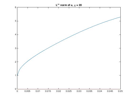
(a) $\chi=20$

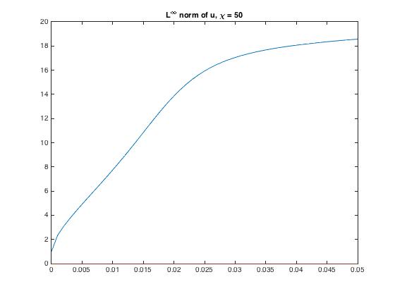
(b) $\chi=50$

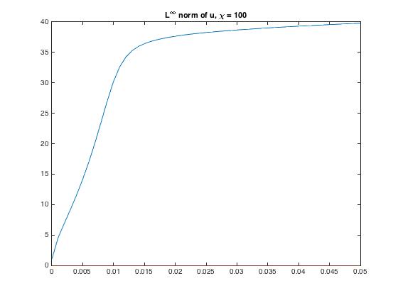
(c) $\chi=100$

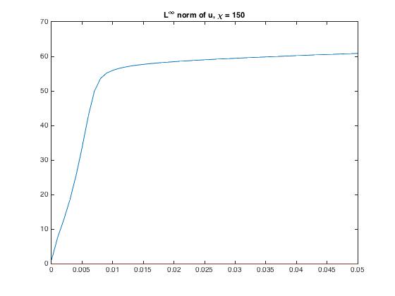
(d) $\chi=150$

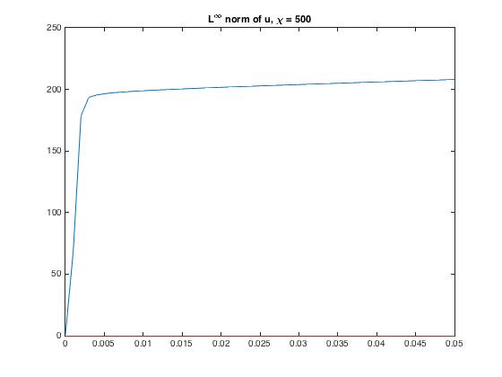
(e) $\chi=500$

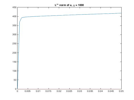
(f) $\chi=1000$

Figure 1: The evolution of the maximum concentration of criminal $\|u(\cdot,t)\|_{\infty}$ at a short time scale $t\in[0,.05]$ with initial condition given by $(u(x,0),v(x,0))=(e^{-x},e^{-x})$ and $B_{1}=B_{2}=1$.

On the other hand, at longer time scales (although not so long $t\in[0,5]$ with $\delta t=.05$) the dissipation dominates and in all cases we see eventual decay. This is illustrated in Figure 2, where we can see that by time $t=5$ the maximum density of criminals has reached a steady state.

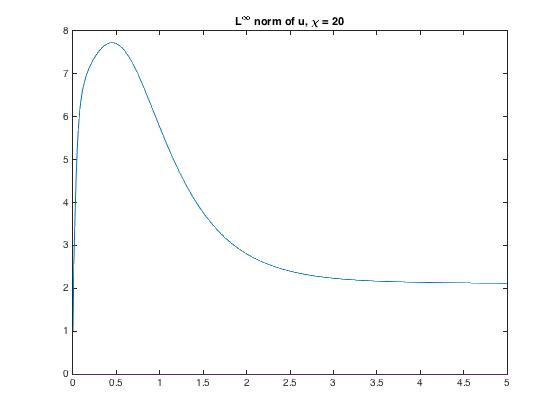
(a) $\chi=20$

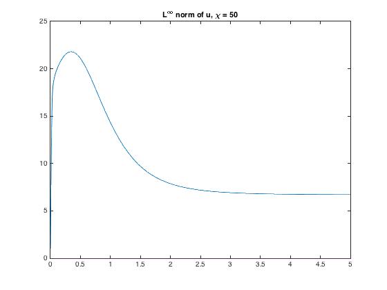
(b) $\chi=50$

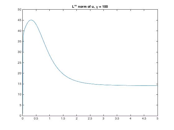
(c) $\chi=100$

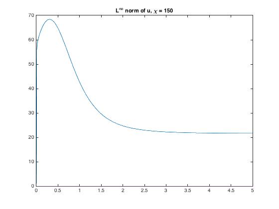
(d) $\chi=150$

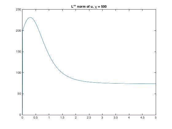
(e) $\chi=500$

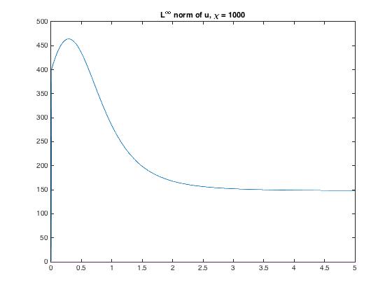
(f) $\chi=1000$

Figure 2: The evolution of the maximum concentration of criminal $\|u(\cdot,t)\|_{\infty}$ at a longer time scale ($t\in[0,5]$) with initial condition given by $(u(x,0),v(x,0))=(e^{-x},e^{-x})$ and $B_{1}=B_{2}=1$.

Another interesting thing to note that is that the steady-state of the maximum density of criminals increases with $\chi$. Thus, we do not see a relaxation to the constant steady states, which in this case are $u\equiv\frac{1}{2}$ and $v\equiv 2$. In fact, relaxation to the homogeneous steady-states occurs with $\chi$ small. However, as $\chi$ increases we observe to a non-constant hump-solution with the maximum at the origin. Figure 3

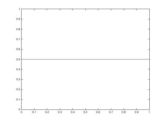
(a) $\chi=12$

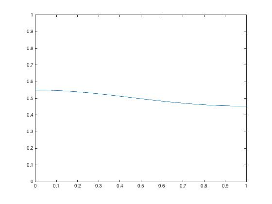
(b) $\chi=13$

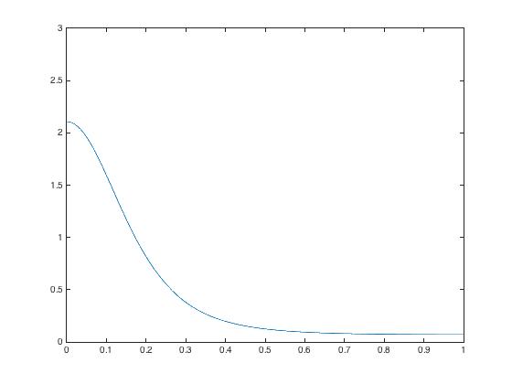
(c) $\chi=20$

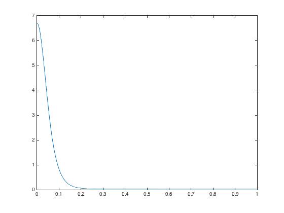
(d) $\chi=50$

Figure 3: Criminal density $u(x,t)$ at $t=20$ for various values of $\chi$.

7 Appendix: Two ODE lemmata

Let us separately formulate two auxiliary statements on boundedness and decay in linear ODIs with inhomogeneities enjoying certain averaged boundedness and decay properties.

Lemma 7.1

Let $T\in(0,\infty]$ and $\tau\in(0,T)$, and let $y\in C^{1}([0,T))$ and $h\in L^{1}_{loc}([0,\infty))$ be nonnegative and such that with some $a>0$ and $b>0$ we have

$$y^{\prime}(t)+ay(t)\leq h(t)\qquad\mbox{for all }t\in(0,T),$$

as well as

$$\frac{1}{\tau}\int_{t}^{t+\tau}h(s)ds\leq b\qquad\mbox{for all }t\in(0,T).$$

Then

$$y(t)\leq y(0)+\frac{b\tau}{1-e^{-a\tau}}\qquad\mbox{for all }t\in[0,T).$$

Proof.  This can be found e.g. in [47, Lemma 3.4]. $\Box$

Lemma 7.2

Let $y\in C^{1}([0,\infty))$ and $h\in L^{1}_{loc}([0,\infty))$ be nonnegative functions satisfying

$$y^{\prime}(t)+ay(t)\leq h(t)\qquad\mbox{for all }t>0$$

with some $a>0$. Then if

$$\int_{t}^{t+1}h(s)ds\to 0\qquad\mbox{as }t\to\infty,$$

we have

$$y(t)\to 0\qquad\mbox{as }t\to\infty.$$

Proof.  An elementary derivation of this has been given in [12, Lemma 4.6], for instance. $\Box$ Acknowledgement.  The second author acknowledges support of the Deutsche Forschungsgemeinschaft in the context of the project Emergence of structures and advantages in cross-diffusion systems (No.– 411007140, GZ: WI 3707/5-1). The first author was supported by the NSF Grant DMS-1516778.