Arrested dynamics of the dipolar hard-sphere model

Abstract

We report the combined results of molecular dynamics simulations and theoretical calculations concerning various dynamical arrest transitions in a model system representing a dipolar fluid, namely, $N$ (soft core) rigid spheres interacting through a truncated dipole-dipole potential. By exploring different regimes of concentration and temperature, we find three distinct scenarios for the slowing down of the dynamics of the translational and orientational degrees of freedom: At low ($\eta=0.2$) and intermediate ($\eta=0.4$) volume fractions, both dynamics are strongly coupled and become simultaneously arrested upon cooling. At high concentrations ($\eta\geq 0.6$), the translational dynamics shows the features of an ordinary glass transition, either by compressing or cooling down the system, but with the orientations remaining ergodic, thus indicating the existence of partially arrested states. In this density regime, but at lower temperatures, the relaxation of the orientational dynamics also freezes. The physical scenario provided by the simulations is discussed and compared against results obtained with the self-consistent generalized Langevin equation theory, and both provide a consistent description of the dynamical arrest transitions in the system. Our results are summarized in an arrested states diagram which qualitatively organizes the simulation data and provides a generic picture of the glass transitions of a dipolar fluid.

I Introduction

The substantial progress in the synthesis and fabrication of anisotropic colloids glotzer ; walther ; zhangt ; cayre , along with their unique ability for self-assembly and structural reconfiguration walther ; zhangt ; safran ; nych ; butter , provides a route for the design of new specialized materials with novel physical properties and with specific functionalities of high technological interest. Colloids of non-spherical shapes have long been known, but recognition that anisotropy in interactions constitutes another potential tool for engineering particular targeted structures has brought a widespread research enthusiasm in dipolar systems safran ; nych ; butter ; tlusty ; klokkenburg ; rovigatti ; cattes ; sindt ; koperwas ; weis ; belloni ; yethiraj . Even at thermodynamic equilibrium conditions and in the absence of external fields, dipolar suspensions tend to assemble into energetically favorable head-to-tail configurations and typically display a rich structural, dynamical and phase behavior arising from the complex and highly anisotropic nature of the dipolar interaction belloni ; cattes ; weis ; pincus ; blaak1 ; blaak2 ; goyal1 ; goyal2 ; goyal3 .

The current interest in structures of increasing complexity, however, has also triggered investigations of self-assembly under non-equilibrium conditions testard ; varrato ; kim ; stratford . Colloidal suspensions, in particular, have been observed to undergo distinct transitions to non-crystalline amorphous states. At high densities, for instance, they can form glassy states, where the main underlying physical mechanism for dynamical arrest is nearest-neighbor caging inhibiting individual motion pusey ; vanmegen . At low densities, they may also undergo gelation by increasing the mutual interactions among particles, prompting long-lived physical (reversible) bonding between particles, which thus facilitates the formation of percolated networks capable of sustaining weak mechanical stresses foffi ; zacarelli ; pastore ; sciozacca . Striking similarities, but also fundamental differences, have been highlighted between the microscopic dynamics and the mechanical response of both gels and glasses pastore ; zacarelli .

Dipolar colloids have been the subject of numerous investigations based on computer simulations rovigatti ; dijkstra ; rovigatti-PRL-2011 ; goyal1 ; goyal2 ; goyal3 ; blaak1 ; blaak2 . Goyal et al., for example, carried out molecular dynamics (MD) studies aimed at outlining the equilibrium phase diagram in the packing fraction ($\eta$) vs temperature ($T$) plane of monocomponent fluids of hard spheres (HS) with embedded dipoles goyal1 and of binary mixtures with difference in size and dipolar moment goyal2 ; goyal3 . One of the most interesting aspects of such diagrams is the observation that, besides different crystalline (e.g., fcc, hcp, bct), fluid, and string-fluid equilibrium phases, a region of percolated networks of crossed-links chains exists, occurring at intermediate temperatures and at nearly all the volume fractions considered, thus describing a region of gel-like states. In addition, Blaak et.al., blaak1 ; blaak2 demonstrated that, at low densities ($\eta<0.1$), a slight elongation of the particles into dumbbells favors branching of dipolar chains, and hence, space-spanning networking towards the gel state. It was also highlighted that this behavior is accompanied by a noteworthy slowing down of the translational dynamics, closely resembling well known features of physical (reversible) gelation in systems with short-ranged but spherically-symmetric depletion attractions sciozacca , just as it occurs in the case of colloid-polymer mixtures pham ; bergenholtz and systems with adhesive (sticky) interactions ramon1 ; ramon2 .

The theoretical modeling of the dynamical arrest of dipolar fluids is not abundant. Schilling and Scheidsteger schilling-PRE-1997 applied the mode coupling theory (MCT) of the glass transition (GT) to predict the existence of several dynamical arrest transitions in a dipolar HS fluid and outlined the corresponding non-equilibrium states diagram. More recently, the same essential features were also observed within the self-consistent generalized Langevin equation (SCGLE) theory Elizondo-PRE-2014 . To date, however, characterizations of the glassy and gel behavior of dipolar liquids, based on the simultaneous use of simulations and theoretical approaches, are rather scarce. Thus, it remains to be understood whether the competition between caging and bonding, along with the highly anisotropic character of the interactions (which couples translational and orientational motion) mediates the various dynamical arrest transitions. In particular, the role of the orientational dynamics in both the glass and gel transitions has not been fully determined.

A collection of $N$ rigid spheres of diameter $\sigma$ bearing a dipolar moment $\bm{\mu}$ is clearly one of the simplest representations of a dipolar fluid, a model that possesses a remarkable theoretical significance wertheim ; gray-molec-fluid-1984 , since it combines both spherical entropic and anisotropic energetic interactions. Notwithstanding its apparent conceptual simplicity, the distinct glassy behavior of such system is far from being completely understood. Hence, a main aim of this work is to report the results of extensive MD simulations carried out on a slightly simplified version of this model, introduced for practical convenience. We refer to a system of spherical particles whose repulsive-core interaction is given by the so-called Weeks-Chandler-Andersen (WCA) potential weeks-JCP-1971 . For simplicity, and in order to focus on the effect of anisotropy in the interactions, rather than on their long-range nature, the particles further interact by a truncated dipole-dipole potential. For this model, we have investigated different regimes of concentration and temperature where, on the basis of previous theoretical schilling-PRE-1997 ; Elizondo-PRE-2014 and simulation goyal1 ; goyal2 ; goyal3 ; blaak1 ; blaak2 results, various dynamical arrest transitions, including gels and glasses, are expected to occur.

Therefore, instead of considering equilibrium phases, in this contribution we are specifically interested in investigating those morphological transformations driven by conditions of dynamical arrest. In particular, we find three types of transitions: (i) the simultaneous arrest of the dynamics of both the translational (TDF) and orientational degrees of freedom (ODF), occurring at low and intermediate concentrations upon lowering the temperature; (ii) an ordinary GT for the translational dynamics, occurring at high densities and high-to-intermediate temperatures, but where the relaxation of the orientational dynamics remains ergodic; and (iii) the subsequent arrest of the ODF in a positionally frozen structure of particles, occurring also at high densities but lower temperatures. Our findings thus suggest the existence of at least three different GTs in the parameters space $(\eta,T^{*})$, which describe distinct microscopical underlying mechanisms for arrest.

Besides the analysis of the dynamics of the TDF, given in terms of observables such as the self-part of the Fourier transform of the van Hove correlation function and the mean square displacement, we also consider explicitly the dynamics of the ODF of the model towards the GT. This is described in terms of a proper set of orientationally sensitive correlation functions wertheim ; gray-molec-fluid-1984 ; schilling-PRE-1997 ; Elizondo-PRE-2014 and the corresponding angular mean square deviations. As we show below, this allows us to unravel important features of the dynamical arrest transitions of a dipolar fluid not fully described in previous investigations.

Finally, to provide a stronger physical insight, we complement the MD simulation results with a theoretical analysis based on the self-consistent generalized Langevin equation (SCGLE) theory Elizondo-PRE-2014 of dynamical arrest. We particularly focus on the study of the so-called non ergodicity parameters, describing the long-time dynamics of the fluid in the vicinity of each glass transition, and summarized in an arrested state diagram, which organizes qualitatively our results from simulations. The physical scenario emerging from the theory is in remarkable agreement with the features observed in the simulations, thus providing a consistent physical description of dynamical arrest.

This paper is organized as follows: in section II we define the model for the MD simulations and discuss the physical observables of interest along with the simulation details; in section III we present and discuss the MD simulation results; in section IV we complement these results with a theoretical discussion and show that they are consistent, which provides a comprehensive picture of the glassy behavior of the dipolar fluid. Finally, in section V we formulate our conclusions.

II Simulations: methodological aspects

The standard tools of MD cannot be directly applied to simulate a dipolar hard-sphere (DHS) fluid due to the mismatch between the discontinuous HS potential and the soft dipolar contribution. The former can be properly approached only via an event-driven algorithm alder-JCP-1959 ; lubachevsky-JCP-1991 , whereas the latter requires a continuous-time approach. One may use a Monte Carlo (MC) sampling considering both hard and soft potentials, but this only would be useful if our main purpose were the determination of the static properties. The absence of a well defined time variable in MC simulations, however, renders the evaluation of dynamical quantities complicated (MC time is nevertheless used some times, see, for instance, Ref. berthier-JPCM-2007 ). To circumvent these limitations, we have introduced a set of simplifying modifications to the pair interactions between dipolar spheres. Similarly, rather than simulating an exhaustive catalog of physical properties, here we shall focus on the dynamical properties associated with the (translational and rotational) Brownian motion and tracer diffusion properties, as explained in what follows.

II.1 Model system.

We have simulated a system of $N$ spherical particles in a volume $V$, with a pairwise potential of interaction between particles (labeled as $a$ and $b$) given by

$$U^{ab}({\bf r}_{a},\bm{\mu}_{a};{\bf r}_{b},\bm{\mu}_{b})=U_{\text{WCA}}^{ab}(|{\bf r}_{b}-{\bf r}_{a}|)+U_{\text{TD}}^{ab}({\bf r}_{b}-{\bf r}_{a},\bm{\mu}_{a},\bm{\mu}_{b}).$$ (1)

where ${\bf r}_{a}$ and ${\bf r}_{b}$ are the vectors describing the position of the center of mass of particles $a$ and $b$, respectively, and with $\bm{\mu}_{a}$ and $\bm{\mu}_{b}$ being their corresponding dipolar moments. The first term on the right side of Eq. (1) represents the hard-core interaction, and is given by the so-called Weeks-Chandler-Andersen (WCA) potential weeks-JCP-1971

$$U_{\text{WCA}}^{ab}(r_{ab}) = 4\epsilon_{\text{\tiny{WCA}}}^{ab}\left[\left(\frac{\sigma_{ab}}{r_{ab}}\right)^{12}-\left(\frac{\sigma_{ab}}{r_{ab}}\right)^{6}+\frac{1}{4}\right]\qquad\text{for}\;r_{ab}<2^{1/6}\sigma_{ab},$$ (2)

$$= 0\qquad\text{otherwise,}$$

where $r_{ab}\equiv|{\bf r}_{ab}|=|{\bf r}_{b}-{\bf r}_{a}|$ and the particles have sizes $\sigma_{a}$ and $\sigma_{b}$, taken from a distribution with an average $\sigma_{ave}=1$ (this last equality sets the length scale of the model) and we define $\sigma_{ab}=(\sigma_{a}+\sigma_{b})/2$. Since we want to study glassy behavior at different densities, we have considered an equimolar binary mixture using two sizes $\sigma_{1}=\sigma_{ave}+\Delta\sigma$ and $\sigma_{2}=\sigma_{ave}-\Delta\sigma$ The deviation in sizes has been set to $\Delta\sigma=1/6$, which thus gives a ratio $\sigma_{1}/\sigma_{2}=1.4$, a common size ratio used to avoid crystallization in dense HS fluids berthier-PRE-2009 .

The second term on the right side of Eq. (1) represents the anistropic dipolar contribution to the interaction. In order to avoid all the complexities inherent to the specialized treatment of long-ranged ($\sim 1/r^{3}$) interactions allen-tildesley , we have considered a truncated dipolar potential which may be written as

$$U_{\text{TD}}^{ab}({\bf r}_{ab},\hat{\bm{\mu}}_{a},\hat{\bm{\mu}}_{b}) = \epsilon_{\text{\tiny{DIP}}}^{ab}\left[\frac{1}{r_{ab}^{3}}-\frac{1}{R^{3}}+3\frac{r_{ab}-R}{R^{4}}\right]\times$$ (3)

$$\left[\hat{\bm{\mu}}_{a}\cdot\hat{\bm{\mu}}_{b}-3(\hat{\bm{\mu}}_{a}\cdot\hat{\bf r}_{ab})(\hat{\bm{\mu}}_{b}\cdot\hat{\bf r}_{ab})\right]\qquad\text{for}\;r_{ab}<R,$$

$$= 0\qquad\text{otherwise}.$$

Here ${\bf\hat{r}}_{ab}={\bf r}_{ab}/r_{ab}$, $\hat{\bm{\mu}}_{a}\equiv\bm{\mu}_{a}/\mu_{a}$, $R$ is a cut-off distance for the dipolar interaction and $\epsilon_{DIP}^{ab}=\mu_{a}\mu_{b}$. In this work we are setting $R=3\sigma_{ave}$. The magnitude of a given dipole moment is proportional to its diameter to the power $3/2$, that is, $\mu_{i}=\mu_{0}(\sigma_{i}/\sigma_{ave})^{3/2}$ ($i=1,2$), where $\mu_{0}$ is a common dipole scale taken here as $\mu_{0}=1$. The reason to introduce this dependence is to keep the interaction at contact (i.e., for $r_{ab}\approx\sigma_{ab}$) approximately the same for all contacts, be they between large dipoles, small dipoles, or a small dipole with a large one; otherwise the attraction at contact between small dipoles is substantially larger than the one between large dipoles, and segregation phenomena may appear. For simplicity all dipoles are assumed to have mass $m=1$ (this sets the mass scale) and moment of inertia $I=1/10$, and the scale of the WCA potential is set by $\epsilon_{\text{\tiny{WCA}}}^{ab}=1$ for all $a,b=1,2$, fixing in this way both energy and time scales.

II.2 Physical observables.

In this contribution we focus on the single particle dynamics, which is sampled with better statistics than collective dynamics. Specifically, we consider the self-part of the generalized intermediate scattering functions (ISFs) and mean square deviations defined below as a measure of translational and rotational diffusion. To monitor the stability of the simulations, we have also checked translational and rotational kinetic energies, potential energies, and pressure.

Also reviewed, and of special interest, are those quantities that may signal a breakdown of the homogeneity or the isotropy of the fluid. To test for possible crystallization, we have used the $q_{4},q_{6},Q_{4}$ and $Q_{6}$ orientational order parameters defined by Steinhardt and Nelson steinhardt-PRB-1983 ; tenvolde-JCP-1996 . To look for possible segregation, instead, we introduce a simple ”sameness” parameter, which measures how many dipoles of the same size are within a cut-off distance of any given dipole, compared to how many dipoles of the other size can be found. More concretely, this is defined for the $a$-th dipole as $S_{a}=\sum_{\langle nn\;a\rangle}z_{ab}/N_{\langle nn\;a\rangle}$, where we take $z_{ab}=1$ if dipoles $a$ and $b$ are of the same size, and $z_{ab}=-1$ otherwise. Here the sum is taken over all nearest neighbors (nn) to $a$, as defined by the cut-off distance, and $N_{\langle nn\;a\rangle}$ is the number of those nearest neighbors. It is also quite important to check the variance in $S$, since a small value for this variance indicates some degree of ordering. The cutoff distance used here is the same one used for the aforementioned Steinhard-Nelson order parameters, and has been taken for our purposes as the distance for the first minimum in the pair distribution function, $g(r)$, which is larger than $\sigma_{1}$. Finally, we also monitor the total magnetization, ${\bf M}=\sum_{a}^{N}\bm{\mu}_{a}/N$, so we can rule out any long range orientation of the dipoles. In all the states considered below $\langle{\bf M}\rangle\approx\mathbf{0}$, and no crystallization or particle segregation occurs.

Let us now discuss the mean squared deviations. For the TDF, the common definition of the mean squared displacement (MSD) is used,

$$W_{T}(t)=\frac{1}{N}\langle\sum_{a}[{\bf r}_{a}(t)-{\bf r}_{a}(0)]^{2}\rangle,$$ (4)

from which one can obtain a diffusion coefficient using the well known long-time limit (Einstein’s relation) $W_{T}(t)=6D_{T}t$.

The description of rotational diffusion is slightly more complex. Recall that in our case, the ODF are described by the set $\{\hat{\bm{\mu}}_{1}(t),\hat{\bm{\mu}}_{2}(t),...,\hat{\bm{\mu}}_{N}(t)\}\in\mathbb{U}^{3}$, where each of the vectors $\hat{\bm{\mu}}_{a}(t)$ describe a point over the unit sphere $\mathbb{U}^{3}$. As it is immediately apparent, the long-time limit of the diffusion of such points over a spherical surface is a static homogeneous covering, which gives a $W_{R}(t)$ that saturates to a constant after a sufficiently long time castro . There have been various efforts to define different ways of measuring diffusion over a spherical surface. In particular, there is a method that generates a vector $\Delta\vec{\phi}(t)$ tangential to the surface and normal to the direction of displacement, and with the magnitude of the traversed angle. One then concatenates these vectorial increments to obtain a total displacement vector $\vec{\phi}(t)$ mazza-PRE-2007 . This measure of diffusion does not saturate and, for small angular increments $\Delta\phi$, gives a linear behavior in the long time limit, i.e., $W_{\bm{\phi}}(t)=4D_{\phi}t$. However, since the $\Delta\vec{\phi}$ contributions are all tangential to the surface of the sphere, their sum $\vec{\phi}$ drifts away from the surface for any finite displacements, and thus, ends up predicting normal diffusion even in cases where there is clear arrest and where the dipoles cannot deviate more than a small fraction of $\pi$ from its original orientation. We therefore stick with a measure of rotational diffusion that saturates and identify arrest as those cases where a rotational MSD does not reach (or takes an exceedingly long time to reach) its saturation value. Specifically, we have considered the mean square deviations (see appendix A)

$$W_{\theta}(t)\equiv\frac{1}{N}\left\langle\sum_{a}[\Delta\theta_{a}(t)]^{2}\right\rangle,$$ (5)

and

$$W_{\sin{\theta}}(t)\equiv\frac{1}{N}\left\langle\sum_{a}[\sin{\Delta\theta_{a}(t)}]^{2}\right\rangle$$ (6)

with $\Delta\theta_{a}(t)\equiv\theta_{a}(t)-\theta_{a}(0)$. In general, the results found for $W_{\theta}(t)$ and $W_{\sin\theta}(t)$ are quite similar and provide the same information. Therefore we will be reporting from now on only the results for $W_{\theta}(t)$. The observable $W_{\sin\theta}(t)$, however, is important because it allows to develop a closed formula to obtain the rotational diffusion coefficient from simulations (see Eqs. (5) and (6) of appendix A)

With respect to the correlation functions, there is a common approach which, for completeness, is briefly reviewed here. Details are carefully discussed in Refs. gray-molec-fluid-1984 ; schilling-PRE-1997 ; Elizondo-PRE-2014 . One starts by considering a microscopical density of particles at position ${\bf r}$ and orientation $\hat{\bm{\mu}}$, at time $t$, defined by

$$\rho({\bf r},\hat{\bm{\mu}};t)=\frac{1}{\sqrt{N}}\sum_{a}\delta({\bf r}-{\bf r}_{a}(t))\delta(\hat{\bm{\mu}}-\hat{\bm{\mu}}_{a}(t)).$$ (7)

Instead of constructing a generalized van Hove function with variables ${\bf r}$, $\hat{\bm{\mu}}$ at time $t=0$, and ${\bf r}^{\prime}$, $\hat{\bm{\mu}}^{\prime}$ at time $t$, it is customary to consider first the Fourier transform and spherical harmonics expansion of $\rho({\bf r},\hat{\bm{\mu}};t)$ gray-molec-fluid-1984 , commonly referred to as tensorial density modes, and given by

$$\hat{\rho}_{lm}({\bf k},t) = \sqrt{4\pi}i^{l}\int_{V}d^{3}{\bf r}\,e^{i{\bf k}\cdot{\bf r}}\int d^{2}\bm{\mu}\,Y_{lm}^{*}(\hat{\bm{\mu}})\,\rho({\bf r},\hat{\bm{\mu}},t),$$ (8)

$$= \sqrt{\frac{4\pi}{N}}i^{l}\sum_{a}e^{i{\bf k}\cdot{\bf r}_{a}(t)}\,Y^{*}_{lm}(\hat{\bm{\mu}}_{a}(t)),$$

where $Y_{lm}(\hat{\bm{\mu}})$ are spherical harmonics and k is the scattering vector. From here, the fundamental correlators are defined by a family of intermediate scattering functions (ISFs) of the form schilling-PRE-1997 ; Elizondo-PRE-2014

$$F_{lm,l^{\prime}m^{\prime}}({\bf k},{\bf k}^{\prime},t) = \left\langle\hat{\rho}_{lm}({\bf k},0)\,\hat{\rho}^{*}_{l^{\prime}m^{\prime}}({\bf k}^{\prime},t)\right\rangle$$ (9)

$$= \frac{4\pi}{N}i^{l^{\prime}-l}\sum_{ab}\left\langle e^{i[{\bf k}\cdot{\bf r}_{a}(0)-{\bf k}^{\prime}\cdot{\bf r}_{b}(t)]}\,Y^{*}_{lm}(\hat{\bm{\mu}}_{a}(0))\,Y_{l^{\prime}m^{\prime}}(\hat{\bm{\mu}}_{b}(t))\right\rangle.$$

Up to now no assumptions have been made about the fluid. However, one knows that in an homogeneous system, a van Hove correlation function does not depend on two vectors ${\bf r}$ and ${\bf r}^{\prime}$ separately, but only on the displacement ${|\bf r}-{\bf r}^{\prime}|$. As a result, the corresponding ISFs will only depend on one wavevector ${\bf k}$, instead of the two appearing, for instance, in eq. (9). Furthermore, in an isotropic system the van Hove function does not depend on the two full sets of angles defining the orientations $\hat{\bm{\mu}}$ and $\hat{\bm{\mu}^{\prime}}$, but only on three angular variables gray-molec-fluid-1984 . Following the form of the anisotropic dipolar interaction, an appealing choice is to use the projections of $\hat{\bm{\mu}}$ and $\hat{\bm{\mu}^{\prime}}$ over the line connecting the two dipoles (assuming some orientation for this line which, at the end, results irrelevant), and the dihedral angle between them. This is equivalent to choosing the line between the two particles as the ${\bf\hat{z}}$ axis, a prescription known as the $k$-frame choice wertheim ; gray-molec-fluid-1984 (also referred to as interaction frame). Going again into Fourier space, the equivalent procedure is to rotate the coordinate system so that the wavevector ${\bf k}$ points in the direction of the the ${\bf\hat{z}}$ axis.

As discussed in Ref. schilling-PRE-1997 , for an isotropic space and using well-known properties of spherical harmonics, this choice imposes several restrictions on $F_{lm,l^{\prime}m^{\prime}}$. The most important of them being that, for a nonzero correlator, one only needs to consider $m=m^{\prime}$. In this way, one gets a right counting of variables, since the ISF now uses just three orientational indices. We are then left with correlators of the form

$$F_{ll^{\prime}\,m}(k\hat{\bf z},t)=\frac{4\pi}{N}i^{l^{\prime}-l}\sum_{ab}<e^{ik[z_{a}(0)-z_{b}(t)]}\,Y^{*}_{lm}(\hat{\bm{\mu}}_{a}(0))\,Y_{l^{\prime}m}(\hat{\bm{\mu}}_{b}(t))>.$$ (10)

Finally, and as indicated before, in this contribution we are interested only in the self part of these correlation functions, that is, the correlators of the positions and orientations of a single particle,

$$F^{\text{S}}_{ll^{\prime}\,m}(k\hat{\bf z},t)=\frac{4\pi}{N}i^{l-l^{\prime}}\sum_{a}<e^{ik[z_{a}(0)-z_{a}(t)]}\,Y^{*}_{lm}(\hat{\bm{\mu}}_{a}(0))\,Y_{l^{\prime}m}(\hat{\bm{\mu}}_{a}(t))>.$$ (11)

There are additional restrictions for $F_{ll^{\prime}\,m}(k{\bf\hat{z}},t)$ schilling-PRE-1997 . Two of them are worth mentioning here: (i) these correlation functions are zero unless $l-l^{\prime}$ is even, and (ii), $F_{ll^{\prime}\,m}$ is zero at time $t=0$ unless $l^{\prime}=l$.

II.3 Molecular Dynamics simulations

We have considered a Newtonian MD that uses the velocity-Verlet integrator, for both translations and rotations. Both sets of degrees of freedom are coupled to stochastic thermostats that performs velocity re-scaling in the same spirit as the Bussi-Donadio-Parrinello thermostat bussi-JCP-2007 . Two thermostats are used because, in general, the evolution timescales for translations and rotations are different, and the system tends to show a difference in temperatures analogous to the Hot-Solvent/Cold-Solute problem that is pervasive in other applications of MD, when some type of velocity rescaling is used with only one thermostat cheng-JPC-1996 .

We have simulated a total of $N$ dipolar particles ($N_{1}=N_{2}=N/2$) in a cubic box of volume $V$, with periodic boundary conditions. The effective packing fraction, $\eta=N\pi(\sigma_{1}^{3}+\sigma_{2}^{3})/12V$, and the scaled temperature, $T^{*}$, were used to explore different points in the $(\eta,T^{*})$ plane. Specifically, we have investigated state points along four different Paths. Three of them consist in fixing the volume fraction to the values $\eta=0.2$ (Path 1), $0.4$ (Path 2) and $0.6$ (Path 3), and varying the temperature in the range $0.2\leq T^{*}\leq 2$. In addition, we also considered the isotherm $T^{*}=1$ and varied the concentration as $0.2\leq\eta\leq 0.7$ (Path 4). In all cases, we have considered $N_{1}=N_{2}=4096$ for a total of $8192$ particles, a number large enough so we have not detected any changes in the behavior of the fluid when halving $N$. For each state point investigated, $8$ different seeds (realizations) of the system have been used to explore the available phase space and to improve statistics. The time increment for $T^{*}=1$ was set to $dt_{1}=5\times 10^{-4}$, and for other temperatures we use $dt=dt_{1}/\sqrt{T^{*}}$. The computing of the self ISFs has been carried out performing, for each configuration considered, the sum indicated in Eq. (11) taking as the vertical direction each of the three coordinate axes, that is, using the original coordinates and then performing the two cyclic rotations $xyz\to zxy\to yzx$. These correlators are real when we consider both possible orientations for the ${\bf z}$ axis. We start from a random, non-overlapping configuration, and then run a transient long enough to render stable values for the pressure and the potential energy of the system

III Simulation results

We now present the results of the described simulations, regarding the dynamical properties associated with the translational and rotational degrees of freedom.

III.1 Translational dynamics

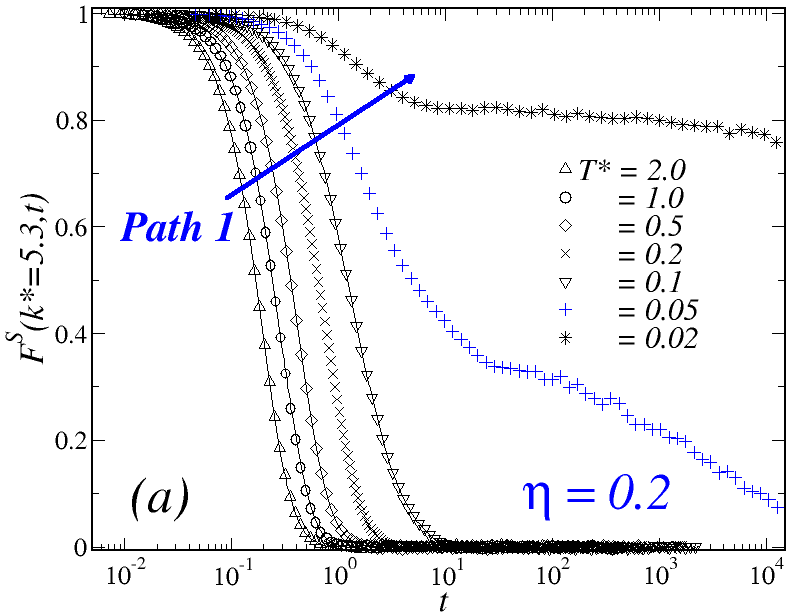
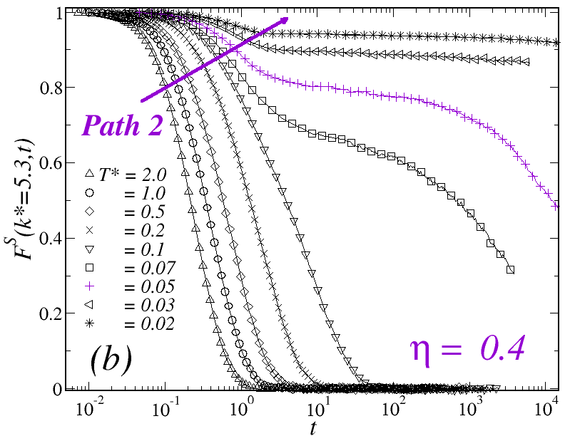
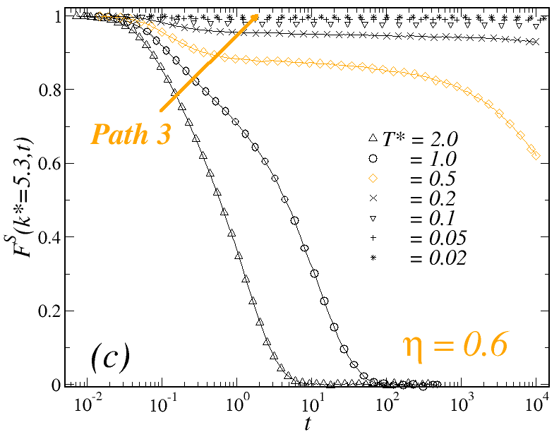
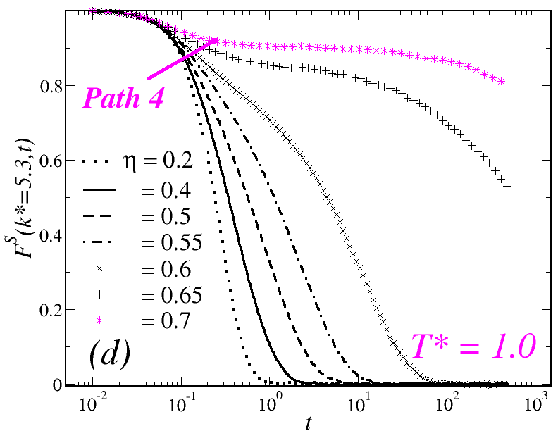
Figure 1: (Color online) Time evolution of the positional-density self correlation function, $F^{S}(k^{*}=5.3,t)$, with $k^{*}\equiv k\sigma_{ave}$, at three different concentrations: (a) $\eta=0.2$, (b) $\eta=0.4$, and (c) $\eta=0.6$, for different temperatures (as indicated); and at fixed temperature (d) $T^{*}=1.0$ and varying the concentration (as indicated). From left to right, the solid arrows intersect the curves in order of decreasing temperature (a-c) or increasing density (d).

To study the dynamics of the TDF of the model we considered the purely translational self-ISF, $F_{000}^{S}(k,t)\equiv F^{S}(k,t)$, and the MSD, $W_{T}(t)$. As indicated above, both observables were investigated at different state points of the $(\eta,T^{*})$ parameters space, organized for clarity in four Paths that approach dynamical arrest in different ways. In Fig.1, we summarize the results obtained for $F^{S}(k^{*}=5.3,t)$, with $k^{*}\equiv k\sigma_{ave}$, at the three isochores corresponding to (a) $\eta=0.2$, (b) $\eta=0.4$ and (c) $\eta=0.6$, and along the isotherm (d) $T^{*}=1$.

At the lowest density and high temperatures considered, the system’s behavior resembles that of a dilute HS gas (see also appendix B). Lowering $T^{*}$ at fixed $\eta$ (i.e. following the solid arrow of Fig.1 (a) from left to right, Path 1), a gradual slowing down in the relaxation dynamics is observed. Specifically at $T^{*}=0.05$, $F^{S}$ shows an inflection point and a stretched relaxation which remains finite over the time-scale of the simulations. Slightly below, at $T^{*}=0.02$, the arrest of the dynamics of the TDF becomes more noticeable with the emergence of a high plateau, which remains practically constant up to three decades in time.

Upon increasing the concentration to $\eta=0.4$ (Fig.1 (b), Path 2) one finds similar features. Within the range $0.1\leq T^{*}\leq 2$, $F^{S}$ becomes only moderately slower with respect to the previous case at comparable temperatures. At lower values, the self-ISF develops a second decay mode and the relaxation-time increases dramatically with small variations in $T^{*}$. A transient plateau appears at $T^{*}=0.05$, where this correlation function barely changes along three decades and remains finite at the longest time of the simulation. The height of this plateau, however, is noticeably larger in comparison to that found along the isochore $\eta=0.2$ at the same temperature. This suggests that the state point ($\eta=0.4,T^{*}=0.05$) is closer to conditions of dynamical arrest than ($\eta=0.2,T^{*}=0.05$). In addition, the appearance of a higher plateaus is typically associated to the formation of a mechanically stronger glassy state. It is worth stressing that, despite the small differences in the dynamics of the TDF along Paths 1 and $2$, a concomitant change in the structure of the system is also observed upon increasing $\eta$ from $0.2$ to $0.4$. These effects can be represented, for instance, by the evolution of the radial distribution function $g(r)$ along both isochores (see appendix B). In this work, however, we specifically focus in the analysis of the slow dynamics towards the GT.

For the isochore $\eta=0.6$ (Fig.1 (c), Path 3), $F^{S}$ becomes arrested and develops a high plateau at $T^{*}=0.5$ (and below). This value in temperature is relatively larger in comparison to those found along the two previous cases (roughly, one order of magnitude) and accounts for the strong influence of crowding in the dynamical arrest of the translational dynamics. These effects can be also emphasized by considering the results along the isotherm $T^{*}=1$ (Fig.1 (d), Path 4), where the features of a HS (i.e., density-driven) GT are displayed. In this case, the slowing down of the relaxation dynamics is observed for concentrations $\eta\geq 0.6$, where $F^{S}$ develops a two-steps relaxation pattern and eventually a non-decaying plateau at $\eta=0.7$. Therefore, the results along Paths 3 and $4$ support the interpretation that the critical temperature for the arrest of the translational dynamics represents a rapidly increasing function of $\eta$ at high densities.

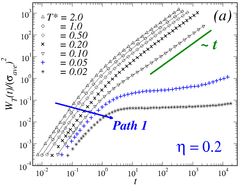
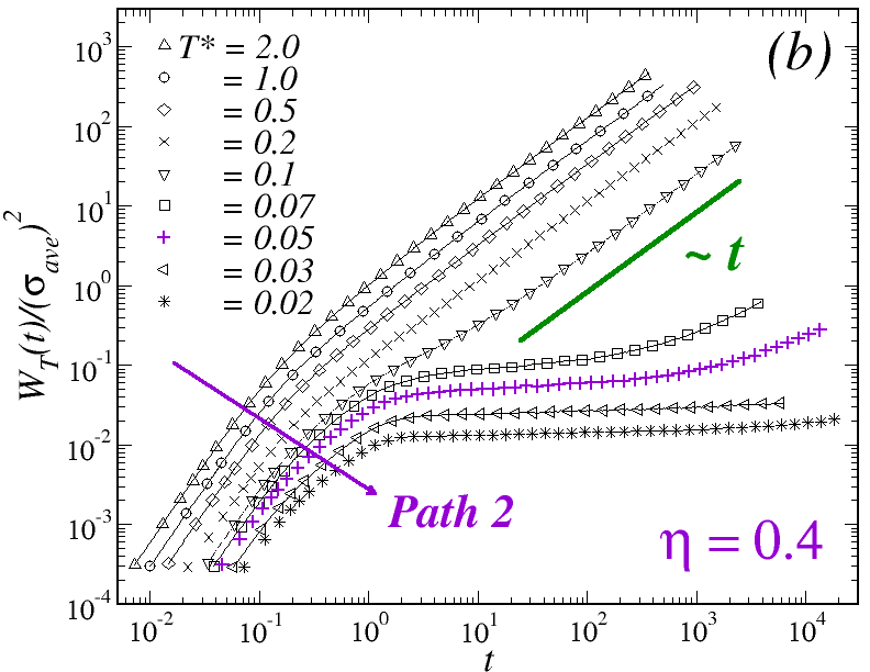
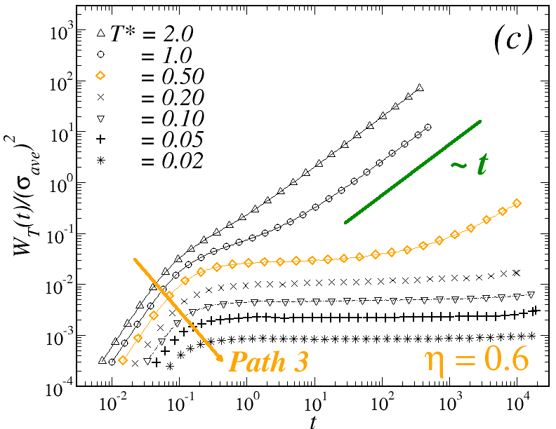
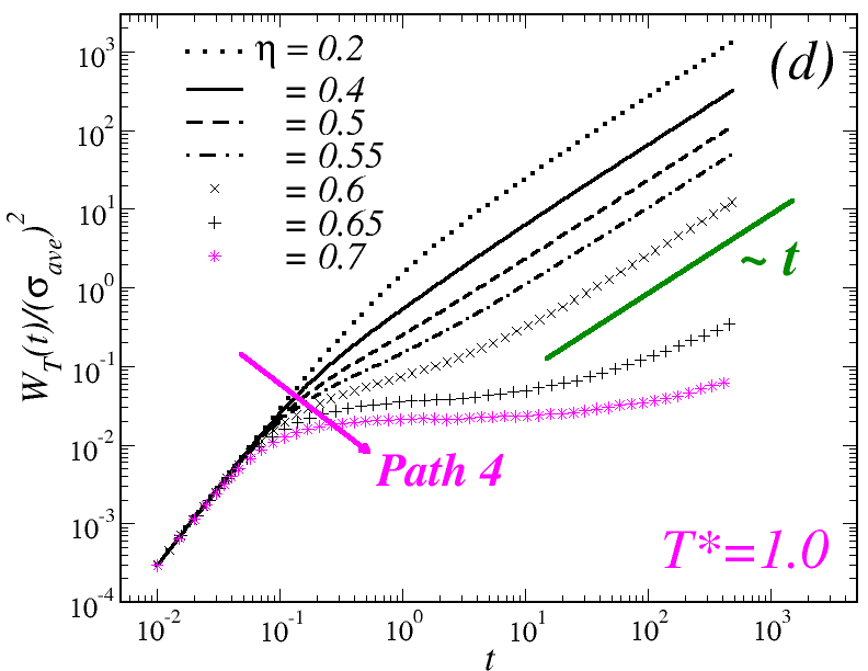
Figure 2: (Color online) Mean square displacements, $W^{*}(t)$ (in units of $\sigma_{ave}^{2}$), corresponding to the isochores: (a) $\eta=0.2$, (b) $\eta=0.4$, and (c) $\eta=0.6$ and the same temperatures as in Fig.1; and for the isotherm (d) $T^{*}=1.0$. From left to right, the solid black arrows intersect the curves in order of decreasing temperature or increasing density. The (green) solid lines are a guide to the eye.

Besides the information provided by the self-ISF, one can also consider the evolution of the MSD, $W_{T}(t)$, along Paths 1-4. Both quantities are connected in the low-wave-vector, but the MSD represents an easily interpreted observable quantifying particle mobility and long-ranged transport. The corresponding data are displayed in Fig. 2 and consistently describe the physical scenario outlined by $F^{S}$. Along the isochores $\eta=0.2$ and $\eta=0.4$ (Figs. 2(a) and 2 (b), respectively), $W_{T}(t)$ undergoes the typical evolution from ballistic ($\sim t^{2}$) to diffusive ($\sim t$) behavior for $0.1\leq T^{*}\leq 2$. At lower temperatures, the particles cease to diffuse and the MSD develops transient plateaus followed by the emergence of a small subdiffusive regime for longer times. In both Paths, this is observed to occur at $T^{*}\approx 0.05$, and flat plateaus extending the observation time of the simulation appear for lower temperature.

As it might be expected from the results for $F^{S}$ along Path 3, the MSD shows arrest at $T^{*}=0.5$ for the isochore $\eta=0.6$ (Fig. 2(c)). Similarly, in the case of the isotherm $T^{*}=1$, $W_{T}(t)$ shows a slowing down with increasing density and develops plateaus for $\eta\geq 0.65$. This confirms that $F^{S}$ and $W(t)$ provide the same physical scenario regarding the dynamical arrest of the TDF.

To estimate the maximum possible displacement of the particles approaching to conditions of dynamical arrest, one can use the long-time value of the MSD. In the case of dense systems described by steep repulsive potentials, the square-root of this value is commonly referred to as the localization length, $l$, and represents a measurement of the local confinement, since it provides the displacement inside nearest neighbors cages. The quantity $l(\eta,T^{*})\equiv\sqrt{W_{T}(\eta,T^{*};t^{*}=10^{2})}$, for instance, shows that the particles only become slightly more localized upon increasing $\eta$ from $0.2$ to $0.4$, despite the dynamical (and structural) differences found along Paths 1 and $2$ (i.e., $l(\eta=0.2,T^{*}=0.05)\approx l(\eta=0.4,T^{*}=0.05)$). In addition, both $l(\eta=0.6,T^{*}=0.5)$ and $l(\eta=0.7,T^{*}=1)$ provide essentially the same value, $l\approx 0.1\sigma_{ave}$, which corresponds to a cage size of approximately $10\%$ of the characteristic diameter, a typical feature of a HS glass.

In summary, the results for $F^{S}(k^{*},t)$ and $W_{T}(t)$ outline the main features of arrested dynamics of the TDF of the simulated model. At low and intermediate concentrations, the dynamics freezes at nearly the same temperature and shows essentially the same localization length for the constitutive particles, but with some differences in the corresponding relaxation times, decay patterns, and also at the structural level. The results for the high density regime, instead, show that the critical temperature for dynamical arrest behaves as a monotonically and rapidly increasing function of the concentration, and that the dynamics of the TDF undergo a GT in the fashion of a HS system.

III.2 Orientational dynamics

We now turn our discussion to the dynamics of the ODF. For this, we have considered a set of orientationally sensitive correlation functions, $F^{S}_{ll^{\prime}m}(k,t)$, with $l=l^{\prime}>0$ and defined by Eq. (11); and the angular mean squared deviations, $W_{\theta}(t)$ and $W_{\sin\theta}(t)$, given by Eqs. (5) and (6). For simplicity, we will restrict ourselves to the analysis of ISFs of rank: $1\leq l=l^{\prime}\leq 2$. Furthermore, we have found that both $F_{221}^{S}$ and $F_{222}^{S}$ provide essentially the same information as $F_{220}^{S}$. Therefore, we specifically focus on the analysis of the correlation functions $F_{110}^{S}(k,t)$, $F_{111}^{S}(k,t)$, and $F_{220}^{S}(k,t)$. As mentioned before, a similar behavior is encountered for $W_{\theta}(t)$ and $W_{\sin\theta}(t)$, so we only report the former.

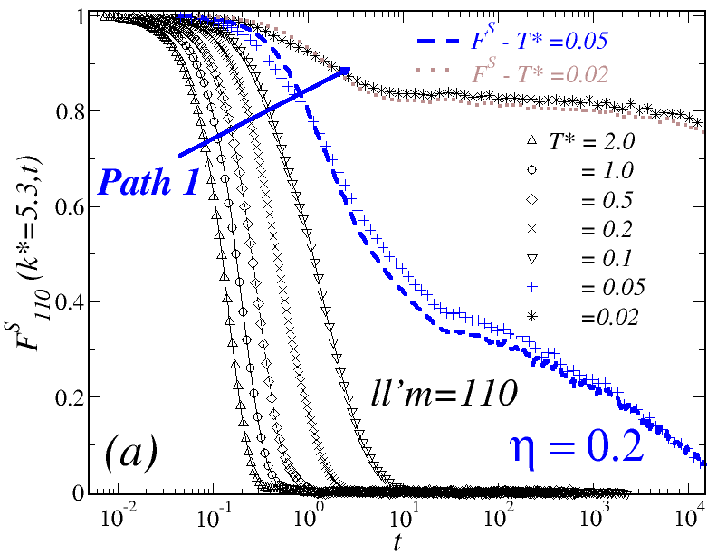
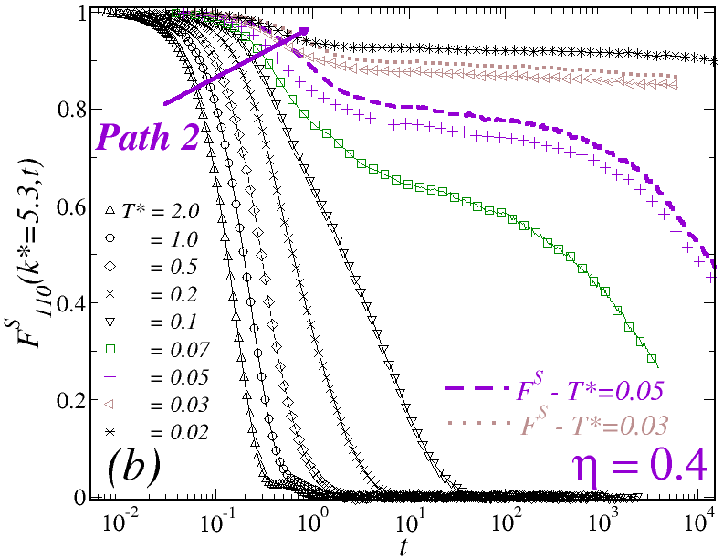
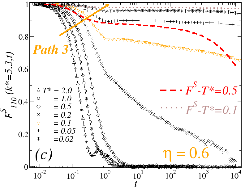
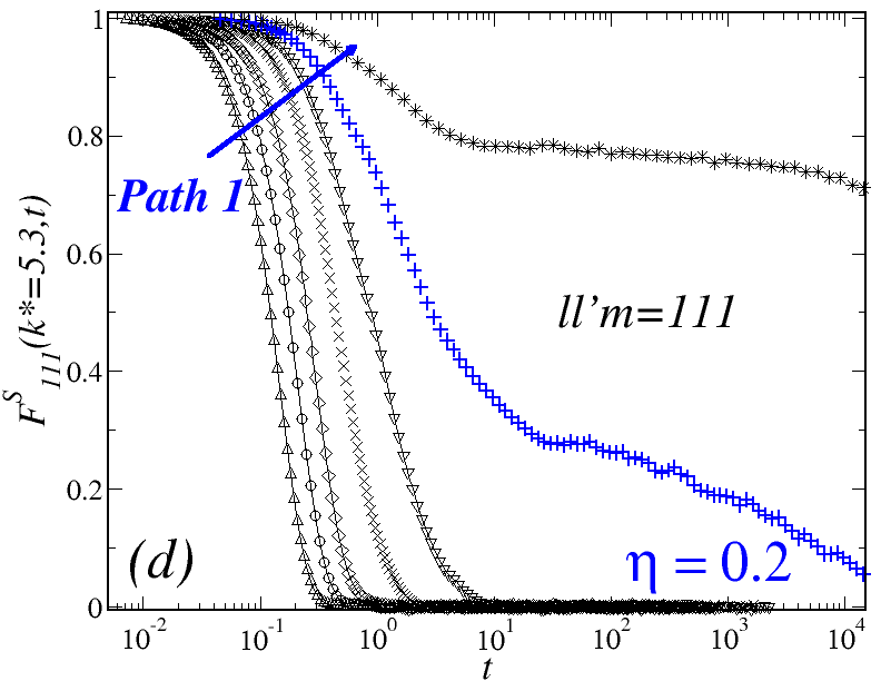
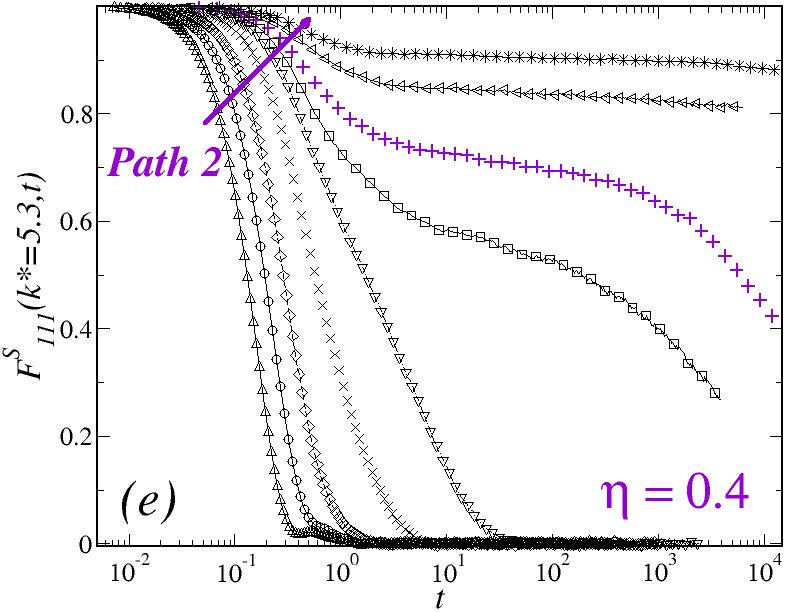
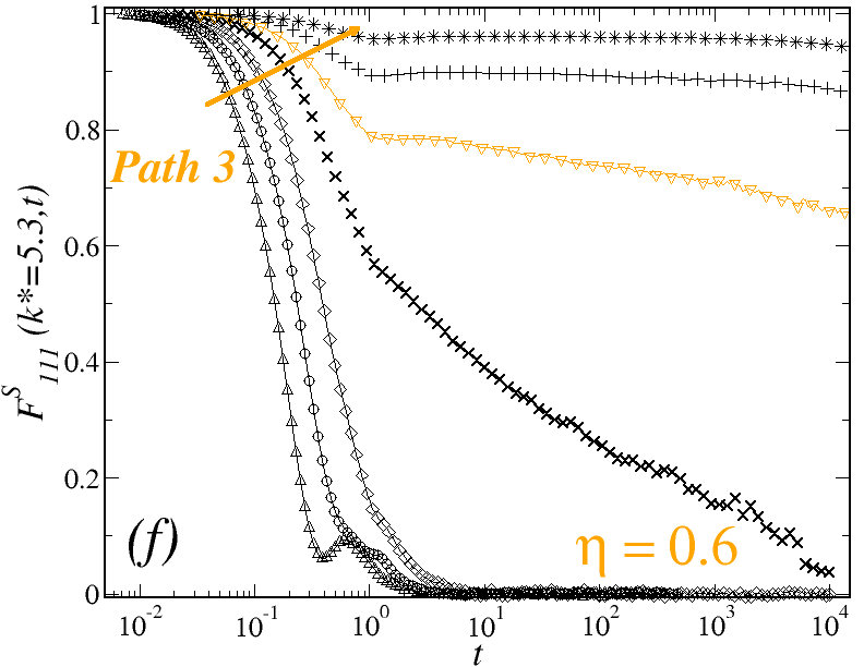
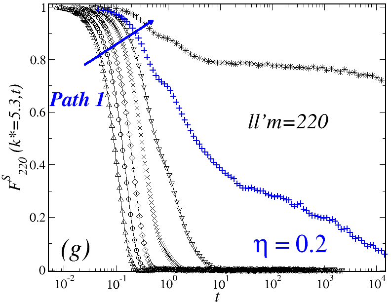
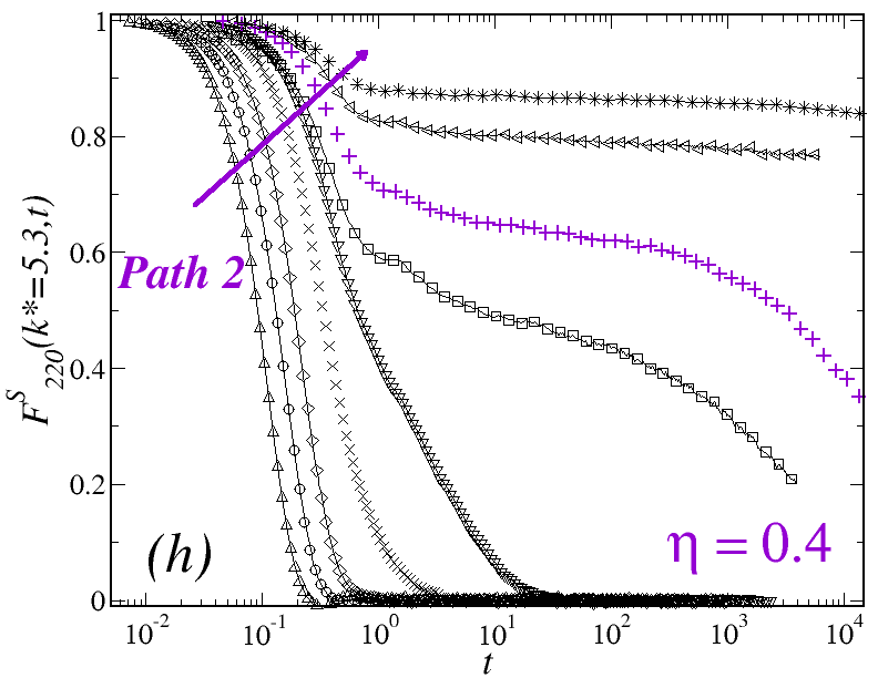
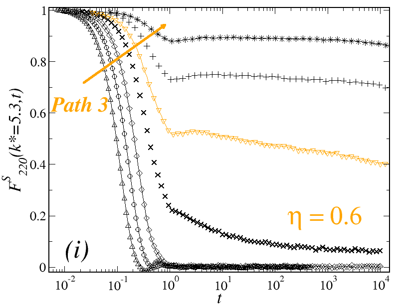
Figure 3: (Color online) Time evolution of the correlation functions $F_{110}(k^{*},t),F_{111}(k^{*},t)$ and $F_{220}(k^{*},t)$, evaluated at $k^{*}=5.3$, at three different concentrations $\eta=0.2$ (a)-(d)-(g), $\eta=0.4$ (b)-(e)-(h), $\eta=0.6$ (c)-(f)-(i), and at different temperatures (as indicated). For reference, the dashed and dotted lines in (a)-(b)-(c) illustrate the arrested behavior of $F^{S}(k,t)$ previously shown in Fig.1.

The results for the orientational ISFs along the three isochores previously considered (Paths 1,2,3), evaluated at $k^{*}=7$, are summarized in Fig.3. Either at low (first column, Figs. 3(a)-(d)-(g)) or intermediate concentration (middle column, Figs. 3(b)-(e)-(h)), $F_{110}^{S}$, $F_{111}^{S}$, and $F_{220}^{S}$ display essentially the same relaxation patterns and become gradually slower with decreasing temperature. Remarkably, all the correlation functions also follow the same trends of $F^{S}$ along Paths 1 and $2$, including their eventual arrest at $T^{*}=0.05$ (for clarity, the arrested behavior of $F^{S}$ is displayed again in Figs. 3(a)-(b)-(c) as the dashed and dotted lines). These features indicate a strong coupling in the dynamics of the TDF and ODF, thus evidencing their simultaneous arrest upon cooling.

This is to be contrasted with the scenario observed for $\eta=0.6$ (right column in Fig. 3). First, let us notice that the orientational ISFs remain ergodic (i.e., decay to zero) at $T^{*}=0.5$ (open diamonds in Figs.3 (c)-(f)- (i)), whilst $F^{S}$ undergoes dynamical arrest (red dashed line of Fig.3(c)). Lowering the temperature to $T^{*}=0.2$, $F^{S}_{110}$ and $F^{S}_{111}$ develop transient plateaus, which seem to decay slowly to zero in the time scale of the simulations, whereas $F^{S}_{220}$ develops a slightly different relaxation pattern characterized by a fast initial decay and followed by a stretched relaxation. These features indicate the existence of a transition to partially arrested states for the fluid, where the dynamics of the TDF undergoes a GT whereas the ODF remain ergodic. Furthermore, at $T^{*}=0.1$ the three correlation functions also become arrested, indicating another type of transition where the ODF may undergo a GT starting from a partially arrested state. Notice that this transition for the ODF occurs at a slightly higher temperature with respect to Paths 1 and $2$.

The existence of partially arrested states is also illustrated by the results shown in Fig. 4 for the orientational ISFs along the isotherm $T^{*}=1$, where the three correlation functions remain ergodic and practically unaffected by increasing the concentration up to $\eta=0.7$. This is in clear contrast with the behavior of $F^{S}$, which hardly relaxes to zero for $\eta=0.65$ and becomes arrested at $\eta\geq 0.7$, as already shown in Fig. 1 (d).

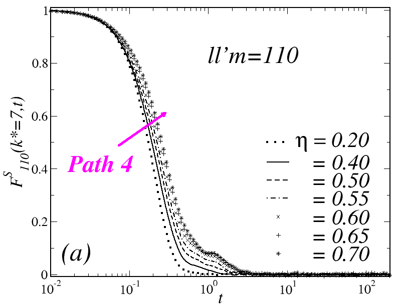
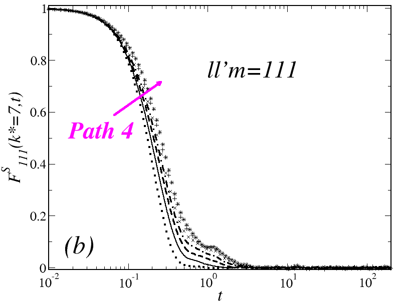
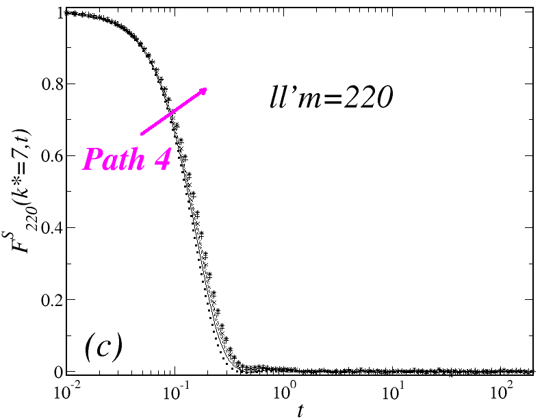
Figure 4: (Color online) Time evolution of the correlation functions (a) $F_{110}(k^{*},t)$, (b) $F_{111}(k^{*},t)$ and (c) $F_{220}(k^{*},t)$ evaluated at $k^{*}=5.3$, along the isotherm $T^{*}=1$, for different concentrations (as indicated).

The angular MSD, $W_{\theta}(t)$, describes consistently the same scenario for the arrest of the orientational dynamics. Along Paths 1 and $2$ (Fig. 5(a) and Fig. 5(b), respectively) $W_{\theta}(t)$ reaches its ergodic saturation value within the range $0.1\leq T^{*}\leq 2$. As it may be expected, the time elapsed to reach this limit becomes progressively larger with decreasing temperature. Below this range, $W_{\theta}(t)$ saturates to a smaller value, thus indicating arrest in the diffusion of the ODF. For the isochore $\eta=0.6$, the angular MSD rapidly reaches the ergodic value for temperatures down to $T^{*}=0.5$. At $T^{*}=0.2$, however, this requires the whole time-window of the simulations. For even lower temperatures, within the same time window, $W_{\theta}(t)$ appears fully arrested. Finally, this observable remains unaffected at the isochore $T^{*}=1.0$ (Fig. 5(d))

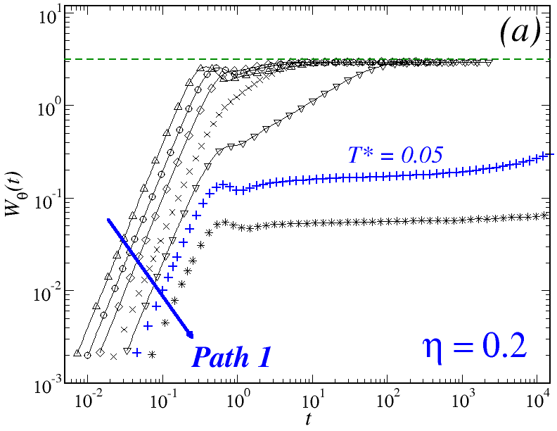
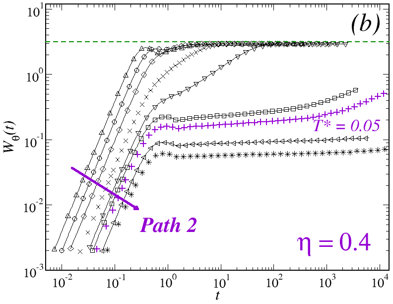
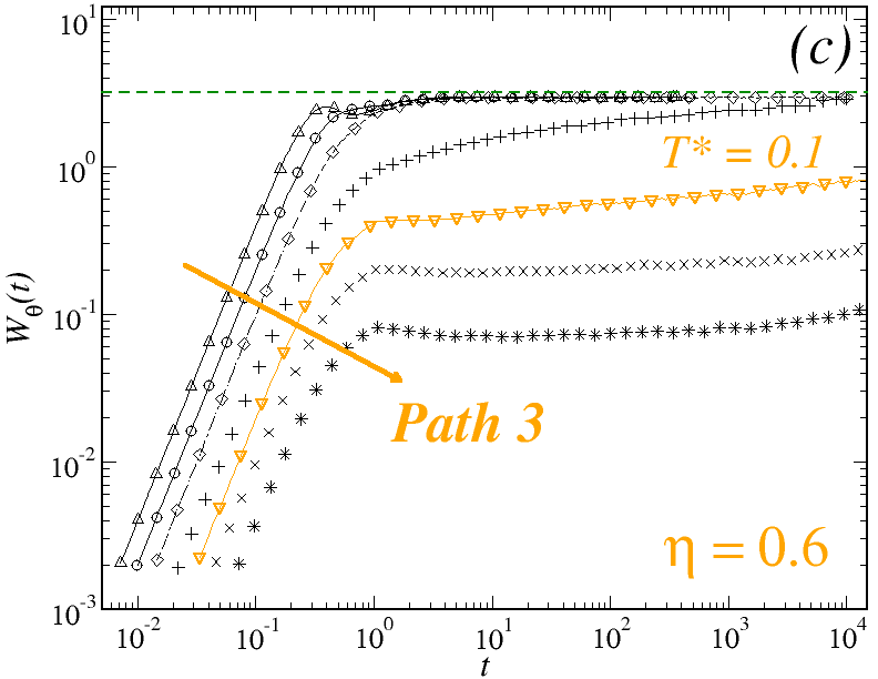
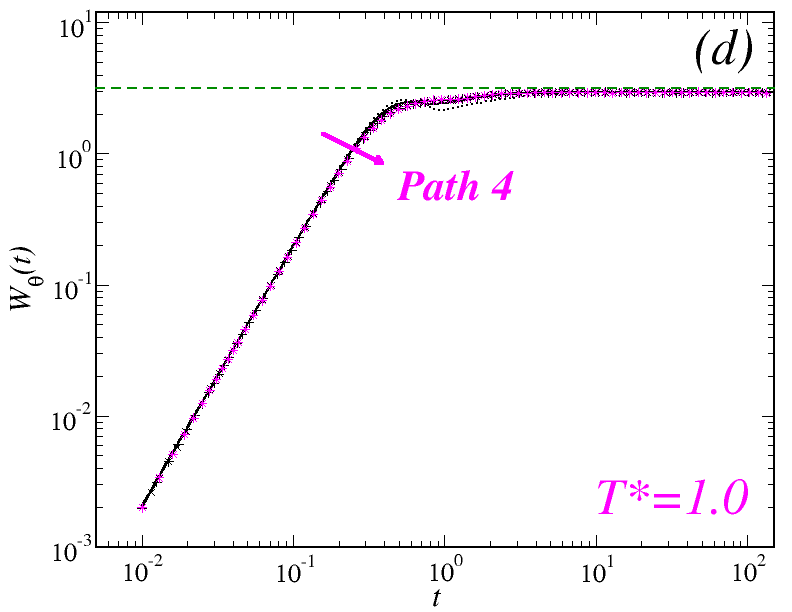
Figure 5: (Color online) Behavior of the angular mean square displacement, $W_{\theta}(t)$, at the three isochores (a) $\eta=0.2$, (b) $\eta=0.4$ and (c) $\eta=0.6$, for different temperatures; and for the isotherm (d) $T^{*}=1.0.$ Symbols are used exactly as in Figs. 3 and 5 above to represent the state points. The (green) dashed horizontal lines indicate the ergodic long time value of $W_{\theta}$ and are used as guide to the eye.

To summarize, the MD simulations exhibit three different scenarios for dynamical arrest in the model. The first occurs at low and intermediate concentrations upon lowering the temperature and is mainly characterized by the simultaneous arrest of the TDF and ODF, with both dynamics being strongly coupled. Neither the critical temperature of this transition, nor the corresponding localization length of the constitutive particles, vary significantly with $\eta$, despite qualitative changes observed in the structural behavior of the system upon increasing the density. A second scenario is observed at high densities and high-to-intermediate temperatures, where only the dynamics of the TDF undergoes arrest whilst the ODF remain ergodic. This indicates the possibility of partially arrested states to occur, either through an isochorical drop in temperature, or an isothermal compression. This transition presents the features of the GT in dense HS fluids. Finally, a third possibility involves the arrest of the orientational dynamics by cooling down the system from a partially arrested state. This was observed to occur at temperatures only slightly higher with respect to those describing simultaneous arrest.

IV Theoretical development

To provide a more comprehensive picture of the dynamical arrest transitions of a dipolar fluid, we now consider the SCGLE theory. Specifically, we use this theoretical framework to obtain the GT lines in the full parameter space of the system, leading to the development of an arrested states diagram which identifies the regions in the $(\eta,T^{*})$-plane where the system remains ergodic, the regions where it becomes partially or fully arrested, and the boundaries between such regions. This kinetic arrest diagram complements the usual equilibrium phase diagram goyal1 ; goyal2 ; goyal3 . As we show below, the physical scenario outlined by the SCGLE describes consistently the dynamical features of the simulations and organizes qualitatively the different state points and Paths studied with MD, thus providing mutual support between the results of the two independent approaches.

The use of the SCGLE for this purpose is particularly helpful because the precise determination of GT points from simulations is notoriously difficult. Close to a transition, one typically encounters strong instabilities and very slow dynamics with history dependence, which renders the required computational time excessively large. Furthermore, the common protocols to estimate GT points in simulations are normally based on extrapolations of either the divergence of the relaxation time of the ISFs or the diffusion coefficients, and are therefore prone to errors, since this intrinsically involves a large uncertainty in the choice of the specific extrapolation function and the fit range.

IV.1 Arrested states diagram

We briefly recall some technical aspects regarding the determination of GT lines within SCGLE (for more details the reader is referred to appendix C below, and to Ref. Elizondo-PRE-2014 ). The theory provides a self-consistent system of equations describing the full wave-vector and time dependence of the diagonal ($l=l^{\prime}$) ISFs, $F_{ll^{\prime}m}(k,t)\delta_{ll^{\prime}}\equiv F_{lm}(k,t)$, and their corresponding self counterparts $F^{S}_{ll^{\prime}m}(k,t)\delta_{ll^{\prime}}\equiv F^{S}_{lm}(k,t)$. Close to conditions of dynamical arrest, one can develop a generic asymptotic solution for these equations, leading to a new closed set of equations for the non-decaying $k$-components of both $F_{lm}(k,t)$ and $F^{S}_{lm}(k,t)$, commonly referred to as non-ergodicity parameters (NEP), and defined as $\displaystyle{\lim_{t\to\infty}F_{lm}(k,t)}/F_{lm}(k,t=0)\equiv f_{lm}(k)$ and $\displaystyle{\lim_{t\to\infty}F^{S}_{lm}(k,t)}\equiv f^{S}_{lm}(k)$.

Upon a well defined set of approximations, the equations for $f_{lm}(k)$ and $f^{S}_{lm}(k)$ can be rewritten as only two equations for the parameters $\gamma_{T}$ and $\gamma_{R}$, which play the role of order parameters in the determination of the ergodic-to-non-ergodic transitions of the dynamics of, respectively, the TDF and ODF (Eqs. (29) and (30) of appendix C) . In terms of these quantities, fully ergodic (fluid) states are described by the condition that both, $\gamma_{T}^{-1}$ and $\gamma_{R}^{-1}$, are equal to zero. Any other solution indicates loss of ergodicty (i.e., dynamical arrest) in one or both degrees of freedom. For instance, the condition $\gamma_{T}^{-1}\neq 0$ and $\gamma_{R}^{-1}=0$ describes partially arrested states, where only the TDF undergo a GT, whereas the dynamics of the ODF remains ergodic. Similarly, the condition $\gamma_{T}^{-1}\neq 0$ and $\gamma_{R}^{-1}\neq 0$ describes arrest in both degrees of freedom, i.e., fully arrested states.

To solve the equations for $\gamma_{T}$ and $\gamma_{R}$, one requires the previous determination of the diagonal elements, $S_{lm}(k)$, of the spherical harmonics expansion of the static structure factor (SSF) $S(k,\bm{\mu},\bm{\mu}^{\prime})$, at each state point of the parameters space (notice that $S_{ll^{\prime}m}(k)=F_{ll^{\prime}m}(k,t=0)$ and $S_{ll^{\prime}m}(k)\delta_{ll^{\prime}}\equiv S_{lm}(k)$). In general, this might pose a non-trivial problem on its own right. To simplify the theoretical calculations as much as possible, we have approximated the $S_{lm}(k)$ components of the simulated model system by a softened-core version of Wertheim’s solution for the mean spherical model (MSM) of a dipolar hard-sphere fluid (DHS) wertheim . The specific details of this approximation are provided in appendix D.

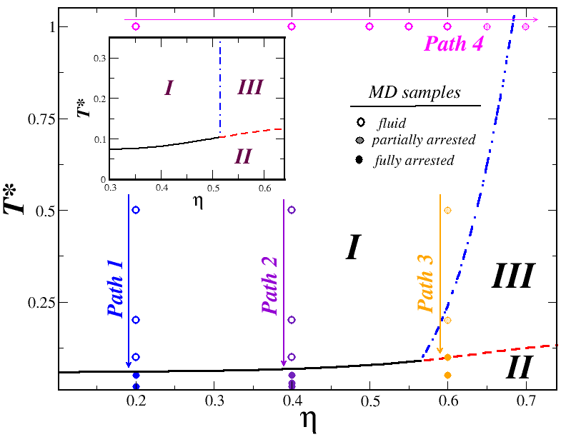
Figure 6: State space of the dipolar fluid. The different symbols and arrows denote, respectively, the state points and Paths studied via MD simulations. Open circles are used to represent the ergodic samples, half-filled circles describe samples where partially arrested states are observed, solid circles account for full arrest. The lines delimiting regions I, II and III are predictions of the SCGLE for three distinct GT lines using the approximation described in appendix D for the static structure factor projections, $S_{lm}(k)$. Inset: analogous results of the SCGLE for a DHS system previously reported in Ref. Elizondo-PRE-2014 .

Hence, one uses $S_{lm}(k)$ to solve the equations for $\gamma_{T}$ and $\gamma_{R}$ at every state point of the ($\eta,T^{*}$) plane. This leads to the identification of three kinetically different regions separated by three distinct transition lines. Our results are summarized in Fig. 6, where we also show the location of the state points and Paths investigated via MD. Based on the theory, the $(\eta,T^{*})$ space can be partitioned as follows: a fluid region (I) where the dynamics of both TDF and ODF remain ergodic ($\gamma_{T}^{-1}=\gamma_{R}^{-1}=0$). This region is delimited by two different boundaries. One of these boundaries (black solid line) describes the transitions to fully arrested states (II), where $\gamma_{T}$ and $\gamma_{R}$ become finite simultaneously, so both degrees of freedom are dynamically arrested. The second boundary (blue dashed-pointed line), instead, describes the transitions to partially arrested states (III) where only the TDF dynamics undergo arrest ($\gamma_{T}$-finite) whereas the ODF remain ergodic ($\gamma_{R}^{-1}=0$). Finally, a third line (red dashed) separates regions II and III, thus describing the arrest of the ODF under the condition that the TDF were previously arrested.

The I$\to$II transition line represents the behavior of the critical temperature, $T^{*(g)}_{I\to II}(\eta)$, as a function of the volume fraction as predicted by the SCGLE. It describes a monotonically (and very slowly) increasing function of $\eta$ and, noticeably, $T^{*(g)}_{I\to II}(\eta=0.2)\approx T^{*(g)}_{I\to II}(\eta=0.4)\approx 0.06$, which is in remarkable agreement with our previous findings with MD along Paths $1$ and $2$.

The theory predicts that this line bifurcates into two distinct lines upon increasing the concentration ($\eta\approx 0.57$). The branch describing the I$\to$III transition shows that the critical temperature $T^{*(g)}_{I\to III}(\eta)$ increases significantly with small increments in $\eta$. This implies strong effects of crowding in the slowing down of the translational dynamics and a remarkable decoupling between translational and orientational dynamics as this transition is approached. This feature is also qualitatively consistent with the scenario outlined by the simulations along Paths $3$ and $4$, although some small quantitative differences are observed. For example, the theory seems to slightly overestimate the critical volume fraction of the bifurcation point and of the I$\to$III transition. This may be attributed to deviations of the simplified model assumed in the theory from the simulated system, and also to the approximations carried out to determine the structure factor projections, $S_{lm}(k)$ (appendix D). Nevertheless, the overall physical scenario is essentially the same.

Starting from a state point inside the partially arrested region III and decreasing the temperature one crosses the II$\to$III transition line, below which, the orientational dynamics of the positionally-frozen dipoles also becomes arrested. Hence, this line describes a scenario similar to a spin glass-like transition. Notice that the critical temperature $T^{*(g)}_{II\to III}(\eta)$ appears almost independent on $\eta$ and satisfies $T^{*(g)}_{II\to III}\approx 0.1$, a value in good quantitative agreement with the simulation results for Path 3.

One can also also compare these results against the predictions of the SCGLE corresponding to a DHS model Elizondo-PRE-2014 , i.e., a system where the short-ranged and purely repulsive contribution to the potential is represented by the discontinuous (athermal) HS potential, and not by the soft (thermal) WCA interaction considered in both theory and simulations for this work. This is shown in the inset of Fig. 6. Clearly, the main difference between the two diagrams only refers to the slope of the I-III transition line. In the case of the DHS model, this is described by a vertical line at $\eta^{(g)}_{DHS}\approx 0.52$, which results from the athermal nature of the discontinuous HS potential and, consequently, of the I-III transition in the case of the DHS model. Crucially, however, the topology of the two diagrams is identical despite the rather different range of the anisotropic dipolar forces and torques in each case: the DHS model uses a genuine dipole-dipole potential, which considers a $r^{-3}$ contribution in all the space. In the simulated system, in contrast, we have truncated this interaction for simplicity. This indicates that the topology of the dynamical arrest scenario of a dipolar fluid is essentially determined by the anisotropy of the dipolar tensor $D(\mathbf{r}_{ab},\bm{\hat{\mu}}_{a},\bm{\hat{\mu}}_{b})\equiv\bm{\hat{\mu}}_{a}\cdot\bm{\hat{\mu}}_{b}-3(\bm{\hat{\mu}}_{a}\cdot\hat{\mathbf{r}}_{ab})(\bm{\hat{\mu}}_{b}\cdot\hat{\mathbf{r}}_{ab})$ (see Eq. (3) above), and not by the specific range of the pair potential. This provides support to the systematic use of truncated anisotropic potentials for the study of glassy behavior in dipolar systems which, as mentioned above, simplifies considerably the simulations, since one avoids the specialized treatment of long-ranged forces and torques.

V Conclusions

Molecular dynamics simulations and theoretical calculations were combined to investigate the glassy behavior and different non-equilibrium phases and transitions in a dipolar fluid. The system was modeled as a collection of $N$ spherical particles interacting via a soft-repulsive potential coated with an anisotropic contribution that retains the directional features of the dipole-dipole forces, but which neglects its long-ranged character. This is a reasonable approximation for dipolar colloids suspended in highly dielectric solvents. An advantage of this modeling procedure is that the simulations are not too computationally exhaustive.

We have studied the dynamics associated to the translational and orientational degrees of freedom, at different regions of the parameter space of the system, and considering distinct pathways to dynamical arrest. The detailed analysis of several correlation functions and of two types of mean square deviations along the distinct Paths, provided evidence of the occurrence of three types of dynamical arrest transitions in a dipolar fluid.

At small and intermediate volume fractions, one observes the simultaneous arrest of the dynamics of both degrees of freedom on cooling, occurring at a critical temperature $T_{\emph{I}\to\emph{II}}^{(g)}\approx 0.05$. Despite some qualitative changes observed in the structure of the simulated system, this transition seems to not depend crucially on the concentration. Both simulations and theory support this interpretation. At high concentration, instead, a bifurcation scenario for the glass transition is found. In this regime, a decoupling in the dynamics of each degree of freedom leads to another type of transition describing partially arrested states, where only the translational motion becomes arrested, but with the orientations remaining ergodic. In this regard, it is also important to notice that neither in the simulations nor in the theory we observed any hint of the other possible mixed state, in which the translational motion remains ergodic, but with the orientations become arrested. Finally, a third kind of transition can be reached starting from a partially arrested state and decreasing the temperature, with the orientational correlations displaying arrest under the condition that the translational dynamics was already arrested.

The physical scenario outlined by the simulations is qualitatively (and semi quantitatively) consistent with the results of the SCGLE theory. The latter, however, allows us to develop a more generic description of dynamical arrest in the dipolar fluid. This was conveniently summarized in an arrested states diagram, which results topologically identical to that of a dipolar hard sphere fluid, where different short and long-range interactions are considered. This indicates that our results may be generic to systems with competing dynamics arising from dipolar anisotropic forces and torques. These observations could also be relevant for the understanding of glassy dynamics in a wider range of colloidal systems dealing with higher order multipolar contributions (for instance, quadrupolar moments) or more complicated interactions (Janus particles).

Let us also mention that the present work is also an essential and unavoidable first step in a more ambitious program towards a deeper study of the non-equilibrium and nonstationary phenomena, such as the kinetics of the aging associated with these transitions. As it happens, the SCGLE formalism has recently been extended to describe non-stationary non-equilibrium structural relaxation processes, such as aging or the dependence of the dynamical and structural properties on the protocol of fabrication, in liquids constituted by particles interacting through non spherical potentials nescgle7 . The resulting non-equilibrium self-consistent generalized Langevin equation theory, aimed at describing non-equilibrium phenomena in general, leads in particular to a simple and intuitive (but still generic) description of the essential behavior of glass-forming dipolar liquids near and beyond its dynamical arrest transitions. This renders the description of the nonequilibrium processes occurring in a colloidal dispersion after an instantaneous temperature quench possible, with the most interesting prediction being the aging processes occurring when full equilibration is prevented by conditions of dynamical arrest. In this regard, the development of the arrest diagram presented in this contribution, and its validation by independent results obtained with the assistance molecular dynamics simulations constitutes a crucial step in developing a full description of dynamical arrest in dipolar liquids.

Finally, we expect that the results of this work might serve to locate and reinterpret previous results dealing with both equilibrium and arrested dynamics in dipolar fluids, and as a benchmark for future tests in similar models with competitive dynamics arising from distinct degrees of freedom. The information provided in this work might be also relevant for the rational design of technologically important materials based in ferrofluids, considering dipolar systems as prototypical models. Our work is part of a long term investigation meant to provide insight in the non-equilibrium behavior of various anisotropic systems, such as suspensions of particles with higher order multipolar moments, and more complicated interactions, for instance, Janus suspensions. Both characterizations will be reported in further communications elsewhere.

Appendix A Mean square deviations and rotational diffusion coefficients

To extract rotational diffusion coefficients from saturating MSDs one can start with the solution of Fick’s equation for the orientational microscopic density, $\rho(\theta,\phi,t)$, on a spherical surface

$$\frac{\partial}{\partial t}\rho(\theta,\phi,t)=D_{R}\nabla_{s}^{2}\rho(\theta,\phi,t),$$ (12)

where $\nabla_{s}^{2}$ is the Laplace-Beltrami operator acting over the surface of the sphere. For an initial condition given by a delta function on $\theta=0$ (the north pole), the solution found by Perrin perrin-1928 reads

$$\rho(\theta,t)=\sum_{l=0}^{\infty}\frac{2l+1}{4\pi}P_{l}(\cos\theta)e^{-l(l+1)D_{R}t},$$ (13)

with $P_{l}(\cos\theta)$ being Legendre polynomials. Using this solution, one can calculate the mean square deviation in the polar angle, $W_{\theta}(t)\equiv\langle\theta^{2}(t)\rangle$, via integration

$$W_{\theta}(t) = \sum_{l=0}^{\infty}\frac{2l+1}{2}\,e^{-l(l+1)D_{R}t}\int_{0}^{\pi}\theta^{2}P_{l}(\cos\theta)\sin\theta\,d\theta$$

$$= a_{0}+a_{1}e^{-2D_{R}t}+a_{2}e^{-6D_{R}t}+a_{3}e^{-12D_{R}t}+...$$

where the coefficients $a_{i}$ ($i=0,1,2,...$) are easily calculated, and with the first two being $a_{0}=(\pi^{2}-4)/2$ and $a_{1}=-3\pi^{2}/8$. Using this result, one may write

$$\log(a_{0}-W_{\theta}(t))=\log|a_{1}|-2D_{R}t+\log\left(1+b_{2}e^{-4D_{R}t}+...\right).$$ (15)

with $b_{i}$, $i=2,3...$ being simple geometrical constants given in terms of $a_{i}$. Since terms of the form $e^{-nD_{R}t}$ decay very fast with increasing $n$, one can make the approximation

$$\log(a_{0}-W_{\theta}(t))\approx\text{const.}-2D_{R}t.$$ (16)

Using the orthogonality of the Legendre polynomials, Perrin also found a closed form for $W_{\sin\theta}(t)\equiv\langle\sin^{2}\theta(t)\rangle$, which reads

$$W_{\sin\theta}(t)=\frac{2}{3}\left(1-e^{-6D_{R}t}\right).$$ (17)

These two forms can be used, in principle, to get a well-defined value for the rotational diffusion coefficient. In particular, using the previous equation, one can write

$$\log\left(1-\frac{3}{2}W_{\sin\theta}(t)\right)=-6D_{R}t.$$ (18)

One should take into account, however, that for numerical work the usefulness of eqs. (16) and (18) is severely limited by the fact that, as $t$ grows, the argument of the log function gets very close to zero and the noise overwhelms the signal. Yet, with good statistics, one may get a fair estimation of the value of $D_{R}$.

Appendix B Radial distribution function

Besides the analysis of the dynamics, we have monitored the structural behavior of the simulated fluid, represented by the radial distribution function $g(r)$, and along the four Paths considered. The results are shown in Fig. 7 (data are shifted in the vertical axis for clarity).

At the isochore $\eta=0.2$ (Path 1, Fig. 7(a)) and high temperatures, $g(r)$ exhibits a single broad peak centered at $r\approx 1.2\sigma_{ave}$, beyond which $g(r)$ attains its asymptotic unit value. Upon cooling, this first diffuse peak evolves and reveals that is in reality the superposition of the nearest-neighbor peaks of $g_{11}(r)$, $g_{12}(r)$, and $g_{22}(r)$, separated from each other by approximately $\pm\sigma_{ave}/6$. At $T^{*}=0.05$ and below, the amplitude of the three peaks become noticeable higher. At the same time, one observes the emergence of an additional train of smaller peaks, now centered at $r\approx 2\sigma_{ave}$ representing the second-nearest neighbor shell. The various individual peaks in this train correspond to the combinations of small and large particles in an approximately linear configuration. This may reflect the tendency of the dipolar particles to associate in linear trimers and small chains.

By increasing the volume fraction to $\eta=0.4$, the structure evolves to that of a liquid (Path 2, Fig. 7(b)), characterized by the emergence of a main peak and followed by other well-separated, but smaller, secondary peaks. Importantly, the small oscillations around $r\approx 2\sigma_{ave}$ observed in $g(r)$ along Path 1 and at low temperatures disappear. For clarity in the comparison, we do not show the behavior of $g(r)$ at the state points ($\eta=0.4,T^{*}=0.07$) and ($0.4,T^{*}=0.03$).

At both the isochore $\eta=0.6$ (Path 3, Fig. 7(c)) and the isotherm $T^{*}=1$ (Path 4, Fig. 7(d)), $g(r)$ presents the typical evolution in a dense liquid with short ranged repulsion.

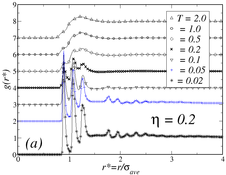
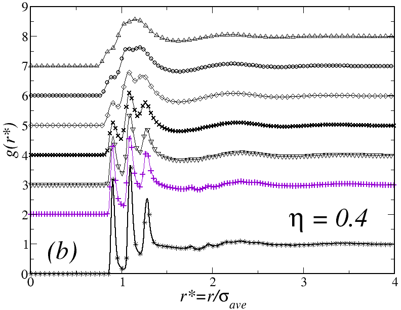
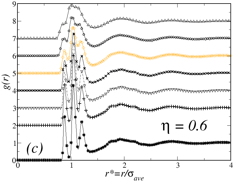
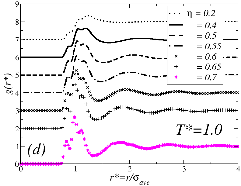
Figure 7: (Color online) Evolution of the radial distribution function, $g(r)$ along the three ischores (a) $\eta=0.2$ (Path 1), (b) $\eta=0.4$ (Path 2), (c) $\eta=0.6$ (Path 3), and along the isotherm, $T^{*}=1$ (Path 4).

Appendix C SCGLE theory for Brownian fluids of non-spherical particles

The SCGLE theory of colloid dynamics and dynamical arrest has been previously extended for the description of Brownian fluids constituted by particles interacting through non-spherical potentials. For more details the reader is referred to Elizondo-PRE-2014 . In its simplest version, the SCGLE formalism provides a closed set of time evolution equations for the diagonal components ($l=l^{\prime}$, $m=m^{\prime}$) $F_{lm}(k,t)$ and $F^{S}_{lm}$, of the ISFs defined in Eqs. (10) and (11). Written in the Laplace space, such equations read

$$F_{lm}(k,z)=\frac{S_{lm}(k)}{z+\displaystyle\frac{k^{2}D_{T}^{0}S^{-1}_{lm}(k)}{1+\Delta\zeta_{T}^{*}(z)\lambda^{(lm)}_{T}(k)}+\frac{l(l+1)D_{R}^{0}S^{-1}_{lm}(k)}{1+\Delta\zeta_{R}^{*}(z)\lambda^{(lm)}_{R}(k)}}$$ (19)

and

$$F_{lm}^{S}(k,z)=\frac{1}{z+\displaystyle\frac{k^{2}D_{T}^{0}}{1+\Delta\zeta_{T}^{*}(z)\lambda^{(lm)}_{T}(k)}+\frac{l(l+1)D_{R}^{0}}{1+\Delta\zeta_{R}^{*}(z)\lambda^{(lm)}_{R}(k)}}.$$ (20)

where, $D_{R}^{0}$ is the rotational free-diffusion coefficient, and $D^{0}_{T}$ is the center-of-mass translational free-diffusion coefficient, whereas the functions $\lambda^{(lm)}_{T}(k)$ and $\lambda^{(lm)}_{R}(k)$ are defined as $\lambda^{(lm)}_{T}(k)=1/[1+(k/k_{c})^{2}]$ and, for simplicity, $\lambda^{(lm)}_{R}(k)=1$, where $k_{c}=\alpha\times k_{max}$, with $k_{max}$ being the position of the main peak of $S_{00}(k)$ and $\alpha=1.305$. This ensures that, for radially-symmetric interactions, one recovers the original theory describing liquids of soft and hard spheres.

On the other hand, within a well defined set of approximations (discussed in appendix A of Ref. Elizondo-PRE-2014 ) the functions $\Delta\zeta_{\alpha}^{*}(t)$ ($\alpha=T,R$) may be written as

$$\Delta\zeta^{*}_{T}(t)=\frac{1}{3}\frac{D_{T}^{0}}{(2\pi)^{3}n}\int d\mathbf{k}k^{2}\sum_{l}\left[{2l+1}\right]\left[1-S^{-1}_{l0}(k)\right]^{2}F^{S}_{l0}(k;t)F_{l0}(k;t)$$ (21)

and

$$\Delta\zeta^{*}_{R}(t)=\frac{1}{2}\frac{D_{R}^{0}}{(2\pi)^{3}}\frac{n}{4}\frac{1}{(4\pi)^{2}}\int d\mathbf{k}\sum_{l,m}\left[2l+1\right]h^{2}_{l0}(k)\left[A_{l;0m}\right]^{2}\left[S^{-1}_{lm}(k)\right]^{2}F^{S}_{lm}(k;t)F_{lm}(k;t)$$ (22)

where $h_{lm}(k)$ denotes the diagonal k-frame projections of the total correlation function $h(\mathbf{k},\bm{\Omega},\bm{\Omega}^{\prime})$, i.e., $h_{lm}(k)$ is related to $S_{lm}(k)$ by $S_{lm}(k)=1+(n/4\pi)h_{lm}(k)$, and $n=N/V$ is the number density. Finally, $A_{l;mm^{\prime}}\equiv\left[C_{lm}^{+}\delta_{m+1,m^{\prime}}+C_{lm}^{-}\delta_{m-1,m^{\prime}}\right]$ and $C_{lm}^{\pm}\equiv\sqrt{(l\mp m)(l\pm m+1)}$.

The closed set of coupled equations (19)-(22) constitute the equilibrium non spherical version of the SCGLE theory, whose solution provides the full wave vector and time dependence of the dynamic correlation functions $F_{lm}(k;t)$ and $F^{S}_{lm}(k;t)$ and of the memory functions $\Delta\zeta^{*}_{\alpha}(t)$. These equations may be numerically solved using standard methods once the projections $S_{lm}(k)$ of the static structure factor are provided. Under some circumstances, however, one may only be interested in identifying and locating the regions in state space of a given system that correspond to the various possible ergodic or non ergodic phases, involving the dynamical arrest of the dynamics of the translational and orientational degrees of freedom. For this purpose it is possible to derive from the full SCGLE equations the so-called bifurcation equations, i.e., the equations for the long-time stationary solutions of equations (19)-(22). These are written in terms of the so-called non-ergodicity parameters, defined as

$$f_{lm}(k)\equiv\lim_{t\to\infty}\frac{F_{lm}(k;t)}{S_{lm}(k)},$$ (23)

$$f^{S}_{lm}(k)\equiv\lim_{t\to\infty}F^{S}_{lm}(k;t),$$ (24)

and

$$\Delta\zeta_{\alpha}^{*(\infty)}\equiv\lim_{\tau\to\infty}\Delta\zeta_{\alpha}^{*}(t),$$ (25)

with $\alpha=T,R$. The simplest manner to determine these asymptotic solutions is to take the long-time limit of Eqs. (19)-(22), leading to a system of coupled equations for $f_{lm}(k)$, $f^{S}_{lm}(k)$, and $\Delta\zeta_{\alpha}^{*(\infty)}$.

It is not difficult to show that the resulting equations can be written as

$$f_{lm}(k)=\frac{\left[S_{lm}(k)\right]\lambda_{T}^{(lm)}(k)\lambda_{R}^{(lm)}(k)}{S_{lm}(k)\lambda_{T}^{(lm)}(k)\lambda_{R}^{(lm)}(k)+k^{2}\gamma_{T}\lambda_{R}^{(lm)}(k)+l(l+1)\gamma_{R}\lambda_{T}^{(lm)}(k)}$$ (26)

and

$$f^{S}_{lm}(k)=\frac{\lambda_{T}^{(lm)}(k)\lambda_{R}^{(lm)}(k)}{\lambda_{T}^{(lm)}(k)\lambda_{R}^{(lm)}(k)+k^{2}\gamma_{T}\lambda_{R}^{(lm)}(k)+l(l+1)\gamma_{R}\lambda_{T}^{(lm)}(k)},$$ (27)

where the dynamic order parameters $\gamma_{T}$ and $\gamma_{R}$, defined as

$$\gamma_{\alpha}\equiv\frac{D^{0}_{\alpha}}{\Delta\zeta_{\alpha}^{*(\infty)}},$$ (28)

are determined from the solution of

$$\frac{1}{\gamma_{T}}=\frac{1}{6\pi^{2}n}\displaystyle{\int_{0}^{\infty}}dk\,k^{4}\sum_{l}[2l+1]\left[1-S^{-1}_{l0}(k)\right]^{2}S_{l0}(k)f^{S}_{l0}(k)f_{l0}(k),$$ (29)

and

$$\frac{1}{\gamma_{R}}=\frac{1}{16\pi^{2}n}\displaystyle{\int_{0}^{\infty}}dkk^{2}\sum_{lm}[2l+1][S_{l0}(k)-1]^{2}S^{-1}_{lm}(k)f^{S}_{lm}(k)f_{lm}(k)A_{l;0m}^{2}.$$ (30)

Fully ergodic states are thus described by the condition that the non-ergodicity parameters (i.e., $f_{lm}(k)$, $f^{S}_{lm}(k)$, and $\Delta\zeta_{\alpha}^{*(\infty)}$) are all zero, so the dynamic order parameters $\gamma_{T}$ and $\gamma_{R}$ are both infinite. Any other possible solution of these bifurcation equations indicate total or partial loss of ergodicity. Thus, $\gamma_{T}$ and $\gamma_{R}$ finite indicate full dynamic arrest whereas $\gamma_{T}$ finite and $\gamma_{R}=\infty$ corresponds to the mixed state in which the translational degrees of freedom are dynamically arrested but not the orientational degrees of freedom.

Appendix D Determination of the static structure factor projections, $S_{lm}(k)$, for a dipolar soft sphere fuid.

As mentioned above, the solution of Eqs. (19)-(22) and (29)-(30) requires the previous determination of the spherical harmonics projections $S_{lm}(k)$, of the static structure factor of the system under consideration, or equivalently, the projections, $c_{lm}(k)$, of the direct correlation function. Both quantities are related through the Ornstein-Zernike (OZ) equation $S_{lm}(k)=\left[1-\displaystyle{\frac{n}{4\pi}c_{lm}(k)}\right]^{-1}$.

For this, one starts by identifying the system of interest, which thus require the specific form of the two-particle potential of interaction, $U^{ab}(\mathbf{r}_{ab},\hat{\bm{\mu}}_{a},\hat{\bm{\mu}}_{b})$. To represent the simulated system, such pairwise potential should possess the generic form

$$U^{ab}(\mathbf{r}_{ab},\hat{\bm{\mu}}_{a},\hat{\bm{\mu}}_{b})=U_{REP}^{ab}(\mathbf{r}_{ab})+U^{ab}_{DIP}(\mathbf{r}_{ab},\hat{\bm{\mu}}_{a},\hat{\bm{\mu}}_{b})$$ (31)

,

with $U_{REP}^{ab}(\mathbf{r}_{ab})$ describing a short-ranged repulsive potential and $U^{ab}_{DIP}(\mathbf{r}_{ab},\hat{\bm{\mu}}_{a},\hat{\bm{\mu}}_{b})$ an anisotropic dipolar contribution. This generic representation includes as a particular case the dipolar hard-sphere model (DHS), where $U_{REP}^{ab}$ is given by the discontinuous hard-sphere potential and $U^{ab}_{DIP}$ by the dipole-dipole potential, but it also includes other possible systems. For instance, under some circumstances it may be necessary to consider some degree of softness in the purely repulsive part, just as it happens in the case of the Stockmayer potential stockmayer , which replaces $U_{REP}^{ab}$ by a Lennard-Jones potential. In general, any such departure from the DHS reference potential will destroy the analytical convenience provided by the solution of Wertheim for the Mean Spherical Model (MSM) wertheim which renders the calculation of the functions $c_{lm}(k)$ straightforward.

A simplified version of the Stockmayer potential which allows to exploit the analytical simplicity of Wertheim’s solution, consist in replacing $U_{REP}^{ab}$ by the WCA potential of Eq. (2). In this manner, the generic potential of Eq. (31) can be written as the following soft-sphere dipolar potential

$$U^{ab}_{SSD}(\mathbf{r}_{ab},\hat{\bm{\mu}}_{a},\hat{\bm{\mu}}_{b})=U_{WCA}^{ab}(\mathbf{r}_{ab})+\frac{\epsilon^{ab}_{\text{\tiny{DIP}}}}{(r_{ab}/\sigma)^{3}}[\bm{\hat{\mu}}_{a}\cdot\bm{\hat{\mu}}_{b}-3(\bm{\hat{\mu}}_{a}\cdot\hat{\mathbf{r}}_{ab})(\bm{\hat{\mu}}_{b}\cdot\hat{\mathbf{r}}_{ab})]$$ (32)

,

where, in the case of a monodisperse system, $\epsilon^{ab}_{\small{DIP}}=\mu^{2}/\sigma^{3}$ is the energy scale of the dipolar contribution. A further simplification arises when one considers $\epsilon^{ab}_{WCA}=\epsilon^{ab}_{DIP}$

In the spirit of the WCA treatment of soft-core interactions hansen , we may assume that the properties of the soft-core dipolar potential of Eq. 32 can be approximated by those of an effective DHS potential $U^{eff}_{DHS}(\mathbf{r}_{ab},\hat{\bm{\mu}}_{a},\hat{\bm{\mu}}_{b})$ with a state-dependent effective diameter $\sigma^{eff}(n,T)$, i.e., by a system with a potential of interaction

$$U^{eff}_{DHS}(\mathbf{r}_{ab},\hat{\bm{\mu}}_{a},\hat{\bm{\mu}}_{b})=U^{eff}_{HS}(r;\sigma^{eff})+\frac{\epsilon^{ab(eff)}_{DIP}}{(r/\sigma^{eff})^{3}}[\bm{\hat{\mu}}_{a}\cdot\bm{\hat{\mu}}_{b}-3(\bm{\hat{\mu}}_{a}\cdot\hat{\mathbf{r}}_{ab})(\bm{\hat{\mu}}_{b}\cdot\hat{\mathbf{r}}_{ab})]$$ (33)

where $\epsilon^{ab(eff)}_{DIP}$ is defined as $\epsilon^{ab(eff)}_{DIP}\equiv\lambda{-3}\epsilon^{ab}_{DIP}$, and with $\lambda\equiv\sigma^{eff}(n,T)/\sigma$. The similarity between the WCA and the HS potentials leads to the additional simplification that $\sigma_{HS}(n,T)$ becomes $n$-independent, and given by the ”blip function” approximation hansen .

Therefore, within these assumptions, the direct correlation function $c_{SSD}((\mathbf{r}_{ab},\hat{\bm{\mu}}_{a},\hat{\bm{\mu}}_{b});n,T)$ of a soft dipolar system with a potential defined by Eq. 32 can be approximated by the direct correlation function of an effective DHS system, $c^{eff}_{DHS}(\mathbf{r}_{ab},\hat{\bm{\mu}}_{a},\hat{\bm{\mu}}_{b};n,T)$. In dimensionless units, this approximation reads

$$c_{SSD}(\mathbf{r}/\sigma,\hat{\bm{\mu}}_{1},\hat{\bm{\mu}}_{2};n^{*},T^{*})\approx c_{DHS}(\mathbf{r}/\lambda\sigma,\hat{\bm{\mu}}_{1},\hat{\bm{\mu}}_{2};\lambda^{3}n^{*},\lambda^{-3}T^{*}).$$ (34)

Clearly, introducing again the MSA for the calculation of the right side of this equation restores the analytical simplicity of Wertheim’s solution by means of a simple re-scaling procedure. From here, the determination of the projections $c_{lm}(k)$ is straightforward (see, for instance, appendix E of Ref. schilling-PRE-1997 )

References

- (1) S.C. Glotzer and M.J. Solomon, Nat. Mater., 2007 6(8), 557-562, doi:10.1038/nmat1949.
- (2) O. Cayre, V.N. Paunov and O.D. Velev, Chem. Commun., 2003, (18), 2296-2297.
- (3) A. Walther ad A.H.E. Müller Chem. Rev., 2013, 113(7), pp 5194-5261.
- (4) J. Zhang†, B.A. Grzybowski and S. Granick, Langmuir, 2017, 33(28), 6964-6977.
- (5) S.A. Safran, Nature Materials 2, 71-72. (2003).
- (6) Nych A. et.al. Assembly and Control of 3D Nematic Dipolar Colloidal Crystals, Nat. Commun. 4:1489 doi: 10.1038/ ncomms2486 (2013).
- (7) K. Butter, P.H.H. Bomans, P.M. Frederik, G.J. Vroege and A.P. Philipse, Nature Materials 2, 88-91 (2003).
- (8) A. Yethiraj and A. van Blaaderen, Nature 421 513-517 (2003). DOI:10.1038/nature01328.
- (9) T. Tlusty and S.A. Safran, Science 290, 1328 (2000).
- (10) K. Klokkenburg, B.H. Erné, A. Wiedenmann, A.V. Petukhov and A.P. Philipse, Phys. Rev. E 75, 051408 (2007).
- (11) L. Rovigatti, J. Russo and F. Sciortino, Soft Matter, 8, 6310 (2012).
- (12) J.O. Sindt and P.J. Camp, J. of Chem. Phys 143, 024501 (2015).
- (13) K. Koperwas et.al., Sci. Rep. 2016, 6: 36934.
- (14) J.J. Weis and D. Levesque, Adv. Polym. Sci., 185, 163-225 (2005).
- (15) L. Belloni and J. Puibasset, J. Chem. Phys 147, 224110 (2017).
- (16) S. M. Cattes, S.H.L. Klapp, M. Schoen, Phys. Rev. E 91, 052127 (2015).
- (17) P.G. de Gennes and P.A. Picus, Phys. Kondens. Mate.11, 189-198 (1970).
- (18) A. Goyal, C.K. Hall and O.D. Velev, Phys. Rev. E, 77, 031401 (2008).
- (19) A. Goyal, C.K. Hall and O.D. Velev, J. of Chem. Phys. 133, 064511 (2009).
- (20) A. Goyal, C.K. Hall and O.D. Velev, Soft Matter, 2010, 6, 480-484.
- (21) R. Blaak, M.A. Miller and J.-P. Hansen, Europhys. Lett. 78 (2007) 26002.
- (22) M.A. Miller, R. Blaak, C.N. Lumb and J.-P. Hansen, J. of Chem. Phys., 130, 114507 (2009).
- (23) V. Testard, L. Berthier and W. Kob, J. Chem. Phys., 140 164502 (2014).
- (24) F. Varrato, et al., (2012) Proc. Natl. Acad. Sci. USA, 109: 19155-19160
- (25) E. Kim, K. Stratford, R. Adhikari and A.E. Cates, Langmuir, 2008, 24(13), 6549-6556.
- (26) K. Stratford et al., Science, 2005, 309 (5744), 2198-2201.
- (27) P.N. Pusey and W. van Megen, Phys. Rev. Lett. 59, 2083 (1987).
- (28) W. van Megen and P.N. Pusey, Phys. Rev. A, 43, No. 10, 5429, (1991).
- (29) G. Foffi, E. Zaccarelli, P. Tartaglia F. Sciortino and K. A. Dawson, Progr Colloidal Sci 118, 221-225 (2001).
- (30) E. Zacarelli and W.C. K. Poon (2009), Proc. Natl. Acad. Sci. USA, 106: 15203-15208.
- (31) R. Pastore, A. de Candia, A. Fierro, M. Pica Ciamarra and A. Coniglio, J. Stat. Mech. (2016) 074011.
- (32) F. Sciortino and E. Zacarelli, Current Opinion in Colloid & Interface Science, 30 (2017) 90-96.
- (33) L. Rovigatti, J. Russo and F. Sciortino, No evidence of gas-liquid coexistence in dipolar hard spheres, Phys. Rev. Lett. 107 237801 (2011).
- (34) A.P. Hynnien and M. Dijkstra, Phys. Rev. Lett., 94(13), 138303.
- (35) K.N. Pham, et al., Science, Vol. 296, 104 (2002).
- (36) J. Bergenholtz, W. C. K. Poon and M. Fuchs, Langmuir, 2003, 19 (10), 4493–4503.
- (37) A.P.R. Eberle, R. Castañeda-Priego, Jung M. Kim and N.J. Wagner, Langmuir 28, 3, 1866-1878 (2011).
- (38) A.P.R. Eberle, R. Castañeda-Priego and N.J. Wagner, Phys. Rev. Lett., 106, 105704 (2011).
- (39) R. Schilling and T. Scheidsteger, Mode coupling approach to the ideal glass transition of molecular liquids: Linear molecules, Phys. Rev. E 56 2932 (1997).
- (40) L.F. Elizondo-Aguilera, P. F. Zubieta Rico, H. Ruiz Estrada and O. Alarcón-Waess, Phys. Rev. E, 90 052301, (2014).
- (41) C. G. Gray and K. E. Gubbins, Theory of Molecular Fluids Vol I: Fundamentals, Oxford University Press, New York, (1984).
- (42) M. S. Wertheim, J. Chem. Phys., 55 4291-4298 (1971).
- (43) J. D. Weeks, D. Chandler and H. C. Andersen, Role of Repulsive Forces in Determining the Equilibrium Structure of Simple Liquids, J. Chem. Phys. 54 5237 (1971).
- (44) B. J. Alder and T. E. Wainwright, Studies in Molecular Dynamics. I. General Method, J. Chem. Phys. 31 459 (1959).
- (45) B. D. Lubachevsky, How to Simulate Billiards and Similar Systems, J. Comp. Phys. 94 255 (1991).
- (46) L. Berthier and W. Kob, The Monte Carlo dynamics of a binary Lennard-Jones glass-forming mixture, J. Phys.: Condens. Matter 19 205130 (2007).
- (47) L. Berthier and W. A. Witten, Glass transition of dense fluids of hard and compressible spheres, Phys. Rev. E 80 021502 (2009).
- (48) M. P. Allen and D. J. Tildesley, Computer Simulation of Liquids, Clarendon Press, (1989)
- (49) P. J. Steinhardt, D. R. Nelson and M. Ronchetti, Bond-orientational order in liquids and glasses, Phys. Rev. B 28 784 (1983).
- (50) P. R. ten Wolde, M. J. Ruiz - Montero and D. Frenkel, Numerical calculation of the rate of crystal nucleation in a Lennard-Jones system at moderate undercooling, J. Chem. Phys. 104 9932 (1996)
- (51) P. Castro-Villareal et.al.,, J. Chem. Phys. 140, 214115 (2014).
- (52) M. G. Mazza, N, Giovambattista, H. E. Stanley and F. W. Starr, Connection of translational and rotational dynamical heterogeneities with the breakdown of the Stokes-Einstein and Stokes-Einstein-Debye relations in water, Phys. Rev. E 76, 031203 (2007).
- (53) F. Perrin, Etude mathematique du mouvement Brownien de rotation, Thesis, Physique mathematique, Universite de Paris (1928).
- (54) G. Bussi, D. Donadio and M. Parrinello, Canonical sampling through velocity rescaling, J. Chem. Phys. 126, 014101 (2007).
- (55) A. Cheng and K. M. Merz, Jr., Application of the Nose-Hoover Chain Algorithm to the Study of Protein Dynamics, J. Phys. Chem. 100 1927 (1996).
- (56) W. Götze, in Liquids, Freezing and Glass Transition, edited by J. P. Hansen, D. Levesque, and J. Zinn-Justin (North-Holland, Amsterdam, 1991).
- (57) W. Götze and L. Sjögren, Rep. Prog. Phys. 55, 241 (1992).
- (58) W. Götze, Complex Dynamics of Glass-Forming liquids. A Mode-coupling theory, Oxford University Press (2009).
- (59) L. Yeomans-Reyna and M. Medina-Noyola, Phys. Rev. E, 640, 066114 (2001).
- (60) L. Yeomans-Reyna, et al., Phys. Rev. E 76, 041504 (2007).
- (61) M. A. Chávez-Rojo and M. Medina-Noyola, Phys. Rev. E 72, 031107 (2005), Phys. Rev. E 76, 039902 (2007).
- (62) R. Juárez-Maldonado et al., Phys. Rev. E 76, 062502 (2007).
- (63) E. Cortés-Morales, L.F. Elizondo-Aguilera, and M. Medina-Noyola, J. Phys. Chem. B, 120 (32), pp 7975-7987 (2016).
- (64) H.C. Andersen, J.D. Weeks and D. Chandler, Phys. Rev. A 4, 1597 (1971).
- (65) J.P. Hansen and I.R. McDonald, Theory of Simple Liquids (Academic Press, 1986, London), 2nd Edition.
- (66) W.H. Stockmayer, J. Chem. Phys 9, 348 (1941).