Adaptive Variance for Changing Sparse-Reward Environments

Abstract

Robots that are trained to perform a task in a fixed environment often fail when facing unexpected changes to the environment due to a lack of exploration. We propose a principled way to adapt the policy for better exploration in changing sparse-reward environments. Unlike previous works which explicitly model environmental changes, we analyze the relationship between the value function and the optimal exploration for a Gaussian-parameterized policy and show that our theory leads to an effective strategy for adjusting the variance of the policy, enabling fast adapt to changes in a variety of sparse-reward environments.

I Introduction

Reinforcement learning has demonstrated great potential in a variety of different robotics tasks, such as teaching a humanoid to stand up or run [1], or learning dexterous manipulation skills [2, 3]. However, all of these environments share the property that the reward function and the dynamics model defining these environments are fixed. On the other hand, a robot must be able to adapt to unexpected changes in its environment. For example, if a robot is trained to push objects on a table, the friction coefficient between the objects and the table may change over time (see Figure 1), due to wearing down of either the object or the table through repeated use. A robot that is navigating outdoors might transition from navigating on grass to concrete. Objects in the environment that were previously located in one position may get moved to a different position. Finally, if a robot is trained in simulation, it will later need to transfer its knowledge to the real world, which may have different dynamics, due to unmodeled effects or incorrectly estimated parameters. This problem is commonly known as “distributional shift" and has been identified as one of they key research directions for AI progress and safety [4]. The specific question that we want to investigate is: how should the robot explore to optimally adapt to environmental changes?

In reinforcement learning, the agent must sample actions in order to decide how much to update its policy. The actions are sampled from an exploration policy, which can be the same as the policy itself (for on-policy methods) or it might be different (for off-policy methods). In either case, the exploration policy includes parameters that relate to how much exploration the agent will undergo. One open question is how an agent should choose these parameters that guide how much exploration it should perform.

For agents that learn via exploration, the reinforcement learning paradigm presents a problem for environments that are sparse or that have many local optima: without good exploration, the agent has a low probability of sampling good actions which would help it determine how to optimally update its exploration parameters. The agent is caught in a vicious cycle in which its poor exploration leads to a poor update of its exploration parameters, and the agent is not able to properly adapt its policy.

We investigate this challenge for a particular class of problems in which an agent in a continuous action space receives sparse rewards. For this class of problems, we propose a method that allows an agent to quickly adapt to changes in its environment dynamics. After the agent has learned to successfully master a task in one environment, the environment dynamics or the reward function might change. Our insight is that, after training to convergence in a fixed environment, the value function of the agent in a binary sparse reward setting (in which the undiscounted return ranges from 0 to 1, and in which a return of 1 is feasible from every initial state) gives us a measure of how much the environment has shifted: a value of 1 corresponds to no shift and a value of 0 corresponds to a drastic shift. Based on the value, the agent can estimate the amount of environmental shift and thereby compute how much exploration is necessary, leading to significantly faster adaptation than previous approaches.

Figure 1: Left: The robot is trained to push a block to a target position on a given table surface. Right: Later, the robot is placed in front of a different surface which might (or might not) have a different coefficient of friction. Our method enables the robot to quickly adapt its policy to such changes in the environment.

Our contributions in this paper are as follows:

• We theoretically analyze the relationship between the value function and the optimal exploration for a Gaussian-parameterized policy in a sparse reward environment

• We use the above computation to propose a principled approach to adjust the variance of a Gaussian-parameterized policy in response to environmental changes in tasks with sparse rewards

• We demonstrate empirically that our proposed approach provides a practical solution that allows a policy to adapt quickly to environmental changes in a variety of different sparse-reward environments, including robot manipulation tasks.

II Related Work

The problem of distributional shift has been extensively studied in the supervised learning literature [5], often under the restrictive assumption of “covariate shift” [6]. Often, it is studied from an Active Learning perspective [7], and under some conditions the number of errors can be bounded [8, 9]. However, these results do not extend to the Reinforcement Learning setup.

In reinforcement learning, distribution shift presents a problem because the agent must sufficiently explore to discover the optimal policy. Most current methods fail to recover when an extrinsic distributional shift happens, such as a modification of the reward function or the environment dynamics, since many exploration strategies converge towards a purely exploiting policy. For example, bootstrapped DQN [10] which learns multiple Q functions for better exploration, tends to have all its Q functions coincide when a static task is mastered – hence losing the uncertainty estimate if the environment changes; the same is true for soft-Q learning and other entropy regularized methods [11, 12, 13]. For count-based bonuses strategies [14, 15] the exploration bonus converges to zero for states that were previously visited sufficiently often, so there would be no incentive to re-visit those states even if the environment changed. Another approach is to use a learned dynamics model to provide an exploration bonus [16, 17]; although such an approach can theoretically help with distribution shift, our experiments demonstrate that this approach is fairly unstable, whereas our much simpler approach reliably leads our agent to recover from environmental changes. There has been some work on finding optimal exploration strategies for discrete action spaces [18, 19, 20, 21], but such methods do not easily transfer to continuous action spaces that we are investigating.

Another approach that has recently been investigated is to train the agent in a sufficiently diverse setting such that no exploration is needed at test time. These methods assume that the agent can observe (or sample from) the set of all possible environments in advance (e.g. in simulation). Then the robot can just identify which of the previously observed environments it is encountering, either explicitly [22] or implicitly, using a latent representation [23, 24, 25, 26, 27]. However, the assumption that our learning algorithm has access to the distribution of all possible environments in training time is not realistic. First, the number of parameters that describe our environment may be very large, and training our method to be robust to all possible combinations of such parameters will take an exponentially long time. Second, the environment may change in unpredictable ways that we did not anticipate in training time. In contrast, our method adapts online and can handle unexpected environmental changes that were not anticipated in advance.

The problem of exploration under uncertain environments can also be formulated as solving a non-stationary MDP. Many works in this area assume that the non-stationary MDP consist a number of unknown stationary MDP, such as Hidden-Mode MDP[28], which assumes a fix number of modes, or construct partial models for new MDP on the fly [29]. These methods try to explicitly predict the mode changes and learn a new model accordingly. In contrast, our method predicts the environment changes implicitly and in a continuous way and is able to utilize the previously learned skills.

In this work, we propose a value-dependent exploration strategy for fast adaptation to environmental changes in sparse reward environments. This idea was previously mentioned in [30] without any theoretical justification. In contrast, we analytically compute the relationship between the value and the optimal variance show that our results leads to improved performance in different robotic tasks.

III Methodology

III-A Problem Definition

We start with a discrete-time finite-horizon Markov descision process (MDP) denoted by a tuple $(\mathcal{S},\mathcal{A},\mathcal{P},r,\gamma,\rho_{0},T)$, where $\mathcal{S}$ is a state set, $\mathcal{A}$ is an action set, $\mathcal{P}:\mathcal{S}\times\mathcal{A}\times\mathcal{S}\rightarrow\mathbb{R}_{+}$ is the transition probability distribution, $r:\mathcal{S}\rightarrow\mathbb{R}_{+}$ is the reward function, $\rho_{0}:\mathcal{S}\rightarrow\mathbb{R}_{+}$ is the distribution of the initial state $s_{0}$, $\gamma\in[0,1]$ is the discount factor and $T$ is the time horizon. A stochastic policy is defined as $\pi:\mathcal{S}\times\mathcal{A}\rightarrow[0,1]$. The value function is defined by the accumulated, discounted future return at state $s$, follow policy $\pi$: $V_{\pi}(s)=\mathbb{E}_{\pi}[\Sigma_{i=t+1}^{\infty}\gamma^{i-t-1}R_{i}|S_{t}=s]$. Similarly, the Q function is defined as: $Q_{\pi}(s,a)=\mathbb{E}_{\pi}[\Sigma_{i=t+1}^{\infty}\gamma^{i-t-1}R_{i}|S_{t}=s,A_{t}=a]$.

Most RL algorithms with an explicit policy over a continuous action space parameterize the policy as a diagonal Gaussian distribution [31, 32]. The mean is typically a parameterized function of the state, $a\sim\mathcal{N}(\bm{\mu},\Sigma)$ The variance $\Sigma=diag\{\sigma_{i}\}$, is usually either also parameterized as a function of the state [33] or defined as a global parameter (i.e. independent of the state) [31]. A common approach is to learn the variance along with the mean with a policy gradient method; however, this approach leads to the policy converging to deterministic for a fixed environment, which is a poor outcome if the environment changes at some point in the future. Alternatively, one can choose a fixed variance; however, choosing a good fixed variance is hard: a variance too large will hurt performance as the policy cannot reliably execute precise actions, while a variance too small is not sufficient for exploration.

We instead propose to learn the variance as a function of the value of the current state. Intuitively, if the agent is in a state where it has a low chance of getting a high reward, we should use a large variance to increase the level of exploration. On the other hand, we should use a small variance when in a state from which our policy has already learned to achieve a high reward, to best exploit this learned knowledge. Next, we will formalize this intuition.

III-B Sparse Reward Environments

We consider a single-reward environment, where we only get a single reward $r(s_{T})\in[R_{min},R_{max}]$ at the last time step of an episode, usually denoting whether the task is completed successfully. The episode is terminated after the reward is given, so the undiscounted return for a trajectory $\tau$ also ranges from $r(\tau)\in[R_{min},R_{max}]$. $R_{min}$ and $R_{max}$ are fixed for an environment, and we assume that there exists a trajectory $\tau$ starting from each state $s$ that has support in the initial state distribution $\rho_{0}$ such that $r(\tau\mid s_{0}=s)=R_{max}$. In this way, we can always normalize the undiscounted return and map it onto the range $[0,1]$, where 0 is the lowest possible return and 1 is the largest possible return (which is assumed to be achievable from every initial state). The return can thus be interpreted as the fraction of the maximum return that the current agent can achieve, giving a measure of how much it can still improve.

We train an undiscounted value function $V_{\phi}:S\mapsto[0,1]$ that, given the current state, predicts the expected undiscounted normalized return of the agent starting from that state. The value function is trained to minimize the loss function

$$\frac{1}{NT}\sum_{i=1}^{N}\sum_{t=1}^{T}||V_{\phi}(s^{(i)}_{t})-r^{(i)}_{T}||_{2}^{2},$$

where $r_{T}$ is the undiscounted normalized return, which is equal to the reward received at the end of the episode. In practice, the learned value function $V_{\phi}(s)$ is clipped onto the range $[0,1]$.

III-C Value Dependent Exploration

We then learn a function $f_{\rho}\colon[0,1]\mapsto\mathbb{R}_{+}^{|\mathcal{A}|}$ that maps from the undiscounted value function $V_{\phi}(s)$ to the desired action variance at that state $s$. This mapping allows the agent to modulate its exploration solely based on its level of mastery at that state. Potentially the agent could learn to do more exploration in un-mastered states (where the value is low) while performing less exploration in mastered states (where the value is high). Unlike exploration strategies that are based on visitation counts [14, 15], the value dependent exploration will keep exploring at states where it may have visited many times but still have a poor performance, while exploiting states that it has already mastered even if the state was only visited a few times.

Below, we will derive the optimal form that the mapping function $f_{\rho}$ should take. We will first derive this function for the continuous bandit case, and then we will generalize our result to the MDP case. Due to the strong prior induced by the form of these expressions, the mapping function can be learned fairly easily and generalize well to new environmental parameters, allowing the agent to quickly adapt to new situations.

Optimal Variance in Continuous Bandit. Intuitively, we may want to use a large action variance for exploration when in an un-mastered state and do less exploration when in a mastered state. We now formalize this intuition for the case of a continuous bandit problem [34]. The environment in such problems is constrained such that there is only one state and the episode ends after one time step. Because the action space is continuous, we assume that the policy is parameterized by a Gaussian distribution $a\sim\mathcal{N}(\mu,\,\sigma^{2})$, where $\mu=\pi(s)$ and $\Sigma=diag\{\sigma_{i}\}$. In the following sections we will explore how to choose the variance $\Sigma$ for robustness to environment changes and better exploration. We define the sparse reward function at time $t$ as

$$r_{t}(a)=\begin{cases}1&l(t)\leq a\leq l(t)+w\\ 0&\textrm{otherwise},\end{cases}$$

where $w$ is the (unknown) constant that determine the width of the interval in the action space from which we get a positive reward, and $[l(t),l(t)+w]$ defines the region in action space where a positive reward is given. Define $d=l(t)-\mu$ as the distance from the action mean to the closest action that can get a positive reward which also changes with $t$. Since all the variables dependent on $t$ can be viewed as indirectly dependent on $t$ through $d$, we will write all the variables dependent on $d$ instead of $t$. For example, we use $V_{\pi}(\sigma,d)$ instead of $V^{t}_{\pi}(\sigma)$. $\mu$ is the action mean which is kept fixed during our analysis. We can then write the value function of a policy as a function of $\sigma$ and $d$:

$$V_{\pi}(\sigma,d)=\mathbb{E}_{a\sim\mathcal{N}(\mu,\,\sigma^{2})}[r_{t}(a)]$$ (1)

With a fixed $\mu$, the optimal variance to use for the policy is the one that maximizes the value function:

$$\sigma^{*}(d)=\operatorname*{argmax}_{\sigma}V_{\pi}(\sigma,d)$$

The proof of all of the below lemmas and theorems can be found in Appendix A and B .

First, we determine the optimal value for the variance, given full knowledge of the environment:

Lemma 1.

Under the condition that $w,d,\sigma>0$, the optimal variance is given by

$$\sigma^{*}=\sqrt{\frac{1}{2}\frac{2dw+w^{2}}{\ln(1+w/d)}}.$$ (2)

In Appendix D, we empirically validate the correctness of Lemma 1 by showing that empirically optimizing the reward gives the same variance as computed in Equation 2. However, in order to compute $\sigma^{*}$ using Lemma 1, we have to first know the distance $d$. Instead of explicitly estimating $d$, we next relate $\sigma^{*}$ to $V_{\pi}(\sigma^{*})$.

Theorem 1.

Under the condition that $w,d,\sigma>0$ and $d\gg w$, the optimal variance can be written in terms of the value function as

$$\sigma^{*}=\frac{w}{\sqrt{2\pi e}V_{\pi}(\sigma^{*},d)}$$ (3)

In practice, we can approximate $V_{\pi}(\sigma^{*},d)$ with a Monte Carlo estimate of Equation 1. Note that this approximation will be biased because the variance that we use for sampling might be different from the optimal variance. The parameter $w$ in equation 3 is unknown and is jointly trained with the rest of the policy parameters. On the other hand, the dependency on $d$ was removed since this value can change greatly due to a distribution shift, so we can adapt faster by removing the dependence on this variable.

Monotonic Variance Mapping in MDP. Generalization of our results from the continuous bandit case to the MDP case is challenging since the shape of the Q function is harder to model than the reward function. While we can no longer derive a closed form solution to the optimal variance, we can still show that the optimal function mapping from the value to the variance is monotonically decreasing. For notational convenience, we omit $s_{t}$ in the following analysis (for example, the $Q$ function will be written as a function of only action $a$). First, we assume that the initial Q function (before any environment changes) is a bounded function in the action dimension, i.e.

$$Q_{0}(a)=0\text{ if }a<l_{0}\text{ or }a>r_{0};\\$$

in other words, $Q_{0}(a)$ is only non-zero for $l_{0}<a<r_{0}$. Additionally, we assume that all the rewards are non-negative and thus $\forall a,Q_{0}(a)\geq 0$. Define $w=r_{0}-l_{0}$. As the environment changes, the Q function will also change. Here we assume that when the change in the environment is relatively small, the Q function changes only through a shift in the action space. Given $d$ as the distance from $\mu$ to the closest point where Q is non-zero, we can define $l(d)=\mu+d$ and $r(d)=\mu+d+w$ for the Q function $Q_{d}$ after an environmental change. As $Q_{d}$ is (by assumption) only a translation of $Q_{0}$, we have that $Q_{d}(a)=Q_{0}(a-(l(d)-l_{0}))$. By definition of the value function, we have

$$V_{\pi}(d)=\int\pi(a)Q_{d}(a)da,$$

where $V_{\pi}(d)$ is the value function given a certain $d$. Since the policy is parameterized as a normal distribution $\mathcal{N}(\mu,\sigma)$ and we assume $\mu$ is fixed, we can write the value function as a function of $\sigma$ and $d$: $V(\sigma,d)=V_{\pi}(d)=\int p(a|\mu,\sigma)Q_{d}(a),$ where $p(\cdot|\mu,\sigma)$ is the density of the Gaussian distribution.

Lemma 2.

Under the condition that $d,w,\sigma>0$, if the mean action of the policy $\mu$ is fixed, the optimal variance $\sigma^{*}\in(d,d+w)$.

From Lemma 2, we can easily see that, if $d$ increases at least by $w$, then $\sigma^{*}$ should also increase by at least $w$. This holds true without any constraints on $w$ and $d$. Furthermore, a stronger monotonicity relationship is given by the following theorem:

Theorem 2.

Under the condition that $d,w,\sigma>0$, if $w$ and $d$ satisfies that $w/d<\sqrt{3}-1$ then the optimal variance $\sigma^{*}$ increases when $V(\sigma^{*},d)$ decreases.

This theorem allows us to learn a monotonic mapping function from the estimated value function to the optimal variance. Our assumption that the Q-function is bounded can be easily relaxed to the case where the $(1-\alpha)$-highest density region [35] of the Q function is bounded. In this case, we assume that most of the actions that achieve a non-zero Q-function can be grouped within a small region and we can get a guarantee of near-optimality for an approximate optimal variance $\hat{\sigma}^{*}$, where $|V(\sigma^{*},d)-V(\hat{\sigma}^{*},d)|<1-\alpha$. The detailed proof can be found in Appendix B.

Practical algorithm for MDP A practical framework of our algorithm is shown in Algorithm 1. We choose TRPO [31] for our policy gradient updates in Line 1. We need to make sure to update the policy before updating the value function, as shown in Lines 1 and Line 1. While this means that our policy gradient is calculated based on the old value function, it ensures that the KL divergence constraint used in TRPO is not violated purely due to the changes in the value function and variance.

1$\pi_{\theta}$: Policy.

2 $V_{\phi}$: Undiscounted value function.

3 $f_{\rho}$: Function that maps from value to variance.

4 $Iter$: Training iterations.

5 for $i\leftarrow 1\textrm{ to }Iter$ do

6       Rollout with $a_{t}\sim\mathcal{N}(\pi_{\theta}(s_{t}),f_{\rho}(V_{\phi}(s_{t})))$

7       Update $\pi_{\theta},f_{\rho}$ with policy gradient methods

8       Update $V_{\phi}$ with sampled trajectories

9      

10 end for

Algorithm 1 Value dependent exploration

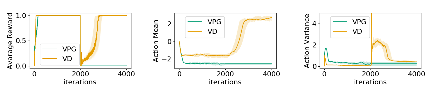
Figure 2: Average reward (left), action mean (middle), and variance (right) of the vanilla policy gradient (VPG) and our value dependent exploration (VD) on the continuous bandit example.

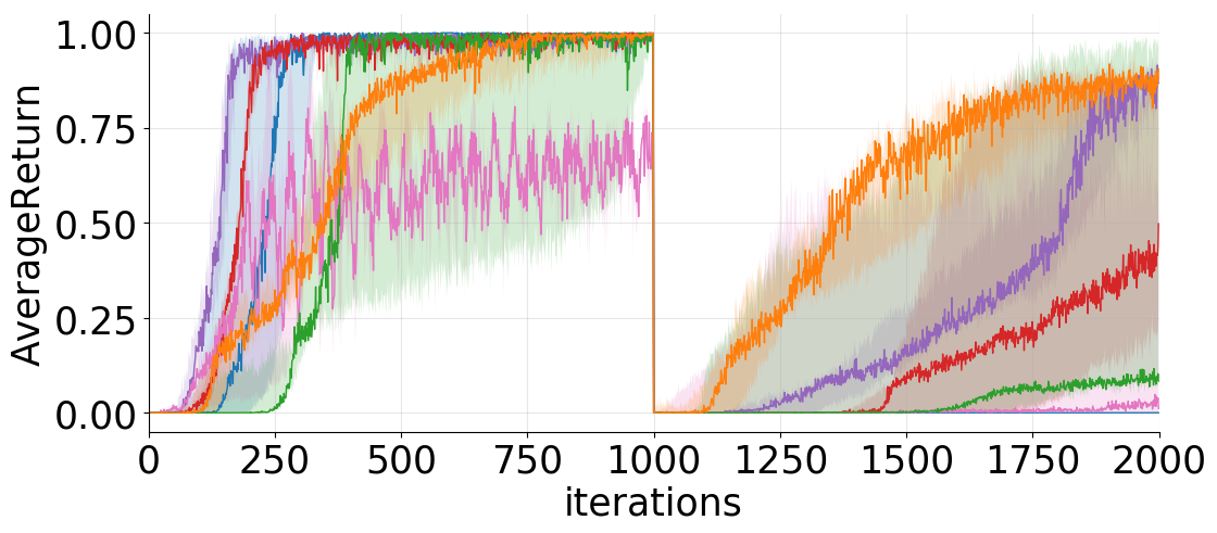
(a) DIP-center.

(b) Thrower.

(c) BiC.

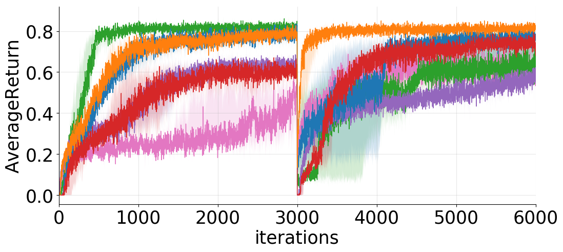
(d) Slide.

Figure 3: Learning curves on a variety environments and different environment changes.

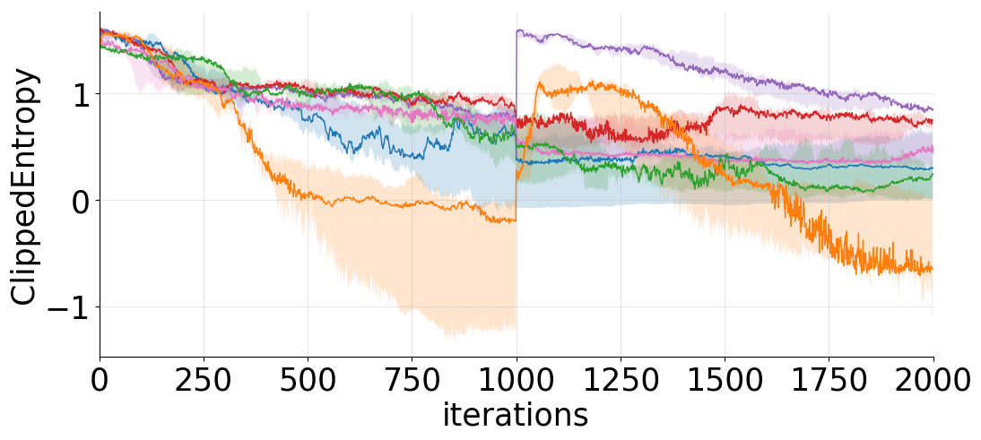
(a) DIP-center.

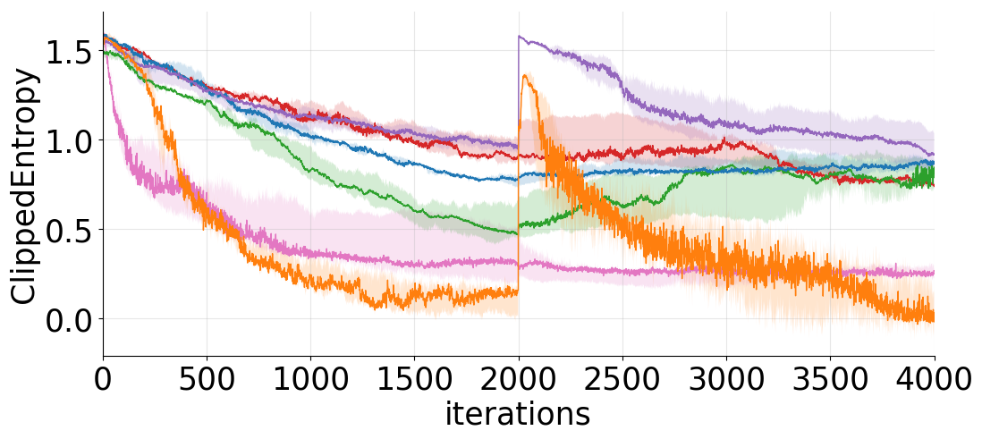
(b) Thrower.

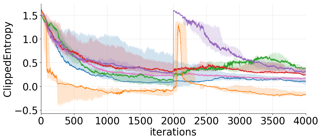
(c) BiC.

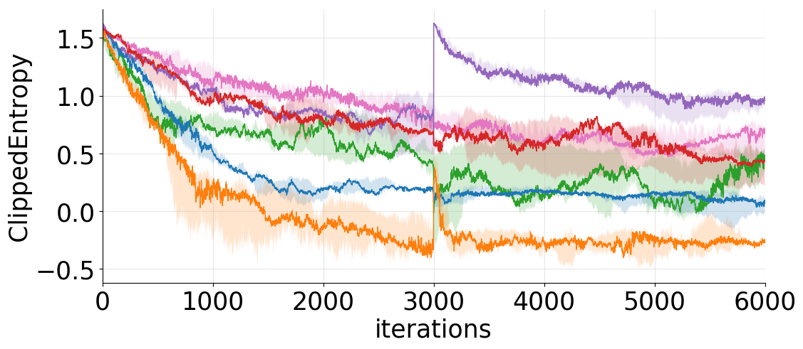
(d) Slide.

Figure 4: Average clipped entropy on a variety environments and different environment changes.

IV Evaluation

We evaluate our method on situations where there is a distribution shift in the environment. Specifically, the environments consist of two stages and there is a change in the environment parameters between the two stages, such as the position of objects, their orientation, or their center of mass (i.e. new objects that the agent encounters with a different mass distribution). In all our experiments, we plot the color band representing the 25 percentile and 75 percentile.

IV-A Continuous bandit example

We first test our method in a continuous bandit setting, with a one dimensional action space, which satisfies the assumptions stated in Section III-C. The reward is defined as

$$r_{t}(a)=\begin{cases}\mathds{1}\{a\in[-10,-1]\},&t\in[1,2000]\quad~{}~{}\text{(Stage I)}\\ \mathds{1}\{a\in[1,10]\},&t\in[2001,4000]\text{(Stage II)}\end{cases}$$

The policy is initialized as $a\sim\mathcal{N}(0,1)$. We compare two methods: 1) Vanilla policy gradient (REINFORCE [36]), where both the policy mean and variance are learned by gradient descent, and 2) Value dependent exploration, where the variance $\sigma_{i}=\frac{w}{\sqrt{2\pi e}\hat{V}_{i}}$, as suggested by Theorem 1. The parameter $w$ is learned by gradient descent. In both cases, the policy gradient update does not use a baseline function. We use ADAM [37] for adjusting the learning rate for both methods. The result is shown in Figure 2. We can see that before the environment changes at $t=2000$, both methods learn quickly, while the value dependent exploration decreases the variance faster to exploit better. When the environment changes, the vanilla policy gradient is not able to learn anymore due to the lack of positive reward and the limited exploration. On the other hand, the value dependent exploration quickly increases its variance when the value function drops, enabling the policy to receive positive rewards and learn much faster.

We provide further analysis on the convergence of the learned variance to the optimal variance in Appendix D, as well as the convergence of $w$ to the true value, showing that we can learn the optimal mapping from value to variance by gradient descent, despite the approximations.

IV-B Manipulation Environments

We further evaluate our method on complex manipulation tasks simulated in Mujoco [38]. We first specify a training iteration for the first stage so that all algorithms converge. Then we enter the second stage and change the environment in some way, without signaling the algorithms. We use TRPO for updating the policy mean. We use a policy modeled by a (32, 32) multi-layer perceptron (MLP) for all the algorithms. We have a value function $V_{discounted}$ with a discounted factor of 0.99 for baseline estimation, which is a (32, 32) MLP. The undiscounted value function $V_{\phi}$ that provides the input for our variance mapping function is of the same size. In all the experiments each dimension of the action space is normalized to $[-1,1]$ and the actions output by the policy are also clipped to be within this range.

For our value dependent exploration, we use a mapping function of the form:

$$\hat{\sigma}^{*}(s)=\frac{max(a,0)}{e^{k(V_{\phi}(s)-b)}+1}+max(c,0),$$ (4)

where $k,a,b,c$ are parameters that we can train with policy gradient updates. We denote this method as VD-Sigmoid (“VD" stands for “value dependent"). This function is guaranteed to be monotonically decreasing, as suggested by Theorem 2. However, this form is more flexible than the inverse function used for the continuous bandit case in Equation 3. Empirically, we found this parameterization of the mapping function performs well across the tasks. In all our experiments, the initial values of the parameters $k,a,b$, and $c$ are set to be $5,1.2,0.3$, and $0.1$ respectively. Examples of the learned variance mapping functions can be found in Appendix D.

Baselines We compare our method with four baselines which adjust the variance in different ways:

• Fixed variance: The variance is fixed to be $1$. This value was empirically determined to perform well, when the action is normalized to be in the range of $[-1,1]$.

• Global variance: The variance is defined as a global parameter, which is updated by policy gradient updates at each iteration, as was done in [31].

• State mapping: A neural network is learned to map each state to a variance, where the network is updated by policy gradient updates, as was done in [33].

• VIME [16]: VIME explores by maximizing the information gain computed by the posterior of a learned dynamics model.

• Relearn: Assume that drift detection [39] or context detection [29] is done perfectly, i.e. we know when the environment changes, a model is trained from scratch when the environment changes [39]. The baseline receives additional information of when the environment changes. We use a fixed variance for this baseline.

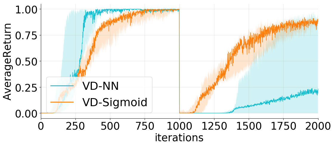
(a) DIP-center.

(b) Thrower.

(c) BiC.

(d) Slide.

Figure 5: Learning curves of value dependent exploration with different mapping functions. In all figures, the environment changes are the same with the corresponding experiments shown in Figure 3.

Evaluation Metric For each algorithm, we show its median return over 5 random seeds and plot this against the number of training iterations. To evaluate the amount of actual exploration of each method, we calculate the effective entropy of each policy after the action is clipped onto the range $[-1,1]$. Note that the variance by itself does not reveal the actual amount of exploration if the policy mean is much greater than 1 or much less than -1; due to the action clipping, the policy may be close to deterministic in these cases. The calculation of the entropy is given in Appendix C. A higher average entropy implies a higher degree of exploration. The clipped entropy is used only for evaluation and is not used for learning, as action-clipping is considered to be part of the environment and is unknown to the agent in the model-free setting that we are considering.

For all the environments, the learning curves and the corresponding entropy of policies learned by the different methods are plotted in Figures 3 and 4.

IV-B1 Environments details

Double inverted pendulum (DIP) In this environment, the task is to balance a double inverted pendulum.

Control 7 DOF Arm (Thrower) In this environment, we train a robot arm with 7 DOF to throw a ball into a basket. This environment is denoted as Thrower.

Ball in cup (BiC) A planar actuated cup can translate in order to swing and catch a ball attached via string. This environment is denoted as BiC.

Fetch slide object (Slide) In this environment, we train a Fetch robot to slide an object to the goal along a straight line.

All environments will change in its parameters during the half of the training. More environment details can be found in Appendix F.

IV-B2 Discussion

As shown in the plots in Figure 3, in stationary environments (before the environment changes), the value dependent exploration method performs about as well as the other baselines. However, when the environment changes, the average return of all methods drops at first, but the VD-Sigmoid recovers much faster. As seen from the entropy curves in Figure 4, the entropy of our method makes a very large jump quickly after the environment changes and then decreases again after the policy adapts. VIME performs as well as VD-Sigmoid in the BiC experiment, as the dynamics are relatively easy to learn. However, since VIME tries to systematically explore the dynamics for all of the observed state transitions, the environmental changes lead to unstable learning and often result in poor policy performance (as shown in Figures 3(a) and 3(b)), whereas our method leads to much more consistent policy improvements, both before and after environmental changes. The Relearn assumes knowledge of the changing point in the environment. However, re-training a model from scratch throws out all the past experiences and thus takes a longer time to learn in many cases. The fact the our model outperforms Relearn shows that past experience helps to learn new in new situations.

IV-C Comparison of different mapping functions

To see how much the monotonicity constraint (Theorem  2) helps, we compare the performance of our constrained mapping function VD-Sigmoid (Equation 4) to that of an unconstrained mapping function. For the unconstrained mapping function, we use $f_{\rho}\colon V_{\phi}(s)\mapsto\sigma$ modeled by a (4,4) multi-layer perceptron (MLP) with tanh as an activation function, trained with policy gradient updates, denoted as VD-NN. We compare the learning curves of VD-NN with the one that uses our constrained function in Figure 5. We can see that VD-NN has slower adaptation. The unconstrained neural network has a harder time learning an appropriate mapping function from the value to the action variance, because in high action dimensions, the relationship between the policy performance and the action variance of different action dimensions becomes complicated. The VD-Sigmoid adapts much faster than VD-NN, showing the importance of using a function that is constrained to be monotonically decreasing. Examples of the learned mapping functions are shown in the Appendix E.

V Future Work

Currently our method only deals with sparse-reward environments. A possible future direction is to extend our work to dense-reward environments, allowing the agent to optimally adapt its exploration in such settings. Since environmental changes are common in the real world, providing better exploration strategies for such cases will lead to more robust and wider application of robot learning.

VI Acknowledgement

This material is based upon work supported by the United States Air Force and DARPA under Contract No. FA8750-18-C-0092. The views and conclusions contained in this document are those of the author and should not be interpreted as representing the official policies, either expressed or implied, of any sponsoring institution, the U.S. government or any other entity.

References

- [1] J. Schulman, F. Wolski, P. Dhariwal, A. Radford, and O. Klimov, “Proximal policy optimization algorithms,” arXiv preprint arXiv:1707.06347, 2017.
- [2] M. C. R. J. B. M. J. P. A. P. M. P. G. P. A. R. J. S. S. S. J. T. P. W. L. W. W. Z. OpenAI: Marcin Andrychowicz, Bowen Baker, “Learning dexterous in-hand manipulation,” arXiv preprint arXiv:1808.00177, 2018.
- [3] A. Rajeswaran, V. Kumar, A. Gupta, J. Schulman, E. Todorov, and S. Levine, “Learning complex dexterous manipulation with deep reinforcement learning and demonstrations,” arXiv preprint arXiv:1709.10087, 2017.
- [4] D. Amodei, C. Olah, J. Steinhardt, P. Christiano, J. Schulman, and D. Mané, “Concrete problems in AI safety,” ArXiv preprint ArXiv:1606.06565, 2016.
- [5] Quionero-Candela, Joaquin and Sugiyama, Masashi and Schwaighofer, Anton and Lawrence, Neil D, Dataset Shift in Machine Learning. The MIT Press, 2009.
- [6] M. Sugiyama and M. Kawanabe, Machine learning in non-stationary environments: Introduction to covariate shift adaptation. MIT press, 2012.
- [7] N. Littlestone, “Learning quickly when irrelevant attributes abound: A new linear-threshold algorithm,” Machine learning, vol. 2, no. 4, pp. 285–318, 1988.
- [8] L. Yang, “Active learning with a drifting distribution,” in Advances in Neural Information Processing Systems 24, J. Shawe-Taylor, R. S. Zemel, P. L. Bartlett, F. Pereira, and K. Q. Weinberger, Eds. Curran Associates, Inc., 2011, pp. 2079–2087.
- [9] L. Li, M. L. Littman, and T. J. Walsh, “Knows what it knows: A framework for self-aware learning,” in Proceedings of the 25th International Conference on Machine Learning, ser. ICML ’08. New York, NY, USA: ACM, 2008, pp. 568–575.
- [10] I. Osband, C. Blundell, A. Pritzel, and B. Van Roy, “Deep exploration via bootstrapped DQN,” in Advances in Neural Information Processing Systems, D. D. Lee, M. Sugiyama, U. V. Luxburg, I. Guyon, and R. Garnett, Eds., 2016, pp. 4026–4034.
- [11] T. Haarnoja, H. Tang, P. Abbeel, and S. Levine, “Reinforcement learning with deep Energy-Based policies,” in International Conference on Machine Learning, 2017.
- [12] R. Fox, A. Pakman, and N. Tishby, “Taming the noise in reinforcement learning via soft updates,” in Conference on Uncertainty in Artificial Intelligence, 2016.
- [13] O. Nachum, M. Norouzi, K. Xu, and D. Schuurmans, “Bridging the gap between value and policy based reinforcement learning,” in Advances in Neural Information Processing Systems, 2017.
- [14] H. Tang, R. Houthooft, D. Foote, A. Stooke, X. Chen, Y. Duan, J. Schulman, F. De Turck, and P. Abbeel, “#exploration: A study of Count-Based exploration for deep reinforcement learning,” in Advances in Neural Information Processing Systems, 2017.
- [15] M. G. Bellemare, S. Srinivasan, G. Ostrovski, T. Schaul, D. Saxton, and R. Munos, “Unifying Count-Based exploration and intrinsic motivation,” in Advances in Neural Information Processing Systems, 2016.
- [16] R. Houthooft, X. Chen, Y. Duan, J. Schulman, F. De Turck, and P. Abbeel, “Curiosity-driven exploration in deep reinforcement learning via bayesian neural networks,” in Advances in Neural Information Processing Systems, 2016.
- [17] J. Achiam and S. Sastry, “Surprise-Based intrinsic motivation for deep reinforcement learning,” ArXiv preprint ArXiv:1703.0173, 2017.
- [18] B. O’Donoghue, I. Osband, R. Munos, and V. Mnih, “The uncertainty bellman equation and exploration,” ArXiv preprint ArXiv:1709.05380, 2017.
- [19] M. Tokic, “Adaptive -Greedy exploration in reinforcement learning based on value differences,” in KI 2010: Advances in Artificial Intelligence, ser. Lecture Notes in Computer Science. Springer, Berlin, Heidelberg, 2010, pp. 203–210.
- [20] A. Tamar, D. D. Castro, and S. Mannor, “Learning the variance of the reward-to-go,” Journal of Machine Learning Research, vol. 17, no. 13, pp. 1–36, 2016. [Online]. Available: http://jmlr.org/papers/v17/14-335.html
- [21] Y. Sakaguchi and M. Takano, “Reliability of internal prediction/estimation and its application. i. adaptive action selection reflecting reliability of value function,” Neural Networks, vol. 17, no. 7, pp. 935–952, 2004.
- [22] W. Yu, J. Tan, C. Karen Liu, and G. Turk, “Preparing for the unknown: Learning a universal policy with online system identification,” ArXiv prerpint ArXiv:1702.02453, 2017.
- [23] X. B. Peng, M. Andrychowicz, W. Zaremba, and P. Abbeel, “Sim-to-Real transfer of robotic control with dynamics randomization,” in IEEE International Conference on Robotics and Automation, 2018.
- [24] A. Rajeswaran, S. Ghotra, B. Ravindran, and S. Levine, “EPOpt: Learning robust neural network policies using model ensembles,” in International Conference on Learning Representations, 2016.
- [25] C. Finn, P. Abbeel, and S. Levine, “Model-Agnostic Meta-Learning for fast adaptation of deep networks,” in International Conference on Machine Learning, 2017.
- [26] Y. Duan, J. Schulman, X. Chen, P. L. Bartlett, I. Sutskever, and P. Abbeel, “RL2: Fast reinforcement learning via slow reinforcement learning,” ArXiv preprint ArXiv:1611.02779, 2016.
- [27] M. Al-Shedivat, T. Bansal, Y. Burda, I. Sutskever, I. Mordatch, and P. Abbeel, “Continuous adaptation via Meta-Learning in nonstationary and competitive environments,” in International Conference on Learning Representations, 2018.
- [28] S. P. Choi, D.-Y. Yeung, and N. L. Zhang, “Hidden-mode markov decision processes for nonstationary sequential decision making,” in Sequence Learning. Springer, 2000, pp. 264–287.
- [29] B. C. Da Silva, E. W. Basso, A. L. Bazzan, and P. M. Engel, “Dealing with non-stationary environments using context detection,” in Proceedings of the 23rd international conference on Machine learning. ACM, 2006, pp. 217–224.
- [30] V. Gullapalli, “A stochastic reinforcement learning algorithm for learning real-valued functions,” Neural networks, vol. 3, no. 6, pp. 671–692, 1990.
- [31] J. Schulman, S. Levine, P. Abbeel, M. Jordan, and P. Moritz, “Trust region policy optimization,” in International Conference on Machine Learning, 2015, pp. 1889–1897.
- [32] V. Mnih, A. P. Badia, M. Mirza, A. Graves, T. Lillicrap, T. Harley, D. Silver, and K. Kavukcuoglu, “Asynchronous methods for deep reinforcement learning,” in International Conference on Machine Learning, 2016, pp. 1928–1937.
- [33] T. Degris, P. M. Pilarski, and R. S. Sutton, “Model-free reinforcement learning with continuous action in practice,” in American Control Conference (ACC), 2012. IEEE, 2012, pp. 2177–2182.
- [34] R. Agrawal, “The continuum-armed bandit problem,” SIAM Journal on Control and Optimization, vol. 33, no. 6, pp. 1926–1951, 1995.
- [35] R. J. Hyndman, “Computing and graphing highest density regions,” The American Statistician, vol. 50, no. 2, pp. 120–126, 1996.
- [36] R. J. Williams, “Simple statistical gradient-following algorithms for connectionist reinforcement learning,” Machine Learning, vol. 8, no. 3-4, pp. 229–256, 1992.
- [37] D. P. Kingma and J. Ba, “Adam: A method for stochastic optimization,” arXiv preprint arXiv:1412.6980, 2014.
- [38] E. Todorov, T. Erez, and Y. Tassa, “Mujoco: A physics engine for model-based control,” in Intelligent Robots and Systems (IROS), 2012 IEEE/RSJ International Conference on. IEEE, 2012, pp. 5026–5033.
- [39] J. Gama, P. Medas, G. Castillo, and P. Rodrigues, “Learning with drift detection,” in Advances in Artificial Intelligence – SBIA 2004, ser. Lecture Notes in Computer Science. Springer, Berlin, Heidelberg, 2004, pp. 286–295.