Hyperspectral Image Classification with Deep Metric Learning and Conditional Random Field

Abstract

To improve the classification performance in the context of hyperspectral image processing, many works have been developed based on two common strategies, namely the spatial-spectral information integration and the utilization of neural networks. However, both strategies typically require more training data than the classical algorithms, aggregating the shortage of labeled samples. In this letter, we propose a novel framework that organically combines the spectrum-based deep metric learning model and the conditional random field algorithm. The deep metric learning model is supervised by the center loss to produce spectrum-based features that gather more tightly in Euclidean space within classes. The conditional random field with Gaussian edge potentials, which is firstly proposed for image segmentation tasks, is introduced to give the pixel-wise classification over the hyperspectral image by utilizing both the geographical distances between pixels and the Euclidean distances between the features produced by the deep metric learning model. The proposed framework is trained by spectral pixels at the deep metric learning stage and utilizes the half handcrafted spatial features at the conditional random field stage. This settlement alleviates the shortage of training data to some extent. Experiments on two real hyperspectral images demonstrate the advantages of the proposed method in terms of both classification accuracy and computation cost.

1 Introduction

Hyperspectral images (HSI) are usually acquired by spaceborne or airborne sensors, recording the reflection spectra or radiance spectra over hundreds of channels. They are usually formatted as data cubes. The height and width of an HSI data cube correspond to the real world object under a specific resolution, while the depth is decided by the channels of the sensors. As a crucial task, the classification of HSI pixels attracts great attention for a long time [1, 2, 3]. Many early methods are based on classical machine learning algorithms and their variations, for instance, principal component analysis (PCA) [4, 5], independent component analysis (ICA) [6], linear discriminant analysis (LDA) [7, 8], support vector machine (SVM) [9], and sparse representation [10, 11].

In recent years, neural networks (NN) have gained popularity in many applications related to machine learning, due to its power in generating abstract representations from the original data. An increasing number of NN-based algorithms have been adapted to HSI classification tasks and achieved impressive results. Representatives of the earlier models are stacked autoencoder (SAE) [12], and deep belief network (DBN) [13]. With the advances in deep learning, various deep models have been applied to HSI classification tasks, demonstrating their power in both processing spatial data and producing self-learned features. This category of algorithms mainly includes convolutional neural network (CNN) [14, 15, 16], recurrent neural network (RNN) [17, 18, 19], and deep metric learning (DML) [20, 21, 22], to name a few.

The conditional random field (CRF) is a probabilistic graphical algorithm that enables to characterize the contextual information among the labels and the data [23]. As an important application of CRF, image segmentation has also attracted attention in classifying HSI pixels [24, 25, 26, 27]. In most of these works, the CRFs were integrated sequentially after the CNNs as a post-processing step, processing the output features extracted by CNN encoders. For example, in [25], a restricted CRF algorithm is applied to refine the superpixel classification from a CNN to the final pixel-wise classification results. In [27], the authors utilized a CRF to improve the predictions on the CNN outputs and designed a specific deconvolutional network to produce the final classifications.

In this letter, a framework that combines the DML and CRF algorithms is proposed. The DML model supervised with center loss is employed to extract spectrum-based features from individual pixels. The CRF algorithm is applied to give final predictions by modeling both the spatial and spectral information from the spectrum-based features extracted by the DML model. To be more precise, our work has advantages in the following aspects:

• The intrinsic relations between DML and CRF help to improve the classification accuracies. To the best of our knowledge, we are the first to introduce a framework that benefits from the underlying connections between DML and CRF.

• The setting of employing a spectrum-based DML model and a handcraft spatial-based CRF algorithm keeps the framework simple. Compared to the CNN models, our framework is spectrum-based in the training phase and engages a simpler model structure, thus alleviating the shortage of labeled HSI data raised in the CNN models [15, 20].

• In practice, the proposed framework shows high efficiency in computation cost, for introducing the convolutional CRF (ConvCRF) [28], in which the CRF inferences are implemented on the GPU phase by convolutional operations.

2 Proposed Framework

As the two main parts of the proposed framework, DML and CRF algorithms are firstly introduced separately. Substantially, an overview of the whole DML-CRF framework is presented.

2.1 Deep Metric Learning

In [20], the center loss proposed in the deep metric learning model [29] was first introduced to the HSI classification tasks. A 3-layered fully connected network was built to extract spectral features from the input data. As illustrated in Fig. 1, the model is jointly supervised by cross-entropy loss (also called softmax loss) and center loss. Under this settlement, the extracted features from the same class gather more tightly in Euclidean space. This model is adopted to encode the spectrum in our work.

Throughout this letter, we use $(\mathbf{x}_{i},y_{i})$ to denote the pixel $\mathbf{x}_{i}$ with the label $y_{i}$, from the HSI $\mathbf{X}$. Let $f(\cdot)$ be the function defined by the neural network, whose values are the extracted features. Use $\tilde{p}(y|\mathbf{x}_{i})$ to denote the predicted probability distribution that is calculated by applying the softmax function on the extracted features $f(\mathbf{x}_{i})$. During the training stage, a joint loss $\mathcal{L}$ that sums the center loss $\mathcal{L}_{c}$ and the cross-entropy loss $\mathcal{L}_{s}$ is engaged. As the key part of DML, the center loss $\mathcal{L}_{c}$ is defined to measure the Euclidean distance between the produced features $f(\mathbf{x}_{i})$ and its class centers $\mathbf{c}_{y_{i}}$, as

$$\mathcal{L}_{c}=\sum_{i}||f(\mathbf{x}_{i})-\mathbf{c}_{y_{i}}||_{2},$$ (1)

where the class centers are formulated as

$$\mathbf{c}_{y_{i}}=\mathrm{average}(\{f(\mathbf{x}_{k})|\,y_{k}=y_{i}\}).$$

Figure 1: Structure of the spectral feature extraction network DML [20].

At the testing stage, samples $\mathbf{x}_{i}$ are fed to the neural network $f(\cdot)$. The outputs, which include both the extracted feature $f(\mathbf{X})$ and the predicted probability distribution $\tilde{p}(y|\mathbf{x}_{i})$, are collected for the subsequential CRF step.

2.2 Conditional Random Field

The CRF algorithm plays an important role in image segmentation, with the merit of exploiting the global context information [23, 30, 28]. In this letter, we use the CRF with Gaussian edge potentials to fuse the spatial-spectral information, and give reasonable pixel-wise predictions of the HSI. The notations in this letter mainly follow the models of fully connected CRF in [30] and ConvCRF in [28].

Let $\hat{y}$ be a choice of predictions over all the pixels in an HSI, the probability of $\hat{y}$ is calculated from an energy function $E(\hat{y}|f(\mathbf{X}))$ by a Gibbs distribution:

$$P(\hat{y}|f(\mathbf{X}))=\frac{\mathrm{exp}(-E(\hat{y}|f(\mathbf{X})))}{Z(f(\mathbf{X}))},$$

where $Z(f(\mathbf{X}))$ is the partition function [23]. In this algorithm, the energy function $E(\hat{y}|f(\mathbf{X}))$ is set to have two parts, with

$$E(\hat{y}|f(\mathbf{X}))=\sum_{i}\psi_{u}(\hat{y}_{i}|\mathbf{x}_{i})+\sum_{i<j}\psi_{p}(\hat{y}_{i},\hat{y}_{j}|\mathbf{x}_{i},\mathbf{x}_{j}),$$

where $\psi_{u}(\hat{y}_{i}|\mathbf{x}_{i})$ is the unary potential and $\psi_{p}(\hat{y}_{i},\hat{y}_{j}|\mathbf{x}_{i},\mathbf{x}_{j})$ is the pairwise potential. As in most applications of CRF, the unary potential is set to be the cost of a pixel $\mathbf{x}_{i}$ taking label $\hat{y}_{i}$, which is

$$\psi_{u}(\hat{y}_{i}|\mathbf{x}_{i})=-\mathrm{log}(\tilde{p}(\hat{y}_{i}|\mathbf{x}_{i})).$$ (2)

The pairwise potential is set to be

$$\psi_{p}(\hat{y}_{i},\hat{y}_{j}|\mathbf{x}_{i},\mathbf{x}_{j})=\mu(\hat{y}_{i},\hat{y}_{j})(w^{\mathrm{app}}k_{\mathrm{app}}+w^{\mathrm{smo}}k_{\mathrm{smo}}),$$ (3)

where $\mu(\hat{y}_{i},\hat{y}_{j})$ is called compatibility function and given by the Potts model $\mu(\hat{y}_{i},\hat{y}_{j})=|\hat{y}_{i}\neq\hat{y}_{j}|$, the $k_{\mathrm{app}}$ and $k_{\mathrm{smo}}$ are respectively termed the appearance and smooth kernels, and the $w^{\mathrm{app}}$ and $w^{\mathrm{smo}}$ are linear combination weights. If we denote the position of $\mathbf{x}_{i}$ as $p_{i}$, the appearance kernel $k_{\mathrm{app}}$ in (3) is defined as

$$k_{\mathrm{app}}(\hat{y}_{i},\hat{y}_{j}|\mathbf{x}_{i},\mathbf{x}_{j})$$ (4)

$$= \mathrm{exp}\left(-\frac{|p_{i}-p_{j}|^{2}}{2\theta_{\alpha}^{2}}-\frac{|f(\mathbf{x}_{i})-f(\mathbf{x}_{j})|^{2}}{2\theta_{\beta}^{2}}\right)$$

and the smoothness kernel $k_{\mathrm{smo}}$ is

$$k_{\mathrm{smo}}(\hat{y}_{i},\hat{y}_{j}|\mathbf{x}_{i},\mathbf{x}_{j})=\mathrm{exp}\left(-\frac{|p_{i}-p_{j}|^{2}}{2\theta_{\gamma}^{2}}\right).$$

As stated in [30], the appearance kernel is based on the observation that neighboring pixels with similar features tend to be from the same class, while the smoothness kernel helps to eliminate small isolated regions. It is noteworthy that the pairwise potential integrates both the spectral information and geographical information.

Mathematically, the final prediction is obtained by

$$y^{*}=\operatorname*{arg\,max}_{\hat{y}}P(\hat{y}|f(\mathbf{X})),$$

which is, however, hard to compute. Usually, a method of mean field approximation [30] is used to approximately calculate the results. In [28], the authors assumed that the pairwise potentials only take effect when the Manhattan distance between $\mathbf{x}_{i}$ and $\mathbf{x}_{j}$ is less than the so-called filter-size $k$. Under this assumption, the mean field inference algorithm could be implemented on the GPU phase and calculated more efficiently. This inference algorithm is called ConvCRF. Readers may refer [30, 28] for more detailed definitions and calculations of CRF.

2.3 A Summary

In general, we first use a DML model to generate spectrum-based features $f(\mathbf{x}_{i})$, as well as the preliminary predictions $\tilde{p}(y|\mathbf{x}_{i})$. Then, the preliminary predictions $\tilde{p}(y|\mathbf{x}_{i})$ are reformulated as the unary potentials of CRF by (2). The pairwise potentials, which include the appearance and smooth kernels, are expressed by (3) using features $f(\mathbf{x}_{i})$ and the corresponding pixels’ positions $p_{i}$. Finally, the ConvCRF algorithm is adopted to make CRF inference, producing the final predictions over all the pixels in an HSI.

In essence, it is the intrinsic connection between the center loss of DML and the appearance kernel of CRF that contributes to the performance of the proposed framework. Compared to the features extracted by the conventional NN models, the features extracted by DML with center loss gather more tightly in Euclidean space within the same class, i.e., pixels from the same class tend to be encoded as more similar features. Meanwhile, the appearance kernel (4) is designed to rely on the Euclidean distances between features $f(\mathbf{x}_{i})$. When compared to CRFs that rely on raw pixel spectra or features from plain NN models, the existence of center loss in DML rationalizes the CRF algorithm in our framework and enhance the final classification results.

3 Experiments

3.1 Datasets Description

The experiments are carried out on two well-known HSI datasets, namely the Pavia University scene and the Salinas scene collected by the ROSIS sensor and the AVRIS sensor, respectively. The Pavia University scene used in experiments has a size $(610,340,103)$ in $(\mathrm{Height},\mathrm{Width},\mathrm{Bands})$. The spatial resolution is $1.3\,\mathrm{m}$, while the band depth covers the wavelength from $0.43\,\mathrm{\mu m}$ to $0.86\,\mathrm{\mu m}$ with $12$ noisy and water absorption bands removed. Regarding the Salinas scene, the size of the image is $(512,217,204)$ after removing $20$ water absorption bands. The spatial resolution is $3.7\,\mathrm{m}$, and the spectra cover a bandwidth range from $0.4\,\mathrm{\mu m}$ to $2.5\,\mathrm{\mu m}$.

3.2 Experimental Settings and Results

To show the advantage of combining DML and CRF, contrast experiments are carried out by implementing DML, NN-CRF, and the proposed framework DML-CRF. Here, the only difference between the NN model and the DML model is the absence of center loss in the former. Moreover, two state-of-art methods, namely $3$D-CNN [15] and CSFF (DML-CSFF) [21] are also compared as baselines of HSI classification algorithms. Experiments are performed with deep learning platforms Caffe [31] and PyTorch [32], on a machine equipped with CPU of Intel Xeon E5-2660@2.6GHz and GPU of NVIDIA TitanX.

As for the DML model in DML and DML-CRF, the length of the extracted feature is set to be $\mathrm{len}(f(\mathbf{x_{i}}))=32$. The hyperparameters, such as learning rate, balance weight $\lambda$, and etc., are all chosen as their default values in the original paper [20]. Regarding the CRF algorithm in NN-CRF and DML-CRF, there are five parameters $w^{\mathrm{app}}$, $w^{\mathrm{smo}}$, $\theta_{\alpha}$, $\theta_{\beta}$, and $\theta_{\gamma}$. According to [30], the performances of CRF in terms of classificationy are relatively robust to these five parameters. Therefore, the default setting,

$$w^{\mathrm{app}}=10,\,w^{\mathrm{smo}}=3,\,\theta_{\alpha}=0.1,\,\theta_{\beta}=80,\,\theta_{\gamma}=3,$$

in [30, 28] are used directly. The only hyperparameter that needs to be set is the filter-size $k$ in ConvCRF, which is chosen as $k=7$ for Pavia University scene and $k=15$ for Salinas scene. An analysis of these variables is given in Section 3.3. The comparing methods $3$D-CNN and CSFF (DML-CSFF) are implemented by following their original papers  [15, 21].

If not otherwise specified, the training samples used in all the experiments follow the same preprocessing procedure. Each dataset is firstly normalized to have zero mean and unit variance. The training set is formed by randomly chosen $200$ pixels per class. For $3$D-CNN, $200$ HSI patches from each class are randomly chosen instead. To avoid overfitting effects, virtual samples are generated by the linear combinations of the pixels from the same class, with formula $\tilde{\mathbf{x}}=q\mathbf{x}_{1}+(1-q)\mathbf{x}_{2}.$ They are adopted in the training stages of all the aforementioned neural networks. The classification performances are evaluated by three metrics, namely overall accuracy (OA), average accuracy (AA), and the kappa coefficient ($\kappa$). Briefly, the metric OA is the percentage of correctly classified samples over all the testing samples, the metric AA is calculated by averaging the classification accuracies from each class, and the coefficient $\kappa$ measures the agreement between the predicted labels and groundtruth labels by the formula

$$\kappa=\frac{p_{o}-p_{e}}{1-p_{e}}.$$

In this formula, the notation $p_{o}$ represents the chance that the predicted label agrees with groundtruth label, which is the overall accuracy (OA), while $p_{e}$ is the hypothetical probability of chance agreement. Assume we have the predicted distribution which has chance $p_{p}(i)$ to output a predicted label $i$, and the groundtruth distribution which has chance $p_{g}(i)$ to output a groundtruth label $i$, $p_{e}$ is then calculated by

$$p_{e}=\sum_{i}p_{p}(i)p_{g}(i).$$

The classification results with mean and standard deviation over five runs are reported in TABLE 1. As shown in the first three columns, the absence of either DML or CRF deteriorates the classification accuracies. Compared to the state-of-the-art methods, the proposed DML-CRF still leads to comparable results. The proposed DML-CRF outperforms $3$D-CNN with a large margin on both datasets. When compared to CSFF, DML-CRF performs better in all the metrics on the Pavia University scene. On the Salinas scene, DML-CRF surpasses CSFF in terms of AA, but is slightly inferior to CSFF in terms of OA and $\kappa$. The testing times of the comparing methods are given in TABLE 2. We observe the DML-CRF is overwhelmingly faster than CSFF and several times faster than $3$D-CNN, thanks to the implementation of ConvCRF on GPU.

In the proposed DML-CRF framework, the parameters in the DML model are trained by spectral data, while the parameters in the CRF algorithm are set directly. Compared to the most of the spatial-spectral algorithms which use the HSI patches as training data, only the spectral data is engaged in the training of DML-CRF. This alleviates the shortage of HSI data in one sense. Also, the algorithm DML-CRF engages a simple and spectrum-based DML model, hence it has fewer parameters than the spatial-spectral algorithms which usually use multiple CNN layers as the model structure. Typically, a model with less trainable parameters tends to have less overfitting issues, therefore it performs better with insufficient training data. In this letter, the training datasets of DML-CRF and $3$D-CNN are set to have the same cardinalities. Comparison between the classification accuracies of DML-CRF and $3$D-CNN in TABLE 1 partially confirms our hypothesis mentioned above.

Table 1: Classification accuracies (averaged over 5 runs) of DML, NN-CRF, DML-CRF, $3$D-CNN, and CSFF on Pavia University scene and Salinas scene

		DML	NN-CRF	DML-CRF	$3$D-CNN	CSFF
Pavia Univ.	OA($\%$)	$93.67\pm 0.31$	$98.78\pm 0.15$	$99.10\pm 0.10$	$98.14\pm 0.10$	$98.90\pm 0.14$
	AA($\%$)	$93.64\pm 0.22$	$97.53\pm 0.18$	$98.72\pm 0.20$	$97.32\pm 0.68$	$98.49\pm 0.13$
	$\kappa$	$0.9153\pm 0.0041$	$98.38\pm 0.20$	$0.9880\pm 0.0014$	$0.9687\pm 0.0015$	$0.9852\pm 0.0018$
Salinas	OA($\%$)	$92.72\pm 0.44$	$97.86\pm 0.28$	$98.12\pm 0.21$	$95.91\pm 0.87$	$98.53\pm 0.34$
	AA($\%$)	$97.09\pm 0.16$	$99.25\pm 0.11$	$99.26\pm 0.08$	$98.79\pm 0.29$	$99.02\pm 0.20$
	$\kappa$	$0.9186\pm 0.0049$	$97.62\pm 0.31$	$0.9791\pm 0.0024$	$0.9480\pm 0.0108$	$0.9835\pm 0.0038$

Table 2: Comparison of testing time (in seconds)

	3D-CNN	CSFF	DML-CRF
Pavia Univ.	$50.94$	$1779.45$	$8.68$
Salinas	$45.69$	$5453.36$	$17.51$

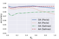
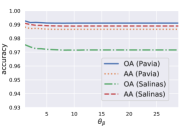
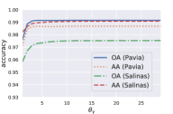
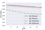
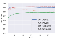
Figure 2: Classification accuracies in terms of AA and OA, along with varying parameters $w^{\mathrm{app}}$, $w^{\mathrm{smo}}$, $\theta_{\alpha}$, $\theta_{\beta}$, and $\theta_{\gamma}$, on Pavia University and Salinas scenes.

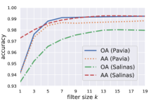
Figure 3: Classification accuracies in terms of AA and OA, along with varying hyperparameter $k$, on Pavia University and Salinas scenes.

3.3 Parameter Optimization

This subsection mainly discusses the effects of different choices of parameters and hyperparameters in CRF. For the hyperparameters in the DML model, details on their behaviors of them can be found in [20].

To verify the robustness of CRF to the parameters $w^{\mathrm{app}}$, $w^{\mathrm{smo}}$, $\theta_{\alpha}$, $\theta_{\beta}$, and $\theta_{\gamma}$, we anchor the default values by $w^{\mathrm{app}}=10,\,w^{\mathrm{smo}}=3,\,\theta_{\alpha}=0.1,\,\theta_{\beta}=80,\,\theta_{\gamma}=3$. Under this setting, we perform several experiments by varying every single parameter at one time. The relationships between the parameters and the classification performances are presented in Fig. 2. It is obvious that the classification performances are relatively robust to the parameters.

Regarding the only hyperparameter $k$, which is the filter-size in ConvCRF, it controls the size of the spatial information that CRF takes into account. The effect of $k$ on the classification accuracies are shown in Fig. 3. As expected, larger filter-sizes lead to higher accuracies, but also require more cost of computation.

4 Conclusion

In this letter, we proposed a framework that combines DML and CRF. The DML model is used to extract features from pixels of HSIs. The advantage of center loss reduces the Euclidean distances between the extracted features which share the same class label. Later, the CRF algorithm is applied to give predictions over the whole HSI by using both the extracted features and their position information. Contrast experiments demonstrated that the absence of either DML or CRF declines the classification performances. Moreover, the proposed framework provides comparable results to the state-of-art methods in both classification accuracies and computation cost. Additional experiments are performed to show the effects of varying parameters and hyperparameters on the classification accuracies.

References

- [1] D. Lu and Q. Weng, “A survey of image classification methods and techniques for improving classification performance,” International Journal of Remote Sensing, vol. 28, no. 5, pp. 823–870, 2007.
- [2] M. Fauvel, Y. Tarabalka, J. A. Benediktsson, J. Chanussot, and J. C. Tilton, “Advances in spectral-spatial classification of hyperspectral images,” Proceedings of the IEEE, vol. 101, no. 3, pp. 652–675, 2013.
- [3] W. Li, F. Feng, H. Li, and Q. Du, “Discriminant analysis-based dimension reduction for hyperspectral image classification: A survey of the most recent advances and an experimental comparison of different techniques,” IEEE Geoscience and Remote Sensing Magazine, vol. 6, no. 1, pp. 15–34, March 2018.
- [4] S. Prasad and L. M. Bruce, “Limitations of principal components analysis for hyperspectral target recognition,” IEEE Geoscience and Remote Sensing Letters, vol. 5, no. 4, pp. 625–629, Oct 2008.
- [5] J. Jiang, J. Ma, C. Chen, Z. Wang, Z. Cai, and L. Wang, “Superpca: A superpixelwise pca approach for unsupervised feature extraction of hyperspectral imagery,” IEEE Transactions on Geoscience and Remote Sensing, vol. 56, no. 8, pp. 4581–4593, Aug 2018.
- [6] A. Villa, J. A. Benediktsson, J. Chanussot, and C. Jutten, “Hyperspectral image classification with independent component discriminant analysis,” IEEE Transactions on Geoscience and Remote Sensing, vol. 49, no. 12, pp. 4865–4876, Dec. 2011.
- [7] T. V. Bandos, L. Bruzzone, and G. Camps-Valls, “Classification of hyperspectral images with regularized linear discriminant analysis,” IEEE Transactions on Geoscience and Remote Sensing, vol. 47, no. 3, pp. 862–873, Mar. 2009.
- [8] W. Li, S. Prasad, J. E. Fowler, and L. M. Bruce, “Locality-preserving dimensionality reduction and classification for hyperspectral image analysis,” IEEE Transactions on Geoscience and Remote Sensing, vol. 50, no. 4, pp. 1185–1198, April 2012.
- [9] F. Melgani and L. Bruzzone, “Classification of hyperspectral remote sensing images with support vector machines,” IEEE Transactions on Geoscience and Remote Sensing, vol. 42, no. 8, pp. 1778–1790, Aug. 2004.
- [10] Y. Chen, N. M. Nasrabadi, and T. D. Tran, “Hyperspectral image classification using dictionary-based sparse representation,” IEEE Transactions on Geoscience and Remote Sensing, vol. 49, no. 10, pp. 3973–3985, Oct. 2011.
- [11] L. Fang, S. Li, X. Kang, and J. A. Benediktsson, “Spectral-spatial hyperspectral image classification via multiscale adaptive sparse representation,” IEEE Transactions on Geoscience and Remote Sensing, vol. 52, no. 12, pp. 7738–7749, Dec. 2014.
- [12] Y. Chen, Z. Lin, X. Zhao, G. Wang, and Y. Gu, “Deep learning-based classification of hyperspectral data,” IEEE Journal of Selected Topics in Applied Earth Observations and Remote Sensing, vol. 7, no. 6, pp. 2094–2107, Jun. 2014.
- [13] Y. Chen, X. Zhao, and X. Jia, “Spectral-spatial classification of hyperspectral data based on deep belief network,” IEEE Journal of Selected Topics in Applied Earth Observations and Remote Sensing, vol. 8, no. 6, pp. 2381–2392, Jun. 2015.
- [14] V. Slavkovikj, S. Verstockt, W. De Neve, S. Van Hoecke, and R. Van de Walle, “Hyperspectral image classification with convolutional neural networks,” in Proceedings of the ACM international conference on Multimedia. ACM, 2015, pp. 1159–1162.
- [15] Y. Chen, H. Jiang, C. Li, X. Jia, and P. Ghamisi, “Deep feature extraction and classification of hyperspectral images based on convolutional neural networks,” IEEE Transactions on Geoscience and Remote Sensing, vol. 54, no. 10, pp. 6232–6251, Oct. 2016.
- [16] L. Jiao, M. Liang, H. Chen, S. Yang, H. Liu, and X. Cao, “Deep fully convolutional network-based spatial distribution prediction for hyperspectral image classification,” IEEE Transactions on Geoscience and Remote Sensing, vol. 55, no. 10, pp. 5585–5599, Oct. 2017.
- [17] L. Mou, P. Ghamisi, and X. X. Zhu, “Deep recurrent neural networks for hyperspectral image classification,” IEEE Transactions on Geoscience and Remote Sensing, vol. 55, no. 7, pp. 3639–3655, Apr. 2017.
- [18] Q. Liu, F. Zhou, R. Hang, and X. Yuan, “Bidirectional-convolutional lstm based spectral-spatial feature learning for hyperspectral image classification,” Remote Sensing, vol. 9, no. 12, 2017.
- [19] X. Zhang, Y. Sun, K. Jiang, C. Li, L. Jiao, and H. Zhou, “Spatial sequential recurrent neural network for hyperspectral image classification,” IEEE Journal of Selected Topics in Applied Earth Observations and Remote Sensing, vol. 11, no. 11, pp. 4141–4155, Nov 2018.
- [20] A. J. X. Guo and F. Zhu, “Spectral-spatial feature extraction and classification by ann supervised with center loss in hyperspectral imagery,” IEEE Transactions on Geoscience and Remote Sensing, vol. 57, no. 3, pp. 1755–1767, March 2019.
- [21] ——, “A cnn-based spatial feature fusion algorithm for hyperspectral imagery classification,” arXiv preprint arXiv:1801.10355, 2018.
- [22] G. Cheng, C. Yang, X. Yao, L. Guo, and J. Han, “When deep learning meets metric learning: Remote sensing image scene classification via learning discriminative cnns,” IEEE Transactions on Geoscience and Remote Sensing, vol. 56, no. 5, pp. 2811–2821, May 2018.
- [23] J. D. Lafferty, A. McCallum, and F. C. N. Pereira, “Conditional random fields: Probabilistic models for segmenting and labeling sequence data,” in Proceedings of the Eighteenth International Conference on Machine Learning, ser. ICML ’01. San Francisco, CA, USA: Morgan Kaufmann Publishers Inc., 2001, pp. 282–289.
- [24] F. I. Alam, J. Zhou, A. W. Liew, and X. Jia, “Crf learning with cnn features for hyperspectral image segmentation,” in 2016 IEEE International Geoscience and Remote Sensing Symposium (IGARSS), July 2016, pp. 6890–6893.
- [25] X. Pan and J. Zhao, “High-resolution remote sensing image classification method based on convolutional neural network and restricted conditional random field,” Remote Sensing, vol. 10, no. 6, 2018.
- [26] Z. Niu, W. Liu, J. Zhao, and G. Jiang, “Deeplab-based spatial feature extraction for hyperspectral image classification,” IEEE Geoscience and Remote Sensing Letters, vol. 16, no. 2, pp. 251–255, Feb 2019.
- [27] F. I. Alam, J. Zhou, A. W. Liew, X. Jia, J. Chanussot, and Y. Gao, “Conditional random field and deep feature learning for hyperspectral image classification,” IEEE Transactions on Geoscience and Remote Sensing, vol. 57, no. 3, pp. 1612–1628, March 2019.
- [28] M. T. Teichmann and R. Cipolla, “Convolutional crfs for semantic segmentation,” arXiv preprint arXiv:1805.04777, 2018.
- [29] Y. Wen, K. Zhang, Z. Li, and Y. Qiao, “A discriminative feature learning approach for deep face recognition,” in Proceedings of the European Conference on Computer Vision. Springer, 2016, pp. 499–515.
- [30] P. Krähenbühl and V. Koltun, “Efficient inference in fully connected crfs with gaussian edge potentials,” in Advances in neural information processing systems, 2011, pp. 109–117.
- [31] Y. Jia, E. Shelhamer, J. Donahue, S. Karayev, J. Long, R. Girshick, S. Guadarrama, and T. Darrell, “Caffe: Convolutional architecture for fast feature embedding,” in Proceedings of the ACM International Conference on Multimedia. ACM, 2014, pp. 675–678.
- [32] A. Paszke, S. Gross, S. Chintala, G. Chanan, E. Yang, Z. DeVito, Z. Lin, A. Desmaison, L. Antiga, and A. Lerer, “Automatic differentiation in pytorch,” in NIPS-W, 2017.