Learning Automata Based Q-learning for Content Placement in Cooperative Caching

Abstract

An optimization problem of content placement in wireless cooperative caching is formulated, with the aim of maximizing the sum mean opinion score (MOS) of mobile users. Firstly, as user mobility and content popularity has a significant impact on the system performance, a supervised feed-forward back-propagation connectionist model based neural network (SFBC-NN) is invoked for user mobility prediction and content popularity prediction. More particularly, practical data collected from GPS-tracker app on smartphones is tackled to test the accuracy of user mobility prediction. Then, based on the predicted mobile users’ positions and content popularity, a learning automata based Q-learning (LAQL) algorithm for wireless cooperative caching is proposed, in which learning automata (LA) is invoked for Q-learning to obtain an optimal action selection in a random and stationary environment. It is proven that the LA based action selection scheme is capable of enabling every state to select the optimal action with arbitrarily high probability if Q-learning is able to converge to the optimal Q value eventually. To characterize the performance of the proposed LAQL algorithms, sum MOS of users is applied to define the reward function. Extensive simulation results reveal that: 1) The prediction error of SFBC-NN based algorithm lessen with the increase of iterations and nodes; 2) the proposed LAQL achieves significant performance improvement against traditional Q-learning algorithm; and 3) the cooperative caching scheme is capable of outperforming non-cooperative caching and random caching of $3\%$ and $4\%$.

I Introduction

It is expected that the first fifth generation (5G)-network based solutions will be commercially launched by 2020 [2]. According to a recent report from Cisco [3], mobile data traffic has grown 18-fold over the past 5 years and will grow at a compound annual growth rate (CAGR) of 47 percent from 2016 to 2021. More particularly, mobile video traffic accounted for 60 percent of total mobile data traffic in 2016, and over three-fourths (78 percent) of the world s mobile data traffic will be video by 2021. In the vast area of 5G wireless systems, an extraordinary variety of technological innovations was included to support a large number of devices over limited spectrum resources [4, 5, 6]. Investigation presented in [7] shows that backhaul consumes up to 50 percent of the power in a wireless access network. Proactive caching at the base stations (BSs) is a promising approach to dealing with this problem, by introducing cache capabilities at BSs and then pre-fetching contents during off-peak hours before being requested locally by users (see [8], and references therein).

Designing proactive caching policy for each BS independently (e.g., each BS caching the most popular contents) may result in insufficient utilization of caching resources (see [9], and references therein). Cooperative caching increases content diversity in networks by exchanging availability information, thus further exploits the limited storage capacity and achieves more efficient wireless resource utilization (see [10, 11, 12, 13], and references therein). The key idea of cooperative caching is to comprehensively utilize the caching capacity of BSs to store specific contents, thus improving QoE of all users in networks. In [10], multicast-aware cooperative caching is developed using maximum distance separable (MDS) codes for minimizing the long-term average backhaul load. In [11], delay-optimal cooperative edge caching is explored, where a greedy content placement algorithm is proposed for reducing the average file transmission delay.

Based on aforementioned advantages of wireless caching, research efforts have been dedicated to caching solutions in wireless communication systems. Aiming to minimize the average downloading latency, the caching problem was formulated as an integer-linear programming problem in [14], which are solved by subgradient method. In [15], multi-hop cooperative caching is proposed for improving the success probability of content sharing [16]. The emerging machine learning paradigm, owing to its broader impact, has profoundly transformed our society, and it has been successfully applied in many applications [17], including playing Go games [18], playing atari [19], human-level control [20]. Wireless data traffic contains strong correlations and statistical features in various dimensions, thereby the application of machine learning in wireless cooperative caching networks optimization presents a novel perspective.

I-A Motivation and Related Works

Sparked by the aforementioned potential benefits, we therefore explore the potential performance enhancement brought by reinforcement learning for wireless cooperative caching networks. The authors in [21] proposed a context-aware proactive caching algorithm, which learns content popularity online by regularly observing context information of connected users. In [22], content caching is considered in a software-defined hyper-cellular networks (SD-HCN), aiming at minimizing the average content provisioning cost.

In[23], Q-learning based aerial base station (aerial-BS) assisted terrestrial network is considered to provides an effective placement strategy which increases the QoS of wireless networks. By integrating deep learning with Q-learning, deep Q-learning or deep Q-network (DQN) utilize a deep neural network with states as input and the estimated Q values as output, to efficiently learn policies for high-dimensional, large state-space problems [19]. In [24], an approach to perform proactive content caching was proposed based on the powerful frameworks of echo state networks (ESNs) and sublinear algorithms, which predicts the content popularity and users’ periodic mobility pattern. In [25], ESNs are used to effectively predict each user’s content request distribution and its mobility pattern when limited human-centric information such as users’ visited locations, requested contents, gender, job, and device type, etc.

Q-learning enables learning in an unknown environment as well as overcoming the prohibitive computational requirements, which has been widely used in wireless networks [26]. DQNs are used in [27] to solve a dynamic multichannel access problem. During peak hours, backhaul links become congested, which makes the QoE of end users low. One approach to mitigate this limitation is to shift the excess load from peak periods to off-peak periods. Caching realizes this shift by fetching popular contents, e.g., reusable video streams, during off peak periods, storing these contents in BSs equipped with memory units, and reusing them during peak traffic hours [28].

I-B Contributions and Organization

While the aforementioned research contributions have laid a solid foundation on wireless cooperative caching, the investigations on the applications of machine learning in wireless cooperative caching are still in their fancy [29]. In this article, we study the wireless cooperative caching system, where the caching capacity and the backhaul capacity are restricted. It is worth pointing out that the characteristics of cooperative caching make it challenging to apply the reinforcement learning, because the number of caching states increase exponentially with the number of contents and BSs. With the development of reinforcement learning and high computing speed of new computer, we design an autonomous agent, that perceives the environment, and the task of the agent is to learn from this non-direct and delayed payoff so as to maximize the cumulative effect of subsequent actions. The agent improves its performance and chooses behavior through learning.

Driven by solving all the aforementioned issues, we present a systematic approach for content cooperative caching. More specifically, we propose a learning automata based Q-learning (LAQL) algorithm for content placement in wireless cooperative caching networks (i.e., we consider “what” and “where” to cache). Instead of complex calculation of the optimal content placement, our designed algorithm enables a natural learning paradigm by state-action interaction with the environment it operates in, which can be used to mimic experienced operators. Our main contributions are summarized as follows.

1. We propose a content cooperative caching framework to improve QoE of users. We establish the correlation between user mobility, content popularity, and content placement in cooperative caching, by modeling the content placement with user mobility and content popularity. Then, we formulate the sum MOS maximization problem subject to the BSs’ caching capacity, which is a combinatorial optimization problem. We mathematically prove that the formulated problem is nondeterministic polynomial-time (NP) hard.

2. We invoke a supervised feed-forward back propagation connectionist models based neural network (SFBC-NN) for user mobility prediction and content popularity prediction. We explore the number of nodes and iterations of the SFBC-NN to improve the prediction accuracy. We utilize practical trajectory data collected from GPS-tracker app on smartphones to validate the accuracy of user mobility prediction.

3. We conceive an LAQL algorithm based solution for content placement in cooperative caching. In contrast to a conventional Q-learning algorithm, we design an action selection scheme invoking learning automata (LA). Additionally, we prove that the LA based action selection scheme is capable of enabling every state to select the optimal action with arbitrary high probability if Q-learning is capable of converging to the optimal Q value eventually.

4. We demonstrate that the performance of the proposed LAQL based content cooperative caching with content popularity and user mobility prediction outperforms conventional Q-learning. Meanwhile content cooperative caching is capable of outperforming non-cooperative caching and random caching algorithm in terms of QoE of users.

The rest of the paper is organized as follows. In Section II, the system model for content caching in different BSs is presented. In Section III, the SFBC-NN based user mobility and content popularity prediction are investigated. LAQL for content cooperative caching is formulated in Section IV. Simulation results are presented in Section V, before we conclude this work in Section VI. Table I provides a summary of the notations used in this paper.

TABLE I: LIST OF NOTATIONS

Notation	Description	Notation	Description
$M$	The number of BSs	$R_{m\min}$	The minimum fronthaul capacity of BS $m$
$N_{u}$	The number of users	${\rm{MO}}{{\rm{S}}_{i}}(t)$	The mean opinion score of user $i$ at time $t$
$F$	The umber of contents	${\rm RTT}$	The round trip time
$l\left({}\right)$	The size of content	${\rm FS}$	The web page size
${z_{i}}$	Position of user $i$	${\rm MSS}$	The maximum segment size
${z_{m}}$	Position of BS $m$	$L$	The number of slow start cycles with idle periods
${s_{m}}$	Caching capacity of BS $m$	${x_{l-1}^{input}}$	The input of layer $l-1$
${X_{m}}$	Caching vector of BS $m$	${{W^{l}}}$	The weights of layer $l$
${r_{mi}}$	Distance between user $i$ and BS $m$	${{b^{l}}}$	The bias of layer $l$
$\rho$	Transmit power of BSs	${{y^{output}}}$	The output of the network
${{h_{mi}}}$	Small scale fading of BS $m$ and user $i$	${{y^{real}}}$	The real data
${{\sigma^{2}}}$	The power of the additive noise	${Q^{\pi}}\left({s,a}\right)$	The Q table
${{I_{i}}}$	The sum of interfering signal power	${Q^{*}}\left({s,a}\right)$	The optimal state-action value function
$B$	The bandwidth of each downlink user	${u_{i}}\left(t\right)$	The times action $i$ has been rewarded when selected
${{p_{t,f}}}$	The popularity of content $f$ at time $t$	${v_{i}}\left(t\right)$	The number of times that action $i$ has been selected
$R_{m\max}$	The maximum fronthaul capacity of BS $m$	${P_{a}}\left(t\right)$	The probability distribution of LA

II System Model

II-A System Description

We consider a square cooperative area composed of $M$ base stations (BSs) with one transmit antennas and $N_{u}$ single antenna users (as is shown in Fig. 1). The central processor collects relevant information from the system, and acts as a master to control the BS (slaves), and implements a centrally controlled adjustment of caching policies [30]. Denote $\mathcal{M}=\left\{{1,\cdots,M}\right\}$ and $\mathcal{N}=\left\{{1,\cdots,N_{u}}\right\}$ be the BSs set and the user set, respectively. We assume that the content library in the central network consists of $F$ contents denoted by $\mathcal{F}=\left\{{1,\cdots,F}\right\}$, and the size of $f$-th content is $l\left(f\right)$. The position of user $i$ is denoted as $z_{i}$. The position of BS $m$ is denoted by $z_{m}$, and the caching capacity of BS $m$ is $s_{m}$. The content cache vector of BS $m$ is ${X_{m}}=\left[{{x_{1,m}},{x_{2,m}}\cdots,{x_{{s_{m}},m}}}\right]$, where ${x_{i,m}}\in\left[{1,F}\right]$. Therefore, the cooperative caching matrix is denoted as:

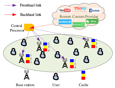
Figure 1: Schematic of the wireless cooperative caching scenario. The users are served by BSs cooperatively, and the contents cached in different BSs (slaves) are placed by cental processor (master).

$$X=\left[{\begin{array}[]{*{20}{c}}{{X_{1}}}\\ {{X_{2}}}\\ \vdots\\ {{X_{M}}}\end{array}}\right]=\left[{\begin{array}[]{*{20}{c}}{{x_{1,1}},{x_{2,1}}\cdots,{x_{{s_{1}},1}}}\\ {{x_{1,2}},{x_{2,2}}\cdots,{x_{{s_{2}},2}}}\\ \vdots\\ {{x_{1,M}},{x_{2,M}}\cdots,{x_{{s_{M}},M}}}\end{array}}\right].$$ (1)

We set the position of users randomly, and the position of user $i$ is denoted by ${z_{i}}=\left({{x_{i}},{y_{i}}}\right)$, and the position of BS $m$ is denote by ${z_{m}}=\left({{x_{m}},{y_{m}}}\right)$. As such, the distance from user $i$ to BS $m$ is given by $\left\|{{r_{mi}}}\right\|=\left\|{{z_{i}}-{z_{m}}}\right\|=\sqrt{{{\left({{x_{i}}-{x_{m}}}\right)}^{2}}+{{\left({{y_{i}}-{y_{m}}}\right)}^{2}}}$. We consider a wireless communication system with FDMA.

Consider content $f$ in the cooperative region, which is cached in multiple BSs, denoted by $\mathcal{M}_{f}$. These BSs jointly transmit content $f$ to user $i$ who requests for it. The received signal-interference-noise ratio (SINR) of received signal of user $i$ requesting for content $f$ is given by

$${\rm{SIN}}{{\rm{R}}_{mi}}=\frac{{{{\left({\sum\limits_{m\in\left\{{{\mathcal{M}_{f}}}\right\}}{\sqrt{\rho}\left|{{h_{mi}}}\right|r_{mi}^{-\alpha/2}}}\right)}^{2}}}}{{{I_{i}}+{\sigma^{2}}}},$$ (2)

where ${\rho}$ denotes the equally transmit power of all BSs, and ${\left|{{r_{mi}}}\right|^{-\alpha}}$ represents a standard distance-dependent power law pathloss attenuation between BS $m$ and user $i$, where $\alpha\geq 2$ is the pathloss exponent. ${h_{mi}}$ denotes the small-scale Rayleigh fading between BS $m$ and user $i$, ${{\sigma^{2}}}$ denotes the power of the additive noise and $I_{i}$ is the sum of interfering signal power from BSs that do not cache content $f$ given by

$${I_{i}}={\sum_{n\in\left\{\mathcal{M}\right\}\backslash\left\{{{\mathcal{M}_{f}}}\right\}}}\rho{\left|{{h_{ni}}}\right|^{2}}r_{ni}^{-\alpha},$$ (3)

The bandwidth of each downlink user is denoted as $B$, Therefore, based on Shannon’s capacity formula, the overall achievable sum rate of user $i$ at time $t$ can be expressed as

$${R_{t,i}}=B\sum\limits_{f=1}^{F}{\left({{p_{t,f}}\sum\limits_{m=1}^{M}{{x_{t,mf}}{{\log}_{2}}\left({1+SIN{R_{t,im}}}\right)}}\right)}.$$ (4)

where $p_{t,if}$ denotes content $f$’s popularity at time $t$.

If the content is not cached in the BS, then the content needs to be fetched from the centre network using fronthaul link. Due to the fronthaul link capacity constrains, the total transmitting rate of each BS should not exceed its fronthaul capacity $R_{m\max}$. Assuming there are $H_{m}$ users associated with BS $m$, thus

$$B\sum\limits_{i=1}^{{H_{m}}}{\left({{p_{t,mi}}{x_{t,mf}}{{\log}_{2}}\left({1+SIN{R_{t,im}}}\right)}\right)}\leq{R_{m\max}}.$$ (5)

Another constrain is that the transmit rate for each user should not be less than the minimum transmit rate ${R_{i\min}}$, thus

$$\sum\limits_{m=1}^{M}{\left({{p_{t,mi}}{x_{t,mf}}{{\log}_{2}}\left({1+SIN{R_{t,im}}}\right)}\right)}\geq{R_{i\min}}.$$ (6)

II-B Quality-of-Experience Model

As in [31], the definition of quality-of-experience (QoE) is “The overall acceptability of an application or service, as perceived subjectively by the end user.” the QoE is a kind of users’ satisfaction description during the process of interactions between users and services [32]. Based on [33], we define our MOS of user $i$ in time $t$ as

$${\rm{MO}}{{\rm{S}}_{i}}(t)=-{C_{1}}\ln\left({d\left({{R_{t,i}}}\right)}\right)+{C_{2}},$$ (7)

where $C_{1}$ and $C_{2}$ are constants determined by analyzing the experimental results of the web browsing applicants, which are set to be 1.120 and 4.6746, respectively. ${\rm{MO}}{{\rm{S}}_{i}}(t)$ represents the user perceived quality expressed in real numbers ranging from 1 to 5 (i.e., the score 1 represents extremely low quality, whereas score 5 represents excellent quality. $R_{t,i}$ is achievable sum rate of user $i$ at time $t$, and ${d\left({{R_{t,i}}}\right)}$ is the delay time of a user receiving a content. According to  [34],

$${d\left({{R_{t,i}}}\right)=3{\rm{RTT}}+\frac{{{\rm{FS}}}}{{{R_{t,i}}}}+L\left({\frac{{{\rm{MSS}}}}{{{R_{t,i}}}}+{\rm{RTT}}}\right)-\frac{{2{\rm{MSS}}\left({{{\rm{2}}^{\rm{L}}}{\rm{-1}}}\right)}}{{{R_{t,i}}}}},$$ (8)

where ${R_{t,i}}$ represents the data rate, ${\rm RTT}$ is the round trip time, ${\rm FS}$ is the web page size, and ${\rm MSS}$ is the maximum segment size. $L$ is the number of slow start cycles with idle periods, $L=\min\left[{{L_{1}},{L_{2}}}\right]$, which is defined as [34]: ${L_{1}}={\log_{2}}\left({\frac{{{R_{t,i}}{\rm{RTT}}}}{{{\rm{MSS}}}}+1}\right)-1$, ${L_{2}}=\log_{2}\left({\frac{{{\rm FS}}}{{2{\rm MSS}}}+1}\right)-1$, where $L_{1}$ denotes the number of cycles that the congestion window takes to reach the bandwidth-delay product and $L_{2}$ is the number of slow start cycles before the webpage size is completely transferred.

Substituting (8) into (7), we obtain MOS of user $i$ as follows:

$${\rm{MO}}{{\rm{S}}_{i}}(t)=-{C_{1}}\ln\left[{3{\rm{RTT}}+\frac{{{\rm{FS}}}}{{{R_{t,i}}}}\left.{+L\left({\frac{{{\rm{MSS}}}}{{{R_{t,i}}}}+{\rm{RTT}}}\right)-\frac{{2{\rm{MSS}}\left({{{\rm{2}}^{L}}{\rm{-1}}}\right)}}{{{R_{t,i}}}}}\right]+{C_{2}}.}\right.$$ (9)

III SFBC-NN Based User Mobility and Content Popularity Prediction

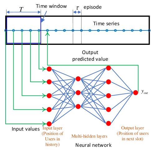
Figure 2: Flow chart of the SFBC-NN for time series prediction.

In reality, users are mobile, and may have periodic mobility patterns. We assume that the time interval of the change of users’ mobility is $T$. Universal approximation theorems in [35] show that neural networks have a striking fact that they compute any function at all. Hencefore in this section, we propose an SFBC-NN based user position and content popularity prediction algorithm. The structure of the SFBC-NN for user mobility prediction contains two hidden layers and a fully connected output layer. The inputs are users’ positions in one hour containing 12 positions.

Definition 1.

The definition of three parameters adopted in SFBC-NN are given below.

• Input layer (IL): Passive layer, receiving single value of input, and duplicating the value to multiple outputs. ${x_{t,i}}$ represents the position of the $i$-th user at time $t$, and the network input is the history combination of $M$ positions, i.e., $x^{input}=\left[{{x_{t-M,i}},{x_{t-M+1,i}},\cdots,{x_{t-1,i}}}\right]$. Here we set $M=12$ which means that we use history one hour positions to predict positions in the next hour.

• Output Layer (OL): Active layer, modifying the data of input, and exporting given outputs for the network. $y^{output}=\left[{{y_{t+1,i}},{y_{t+2,i}},\cdots,{y_{t+N,i}}}\right]$ represents the positions of the $i$-th user for the next step, where $N$ represents length of the track.

• Root mean square error (RMSE): The performance of the SFBC-NN based user mobility prediction developed in our work is evaluated by RMSE, which adjusts the weight of the network after each iteration, thus it affects the rate of convergence. The SFBC-NN produces a function relation between input ${I_{t,if}}$ and output ${O_{t,if}}$:

  $$y_{l}^{output}=f\left({{W^{l}}x_{l-1}^{input}+{b^{l}}}\right),$$ (10)

  where $W^{l}$ denotes the weight matrix of layer $l$, and $b^{l}$ denotes the bias of layer $l$. $f\left(\bullet\right)$ is the activation function (i.e., Sigmoid Function.), which is applied to node inputs to produce node output. The forward propagation algorithm will pass the information through the network to make a prediction in the output layer. After forward propagation, as in Definition 1, the network uses a RMSE function to measure the loss between trained output and output:

  $${\rm RMSE}\left({{y^{output}},{y^{real}}}\right)=\frac{1}{{{N_{u}}}}\sum\limits_{i=1}^{{N_{u}}}{\sqrt{\frac{1}{{{N_{o}}}}\sum\limits_{j=1}^{{N_{o}}}{{{\left[{y_{i}^{output}\left(j\right)-y_{i}^{real}\left(j\right)}\right]}^{2}}}}},$$ (11)

  where ${{y^{output}}}$ and ${{y^{real}}}$ denotes the output of the network and real data, respectively. The details of SFBC-NN based user mobility prediction are shown in Algorithm 1.

A typical SFBC-NN architecture contains input (denoted by $X_{t}$), the hidden layers ($H$), and output layers (denoted by $Y$). In our SFBC-NN, we desire a double hidden layers SFBC-NN to predict user mobility.

Algorithm 1 The SFBC-NN for user mobility prediction.

1:  Stage One: Training

1:  Time interval $H$, training data: positions of users $\left[{{x_{t-H+1,i}},{x_{t-H+2,i}},\cdots,{x_{t,i}}}\right]$. Parameters of SFBC-NN: number of hidden layers 2, learning rate 0.1, goal of RMSE, the number of epochs.

2:  Randomly initialize number of hidden layers, the weight matrix $W^{l}$ and the bias $b^{l}$.

3:  for each episode do

4:     Choose input $I_{t,if}$ from training set; 

5:     Forward propagation algorithm: calculating the output of the layers ${O^{l}}(l=1:{N_{ne}})$; 

6:     Calculate loss function $los{s^{l}}(l=1:{N_{ne}})$; 

7:     Backward propagation algorithm: adjust the weights ${W^{l}}(l=1:{N_{ne}})$ and bias ${b^{l}}(l=1:{N_{ne}})$ according to the loss function; 

8:  end for

8:  Weights ${W^{l}}(l=1:{N_{ne}})$ and bias ${b^{l}}(l=1:{N_{ne}})$ of the network. 

9:  Stage Two: Testing

9:  Interval $H$, Testing data: Positions of users, Parameters of SFBC-NN: weights ${W^{l}}(l=1:{N_{ne}})$, bias ${b^{l}}(l=1:{N_{ne}})$ of the network, the number of epochs.

10:  for each episode do

11:     Choose input $I_{t,if}$ from testing set; 

12:     Forward propagation: calculating the output of the layers ${O^{l}}(l=1:{N_{ne}})$; 

13:     Calculate loss function $los{s^{l}}(l=1:{N_{ne}})$; 

14:  end for

14:  The accuracy between predicted user’s positions and real data.

III-A Convergence of SFBC-NN

We obtain local optimal solution with gradient method training. Better training algorithms for SFBC-NN is needed to obtain global optimal solution, because it is more representationally efficient than shallow ones [36].

Remark 1.

For SFBC-NN based user mobility prediction, layer-wise pre-training (LWPT) is generally adopted, which means that in the beginning of the whole network, only a small number of separate neurons need to be trained, then the whole network is trained by gradient. In each step, we fix the pre-trained $k-1$ layers and add the $k$-th layer (that is, the input of $k$-th layer is the output of the former $k-1$ layers that we have trained). Each level of training is supervised (i.e., taking the prediction error of each step as the loss function).

III-B Stability of SFBC-NN

The stability of SFBC-NN with respect to small perturbations of the inputs is meaningful, because small perturbations like users’ unfrequent visit positions and abnormal contents surfing are not main concern in our scenario. We focus on scenarios that people periodical visit and contents that they request stably in the areas.

Remark 2.

Results suggest that the SFBC-NN for user mobility prediction that are learned by backpropagation have nonintuitive characteristics and intrinsic blind spots, and its structure is connected to the data distribution in a non-obvious way [37]. Thus in our scenario, data preprocessing (i.e., perturbations elimination) is of great importance to increase the stability of SFBC-NN based user mobility prediction.

Remark 3.

An apparent advantage of utilizing the SFBC-NN for content popularity prediction is that it stores the non-linear characters in the multi-parameters of SFBC-NN, which reflects the nature of the relationship between the inputs and the outputs.

In (4), content popularity $p_{t,mi}$ plays an important role in overall achievable sum rate, therefor content popularity is another element that we predict for content cooperative caching. Note that the dimension of content popularity is larger than user mobility. For this reason, we set more hidden layers than user mobility prediction network. The structure of the neural network based content popularity prediction contains three hidden layers and a fully connected output layer. The input data is partitioned into blocks of size ${k_{in}}=5\times 1$, where each block represents for content popularity in 5 time slots ${X_{in}}=\left[{{p_{ik}},\cdots,{p_{i(k+4)}}}\right]{\kern 1.0pt}{\kern 1.0pt}{\kern 1.0pt}{\kern 1.0pt}{\kern 1.0pt}{\kern 1.0pt}{\kern 1.0pt}{\kern 1.0pt}{\kern 1.0pt}{\kern 1.0pt}{\kern 1.0pt}{\kern 1.0pt}(k=1,2,\cdots)$. The output is a block of size ${k_{out}}=1\times 1$, where each block represents the content popularity in the next time slot ${Y_{out}}={p_{i(k+5)}}{\kern 1.0pt}{\kern 1.0pt}{\kern 1.0pt}{\kern 1.0pt}{\kern 1.0pt}{\kern 1.0pt}{\kern 1.0pt}{\kern 1.0pt}{\kern 1.0pt}(k=1,2,\cdots)$.

IV Learning Automata based Q-Learning for Content Cooperative Caching

IV-A Problem Formulation

We obtain users mobility and content popularity from Section III. Hereafter, the objective is to maximize the overall ${\rm{MO}}{{\rm{S}}_{tot}}(t)=\sum\limits_{u=1}^{N}{{\rm{MO}}{{\rm{S}}_{u}}(t)}$ with constrains from content cache vector X, content characteristics, and caching capacity of BSs. Let ${G_{t,mf}}={x_{t,mf}}{\log_{2}}\left({1+\rm{SIN{R}_{t,im}}}\right)$ for similarity. The content caching problem is to determine the cached data files’ distribution for each BS aiming to maximize the MOS of users, subject to the cache capacity constraint. The optimization problem is formally expressed as

$$\left(\textbf{{P1}}\right)\mathop{{\rm{max}}}\limits_{\textbf{X}}{\rm{MO}}{{\rm{S}}_{tot}}\left(t\right)=\sum\limits_{i=1}^{N}{{\rm{MO}}{{\rm{S}}_{i}}\left(t\right)},$$ (12a)

s.t. $$C_{1}:\;{x_{t,mf}}\in\left\{{0,1}\right\},\forall f\in F,m\in M,$$ (12b)

$$C_{2}:\;\sum\limits_{f=1}^{F}{{x_{t,mf}}{l_{f}}}\leq{S_{m}},\forall t\in T,m\in M,$$ (12c)

$$C_{3}:\;{p_{t,if}}\in\left({0,1}\right),\forall f\in F,i\in N_{u},$$ (12d)

$$C_{4}:\;\sum\limits_{m=1}^{M}{{s_{m}}}\leq\sum\limits_{f=1}^{F}{{l_{f}}},$$ (12e)

$$C_{5}:\;\sum\limits_{i=1}^{{H_{m}}}{B\left({{p_{t,mi}}{G_{t,mf}}}\right)}\leq{R_{m\max}},\forall t\in T,$$ (12f)

$$C_{6}:\;\sum\limits_{m=1}^{M}{\left({{p_{t,mi}}\sum\limits_{m=1}^{M}{{G_{t,mf}}}}\right)}\geq{R_{i\min}},\forall t\in T,$$ (12g)

where ${x_{t,mf}}$ denotes the caching decision of BS $m$ and content $f$ at time $t$, ${p_{t,if}}$ denotes the popularity of user $i$ for content $f$ at time $t$, and $N_{u}$ denotes the number of users. (12c) states that the total size of contents cached in BS $m$ should not exceed the content caching capacity of the BS. For simplicity, we assume that each content has the same size 1, i.e., ${l_{f}}=1$. This assumption is easily found by dividing contents into blocks with the same size [38]. (12e) ensures that the total caching capacity of all BSs is smaller than the total size of contents, otherwise the BSs would cache all the contents and the research is not meaningful. (12f) and (12g) are BS fronthaul link capacity constrain and user minimum transmit rate constrain, respectively.

Lemma 1.

The optimization problem in (12) is a NP-hard problem.

Proof:

See Appendix A . ∎

As indicated by Lemma 1, the problem is NP-hard and therefore the problem has no polynomial-time solution discovered so far. Instead of utilizing conventional optimization approaches, we formulate the problem as a finite Markov decision process (MDP), hereafter, we utilize Q-learning algorithm to solve the problem. In order to improve the performance of Q-learning, we adopt learning automata (LA) for the action selection of every state in Q-learning. We apply the predicted results of user mobility and content popularity from the proposed SFBC-NN algorithm in Section III as inputs for solving problem in (12). User position in (2) and content popularity in (4) are predicted by neural network, therefor the solution for (12) is content caching matrix.

IV-B Q-learning Based Solution

Q-learning is an off-policy and model-free reinforcement learning algorithm compared to policy iteration and value iteration. Moreover, the agent of Q-learning does not need to traverse all states and actions on contrary to value iteration. Q-learning stores state and action information into a Q table ${Q^{\pi}}\left({s,a}\right)$, where $\pi$ is the policy, $s$ represents the state, and $a$ represents the action. The objective of the Q-learning is to find optimal policy ${\pi^{*}}$, and estimate the optimal state-action value function ${Q^{*}}\left({s,a}\right):={Q^{\pi}}\left({s,a}\right),\forall s,a$, which can be shown that [39]

$${\pi^{*}}\left(s\right)=\mathop{\arg\max}\limits_{{\kern 1.0pt}{\kern 1.0pt}{\kern 1.0pt}{\kern 1.0pt}{\kern 1.0pt}{\kern 1.0pt}{\kern 1.0pt}{\kern 1.0pt}{\kern 1.0pt}{\kern 1.0pt}{\kern 1.0pt}{\kern 1.0pt}{\kern 1.0pt}{\kern 1.0pt}{\kern 1.0pt}{\kern 1.0pt}{\kern 1.0pt}{\kern 1.0pt}{\kern 1.0pt}{\kern 1.0pt}a}{Q^{*}}\left({s,a}\right),\forall s\in S,$$ (13)

where ${\pi^{*}}\left(s\right)$ denotes the optimal policy of state $s$, and $S$ denotes the set of all states.

The expression for optimal strategy ${V_{{\pi^{*}}}}\left(s\right)$ is rewritten as

$${V_{{\pi^{*}}}}\left(s\right)=\mathop{\max}\limits_{a\in A}\left[{r\left({s,a}\right)+\gamma\sum\limits_{{s^{*}}\in S}{{P_{s,{s^{*}}}}{V_{{\pi^{*}}}}\left({{s^{*}}}\right)}}\right].$$ (14)

where Bellman s optimality criterion states that there is one optimal strategy in a single environment setting. With the above circumstances, we define the states and the actions of Q-learning in our scenario as below

1. States space: states are matrices with size of $S\times M$, and the total number of states is ${F^{S\times M}}$.

2. Actions space: actions we take here is to change the state, and thus the actions are increase one or decrease one of the element state matrix. As a result, the total number of actions are $2\times S\times M+1$, with the last action ${\left[0\right]_{S\times M}}$, which means that the state does not need to change.

3. Reward function: the reward that we give here is based on objective function MOS:

   $$r\left({{a_{t}},{s_{t}},{s_{t+1}}}\right)=\left\{{\begin{array}[]{*{20}{c}}0&{{\rm{MO}}{{\rm{S}}_{{s_{t+1}}}}\geq{\rm{MO}}{{\rm{S}}_{{s_{t}}}}}\\ 1&{{\rm{MO}}{{\rm{S}}_{{s_{t+1}}}}<{\rm{MO}}{{\rm{S}}_{{s_{t}}}}.}\end{array}}\right.$$ (15)

4. For Q value (or state-action value) update, Bellman Equation is applied,

   $$Q\left({s,a}\right)\leftarrow\left({1-\alpha}\right)Q\left({s,a}\right)+\alpha\left[{r+\gamma{{\max}_{a^{\prime}}}Q\left({s^{\prime},a^{\prime}}\right)}\right].$$ (16)

   where $\alpha\in\left({0,1}\right)$ denotes the learning rate, which determines the speed of learning, (i.e., a larger $\alpha$ value leads to a faster learning process, yet may result in non-convergence of learning process, and a smaller $\alpha$ value leads to a slower learning process). $\gamma\in\left({0,1}\right)$ denotes the discount factor, which determines the balance between historical Q value and future Q value, (i.e., a larger $\gamma$ value means that the future Q value is more important, and a smaller $\gamma$ value will balance more on the current Q value).

Figure 3: An illustration of LAQL-based content cooperative caching.

The details of Q-learning based wireless content caching algorithm are illustrated in Algorithm 2 and Algorithm 3. The state matrix $\left({{s_{t}},{a_{t}},{s_{t+1}},Q\left({s,a}\right)}\right)$ is stored in a matrix to train the Q matrix. Using greedy Q-learning algorithm to search best state-action policy may cause an issue that some states may never be visited. For this reason, the agent might become stuck at certain states without even knowing about better possibilities. Therefore we propose a LAQL based cooperative caching algorithm. LAQL based cooperative caching algorithm is a tradeoff between exploration and exploitation, where exploration means to explore the effect of unknown actions, while exploitation means to remain at the current optimal action since learning.

Q-learning achieves optimal solution if $\varepsilon=1$. However, in this circumstance, the probability that Q-learning achieves local-optimal solution is much higher than that Q-learning achieves optimal solution. For this reason, we normally set $\varepsilon<1$ to explore all states, and to obtain quasi-optimal solution.

IV-C Learning Automata Based Q-learning For Cooperative Caching

Algorithm 2 LA Based Q-learning Algorithm for Content Cooperative Caching (Training Stage)

0:  Caching matrix of state $s$, caching action $a$, and $Q\left({s,a}\right)$.

1:  Initialise Q-table $Q\left({s,a}\right)$, state $s$, and action selection probability vector in LA for each state $s$. 

2:  repeat

3:     for each episode do

4:        for each step do

5:           Choose cooperative caching action $a$ according to Learning Automata Based Action Selection Scheme:5.1: The agent chooses one of the actions according to the distribution of ${P_{a}}(t)$ in the LA for the current state;5.2: Update the reward probability estimation based on the feedback from the environment for the chosen action.5.3: If action is active, i.e., a reward is achieved. Then

$$\left\{{\begin{array}[]{*{20}{l}}{{p_{i}}\left({t+1}\right)=max\left\{{{p_{i}}\left(t\right)-\Delta,0}\right\},i\neq h}\\ {{p_{h}}\left({t+1}\right)=1-\sum\limits_{i,i\neq h}{{p_{i}}\left({t+1}\right)}}\end{array}}\right.$$ (17)

Else $P_{a}\left({t+1}\right)=P_{a}\left(t\right).$ EndIf

6:           Take the chosen action $a$, thereafter calculate reward $r$ of the action $a$ and state $s$; 

7:           Update Q-table: calculate Q value using the defined reward function in (16); 

8:           State update: $s\leftarrow s^{\prime}$; 

9:        end for

10:     end for

11:  until state $s$ does not change.

11:  Q-table $Q\left({s,a}\right)$, and content cooperative caching matrix of BSs $X$.

An LA is an adaptive decision-making unit which learns the optimal action from a set of actions offered by the environment it operates in. In our scenario, the optimization problem has complex structures and long horizons, which poses a challenge for the reinforcement learning agent due to the difficulty in specifying the problem in terms of reward functions as well as large variances in the learning agent. We address these problems by combining LA with reinforcement learning for cooperative caching.

The goal of Q-learning is to find an optimal policy that maximize the expected sum of discounted return:

$${\pi^{*}}=\mathop{\arg\max{E^{\pi}}}\limits_{\pi}\left[{\sum\limits_{t=0}^{T-1}{{\gamma^{t+1}}\widetilde{r}\left({{{\widetilde{s}}_{t}},{{\widetilde{s}}_{t+1}}}\right)}}\right].$$ (18)

In our scenario, the state space and action space are discrete. Different from traditional Q-learning, the agent of LAQL algorithm chooses the actions according to the effectiveness of actions (i.e., whether the action is a success or failure). The LAQL algorithm consists of three steps. In each iteration, firstly, an action probability vector is maintained: ${P_{a}}\left(t\right)=\left[{{p_{1}}\left(t\right),{p_{2}}\left(t\right),\cdots,{p_{{n_{a}}}}\left(t\right)}\right]$, where ${{n_{a}}}$ represents the number of actions of the target state and $\sum\limits_{i=1\cdots{n_{a}}}{{p_{i}}}\left(t\right)=1$. We select an action according to the probability distribution ${P_{a}}\left(t\right)$. Secondly, based on the current feedback, the maximum likelihood reward probability is estimated for the chosen action in the current iteration. Suppose the $i$th action of the target state is chosen in the current iteration, then the reward probability ${\widetilde{d}_{i}}\left(t\right)$ is updated as [40, 41]:

$$\begin{array}[]{l}{u_{i}}\left(t\right)={u_{i}}\left({t-1}\right)+\left({1-r\left(t\right)}\right)\\ {v_{i}}\left(t\right)={v_{i}}\left({t-1}\right)+1\\ {\widetilde{d}_{i}}\left(t\right)={\raise 3.01385pt\hbox{${{u_{i}}\left(t\right)}$}\!\mathord{\left/{\vphantom{{{u_{i}}\left(t\right)}{{v_{i}}\left(t\right)}}}\right.\kern-1.2pt}\!\lower 3.01385pt\hbox{${{v_{i}}\left(t\right)}$}},\end{array}$$ (19)

where ${u_{i}}\left(t\right)$ denotes the number of times that action $i$ has been rewarded when selected. ${v_{i}}\left(t\right)$ represents the number of times that action $i$ has been selected.

Algorithm 3 LA Based Q-learning Algorithm for Content Cooperative Caching (Testing Stage)

0:  state $s$, action $a$.

  Generate a content cooperative caching matrix of network randomly, and set it as the initiating state $s$; 

  for each iteration do

     Choose an action of the current state according to Learning Automata based Action Selection Scheme;

     Calculate reward, and update state;

  end for

  Content cooperative caching matrix of BSs $X$.

Thirdly, if $r\left(t\right)=0$, meaning a reward is achieved, the LAQL agent increases the probability of selecting the current best action based on the current reward estimates of all actions. In more details, if ${\widetilde{d}_{h}}\left(t\right)$ is the largest element among all reward estimates of all actions, we update ${p_{i}}\left(t\right),i\in\left\{{1,2,\cdots,{n_{a}}}\right\}$ as:

$$\left\{{\begin{array}[]{*{20}{l}}{{p_{i}}\left({t+1}\right)=max\left\{{{p_{i}}\left(t\right)-\Delta,0}\right\},i\neq h}\\ {{p_{h}}\left({t+1}\right)=1-\sum\limits_{i,i\neq h}{{p_{i}}\left({t+1}\right)}}\end{array}}\right.$$ (20)

where $\Delta={\raise 3.01385pt\hbox{$1$}\!\mathord{\left/{\vphantom{1{{n_{a}}\kappa}}}\right.\kern-1.2pt}\!\lower 3.01385pt\hbox{${{n_{a}}\kappa}$}}$, and $\kappa$ being a positive integer.

If $r\left(t\right)=1$, then $P_{a}\left({t+1}\right)=P_{a}\left(t\right)$.

Clearly, although the converged $Q(\overrightarrow{s},\overrightarrow{a})$ value indicates the long term average reward of the actions for a given state $\overrightarrow{s}$ and action $\overrightarrow{a}$, due to the random nature of the studied scenario, i.e., the uncertainty of the destination state upon an action, the optimal action may not surely return a higher reward than the suboptimal actions at a certain time instant when we select it. Therefore, although it is important to apply LA to balance exploration and exploitation, it is necessary to show that LA can converge to the optimal action with high probability in this random environment.

Lemma 2.

Given that $Q(s,a)$ is capable of converging to the optimal Q value, the LA corresponding to every state $s$ can select the optimal action with arbitrary high probability.

Proof:

See Appendix B . ∎

Remark 4.

The proposed LA based action selection scheme enables the states in Q-table to select the optimal action.

IV-D Computational Issues

The computational complexities of traditional Q-learning and LAQL are quite different. In the process of content caching in different BSs, the complexity of Q-learning based cooperative caching depends primarily on the number of BSs $M$, caching capacity of BS $S$ the number of contents $F$, as can be seen in TABLE II. We consider an example where $F=10$, $S=4$, $M=10$, the computational complexity is shown in the second column in TABLE II. As can be seen from TABLE II, LAQL based cooperative caching takes 32000 operations, whereas optimal caching takes ${10^{4\times 10}}$ and $\varepsilon$-greedy Q-learning takes 4000.

TABLE II: Number of Operations Required For Different Schemes

Method	Number of Operations	Numerical Example
Optimal caching	${F^{SM}}$	${10^{4\times 10}}$
$\varepsilon$-greedy Q-learning Algorithm	${FSM}$	$10\times 4\times 10$
Learning automata based Q-learning Algorithm	$FSM\times 2SM$	$10\times 4\times 10\times 2\times 4\times 10$

In terms of storage requirements, however, the optimal caching method possesses lowest number of memory unites since it does not need to memorize much knowledge. The table of LAQL and $\varepsilon$-greedy Q-learning requires a higher number of memory units, the maximum of which is ${F^{SM}}\times\left({2\times S\times M+1}\right)$.

V Numerical Results

In this section, simulations are conducted to evaluate the performance of the proposed algorithms. We first consider the situation that the users move in a random walk model, after that we utilize user mobility data collected from smartphones to test the performance of neural network based user mobility prediction. The position data of on single user is collected from daily life using GPS-tracker app on an Android system smartphone. We open the APP when we start the journey, and record the positions during the journey. Meanwhile, we also consider random walk model for content popularity. We use random walk model to test the prediction accuracy of our proposed neural network for content popularity prediction. For the simulation setup, we consider a cooperative square region with length of a side 4 km. There are $M=2$ BSs in the region, and $N=100$ users are randomly and independently distributed in the region. We assume that the total number of contents is $F=10$. All the simulations are performed on a desktop with an Intel Core i7-7700 3.6 GHz CPU and 16 GB memory.

TABLE III: Parameter Configurations

Parameter	Description	Value
$F$	Content library size	10
$M$	Number of BSs	2
$N_{u}$	Number of Users	100
$L$	Size of content	1
$B$	Bandwidth	20MHz[24]
${{P_{t}}}$	Transmit power of each BS	20 dBm[24]
$\alpha$	Path loss exponent	3
$S$	Caching capacity	4
${\sigma^{2}}$	Gaussian noise power	-95 dBm[24]
${C_{1}}$	constant	1.120[42]
${C_{2}}$	constant	4.6746[42]

To investigate the performance of the proposed algorithms, three different algorithms are simulated for wireless cooperative caching system, respectively. Firstly, we consider the global optimal content caching scheme called “Optimal Caching”. In “Optimal Caching”, an exhaust search is exploited over all combinations of content index and BS index to find optimal content caching matrix. The benchmark we used is non-cooperative caching, i,e,. the BSs do not cooperative with each other. In other words, the BSs cache the most popularity contents independently. Another benchmark is random caching, i.e., the BSs do not know the prior information such as content popularity and user mobility, hence the BSs cache the contents randomly.

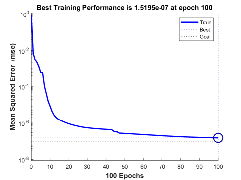
Figure 4: Mean Squared Error (MSE) of SFBC-NN for content popularity prediction.

(a) Comparisons of real trajectory and prediction trajectory.

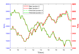
(b) Comparisons of real trajectory and predicted trajectory in X and Y axis

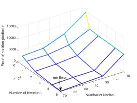
(c) Performance with the Number of Nodes and the Number of iterations.

Figure 5: The SFBC-NN prediction of users mobility (data from simulation).

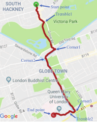
(a) Trajectory of a user in Google map.

(b) Comparisons of real trajectory and prediction trajectory.

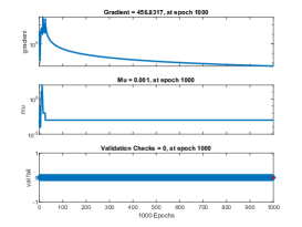
(c) Performance of SFBC-NN prediction (data measured from smartphone).

Figure 6: The SFBC-NN prediction of user’s mobility (data from smartphone).

V-A Simulation Results of Content Popularity Prediction

In this subsection, we utilize history data of content popularity to predict content popularity in the future. More precisely, content popularity in 5 time slots are provided as SFBC-NN input, while the output is content popularity in the next slot. As is shown in Fig. 4, MSE of the network decreases with epochs. It reached bottom after 50 epochs.

V-B Simulation Results of User Mobility Prediction

In order to analysis the mobility of users, firstly, we generate user’s positions through random work model. Fig. 5 evaluates the prediction accuracy of SFBC-NN based user position prediction. In Fig. 5(a), the red line shows user real trajectory, and blue points are predictions of user positions. As is shown is the Fig. 5(a) and 5(b), the predicted trajectory converges to the real trajectory, which clarifies that the trained weight parameters of SFBC neural network is capable of predict user position.

Fig. 5(c) shows the error of position prediction, where the error decreases with the number of nodes in SFBC-NN and that of iterations. This is because the increased number of nodes and iterations enhances the fitting capability of the network, thus strengthen the prediction accuracy. Due to the fact that a user position has only two dimensions, the simulation results show that SFBC-NN is powerful to deal with user mobility prediction.

Sociological researches have provided us various methods to collect people’s moving trajectory. However, it consumes a lot of resources (i.e., time, manpower, and money) to collect a large number of data. For this reason, we collect movements of one user, to validate the accuracy of our proposed prediction algorithm. In Fig. 6(a), we use measured data from smartphone to test the prediction accuracy of the SFBC-NN. The data is collected from daily life using GPS-tracker app on an Android smartphone. Fig. 6(a) shows the trajectory of user in Google Maps, and there are trembles and corners in the trajectory, which will effect prediction accuracy. The results indicated in Fig. 6(b) confirm the accuracy of SFBC neural network. This phenomenon is also confirmed by the insights in Remark 2. Fig. 6(c) shows performance of SFBC-NN based user mobility prediction. By indicating the gradual decreasement of gradient with training epoch number. Similarly mu also decreases to a stable state at approximately 20 epoches. And there are no fail observed.

(a) Q learning based caching.

(b) Optimal caching.

Figure 7: The MOS of users distributes in different positions of the area for different caching methods.

Figure 8: The MOS of different cache scheme vs. transmit power and the number of BSs and users.

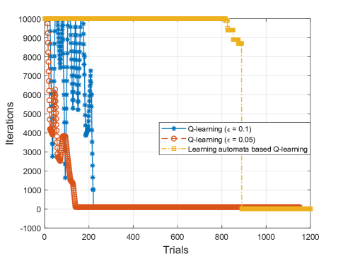
Figure 9: The reward curves of learning automata based Q-learning and conventional Q-learning over trials.

V-C Simulation Results of LAQL Based Cooperative Caching

In this subsection, we compare the proposed LAQL based cooperative caching with the above mentioned traditional caching schemes. Fig. 7 shows QoE distribution of users in this rectangle area, with different caching schemes, (i.e., Q-learning based caching and optimal caching). It can be observed that users near BSs have better QoE than those who are far from BSs. This is easy to understand because the distance between a user and a BS has important influence on MOS of the user, and also this can be further explored to analysis the deployment of BSs (i.e., deployment schemes and density of BSs).

Fig. 8 shows the overall MOS of users as a function of transmit power. We first adjust the learning rate $\alpha$ and discount factor $\gamma$ of traditional Q-learning algorithm, because $\alpha$ and $\gamma$ have significant influence of Q-learning. After several adjustment, we set $\alpha=0.75$ and $\gamma=0.6$. After that, we set the learning rate and discount factor of LAQL is the same as traditional Q-learning, aiming at reducing the interference of learning rate and discount factor between traditional Q-learning and LAQL. As can be seen from this figure, MOS increase with greater transmit power. We see that the performance of LAQL based cooperative caching is closer to optimal solution than traditional Q-learning, non-cooperative caching and random caching. This is because the action selection scheme of LAQL enables the agent to choose optimal action in each state, while action selection scheme in traditional Q-learning is based on a stochastic mechanism (i.e., $\epsilon$-greedy). Fig. 8 also shows that cooperative caching outperforms random caching and non-cooperative caching. The reason is that the cooperative caching takes user mobility and content popularity into consideration while random caching does not. Meanwhile, the cooperative caching is capable of better balance the caching resource in different BSs than non-cooperative caching.

Fig. 9 shows the iteration curves of LAQL and $\varepsilon$-greedy Q-learning. There are 10000 iterations in each trial. As can be seen from the figure, the curves of Q-learning fluctuate a lot, and with the increase of $\epsilon$, Q-learning takes more trials to converge. Also can be seen from Fig. 9, that the convergence of LAQL outperforms $\varepsilon$-greedy Q-learning eventually.

VI Conclusion

In this article, content cooperative caching scheme were studied along with user mobility and content popularity prediction for wireless communication system. In order to fulfill backhaul constraints, an optimization problem of users’ MOS maximization was formulated. 1) For user position and content popularity prediction, an SFBC-NN algorithm was proposed that utilized the powerful nonlinear fitting ability of SFBC-NN. The efficiency of the proposed scheme was validated by practical testing data set. 2) For content cooperative caching problem, a LAQL based cooperative caching algorithm was proposed, utilizing LA for optimal action selection in every state. The effectiveness of the proposed solution was illustrated by numerical experiments.

Appendix A: Proof of Lemma 1

The express of the objective function in (12) is (9). To prove that the optimization problem in (12) is NP-hard. We first consider the NP-hardness of the following problem.

Problem 1 ($N$-Disjoint Set Cover Problem).

Given a set $\mathcal{A}$ and a collection $\mathcal{B}$, the $N$-disjoint set cover problem is to determine whether $\mathcal{B}$ can be divided into $N$ disjoint set covers or not. More generally, consider a bipartite graph $\mathcal{G}=\left({\mathcal{A},\mathcal{B},\mathcal{E}}\right)$ with edges $\mathcal{E}$ between two disjoint vertex sets $\mathcal{A}$ and $\mathcal{B}$. Thus the $N$-disjoint set cover problem is whether there exist $N$ disjoint sets ${{\cal B}_{1}},{{\cal B}_{2}},\cdots{{\cal B}_{N}}\subset{\cal B}$ in which $\left|{{{\cal B}_{1}}}\right|+\left|{{{\cal B}_{2}}}\right|+\cdots+\left|{{{\cal B}_{N}}}\right|=\left|{\cal B}\right|$ and ${\cal A}=\mathop{U}\limits_{\textbf{B}\in{{\cal B}_{1}}}N\left(\textbf{B}\right)=\mathop{U}\limits_{\textbf{B}\in{{\cal B}_{2}}}N\left(\textbf{B}\right)=\cdots=\mathop{U}\limits_{\textbf{B}\in{{\cal B}_{N}}}N\left(\textbf{B}\right)$. The $N$-disjoint set cover problem can be denoted as $\textbf{{NDSC}}\left({{\cal A},{\cal B},{\cal E}}\right)$.

According to [43], the $\textbf{NDSC}\left({{\cal A},{\cal B},{\cal E}}\right)$ is proved to be NP-complete when $\left({N\geq 2}\right)$. Consider $\mathcal{A}$ to be the set of mobile users, $\mathcal{B}$ to be BSs with caching capacity, and $\mathcal{E}$ to be the edges representing connections between mobile users and BSs. The content popularity is $P=\left[{{p_{1}},{p_{2}},\cdots,{p_{F}}}\right]$ where ${p_{f}}<1$ for $\forall f\in\mathcal{F}$. Without loss of generality, we set the caching capacity of each BS is equals to 1, which means that each BS can cache only one content. According to (9), the maximization of the total MOS of users can only be gained by the BS caches all the contents that the user requested. In other words, each user has at least one neighboring BS caching content 1 and other neighboring BS caching contents 2 to $F$. Letting ${{{\cal B}_{1}}}$, ${{{\cal B}_{2}}}$, and ${{{\cal B}_{F}}}$ be the disjoint sets of BSs containing file 1 to file $F$, separately. We conclude that determining whether the objective function (12) is maximized is equivalent to determining the existence of and forming a $N$-disjoint set cover problem. From the analysis above, one can conclude that problem (12) is NP-hard.

Appendix B: Proof of Lemma 2

We shall prove Lemma 2 in two steps. Firstly, we show that we can convert the average reward value for an action to a reward probability, given that a higher average reward corresponds a higher reward probability. In other words, we need to map the value of Q value from ($-\infty$, $+\infty$) to ($0,1$). This conversion can be done by a modified arctangent-shape function, as shown in Fig. 10. Given that $Q(s,a)$ can converge to the optimal Q value, we can be certain that there exists a long term stationary reward behind each action of each state, and thus a stationary reward probability after conversion. Secondly, we need to show that the LA is $\epsilon$-optimal in the random and stationary environment, represented by the reward probability behind each action, but hidden before learning. The proof of $\epsilon$-optimal is not trivial and the detailed proof can be found in [40]. Here we just outline the main steps of the proof presently.

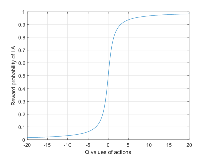
Figure 10: Mapping reward value to probability.

Now let’s suppose there are $r$ actions for state $s$. The real reward in probability for action $i$, after conversion from the long term average reward value of action $i$, is $d_{i}$. Correspondingly, the estimated reward probability by the LA for action $i$ at time $t$ is $\hat{d}(t)_{i}$, where $i\in\{1,\ldots,r\}$. Define $\mathbb{D}=[d_{1},\ldots,d_{r}]$ and $\hat{\mathbb{D}}(t)=[\hat{d}_{1}(t),\ldots,\hat{d}_{r}(t)]$. Let action probability vector be $\mathbb{P}(t)=[p_{1}(t),p_{2}(t),...,p_{r}(t)]$, which is used to determine the issue of which action is to be selected at $t$, where $\sum\limits_{j=1...r}{p_{j}(t)}=1$. Let $m$ be the index of the optimal action. To show the $\epsilon$-optimality of LA, we need to prove that given any $\epsilon>0$ and $\delta>0$, there exist an $N_{0}>0$ and a $t_{0}<\infty$ such that for all time $t\geq t_{0}$ and for any positive learning parameter $N>N_{0}$,

$$Pr\{p_{m}(t)>1-\epsilon\}>1-\delta.$$ (21)

This result has been proven in [40], and we illustrate here only the outline of the proof, just for a quick reference to the theorem that has been used to support the result. One is recommended to refer to the original paper for a thorough elaboration of the reasoning.

The $\epsilon$-optimality of the DPA was based on the submartingale property of the Action Probability sequence $\{p_{m}(t)_{t>t_{0}}\}$. Thus the submartingale convergence theory and the theory of Regular functions were invoked to prove that the DPA will converge to the optimal action in probability, i.e., $Pr\{p_{m}(\infty)=1\}\rightarrow 1$.

$\{p_{m}(t)_{t>t_{0}}\}$ being a submartingale was proven by the definition of submartingale. Firstly, $p_{m}(t)$ is a probability, hence $E[p_{m}(t)]\leq 1<\infty$ holds. Secondly, according to the learning mechanism of DPA, the expectation of $p_{m}(t)$ can be calculated explicitly as:

$$E[p_{m}(t+1)|\mathbb{P}(t)]$$

$$= \sum\limits_{j=1...r}{p_{j}(t)\left(d_{j}\left(q(t)(p_{m}(t)+c_{t}\Delta)+(1-q(t))(p_{m}(t)-\Delta)\right)+(1-d_{j})p_{m}(t)\right)}$$

$$= p_{m}(t)+\sum\limits_{j=1...r}{p_{j}(t)d_{j}\left(q(t)(c_{t}\Delta+\Delta)-\Delta\right)},$$

where $q(t)=Pr(\hat{d}_{m}(t)>\hat{d}_{i}(t))$, $\forall i\neq m$, is the accuracy probability of the reward estimates. By the definition of submartingale, one can see that if $\forall t>t_{0},~{}~{}~{}q(t)>\frac{\Delta}{c_{t}\Delta+\Delta}=\frac{1}{c_{t}+1}\geq\frac{1}{2}$ holds, then $E[p_{m}(t+1)|\mathbb{P}(t)]>p_{m}(t)$ becomes true, and $\{p_{m}(t)_{t>t_{0}}\}$ is thus a submartingale.

It has been proven in [40] that the accuracy probability of the reward estimates can be arbitrarily high. The proof itself involves quite a bit algebraic manipulations, and is thus complicated, but the rationale behind it is straight forward. It proved that after $t_{0}$, each action, with a very high probability, will be selected for a large number of times. Then, given that each action has been tried for a large number of times, the estimate of its reward will certainly become accurate enough to surpass the number $\frac{1}{2}$, which grantees $\{p_{m}(t)_{t>t_{0}}\}$ for being a submartingale.

Once the submartingale property is proven, by the submartingale convergence theory, $p_{m}(\infty)=0\text{~{}or~{}}1$ holds. To prove the DPA converges to the optional action, we need to shown that $p_{m}(\infty)=1$ will happen with arbitrarily large probability, rather than $p_{m}(\infty)=0$. This is then equivalent to proving the convergence probability below

$$\Gamma_{m}(\mathbb{P})=Pr\{\mathbb{P}(\infty)=\mathbb{e}_{m}|\mathbb{P}(0)=\mathbb{P}\}\rightarrow 1,$$ (22)

where $\mathbb{e}_{j}$ is the unit vector with the $j^{th}$ element being $1$. To prove Eq. (22), we now need to clarify the following definitions [44]:

$\Phi(\mathbb{P})$: a function of $\mathbb{P}$.

$U$: an operator such that $U\Phi(\mathbb{P})=E[\Phi(\mathbb{P}(n+1))|\mathbb{P}(n)=\mathbb{P}],$
           applying $U$ for $n$ times: $U^{n}\Phi(\mathbb{P})=E[\Phi(\mathbb{P}(n))|\mathbb{P}(0)=\mathbb{P}].$

The function $\Phi(\mathbb{P})$ is:

• Superregular: If $U\Phi(\mathbb{P})\leq\Phi(\mathbb{P})$. Then applying $U$ repeatedly yields:

  $$\Phi(\mathbb{P})\geq U\Phi(\mathbb{P})\geq U^{2}\Phi(\mathbb{P})\geq...\geq U^{\infty}\Phi(\mathbb{P}).$$ (23)

• Subregular: If $U\Phi(\mathbb{P})\geq\Phi(\mathbb{P})$. In this case, if we apply $U$ repeatedly, we have

  $$\Phi(\mathbb{P})\leq U\Phi(\mathbb{P})\leq U^{2}\Phi(\mathbb{P})\leq...\leq U^{\infty}\Phi(\mathbb{P}).$$ (24)

• Regular: If $U\Phi(\mathbb{P})=\Phi(\mathbb{P})$. In such a case, it follows that:

  $$\Phi(\mathbb{P})=U\Phi(\mathbb{P})=U^{2}\Phi(\mathbb{P})=...=U^{\infty}\Phi(\mathbb{P}).$$ (25)

If we suppose $\Phi(\mathbb{P})$ satisfies the boundary conditions $\Phi(\mathbb{e}_{m})=1\text{~{}and~{}}\Phi(\mathbb{e}_{j})=0,(\forall j\neq m)$, then, one can calculate $U^{\infty}\Phi(\mathbb{P})$ and obtain very interesting results as follows:

$$U^{\infty}\Phi(\mathbb{P}) =E[\Phi(\mathbb{P}(\infty))|\mathbb{P}(0)=\mathbb{P}]$$

$$=\sum_{j=1}^{r}{\Phi(\mathbb{e}_{j})Pr\{\mathbb{P}(\infty)=\mathbb{e}_{j}|\mathbb{P}(0)=\mathbb{P}\}},~{}~{}\textit{~{}the ~{}definition~{} of~{} Expectation}$$

$$={\Phi(\mathbb{e}_{m})Pr\{\mathbb{P}(\infty)=\mathbb{e}_{m}|\mathbb{P}(0)=\mathbb{P}\}},~{}~{}\textit{~{}the ~{}boundry~{} condition $\Phi(\mathbb{e}_{j})=0$, $\forall~{}j\neq m$}$$

$$=Pr\{\mathbb{P}(\infty)=\mathbb{e}_{m}|\mathbb{P}(0)=\mathbb{P}\},~{}~{}\textit{~{}the ~{}boundry~{} condition $\Phi(\mathbb{e}_{m})=1$}$$

$$=\Gamma_{m}(\mathbb{P}).$$ (26)

This equation tells that the convergence probability can be studied by applying $U$ an infinite number of times to the function $\Phi(\mathbb{P})$. What’s more, if $\Phi(\mathbb{P})$ is a Regular function, the sequence of operations will lead to a function that equals the function $\Phi(\mathbb{P})$ itself, whereas if $\Phi(\mathbb{P})$ is a subregular/superregular function, the sequence of operations can be bounded from below/above by $\Phi(\mathbb{P})$.

What the authors have done in [40], is to find a subregular function of $\mathbb{P}$ that meets the boundary conditions, to bound the convergence probability of $\Gamma_{m}(\mathbb{P})$ from below. Then they proved the subregular function itself converges to unity, thus implies that the convergence probability, which is greater than or equal to the subregular function of $\mathbb{P}$, will converge to unity as well.

References

- [1] Z. Yang, Y. Liu, and Y. Chen, “Q-learning for content placement in wireless cooperative caching,” in Proc. IEEE Global Commun. Conf. (GLOBECOM), Abu Dhabi, UAE, Dec. 2018.
- [2] J. Montalban, P. Scopelliti, and et al., “Multimedia multicast services in 5G networks: Subgrouping and non-orthogonal multiple access techniques,” IEEE Commun. Mag., vol. 56, no. 3, pp. 91–95, Mar. 2018.
- [3] Cisco, Cisco visual networking index: Global mobile data traffic forecast update, 2016-2021. White paper, Feb. 2017.
- [4] Z. Qin, J. Fan, Y. Liu, Y. Gao, and G. Y. Li, “Sparse representation for wireless communications: A compressive sensing approach,” IEEE Signal Process. Mag., vol. 35, no. 3, pp. 40–58, May 2018.
- [5] Z. Qin, Y. Gao, M. D. Plumbley, and C. G. Parini, “Wideband spectrum sensing on real-time signals at sub-Nyquist sampling rates in single and cooperative multiple nodes,” IEEE Trans. Signal Process., vol. 64, no. 12, pp. 3106–3117, Jun. 2016.
- [6] Y. Liu, Z. Qin, M. Elkashlan, Z. Ding, A. Nallanathan, and L. Hanzo, “Nonorthogonal multiple access for 5G and beyond,” Proceedings of the IEEE, vol. 105, no. 12, pp. 2347–2381, Dec. 2017.
- [7] S. Tombaz, P. Monti, and et al., “Is backhaul becoming a bottleneck for green wireless access networks?” in IEEE Proc. of International Commun. Conf. (ICC), Jun. 2014.
- [8] A. Ioannou and S. Weber, “A survey of caching policies and forwarding mechanisms in information-centric networking,” IEEE Commun. Surv. Tut., vol. 18, no. 4, pp. 2847–2886, Fourthquarter 2016.
- [9] D. Liu, B. Chen, C. Yang, and A. F. Molisch, “Caching at the wireless edge: design aspects, challenges, and future directions,” IEEE Commun. Mag., vol. 54, no. 9, pp. 22–28, Sep. 2016.
- [10] J. Liao, K. K. Wong, Y. Zhang, Z. Zheng, and K. Yang, “Coding, multicast, and cooperation for cache-enabled heterogeneous small cell networks,” IEEE Trans. Wireless Commun., vol. 16, no. 10, pp. 6838–6853, Oct. 2017.
- [11] S. Zhang, P. He, K. Suto, P. Yang, L. Zhao, and X. S. Shen, “Cooperative edge caching in user-centric clustered mobile networks,” IEEE Trans. Mob. Comput., vol. 8, no. 99, pp. 1791–1805, Aug. 2018.
- [12] Y. Wang, X. Tao, X. Zhang, and Y. Gu, “Cooperative caching placement in cache-enabled D2D underlaid cellular network,” IEEE Commun. Lett., vol. 21, no. 5, pp. 1151–1154, May 2017.
- [13] Y. Liu, Z. Qin, M. Elkashlan, A. Nallanathan, and J. A. McCann, “Non-orthogonal multiple access in large-scale heterogeneous networks,” IEEE J. Sel. Areas Commun., vol. 35, no. 12, pp. 2667–2680, Dec. 2017.
- [14] W. Jiang, G. Feng, and S. Qin, “Optimal cooperative content caching and delivery policy for heterogeneous cellular networks,” IEEE Trans. Mob. Comput., vol. 16, no. 5, pp. 1382–1393, May 2017.
- [15] F. Wang, J. Xu, X. Wang, and S. Cui, “Joint offloading and computing optimization in wireless powered mobile-edge computing systems,” IEEE Trans. Commun. Technol., vol. 17, no. 3, pp. 1784–1797, Mar. 2018.
- [16] Y. Liu, Z. Qin, M. Elkashlan, Y. Gao, and L. Hanzo, “Enhancing the physical layer security of non-orthogonal multiple access in large-scale networks,” IEEE Trans. Wireless Commun., vol. 16, no. 3, pp. 1656–1672, Mar. 2017.
- [17] Z. Qin, H. Ye, and G. L. and et al., “Deep learning in physical layer communications,” ArXiv, 2018. [Online]. Available: https://arxiv.org/abs/1807.11713
- [18] D. Silver, A. Huang, and et al., “Mastering the game of go with deep neural networks and tree search,” Nature, vol. 529, no. 7587, pp. 484–489, Jan. 2016.
- [19] V. Mnih, K. Kavukcuoglu, D. Silver, and et al., “Playing atari with deep reinforcement learning,” ArXiv, 2013. [Online]. Available: https://arxiv.org/abs/1312.5602
- [20] V. Mnih, K. Kavukcuoglu, and et al., “Human-level control through deep reinforcement learning,” Nature, vol. 518, no. 7540, pp. 529–533, Feb. 2015.
- [21] O. A. S. Muller and et al., “Context-aware proactive content caching with service differentiation in wireless networks,” IEEE Trans. Wireless Commun., vol. 16, no. 2, pp. 1024–1036, Feb. 2017.
- [22] Q. Li, W. Shi, X. Ge, and Z. Niu, “Cooperative edge caching in software-defined hyper-cellular networks,” IEEE J. Sel. Areas Commun., vol. 35, no. 11, pp. 2596–2605, Nov. 2017.
- [23] R. Ghanavi, E. Kalantari, M. Sabbaghian, H. Yanikomeroglu, and A. Yongacoglu, “Efficient 3D aerial base station placement considering users mobility by reinforcement learning,” ArXiv, 2018. [Online]. Available: https://arxiv.org/abs/1801.07472
- [24] M. Chen, W. Saad, C. Yin, and M. Debbah, “Echo state networks for proactive caching in cloud-based radio access networks with mobile users,” IEEE Trans. Wireless Commun., vol. 16, no. 6, pp. 3520–3535, Jun. 2017.
- [25] M. Chen, W. Saad, and C. Yin, “Virtual Reality over Wireless Networks: Quality-of-Service Model and Learning-Based Resource Management,” ArXiv, 2017. [Online]. Available: https://arxiv.org/abs/1703.04209v2
- [26] S. O. Somuyiwa, A. György, and D. Gündüz, “A reinforcement-learning approach to proactive caching in wireless networks,” ArXiv, 2017. [Online]. Available: http://arxiv.org/abs/1712.07084
- [27] S. Wang, H. Liu, P. H. Gomes, and B. Krishnamachari, “Deep reinforcement learning for dynamic multichannel access in wireless networks,” IEEE Cog. Commun. Netw., pp. 1–1, 2018.
- [28] E. B. G. Paschos and et al., “Wireless caching: technical misconceptions and business barriers,” IEEE Commun. Mag., vol. 54, no. 8, pp. 16–22, August 2016.
- [29] Y. Liu, Z. Ding, M. Elkashlan, and H. V. Poor, “Cooperative non-orthogonal multiple access with simultaneous wireless information and power transfer,” IEEE J. Sel. Areas Commun., vol. 34, no. 4, pp. 938–953, Apr. 2016.
- [30] A. Sadeghi, F. Sheikholeslami, and G. B. Giannakis, “Optimal and scalable caching for 5G using reinforcement learning of space-time popularities,” IEEE J. Sel. Areas Commun., vol. 12, no. 1, pp. 180–190, Feb. 2018.
- [31] P. Document, “Definition of quality of experience (QoE),” document COM 12-LS 62-E, ITU-T, January 2007.
- [32] Y. Wang, W. Zhou, and P. Zhang, QoE Management in Wireless Networks, 3rd ed. Springer International Publishing, 2017.
- [33] M. Rugelj, U. Sedlar, M. Volk, and et al., “Novel cross-layer QoE-aware radio resource allocation algorithms in multiuser OFDMA systems,” IEEE Trans. Commun., vol. 62, no. 9, pp. 3196–3208, Sep. 2014.
- [34] P. Ameigeiras, J. J. Ramos-Munoz, J. Navarro-Ortiz, P. Mogensen, and J. M. Lopez-Soler, “QoE oriented cross-layer design of a resource allocation algorithm in beyond 3G systems,” Computer Communications, vol. 33, no. 5, pp. 571–582, 2010.
- [35] K. Hornik, “Approximation capabilities of multilayer feedforward networks,” Neural Networks, vol. 4, no. 2, pp. 251 – 257, 1991.
- [36] Y. Bengio, P. Lamblin, D. Popovici, and H. Larochelle, “Greedy layer-wise training of deep networks,” in Advances in neural information processing systems, 2007, pp. 153–160.
- [37] C. Szegedy, W. Zaremba, I. Sutskever, J. Bruna, D. Erhan, I. Goodfellow, and R. Fergus, “Intriguing properties of neural networks,” ArXiv, 2013. [Online]. Available: http://arxiv.org/abs/1312.6199
- [38] K. Shanmugam, N. Golrezaei, A. G. Dimakis, A. F. Molisch, and G. Caire, “Femtocaching: Wireless content delivery through distributed caching helpers,” IEEE Trans. Inf. Theory, vol. 59, no. 12, pp. 8402–8413, Dec 2013.
- [39] R. S. Sutton and A. G. Barto, Reinforcement Learning: An Introduction. Cambridge, MA, USA: MIT Press, 2016.
- [40] X. Zhang, B. J. Oommen, O.-C. Granmo, and L. Jiao, “A formal proof of the optimality of discretized pursuit algorithms,” Applied Intelligence, vol. 44, no. 2, pp. 282–294, Mar 2016.
- [41] X. Zhang, L. Jiao, J. B. Oommen, and O.-C. Granmo, “A conclusive analysis of the finite-time behavior of the discretized pursuit learning automaton,” IEEE Trans. neural net. learning sys., Feb. 2019.
- [42] J. Karedal, A. J. Johansson, F. Tufvesson, and A. F. Molisch, “A measurement-based fading model for wireless personal area networks,” IEEE Trans. Wireless Commun., vol. 7, no. 11, pp. 4575–4585, Nov. 2008.
- [43] C. Mihaela and D. Ding-Zhu, “Improving wireless sensor network lifetime through power aware organization,” Wireless Networks, vol. 11, no. 3, pp. 333–340, May 2005.
- [44] K. S. Narendra and M. A. Thathachar, Learning automata: an introduction. Courier Corporation, 2012.