Mobility edge of two interacting particles in three-dimensional random potentials

Abstract

We investigate Anderson transitions for a system of two particles moving in a three-dimensional disordered lattice and subject to on-site (Hubbard) interactions of strength $U$. The two-body problem is exactly mapped into an effective single-particle equation for the center of mass motion, whose localization properties are studied numerically. We show that, for zero total energy of the pair, the transition occurs in a regime where all single-particle states are localized. In particular the critical disorder strength exhibits a non-monotonic behavior as a function of $|U|$, increasing sharply for weak interactions and converging to a finite value in the strong coupling limit. Within our numerical accuracy, short-range interactions do not affect the universality class of the transition.

I Introduction and motivations

Wave diffusion in disordered media can be completely inhibited Anderson (1958) due to interference effects between the multiple scatterings from the randomly distributed impurities. This phenomenon, known as Anderson localization, has been observed for several kinds of wave-like systems, including light waves in diffusive media Wiersma et al. (1997); Störzer et al. (2006) or photonic crystals Schwartz et al. (2007); Lahini et al. (2008), ultrasound Hu et al. (2008), microwaves Chabanov et al. (2000) and atomic matter waves Billy et al. (2008); Roati et al. (2008).

In quantum systems, this effect appears through the spatial localization of the wave-functions. In the absence of magnetic fields and of spin-orbit couplings, all states are exponentially localized in one and in two dimensions, whereas in three dimensions there exists a critical value $E_{c}$ of the particle energy, called mobility edge, separating localized from extended states. At this point the system undergoes a metal-insulator transition Evers and Mirlin (2008). Mobility edges have been reported Kondov et al. (2011); Jendrzejewski et al. (2012); Semeghini et al. (2015) in experiments with non-interacting ultracold atoms in three-dimensional (3D) speckle potentials, and their measured values have been compared against precise numerical estimates Delande and Orso (2014); Fratini and Pilati (2015a); Pasek et al. (2015); Fratini and Pilati (2015b); Pasek et al. (2017). Interestingly, Anderson transitions have also been observed Chabé et al. (2008) in momentum space, using cold atoms implementations of the quasi-periodic quantum kicked rotor, allowing for the first experimental test of universality Lopez et al. (2012). For a correlated disorder, mobility edges occur even in lower dimensions, as recently observed Lüschen et al. (2018) for atoms in one-dimensional quasi-periodic optical lattices, in agreement with earlier theoretical predictions Boers et al. (2007); Li et al. (2017).

While single-particle Anderson localization is relatively well understood, its generalization to interacting systems, called many-body localization, is more recent Basko et al. (2006) and is currently the object of intense theoretical and experimental activities Nandkishore and Huse (2015); Abanin et al. (2019); Parameswaran and Vasseur (2018). Perhaps surprisingly, even the problem of two interacting particles in a random potential is still open. In a seminal work Shepelyansky (1994), Shepelyansky showed that, in the presence of a weak (attractive or repulsive) interaction, a pair can propagate over a distance much larger than the single-particle localization length. It was later argued Borgonovi and Shepelyansky (1995); Imry (1995) that all two-particle states remain localized in one and two dimensions (although with a possibly large localization length), whereas in three dimensions an Anderson transition to a diffusive phase could occur even when all single-particle states are localized. While several numerical studies Weinmann et al. (1995); von Oppen et al. (1996); Frahm (1999); Roemer et al. (2001); Dias and Lyra (2014); Lee et al. (2014); Krimer and Flach (2015); Frahm (2016) have confirmed the claim for one-dimensional systems, the situation is much less clear in higher dimensions, where the computational cost limits the system sizes that can be explored. In particular an Anderson transition was predicted Ortuño and Cuevas (1999); Roemer et al. (1999) to occur in two dimensions (see also Chattaraj (2018) for a recent study of the two-particle dynamics in a similar model).

In this work we investigate Anderson transitions in a system of two particles moving in a 3D disordered lattice and coupled by on-site interactions. The particles can be either bosons or fermions with different spins in the singlet state. Based on large-scale numerical calculations of the transmission amplitude, we compute the precise phase boundary between localized and extended states in the interaction-disorder plane, for a pair with zero total energy (well above the ground state). Importantly, we find that the two-particle Anderson transition is still described by the orthogonal universality class.

In Sec. II we map exactly the two-particle Hamiltonian into an effective single-particle model, Eq.(3), and compute the associated matrix $K$. In Sec. III we explain how to extract the reduced localization length of a pair with zero total energy from transmission amplitude calculations performed in short bars. We then identify the critical point of the Anderson transition via an accurate finite-size scaling analysis. In Sec. IV we present the phase diagram for Anderson localization of the pair in the interaction-disorder plane.

II Effective single-particle model

The two-body Hamiltonian can be written as $\hat{H}=\hat{H}_{0}+\hat{U}$, where $\hat{U}=U\sum_{\mathbf{m}}|{\mathbf{m}},{\mathbf{m}}\rangle\langle{\mathbf{m}},{\mathbf{m}}|$ refers to the on-site (Hubbard) interaction of strength $U$ and $\hat{H}_{0}$ is the non interacting part. The latter can be written as $\hat{H}_{0}=\hat{H}^{\textrm{sp}}\otimes\hat{\mathds{1}}+\hat{\mathds{1}}\otimes\hat{H}^{\textrm{sp}}$, where

$$\hat{H}^{\textrm{sp}}=-J\sum_{\mathbf{n},i}|\mathbf{n}+\mathbf{e}_{i}\rangle\langle\mathbf{n}|+\sum_{\mathbf{n}}V_{\mathbf{n}}|\mathbf{n}\rangle\langle\mathbf{n}|$$ (1)

is the single-particle Anderson model. Here $J$ is the tunneling rate between neighboring sites, $\mathbf{e}_{i}$ are the unit vectors along the three orthogonal axes and $V_{\mathbf{n}}$ is the value of the random potential at site $\mathbf{n}$. In the following we fix the energy scale by setting $J=1$ and assume that the random potential is uniformly distributed in the interval $[-W/2,W/2]$. Then all single-particle states are localized for $W>W_{c}^{sp}=16.54\pm 0.01$ McKinnon and Kramer (1983); Slevin and Ohtsuki (2014).

The Schrödinger equation for the pair can be written as $(E-\hat{H}_{0})|\psi\rangle=\hat{U}|\psi\rangle$, $E$ being the total energy. Applying the Green’s function operator $\hat{G}(E)=(E\hat{I}-\hat{H}_{0})^{-1}$ to both sides of this equation, we find

$$|\psi\rangle=\sum_{\mathbf{m}}U\hat{G}(E)|{\mathbf{m}},{\mathbf{m}}\rangle\langle{\mathbf{m}},{\mathbf{m}}|\psi\rangle,$$ (2)

showing that the wave-function can be completely reconstructed from the diagonal amplitudes $f_{\mathbf{m}}=\langle{\mathbf{m}},{\mathbf{m}}|\psi\rangle$. By projecting Eq.(2) over the state $|{\mathbf{n}},{\mathbf{n}}\rangle$, we see that such terms obey a close equation Dufour and Orso (2012); Orso et al. (2005):

$$\sum_{\mathbf{m}}K_{\mathbf{n}\mathbf{m}}f_{\mathbf{m}}=\frac{1}{U}f_{\mathbf{n}},$$ (3)

where $K_{\mathbf{n}\mathbf{m}}=\langle{\mathbf{n}},{\mathbf{n}}|\hat{G}(E)|{\mathbf{m}},{\mathbf{m}}\rangle$. Hence, for a given energy $E$ of the pair, Eq.(3) can be interpreted as an effective single-particle Schrodinger problem with eigen-energy $\lambda=1/U$. The main purpose of this work is to compute the associated mobility edge $U_{c}(W)$, for $E=0$.

We start by considering a 3D grid with transverse size $M$ and longitudinal size $L$. Differently from the 3D Anderson model, the matrix $K$ of the effective Hamiltonian is dense and its elements have to be calculated numerically by expressing them in terms of the eigenbasis of the single-particle model, $\hat{H}^{\textrm{sp}}|\phi_{r}\rangle=\varepsilon_{r}|\phi_{r}\rangle$:

$$K_{\mathbf{n}\mathbf{m}}=\sum_{r=1}^{N}\phi_{\mathbf{n}r}\phi_{\mathbf{m}r}^{*}\langle\mathbf{n}|G^{\textrm{sp}}\mathbf{(}E-\varepsilon_{r})|{\mathbf{m}}\rangle,$$ (4)

where $G^{\textrm{sp}}(\varepsilon)=(\varepsilon I-H^{\textrm{sp}})^{-1}$ is the associated matrix resolvent, $I$ is the identity matrix and $\phi_{\mathbf{n}r}=\langle\mathbf{n}|\phi_{r}\rangle$. The eigenbasis is calculated by imposing open boundary conditions along the bar and periodic boundary conditions in the transverse directions. We see from Eq.(4) that the computation of the matrix $K$ requires $N$ inversions of $N\times N$ matrices, $N=M^{2}L$ being the total number of sites. The matrix inversion is efficiently performed via recursive techniques Jain et al. (2007), exploiting the block tridiagonal structure of the Hamiltonian (1). This allows to reduce the number of elementary operations from $N^{3}$, holding for a general matrix, to $M^{6}L^{2}$. Hence the total cost for the evaluation of $K$ scales as $M^{8}L^{3}$, which broadly exceeds the cost $M^{6}L$ of transfer matrix simulations for the same grid McKinnon and Kramer (1983). This drastically limits the system sizes that we can explore. In our numerics we keep the length of the bar fixed to $L=150$ and vary the transverse size $M$ between $8$ and $17$.

III NUMERICAL DETERMINATION OF THE CRITICAL POINT

The logarithm of the transmission amplitude of the pair, evaluated at a position $n_{z}$ along the bar, is given by McKinnon and Kramer (1983):

$$F(n_{z})=\ln\sum_{\mathbf{m}_{\perp},\mathbf{n}_{\perp}}|\langle\mathbf{m}_{\perp},1|G^{\textrm{p}}(\lambda)|\mathbf{n}_{\perp},n_{z}\rangle|^{2},$$ (5)

where $G^{\textrm{p}}(\lambda)=(\lambda I-K)^{-1}$ is the matrix resolvent of the effective model, $\mathbf{m}_{\perp}=(m_{x},m_{y})$ and $\mathbf{n}_{\perp}=(n_{x},n_{y})$. In the limit $L\gg M$ the function (5) approaches a straight line, whose slope $p$ determines the Lyapunov exponent $\gamma$ according to $\gamma=-p/2$. The reduced localization length, needed for the finite-size scaling analysis, is defined as $\Lambda_{M}=1/(\bar{\gamma}M)$, where $\bar{\gamma}$ is the disorder-averaged Lyapunov exponent.

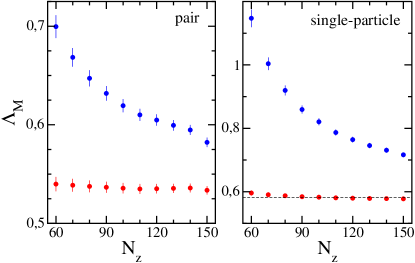
Figure 1: Left panel: convergence study of the reduced localization length $\Lambda_{M}=1/(\bar{\gamma}M)$ of the pair as a function of the position $N_{z}$ along the bar. Here $\bar{\gamma}$ denotes the Lyapunov exponent, averaged over $N_{tr}=701$ different disorder realizations, while the length and the transverse size of the bar are $L=150$ and $M=12$, respectively. The upper curve is obtained by calculating the Lyapunov exponent, for each disorder realization, via $\gamma=-F(N_{z})/(2N_{z})$, where $F$ is defined in Eq.(5). The lower curve is instead obtained by fitting the data $(n_{z},F(n_{z}))$ with $n_{z}=10,20,...,N_{z}$ by a straight line, $f_{fit}(n_{z})=pn_{z}+q$, and setting $\gamma=-p/2$. Only the fitting method yields converged results. The total energy of the pair is $E=0$, while the Hamiltonian parameters are $W=23.5$ and $U=2$. Right panel: same analysis but for the single-particle Anderson model, Eq.(1), for $\varepsilon=0$ (middle of the band) and $W=16.5$. The values of $L,M$ and $N_{tr}$ are the same as in the left panel. The dashed line corresponds to the estimate $\Lambda_{M}=0.5814\pm 0.0004$ obtained from transfer-matrix calculations performed on a bar of length $L=10^{5}$ after averaging over $240$ disorder realizations.

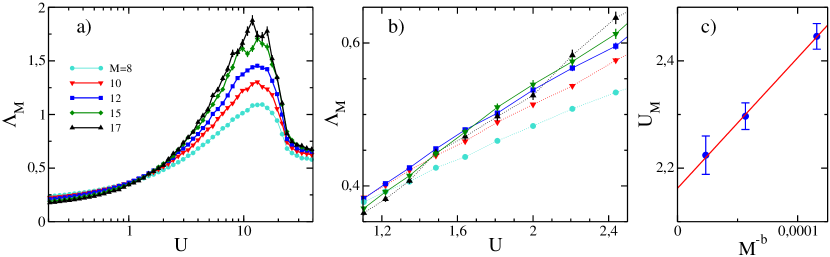
Figure 2: a) Reduced localization length as a function of the interaction strength for increasing values of the transverse size $M=8,10,12,15,17$ of the bar, calculated using the fitting method. The energy of the pair is $E=0$ and the disorder strength is $W=23.5$, implying that all single-particle states are localized. The transition takes place at the point where all data curves with sufficiently large $M$ cross. b) Zoom of the region containing the crossing points for the largest system sizes. To improve visibility, data points for $M=8,10,17$ are connected by dotted lines. c) Numerical determination of the critical point: the value $U_{M}$, defined by $\Lambda_{M}(U=U_{M})=\Lambda_{c}$, is plotted as a function of $M^{-b}$ for $M=10,12,15$. For the orthogonal class $\Lambda_{c}=0.576$ and $b=3.94\pm 0.6$. The straight line represents a fit to the data, whose intercept yields the critical value $U_{c}=2.16\pm 0.04$.

In order to extrapolate it to $L\rightarrow+\infty$ from our short bar, we proceed as follows. For each disorder realization, we evaluate $F(n_{z})$ at regular intervals along the bar and extract the slope by a linear fit, $f_{fit}(n_{z})=pn_{z}+q$. For a given position $N_{z}$ along the bar, we calculate the slope by fitting only data points with $n_{z}\leq N_{z}$. The results calculated for $M=12,W=23.5$ and $U=2$ are displayed in the left panel of Fig.1 (bottom data curve). We see that the curve is rather flat as $N_{z}$ approaches $L$, suggesting that our fitting procedure is correct (see Supplemental Material myn ). For comparison, in Fig.1 we also show (upper curve) the unconverged results obtained by using $p=F(N_{z})/N_{z}$ (upper curve).

The right panel of Fig.1 presents the same analysis for the single-particle Hamiltonian (1) at zero energy, $\varepsilon=0$, and $W=16.5$. This is done by replacing $G^{\textrm{p}}$ with $G^{\textrm{sp}}$ in Eq.(5), keeping unchanged the size of the bar as well as the number of disorder realizations. The results based on the fitting method agree fairly well with the very accurate estimate obtained from transfer-matrix calculations (dashed line).

The critical point of the metal-insulator transition can be identified by studying the behavior of $\Lambda_{M}$ as a function of the interaction strength $U$ and for increasing values of the transverse size $M$. In the metallic phase, $\Lambda_{M}$ increases with $M$, while in the insulating regime $\Lambda_{M}$ decreases for $M$ large enough. Exactly at the critical point $\Lambda_{M}$ becomes scale-invariant, that is $\lim_{M\rightarrow+\infty}\Lambda_{M}=\Lambda_{c}$, where $\Lambda_{c}$ is a constant of order unity, which only depends on the universality class of the model and on the specific choice of boundary conditions. For example the Anderson model (1) belongs to the orthogonal universality class, where $\Lambda_{c,orth}=0.576$ assuming periodic boundary conditions in the transverse directions.

In Fig.2 (panel a) we plot our numerical results for the reduced localization length as a function of the interaction strength for increasing values of $M$ assuming $W=23.5$, so that all single-particle states are localized. Since $E=0$, the value of $\Lambda_{M}$ is independent of the sign of $U$, so hereafter we assume $U>0$. We see that interactions favor the delocalization of the pair and lead to an Anderson transition around $U=2$.

Identifying the precise position of the critical point is not straightforward, because the crossing point drifts towards stronger interactions and upwards as $M$ increases, due to finite size effects. Simulating systems with even larger values of $M$ is computationally prohibitive: the data for $M=17$, obtained by averaging $N_{tr}=470$ disorder realizations, required already 700000 hours of computational time on a state-of-the-art supercomputer, and the curve is not smooth.

As shown in the inset of Fig.(2) (panel b), the height of the crossing point for the largest system sizes (couples $M=12,17$ and $M=15,17$) becomes closer and closer to $\Lambda_{c,orth}$, suggesting that also the effective model for the pair belongs to the orthogonal universality class. In this case, no significant further drift is expected. To verify this hypothesis, we need to compute the critical exponent $\nu$ related to the divergence of the localization length at the critical point, $\xi\sim|U-U_{c}|^{-\nu}$, and compare it with the numerical value $\nu_{orth}=1.573$ known Slevin and Ohtsuki (2014) for the orthogonal class.

According to the one parameter scaling theory of localization and for large enough $M$, the reduced localization length can be written in terms of a scaling function $f$ as

$$\Lambda_{M}=f(u(\omega)M^{1/\nu}),$$ (6)

where $u$ is a function of the variable $\omega=(U-U_{c})/U_{c}$, measuring the distance from the critical point. Close to it, we can expand the scaling functions $u$ and $f$ in Eq.(6) in Taylor series up to orders $m$ and $n$, respectively, as $u(\omega)=\sum_{j=0}^{m}b_{j}\omega^{j}$ and $f(x)=\sum_{j=0}^{n}a_{j}x^{j}$. Following Slevin and Ohtsuki (2014), we set $b_{1}$=0, $a_{1}=0$ and $a_{0}=\Lambda_{c}$. The coefficients $a_{j}$ and $b_{j}$, as well as $U_{c}$ and $\nu$, are then obtained via a multilinear fit. We extract the critical exponent by fitting the (smoothest) data for $M=12$ and $M=15$ in the inset of Fig.2 with the ansatz (6). The latter should in principle include also irrelevant variables, describing the drift of the crossing point. However, unlike $U_{c}$ and $\Lambda_{c}$, the value of the critical exponent is much less sensitive to these variables. For $n=m=2$ we obtain $\nu=1.64\pm 0.13$, in full agreement with the universal value. All other crossings yield consistent results for $\nu$.

Having found that on-site interactions do not change the universality class of the transition, we can use this information to estimate $U_{c}$. Let $U_{M}$ be the value of the interaction strength at which $\Lambda_{M}(U=U_{M})=\Lambda_{c,orth}$. For sufficiently large $M$, one can show Campostrini et al. (2001) that $U_{M}=U_{c}+aM^{-b}$, where $a$ is a numerical constant and $b=1/\nu_{orth}+y_{orth}$. Here $y_{orth}$ is the leading irrelevant variable, whose value is also universal and given by $y_{orth}=3.3\pm 0.6$ Slevin and Ohtsuki (2014). In Fig.(2) (panel c) we show that the values of $U_{M}$ extracted from our data curves for $M=10,12,15$ do vary linearly as a function of $M^{-b}$. A linear fit to the data then yields $U_{c}=2.16\pm 0.04$.

IV Phase diagram

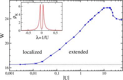
Figure 3: Main panel: phase boundary between localized and extended states in the $(U,W)$ plane, computed for a pair with zero total energy, $E=0$. The dashed horizontal line corresponds to the noninteracting limit, $W=W_{c}^{sp}=16.54$. The diagram holds for both attractive and repulsive interactions. Inset: disorder-averaged density of states $\rho_{K}$ of the effective Hamiltonian of the pair calculated for $W=23.5$ using a cubic grid of sizes $L=M=20$ with periodic boundary conditions.

Next, we map out the phase boundary between localized and extended states of the pair in the $(U,W)$ plane. For each value of the disorder strength, we calculate the reduced localization length as a function of $U$ for $M=10,12,15$ and extrapolate the critical point from the scaling behavior of the $U_{M}$ values. To save computer resources, we have limited the number of disorder realizations resulting in larger error bars for $U_{c}$. Moreover, for $W\leq 21$, we have calculated the intercept by discarding also the data for $M=10$, as the relative deviation $(U_{M}-U_{c})/U_{c}$ increases as $W$ decreases.

The obtained results are displayed in Fig.3. We see that the Anderson transition for a pair with zero total energy occurs in a region, where all single-particle states are localized (see also Supplemental Material myn ). For $23.7\leq W\leq 25.9$ the system possesses two distinct critical points, resulting in a nonmonotonic behavior of the phase boundary. This is best explained by calculating the disorder-averaged density of states of the effective model, $\rho_{K}(\lambda)=\overline{\sum_{r}\delta(\lambda-\lambda_{r})/N}$, $\lambda_{r}$ being the eigenvalues of the kernel $K$. The result for $W=23.5$ is displayed in the inset of Fig.3. We see that $\rho_{K}$ is strongly peaked at finite values of $\lambda$ and exhibits vanishing (power-law) tails. This can be understood starting from the strongly disordered limit, $W\gg 1$. Since hopping terms can be neglected, the kernel $K$ becomes diagonal, $K_{\mathbf{n}\mathbf{m}}=\delta_{\mathbf{n}\mathbf{m}}/(E-2V_{\mathbf{n}})$, implying that

$$\rho_{K}(\lambda)=\frac{1}{2W\lambda^{2}}\Theta\left(W-\left|E-\frac{1}{\lambda}\right|\right),$$ (7)

where $\Theta$ is the unit step function. In particular for $E=0$ the density of states vanishes for $|\lambda|<1/W$. Indeed, in order to interact, the two particles must lie on the same site $\mathbf{n}$, so the total energy is given by $E=U+2V_{\mathbf{n}}=0$, implying $|U|=2|V_{\mathbf{n}}|\leq W$. Reducing the disorder strength allows for tunneling between neighboring sites and leads to a finite value of $\rho_{K}(0)$, as shown in the inset of Fig.3. From the above discussion, one expects that weakly interacting states are the first to be localized by disorder, whereas states with $|U|\sim W$ are the most robust against localization, in agreement with the phase diagram of Fig.3.

It is worth mentioning that a nonmonotonic behavior of the critical disorder strength versus $U$ was also obtained for the ground state of the Anderson-Hubbard model at finite fillings in earlier theoretical studies Byczuk et al. (2005) Henseler et al. (2008) based, respectively, on the dynamical mean field theory and on the self-consistent theory of localization.

While interactions favor the delocalization of pair states with $E=0$, their effect on tightly bound states, corresponding to $E\simeq U\rightarrow\infty$, is the opposite. As discussed in Dufour and Orso (2012), these states obey the single-particle model (1) with renormalized disorder strength $W_{m}=2W$ and strongly reduced tunneling rate $J_{m}=2J^{2}/|U|$, implying that they are localized by a weak disorder, $W_{c}=16.54J^{2}/|U|$.

V CONCLUSIONS AND PERSPECTIVES

To summarize, we have studied the localization properties of two interacting particles in the 3D Anderson-Hubbard model. Based on large scale numerical calculations, we have computed the phase boundary separating localized from extended states in the $(U,W)$ plane for zero total energy of the pair. We have shown that the effective two-body mobility edge lies in a region where all single-particle states are localized. In particular the critical disorder strength depends nonmonotonically on $U$ and features a sharp enhancement for weak interactions. We interpret this result from the behavior of the disorder-averaged density of states of the effective model.

Our theoretical results can be addressed in current experiments with ultra-cold atoms Krinner et al. (2015). They also provide a solid test-bed for future studies of mobility edges in 3D many-body systems. Finally, our numerical method can also be adapted to investigate the localization of Cooper pairs in strongly disordered superconductors Feigel’man et al. (2007); Sacépé et al. (2011).

References

- Anderson (1958) P. W. Anderson, Phys. Rev. 109, 1492 (1958).
- Wiersma et al. (1997) D. S. Wiersma, P. Bartolini, A. Lagendijk, and R. Righini, Nature (London) 390, 671 (1997).
- Störzer et al. (2006) M. Störzer, P. Gross, C. M. Aegerter, and G. Maret, Phys. Rev. Lett. 96, 063904 (2006).
- Schwartz et al. (2007) T. Schwartz, G. Bartal, S. Fishman, and B. Segev, Nature (London) 446, 52 (2007).
- Lahini et al. (2008) Y. Lahini, A. Avidan, F. Pozzi, M. Sorel, R. Morandotti, D. N. Christodoulides, and Y. Silberberg, Phys. Rev. Lett. 100, 013906 (2008).
- Hu et al. (2008) H. Hu, A. Strybulevych, J. H. Page, S. E. Skipetrov, and B. A. van Tiggelen, Nat. Phys. 4, 945 (2008).
- Chabanov et al. (2000) A. A. Chabanov, M. Stoytchev, and A. Z. Genack, Nature (London) 404, 850 (2000).
- Billy et al. (2008) J. Billy, V. Josse, Z. Zuo, A. Bernard, B. Hambrecht, P. Lugan, D. Clément, L. Sanchez-Palencia, P. Bouyer, and A. Aspect, Nature (London) 453, 891 (2008).
- Roati et al. (2008) G. Roati, C. d’Errico, L. Fallani, M. Fattori, C. Fort, M. Zaccanti, G. Modugno, M. Modugno, and M. Inguscio, Nature (London) 453, 895 (2008).
- Evers and Mirlin (2008) F. Evers and A. D. Mirlin, Rev. Mod. Phys. 80, 1355 (2008).
- Kondov et al. (2011) S. S. Kondov, W. R. McGehee, J. J. Zirbel, and B. DeMarco, Science 334, 66 (2011).
- Jendrzejewski et al. (2012) F. Jendrzejewski, A. Bernard, K. Muller, P. Cheinet, V. Josse, M. Piraud, L. Pezzé, L. Sanchez-Palencia, A. Aspect, and P. Bouyer, Nat. Phys. 8, 398 (2012).
- Semeghini et al. (2015) G. Semeghini, M. Landini, P. Castilho, S. Roy, G. Spagnolli, A. Trenkwalder, M. Fattori, M. Inguscio, and G. Modugno, Nat. Phys. 11, 554 (2015).
- Delande and Orso (2014) D. Delande and G. Orso, Phys. Rev. Lett. 113, 060601 (2014).
- Fratini and Pilati (2015a) E. Fratini and S. Pilati, Phys. Rev. A 91, 061601(R) (2015a).
- Pasek et al. (2015) M. Pasek, Z. Zhao, D. Delande, and G. Orso, Phys. Rev. A 92, 053618 (2015).
- Fratini and Pilati (2015b) E. Fratini and S. Pilati, Phys. Rev. A 92, 063621 (2015b).
- Pasek et al. (2017) M. Pasek, G. Orso, and D. Delande, Phys. Rev. Lett. 118, 170403 (2017).
- Chabé et al. (2008) J. Chabé, G. Lemarié, B. Grémaud, D. Delande, P. Szriftgiser, and J. C. Garreau, Phys. Rev. Lett. 101, 255702 (2008).
- Lopez et al. (2012) M. Lopez, J.-F. Clément, P. Szriftgiser, J. C. Garreau, and D. Delande, Phys. Rev. Lett. 108, 095701 (2012).
- Lüschen et al. (2018) H. P. Lüschen, S. Scherg, T. Kohlert, M. Schreiber, P. Bordia, X. Li, S. Das Sarma, and I. Bloch, Phys. Rev. Lett. 120, 160404 (2018).
- Boers et al. (2007) D. J. Boers, B. Goedeke, D. Hinrichs, and M. Holthaus, Phys. Rev. A 75, 063404 (2007).
- Li et al. (2017) X. Li, X. Li, and S. Das Sarma, Phys. Rev. B 96, 085119 (2017).
- Basko et al. (2006) D. M. Basko, I. L. Aleiner, and B. L. Altshuler, Ann. Phys. 321, 1126 (2006).
- Nandkishore and Huse (2015) R. Nandkishore and D. A. Huse, Annu. Rev. Condens. Matter Phys. 6, 15 (2015).
- Abanin et al. (2019) D. A. Abanin, E. Altman, I. Bloch, and M. Serbyn, Rev. Mod. Phys. 91, 021001 (2019).
- Parameswaran and Vasseur (2018) A. A. Parameswaran and R. Vasseur, Rep. Prog. Phys. 81, 082501 (2018).
- Shepelyansky (1994) D. L. Shepelyansky, Phys. Rev. Lett. 73, 2607 (1994).
- Borgonovi and Shepelyansky (1995) F. Borgonovi and D. L. Shepelyansky, Nonlinearity 8, 877 (1995).
- Imry (1995) Y. Imry, Europhys. Lett. 30, 405 (1995).
- Weinmann et al. (1995) D. Weinmann, A. Müller-Groeling, J.-L. Pichard, and K. Frahm, Phys. Rev. Lett. 75, 1598 (1995).
- von Oppen et al. (1996) F. von Oppen, T. Wettig, and J. Müller, Phys. Rev. Lett. 76, 491 (1996).
- Frahm (1999) K. M. Frahm, Eur. Phys. J. B 10, 371 (1999).
- Roemer et al. (2001) R. A. Roemer, M. Schreiber, and T. Vojta, Physica E 9, 397 (2001).
- Dias and Lyra (2014) W. S. Dias and M. L. Lyra, Physica A 411, 35 (2014).
- Lee et al. (2014) C. Lee, A. Rai, C. Noh, and D. G. Angelakis, Phys. Rev. A 89, 023823 (2014).
- Krimer and Flach (2015) D. O. Krimer and S. Flach, Phys. Rev. B 91, 100201(R) (2015).
- Frahm (2016) K. M. Frahm, Eur. Phys. J. B 89, 115 (2016).
- Ortuño and Cuevas (1999) M. Ortuño and E. Cuevas, Europhysics Letters 46, 224 (1999).
- Roemer et al. (1999) R. A. Roemer, M. Leadbeater, and M. Schreiber, Ann. Phys. (Leipzig) 8, 675 (1999).
- Chattaraj (2018) T. Chattaraj, Condens. Matter 3, 38 (2018).
- McKinnon and Kramer (1983) A. McKinnon and B. Kramer, Z. Phys. B 53, 1 (1983).
- Slevin and Ohtsuki (2014) K. Slevin and T. Ohtsuki, New Journal of Physics 16, 015012 (2014).
- Dufour and Orso (2012) G. Dufour and G. Orso, Phys. Rev. Lett. 109, 155306 (2012).
- Orso et al. (2005) G. Orso, L. P. Pitaevskii, S. Stringari, and M. Wouters, Phys. Rev. Lett. 95, 060402 (2005).
- Jain et al. (2007) J. Jain, H. Li, S. Cauley, C.-K. Koh, and V. Balakrishnan, Purdue ECE Technical Reports. Paper 357 (2007).
- (47) See supplemental material for further information about the numerical method and the number of critical points found for a given value of the disorder strength.
- Campostrini et al. (2001) M. Campostrini, M. Hasenbusch, A. Pelissetto, P. Rossi, and E. Vicari, Phys. Rev. B 63, 214503 (2001).
- Byczuk et al. (2005) K. Byczuk, W. Hofstetter, and D. Vollhardt, Phys. Rev. Lett. 94, 056404 (2005).
- Henseler et al. (2008) P. Henseler, J. Kroha, and B. Shapiro, Phys. Rev. B 78, 235116 (2008).
- Krinner et al. (2015) S. Krinner, D. Stadler, J. Meineke, J.-P. Brantut, and T. Esslinger, Phys. Rev. Lett. 115, 045302 (2015).
- Feigel’man et al. (2007) M. V. Feigel’man, L. B. Ioffe, V. E. Kravtsov, and E. A. Yuzbashyan, Phys. Rev. Lett. 98, 027001 (2007).
- Sacépé et al. (2011) B. Sacépé, T. Dubouchet, C. Chapelier, M. Sanquer, M. Ovadia, D. Shahar, M. Feigel’man, and L. Ioffe, Nat. Phys. 7, 239 (2011).