Markov-chain-inspired search for MH370

Abstract

Markov-chain models are constructed for the probabilistic description of the drift of marine debris from Malaysian Airlines flight MH370. En route from Kuala Lumpur to Beijing, the MH370 mysteriously disappeared in the southeastern Indian Ocean on 8 March 2014, somewhere along the arc of the 7th ping ring around the Inmarsat-3F1 satellite position when the airplane lost contact. The models are obtained by discretizing the motion of undrogued satellite-tracked surface drifting buoys from the global historical data bank. A spectral analysis, Bayesian estimation, and the computation of most probable paths between the Inmarsat arc and confirmed airplane debris beaching sites are shown to constrain the crash site, near 25^∘S on the Inmarsat arc.

Application of tools from ergodic theory on historical Lagrangian ocean data is shown to constrain the crash site of Malaysian Airlines flight MH370 given airplane debris beaching site information. The disappearance of flight MH370 constitutes one of the most enigmatic episodes in the history of commercial aviation. The tools employed have far-reaching applicability as they are particularly well suited in inverse modeling, critical for instance in revealing contamination sources in the ocean and the atmosphere. The only requirement for their success is sufficient spatiotemporal Lagrangian sampling.

I Introduction

The disappearance in the southeastern Indian ocean on 8 March 2014 of Malaysian Airlines flight MH370 en route from Kuala Lumpur to Beijing is one of the biggest aviation mysteries. With the loss of all 227 passengers and 12 crew members on board, flight MH370 is the second deadliest incident involving a Boeing 777 aircraft. At a cost nearing $155 million its search is already the most expensive in aviation history.

In January 2017, almost three years after the airplane disappearance, the Australian Government’s Joint Agency Coordination Centre halted the search after failing to locate the airplane across more than 120,000 km² in the eastern Indian Ocean. On May 29th 2018, the latest attempt to locate the aircraft completed after an unsuccessful several-month cruise by ocean exploration company Ocean Infinity through an agreement with the Malaysian Government.

Analysis Ashton et al. (2015); Holland (2018) of the Inmarsat-3F1 satellite communication, provided in the form of handshakes between engines and satellite, indicated that the aircraft had lost contact along the 7th ping ring around the position of the satellite on 8 March 2014, ranging from Java, Indonesia, to the southern Indian Ocean, southwest of Australia (Fig. 1). Since then, several pieces of marine debris belonging to the airplane have been found washed up on the shores of various coastlines in the southwestern Indian Ocean (Fig. 1). The first debris piece was discovered on 29 July 2015 on a beach of Reunion Island. Locations and dates from eight confirmed beachings Australian Transport Safety Bureau (2018) are indicated in Table 1.

Beaching site	Days since crash	Color in plots
Reunion Island (RE)	508
South Africa (ZA)	655
Mozambique (MZ)	662
Mozambique (MZ)	721
Mauritius (MU)	753
Madagascar (MG)	808
Mauritius/Rodrigues (MU/RRG)	827
Tanzania (TZ)	838

Table 1: Beaching information for confirmed debris from Malaysian Airlines flight MH370, which crashed in the Indian Ocean on 8 March 2014.

MH370 search approaches to date have included: the application of geometric nonlinear dynamics tools on simulated surface flows or as inferred from satellite altimetry observations with a focus on the analysis of the efficacy of the aerial search García-Garrido et al. (2015); attempts to backward trajectory reconstruction from drifter relative dispersion properties Corrado et al. (2017); inspection of trajectories of satellite-tracked surface drifting buoys (drifters) and direct trajectory forward integrations of altimetry-derived currents corrected using drifter velocities Trinanes et al. (2016); forward trajectory integrations of various flow representations corrected to account for leeway drift Nesterov (2018); Griffin, Oke, and Jones (2017); Maximenko et al. (2015); van Ormondt and Baart (2015); Bayesian inference of debris beaching sites using trajectories from an ensemble of model velocity realizations Jansen, Coppin, and Pinardi (2016); backward trajectory integrations of simulated velocities Durgadoo and Biastoch (2015); consideration of Bayesian methods for estimating commercial aircraft trajectories using models of the information contained in satellite communications messages and of the aircraft dynamics Davey et al. (2016); and biochemical analysis of barnacles attached to debris washed ashore to infer the temperature of the water they were exposed to de Deckker (2017).

Here we introduce a novel framework for locating the MH370 crash site. Rooted in probabilistic nonlinear dynamical systems theory, the framework uses the locations and times of confirmed airplane debris beachings and historical trajectories produced by drifters to restrict the crash site along the Inmarsat arc. An additional important aspect of our approach to MH370 search, which makes it quite different than the previous ones, is that it directly targets crash site localization while exclusively performing forward evolutions.

Even though we have chosen to carry out a fully data-based analysis, the framework may be applied on the output from a data-assimilative system, enabling operational use of it in guiding search efforts, currently suspended, if they ever are to be resumed

II Setup

The probabilistic framework to be developed in this paper builds on well-established results from ergodic theory Lasota and Mackey (1994) and Markov chains Brémaud (1999); Norris (1998), which place the focus on the evolution of probability densities rather than individual trajectories in the phase space of a nonlinear dynamical system (mathematical details are deferred to Appendix A in the Supplementary Material). At the core of the measure-theoretic characterization of nonlinear dynamics is the transfer operator and its discrete version, the transition matrix. The relevant dynamical system here is that obeyed by trajectories of airplane debris pieces that are transported under the combined action of turbulent ocean currents and winds mediated by inertia Beron-Vera et al. (2015); Beron-Vera, Olascoaga, and Lumpkin (2016).

Let $\{\xi_{t+kT}\}_{k\geq 0}$ denote the time-discrete stochastic process describing such random trajectories. Assuming that this process is time-homogeneous over a sufficient long time interval $\mathfrak{T}$, its transition probabilities are described by a stochastic kernel, say $K(x,y)\geq 0$ such that $\smash{\int_{X}K(x,y)\operatorname{d}\!{y}=1}$ for all $x$ in phase space $X$, represented by the surface-ocean domain of interest. A probability density $f(x)\geq 0$, $\smash{\int_{X}f(x)\operatorname{d}\!{x}=1}$, describing the distribution of $\xi_{t}$ at any time $t\in\mathfrak{T}$ evolves to

$$\mathcal{P}f(y)=\int_{X}K(x,y)f(x)\operatorname{d}\!{x}$$ (1)

at time $t+T\in\mathfrak{T}$, which defines a Markov operator $\mathcal{P}:L^{1}(X)\circlearrowleft$ generally known as a transfer operator Lasota and Mackey (1994).

To infer the action of $\mathcal{P}$ from a discrete set of trajectories one can use a Galerkin approximation referred to as Ulam’s method Ulam (1960); Kovács and Tél (1989); Koltai (2010). This approach consists in covering $X$ with $N$ connected boxes $\{B_{1},\dotsc,B_{N}\}$, disjoint up to zero-measure intersections, and projecting functions in $L^{1}(X)$ onto a finite-dimensional space $V_{N}$ spanned by indicator functions of boxes normalized by box area. The discrete action of $\mathcal{P}$ on $V_{N}$ is described by a matrix $P\in\mathbb{R}^{N\times N}$ called a transition matrix. Let $\xi_{t}$ be a position chosen at random from a uniform distribution on $B_{i}$ at time $t$. Then

$$P_{ij}=\mathop{\rm prob}\nolimits[\xi_{t+T}\in B_{j}\mid\xi_{t}\in B_{i}]=\frac{\int_{B_{i}}\int_{\!{B_{j}}}K(x,y)\operatorname{d}\!{x}\operatorname{d}\!{y}}{\operatorname*{area}(B_{i})},$$ (2)

which can be estimated as (cf. Appendix A of Miron et al. Miron et al. (2018))

$$P_{ij}\approx\frac{\mbox{\# points in $B_{i}$ at $t$ that evolve to $B_{j}$ at $t+T$}}{\mbox{\# points in $B_{i}$ at $t$}}.$$ (3)

Note that $\sum_{j}P_{ij}=1$ for all $i$, so $P$ is a (row) stochastic matrix that defines a Markov chain on boxes, which represent the states of the chain Brémaud (1999); Norris (1998). The evolution of the discrete representation of $f(x)$, i.e., a probability vector $\mathbf{f}=(f_{1},\cdots,f_{N})$, $\smash{\sum f_{i}=1}$ where $f_{i}=\int_{B_{i}}f(x)\operatorname{d}\!{x}$, is calculated under left multiplication, i.e.,

$$\mathbf{f}^{(k)}=\mathbf{f}P^{k},\quad k=1,2,\dotsc.$$ (4)

III Construction of a suitable transition matrix

The surface circulation of the Indian Ocean is influenced by monsoon intraseasonal variability Schott and McCreary, Jr. (2001). An appropriate Markov-chain model for marine debris motion in the Indian Ocean must account for this variability, which we do in constructing the chain’s $P$ in a fully data-based fashion using trajectories produced by satellite-tracked drifters.

The drifter data are collected by the National Oceanic Atmospheric Administration/Global Drifter Program (NOAA/GDP) Lumpkin and Pazos (2007). Trajectories sampling the world oceans including the Indian Ocean exist since 1979. For the purpose of the present analysis we restrict attention to trajectory portions during which the drogue (a 15-m-long sea anchor designed Niiler and Paduan (1995) to minimize wind slippage and wave-induced drift) attached to the spherical float carrying the satellite tracker is absent Lumpkin et al. (2012). Undrogued drifter motion is affected by inertial effects (i.e., those produced by buoyancy, finite-size, and shape) and thus is more representative of marine debris motion than that of drogued drifters, which more closely follow water motion Beron-Vera, Olascoaga, and Lumpkin (2016).

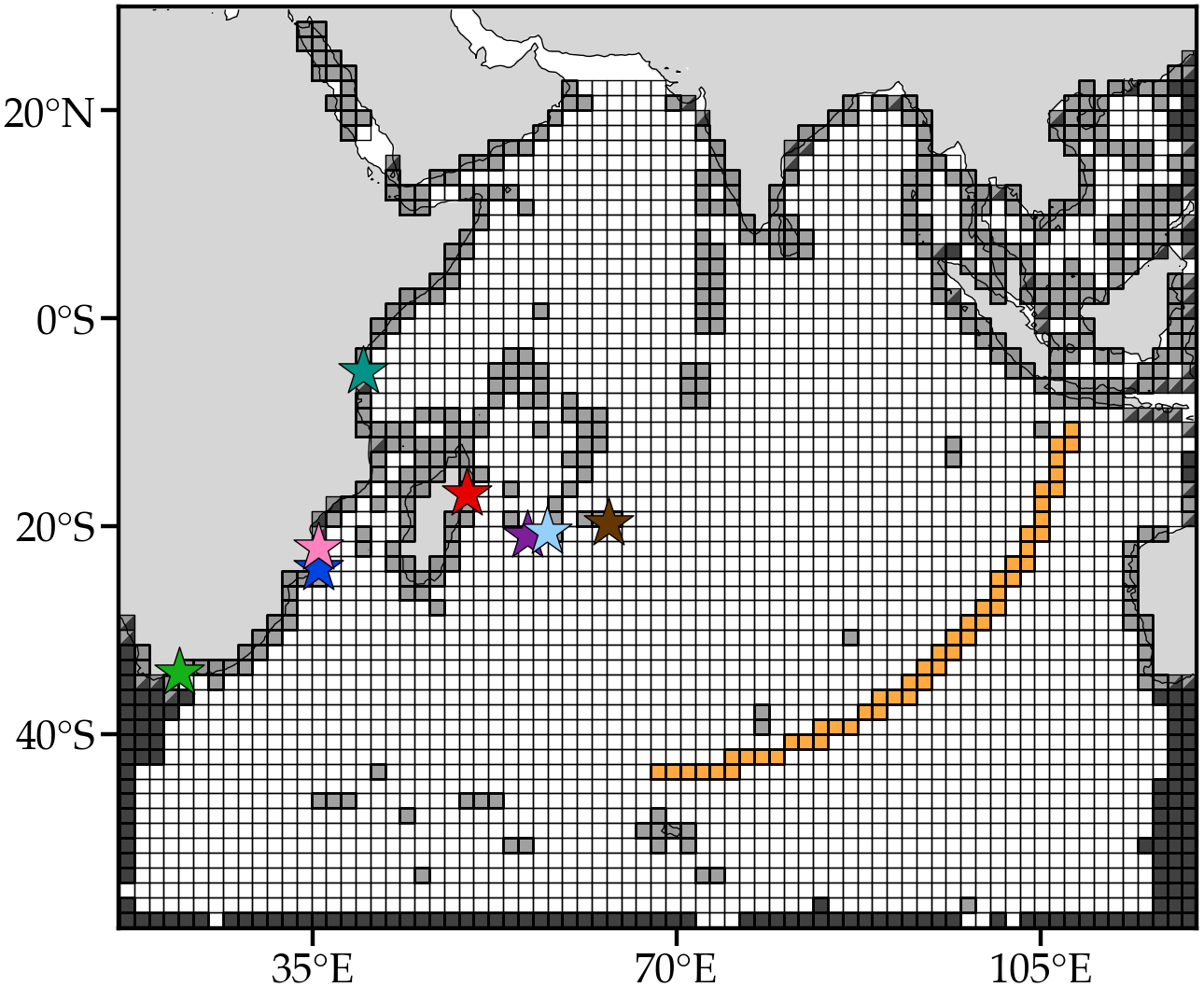
Figure 1: Covering of the Indian Ocean domain into boxes forming the various Markov-chain models constructed using satellite-tracked undrogued drifters to describe the motion of marine debris produced by the crash of Malaysian Airlines flight MH370. Boxes with positive probability of the chain(s) to terminate outside the domain (leaky states) are indicated in dark gray, boxes including land–water interfaces (sticky states) are shown in light gray, and boxes along an arc of 7th ping ring around the Inmarsat-3F1 satellite position when communication with the MH370 flight was lost (crash states) are highlighted in yellow. Stars correspond to the airplane debris beaching sites in Table 1.

To construct $P$, we cover the Indian Ocean domain with a grid of 0.25^∘ $\times$ 0.25^∘ longitude–latitude boxes (Fig. 1). The size of the cells was selected to maximize the grid’s resolution while each individual box is sampled by enough trajectories. Similar grid resolutions in analysis involving buoy trajectory data were employed in recent work Miron et al. (2017, 2018); Olascoaga et al. (2018), where sensitivity analyses to cell size variations and data amount truncations are presented. The area of the boxes varies from about 400 to 750 km², yet the normalization by box area in the definition of the vector space $V_{N}$ makes this variation inconsequential, i.e., a stochastic transition matrix is obtained without the need of a similarity transformation (e.g., Froyland and Padberg Froyland and Padberg (2009)). Ignoring time, there are 226 drifters on average per box (cf. Fig. S1 in the Supplementary Material); the number of drifters vary between 36 and 58 if the data are grouped according to season of the year. Equation (3) is then evaluated for appropriate transition time ($T$) and time-homogeneity interval ($\mathfrak{T}$) choices.

Using $T=1$ d, approximately the surface ocean Lagrangian decorrelation time LaCasce (2008), the simple Markovian dynamics test $\lambda(P(nT))=\lambda(P(T))^{n}$, where $\lambda$ denotes eigenvalue, holds very well up to $n=10$ (cf. Fig. S2 in the Supplementary Material). Here we have chosen to use $n=5$ (equivalently $T=5$ d) as this guarantees both good interbox communication and negligible memory into the past. Similar choices have been made in recent applications involving drifter data Maximenko, Hafner, and Niiler (2012); Miron et al. (2017); McAdam and van Sebille (2018); Miron et al. (2018); Olascoaga et al. (2018).

The simplest choice for the time-homogeneity interval $\mathfrak{T}$ is one that coincides with the entire record of trajectory data Maximenko, Hafner, and Niiler (2012); Miron et al. (2017); McAdam and van Sebille (2018); Miron et al. (2018); Olascoaga et al. (2018). The resulting autonomous Markov chain, which will be only considered for comparison purposes, ignores any mode of variability of the ocean circulation and thus is not optimal for describing debris motion in seasonally dependent environments like the Indian Ocean.

Different $\mathfrak{T}$ intervals can be considered (e.g., van Sebille et al. van Sebille, England, and Froyland (2012)) to represent the dominant variability mode of the Indian Ocean circulation, produced by seasonal changes in the wind stress associated with the Indian monsoon Schott and McCreary, Jr. (2001). During the northern winter, when the monsoon blows southwestward, the flow of the upper ocean is directed westward from near the Indonesian Archipelago to the Arabian Sea. During the northern summer, with the change of the monsoon direction toward the northeast, the ocean circulation reverses, with eastward flow extending from Somalia into the Bay of Bengal. Thus we consider three $\mathfrak{T}$ intervals: January–March ($\mathfrak{T}_{\mathrm{W}}$), which typically corresponds to the winter monsoon season, July–September ($\mathfrak{T}_{\mathrm{S}}$), corresponding to the summer monsoon season, and April–June and October–December together ($\mathfrak{T}_{\mathrm{SF}}$), seasons which do not need to be distinguished from one another to represent the monsoon-induced circulation of the Indian Ocean. This results in three transition matrices, $P_{\mathrm{W}}$, $P_{\mathrm{S}}$ and $P_{\mathrm{SF}}$, respectively, which are appropriately considered for $t\in\mathfrak{T}_{\mathrm{W}}$, $\mathfrak{T}_{\mathrm{S}}$ or $\mathfrak{T}_{\mathrm{SF}}$, when a probability vector is evolved (pushed forward) under left multiplication. We will refer to the resulting Markov-chain model as nonautonomous.

Finally, if the interest is in the fate of the debris in the seasonally changing Indian Ocean environment after several years, one can more conveniently push forward probabilities using a $P$ constructed by combining the above seasonal $P$s in such a way that the resulting Markov chain has a transition time $T$ of 1 yr. Recalling that $T=5$ d for the seasonal $P$s, this is (approximately) achieved by $P=P_{\mathrm{W}}^{18}\cdot P_{\mathrm{SF}}^{18}\cdot P_{\mathrm{S}}^{18}\cdot P_{\mathrm{SF}}^{18}$. The resulting Markov-chain model will be referred to as autonomous season-aware. Similar constructions have been considered earlier (e.g., Froyland et al. Froyland, Stuart, and van Sebille (2014)).

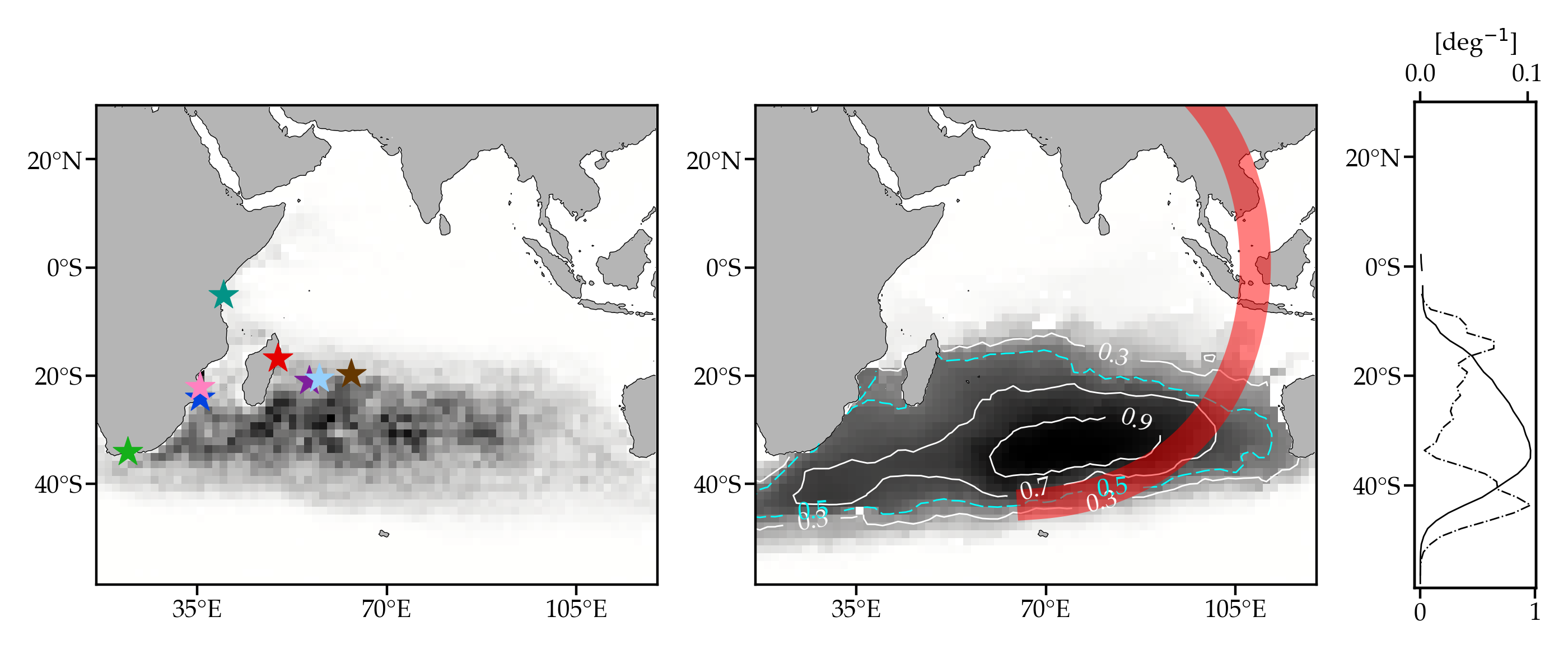
Figure 2: (left) Dominant left eigenvector of the autonomous season-aware transition matrix with beaching sites indicated (cf. Table 1). (middle) Dominant right eigenvector with the Inmarsat arc overlaid. (right) Zonally averaged right eigenvector (solid, bottom axis) and its derivative (dashed, top axis). Local maxima in the left eigenvector are regions that attract trajectories which tend to run long there before exiting the Indian Ocean. The basin of attraction roughly corresponds to the region enclosed by the 0.5 right eigenvector level set, above which the eigenvector looks closer to $\mathbf{1}$.

IV Crash site assessment from spectral analysis

Information about the long-time asymptotic behavior of a dynamical system described by an autonomous transition matrix $P$ can be obtained from its spectral properties Hsu (1987); Dellnitz and Junge (1999); Froyland (2005). Indeed, the leading eigenvector structure of $P$ suggests a dynamical partition or geography Froyland, Stuart, and van Sebille (2014); Miron et al. (2017, 2018) of weakly interacting sets that constrains connectivity between distant points in phase space. Here we unveil such a dynamical geography from the autonomous season-aware Markov chain to gain insight into debris motion and thus the crash site.

For any irreducible and aperiodic stochastic $P$, its dominant left eigenvector, $\mathbf{p}$, satisfies $\mathbf{p}P=\mathbf{p}$ and (scaled appropriately) represents a limiting invariant or stationary distribution, namely, $\mathbf{p}=\smash{\lim_{k\uparrow\infty}\mathbf{f}P^{k}}$ for any probability vector $\mathbf{f}$ (cf., e.g., Horn and Johnson Horn and Johnson (1990)). Also, $\mathbf{1}=P\mathbf{1}$, where $\mathbf{1}$ denotes the vectors of ones, is the right eigenvector corresponding to the eigenvalue 1 and $\mathbf{p}$.

If $P$ is substochastic, i.e., $\smash{\sum_{j}}P_{ij}<1$ for some $i$, the dominant left eigenvector $\mathbf{p}\geq 0$ decays at a rate set by the dominant eigenvalue $\lambda_{1}<1$, and has the interpretation of a limiting almost-invariant or quasistationary distribution, namely, the limiting distribution of trajectories that run long before terminating (cf. Chapter 6.1.2 of Bremaud Brémaud (1999)). Restricted to the set $B$ where those trajectories start, i.e., the basin of attraction, the dominant right eigenvector is close to $\mathbf{1}$ Koltai (2011); Froyland, Stuart, and van Sebille (2014); Miron et al. (2017, 2018).

The left and middle panels of Fig. 2 show respectively the dominant left ($\mathbf{p}$) and right ($\mathbf{r}$) eigenvectors of the autonomous $P$ introduced in the preceding section. The right panel in turn shows again the right eigenvector, but this time zonally averaged (solid, bottom axis), along with its (meridional) derivative (dashed, top axis), which maximizes near the 0.5 level set. The dominant eigenvalue $\lambda_{1}=0.8181$ sets an annual decay rate for $\mathbf{p}$ of about 20%, which is nearly four times slower than that experienced by the first subdominant left eigenvector ($\lambda_{2}=0.4012$). Note the structure of $\mathbf{p}$, taking many local maxima toward the western side of Indian Ocean, inside the 20–40^∘S band. The right eigenvector is much less structured, looking closer to $\mathbf{1}$ within the region enclosed by the 0.5 level set. This region approximately forms a basin of attraction $B=\{\mathbf{r}>0.5\}$ for trajectories that asymptotically distribute as $\mathbf{p}$ conditional to staying in the domain for a long time.

The expected retention time in $B$ is given by $T_{B}=T/(1-\lambda_{B})$, where $\lambda_{B}$ is the dominant eigenvalue of $P$ restricted to $B$ (cf. Appendix B of the Supplementary Material for a derivation and Miron et al. Miron et al. (2018) for a recent application). We compute $\lambda_{B}=0.5103$, and noting that $T=1$ yr for the autonomous season-aware $P$, we estimate $T_{B}=2.0421$ yr, which is of the order of the mean time it took observed airplane debris to reach the African coasts (cf. Table 1). This long residence time and the large area spanned by $B$ impose a constraint on the connectivity between locations in- and outside of $B$ by debris trajectories, which we use to make an initial assessment of the possible crash site as follows.

Note in the left panel of Fig. 2 that the observed beaching sites (stars) lie within or the border of the western region where $\mathbf{p}$ tends to locally maximize. Note in the middle panel that the Inmarsat arc traverses the eastern side of $B$. This suggests a possible crash site somewhere along the Inmarsat arc sector between the latitudes of intersection with of $B$, roughly 20 and 40^∘S.

In the next sections we will show that the uncertainty (about 3600 km) of the spectral assessment above can be substantially reduced using a dedicated Bayesian analysis along with the computation of most probable paths and the inspection of a particular drifter trajectory.

V Bayesian estimation of the crash site

The Bayesian analysis uses the beaching events as observations to infer the probability distribution of the crash site (refer to Appendices C and D in the Supplementary Material for mathematical details). Because of the shorter-time nature of these observations, the analysis is most appropriately carried out using the nonautonomous Markov-chain model, albeit with some convenient adaptation.

As our computational domain is not the whole ocean, necessarily trajectories can leave the domain, and not have an assignable termination box. For example, the Agulhas Current transports approximately 70 Sv (1 Sv $=10^{6}$ m³s^-1) out of the western boundary of the domain Beal et al. (2011). This leakage is represented by $\smash{\sum_{j}}P_{ij}<1$ for the leaky states $i\in\mathfrak{L}\subset S:=\{1,\dotsc,N\}$ (black boxes in Fig. 1). (Herein $P$ is any $P_{\mathrm{W}}$, $P_{\mathrm{S}}$ or $P_{\mathrm{SF}}$, which are applied for $t\in\mathfrak{T}_{\mathrm{W}}$, $\mathfrak{T}_{\mathrm{S}}$ or $\mathfrak{T}_{\mathrm{SF}}$ as appropriate.) To account for the leakage and retain the open dynamics nature of the Indian Ocean, we introduce an absorbing state $N+1$, commonly referred to as cemetery state, and consider $1-\smash{\sum_{j}}P_{i\in\mathfrak{L},j}$ to be the probability of the chain to move and terminate in it, if currently being in state $i\in\mathfrak{L}$. This amounts to augmenting $P\in\mathbb{R}^{N\times N}$ to $P\in\mathbb{R}^{(N+1)\times(N+1)}$ by

$$\begin{cases}P_{i\in\mathfrak{L},j=N+1}\leftarrow 1-\sum_{j}P_{i\in\mathfrak{L},j},\\ P_{i=N+1,i}=1,\end{cases}$$ (5)

satisfying $\sum_{j}P_{ij}=1$.

In addition to the dynamics being open, as we are considering floating debris which might come ashore somewhere, the transition matrix has to account for the Markov chain possibly terminating on water–land interfaces. Such events are hard to identify from the dataset because drifters can terminate for multiple reasons (e.g., malfunction, recovery, end of life). To account for beaching, we identify the set of sticky states $\mathfrak{S}\subset S$ (grey boxes in Fig. 1) with those coastal boxes that contain land–water interfaces and introduce the land fraction function $\ell:\mathfrak{S}\to(0,1)$. Note that a sticky state may also be leaky, namely, $\mathfrak{S}\cap\mathfrak{L}$ need not be empty. We then denote by $\mathfrak{D}\subset\mathfrak{S}$ the subset of sticky boxes where airplane debris were found to beach, to distinguish them from the others. Beaching is then modeled by augmenting $P\in\smash{\mathbb{R}^{(N+1)\times(N+1)}}$ to $P\in\smash{\mathbb{R}^{(N+1+M)\times(N+1+M)}}$, satisfying $\sum_{j}P_{ij}=1$ and where $M=|\mathfrak{D}|(=8)$, according to:

$$\begin{cases}P_{i\in\mathfrak{S},j\in S\cup\{N+1\}}\leftarrow(1\!-\!\ell(i\!\in\!\mathfrak{S}))P_{i\in\mathfrak{S},j\in S\cup\{N+1\}},\\ P_{i\in\bar{\mathfrak{S}},j=N+1}\leftarrow\ell(i\!\in\!\bar{\mathfrak{S}})+(1\!-\!\ell(i\!\in\!\bar{\mathfrak{S}}))P_{i\in\bar{\mathfrak{S}},j=N+1},\\ P_{i\in\mathfrak{D},j=N+1+m(i\in\mathfrak{D})}=\ell(i\!\in\!\mathfrak{D}),\\ P_{i\in N+1+m(\mathfrak{D}),i}=1,\end{cases}$$ (6)

where $\bar{\mathfrak{S}}:=\mathfrak{S}\setminus\mathfrak{D}$, $m:\mathfrak{D}\to\{1,\dotsc,M\}$, and $N+1+m(i\in\mathfrak{D})$ represents a target cemetery state where the chain terminates whenever beaching from $i\in\mathfrak{D}$. The first line in (6) deals with sticky boxes if the chain flows on. The second line deals with sticky but nondebris beaching boxes, each of which also is terminated in the cemetery state ($N+1$). The third line deals with debris-beaching boxes if the chain terminates from them by beaching. Finally, the fourth line makes each target cemetery state absorbing.

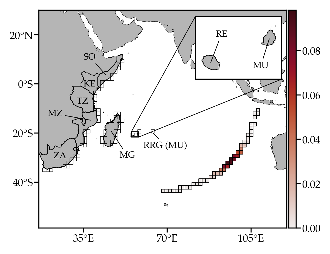
Figure 3: Posterior probability of the crash site, for given assumed mutually independent observations of debris beaching time and based on the nonautonmous Markov-chain model. Indicated are countries and territories in the western side of the Indian Ocean domain and corresponding boxes of the domain covering. Acronyms SO and KE stand for Somalia and Kenya, respectively; cf. Table 1 for the rest of the acronyms.

Having settled on an appropriate $P$ representation, we proceed to formulate the Bayesian estimation problem by first fixing some notation. Let $\mathfrak{C}\subset S$ denote the set of indices of the boxes (states) along the Inmarsat arc—the possible crash sites. We call $b$ a state in the set $\mathfrak{B}:=\{N+2,\dotsc,N+M+1\}$ of airplane debris beaching site boxes and further make $\mathbf{b}:=(b)_{b\in\mathfrak{B}}\in\mathbb{N}^{M}$. Let $\{\xi_{t+kT}\}_{k\geq 0}$ be time-discrete random position variables that take values on the augmented Markov chain states $S\cup\{N+1\}\cup\mathfrak{B}$, and $t$ denotes the crash time, when the chain starts. Consider then the random variable $\tau^{b}$ denoting the time after which the chain gets absorbed into a particular beaching state $b$, namely,

$$\tau^{b}:=\inf_{k\geq 0}\{t+kT:\xi_{t+kT}=b\in\mathfrak{B}\}.$$ (7)

Define $\mathop{\rm prob}\nolimits_{c}[\cdot]:=\mathop{\rm prob}\nolimits[\,\cdot\mid\xi_{t}=c\in\mathfrak{C}]$ and

$$p_{c}^{b}(k):=\mathbf{1}_{c}P^{k}\cdot\mathbf{1}_{b},\quad c\in\mathfrak{C},\,b\in\mathfrak{B},$$ (8)

where $\mathbf{1}_{j}=(\delta_{ij})_{i\in S\cup\{N+1\}\cup\mathfrak{B}}$, and then note that

$$\mathop{\rm prob}\nolimits_{c}[\tau^{b}=t+kT]=\begin{cases}p_{c}^{b}(k)=0&\text{if }k=0,\\ p_{c}^{b}(k)-p_{c}^{b}(k-1)&\text{if }k>0.\end{cases}$$ (9)

Let us now assume that after the crash every single piece of debris was transported mutually independently. For each debris, we have access to two observations of random quantities: the beaching site and the beaching time. Let $\xi$ and $\tau$ denote these random variables, respectively, and note that if the target is absorbing, then $\tau^{b}<\infty$ from (7) implies $\xi=b$, and thus the events $\{\xi=b\text{ and }\tau=t^{b}\}$ and $\{\tau^{b}=t^{b}\}$ are equivalent. Thus the joint probability of these observations, i.e.,

$$p(t^{b}|c):=\mathop{\rm prob}\nolimits_{c}[\tau=t^{b}\text{ and }\xi=b]\equiv\mathop{\rm prob}\nolimits_{c}[\tau^{b}=t^{b}],$$ (10)

is computable as in (9). The probabilities $p(t^{b}|c)$ depend on the crash site $c$. Now, making use of the independence assumption above, the joint probability of the observations, given the crash site $c$, is

$$p(t^{\mathbf{b}}|c):=\prod_{b\in\mathfrak{B}}p(t^{b}|c).$$ (11)

The idea of Bayesian inversion Bolstad and Curran (2016) is to find a probabilistic characterization of the unknown parameter $c$ (crash site) given the debris beaching times and locations. By viewing $p(t^{\mathbf{b}}|c)$ as a function of $c$, one obtains a function $L(c;t^{\mathbf{b}})$ which represents the likelihood of $c$. The posterior distribution of $c$, i.e., the probability distribution of $c$ once $t^{\mathbf{b}}$ have been observed, follows from Bayes’ theorem:

$$p(c|t^{\mathbf{b}})\propto p(t^{\mathbf{b}}|c)\cdot p(c),$$ (12)

where $p(c)$ is the prior distribution of $c$, representing the state of knowledge about $c$ before to data have been observed.

Assuming that $p(c)$ is uniform (i.e., maximally uninformative) over $\mathfrak{C}$, the Inmarsat arc boxes, Fig. 3 shows $p(c|t^{\mathbf{b}})$ for debris beaching times $t^{\mathbf{b}}$ as given in Table 1. The maximum likelihood estimator, $c_{\mathrm{max}}=\operatorname*{arg\,max}_{c}p(t^{\mathbf{b}}|c)$, corresponds to the index of the Inmarsat arc box centered at about 31^∘S. To check how reasonable this crash site estimate is, the top panel of Fig. S3 in Appendix F of the Supplementary Material shows that the joint probability $\mathop{\rm prob}\nolimits_{c_{\mathrm{max}}}[\tau=t+kT\text{ and }\xi_{t+kT}=s]$ for each sticky state $s\in\mathfrak{S}$ tends to maximize near the observations. The misfit is attributed to the historical drifter data not capturing all of the details of the Indian Ocean dynamics and in particular those when the crash took place and the years after it. For instance, the bottom panel of Fig. S3 shows that the misfit augments when the monsoon variability is ignored.

The Bayesian crash site estimate, 31^∘S on the Immarsat arc, lies within the arc portion identified as a likely crash region using the spectral analysis of the previous section. An important difference is that the uncertainty of the assessment is constrained by the Bayesian analysis. For instance, the 95%  central posterior interval length, obtained by computing the 2.5 and 97.5%-ile of the posterior distribution, is of about 12^∘ along the arc, which is nearly twice as narrow as the spectral inference. However, the Bayessian inference is affected by a bimodality in the single posterior distributions of the crash site. This is demonstrated in Fig. 4, which shows $p(c|t^{b})$ plotted for each $b\in\mathfrak{B}$ individually as a function of the latitude of $c\in\mathfrak{C}$. These can be collected into two quite consistent groups. Specifically, a southern group, which favors a most likely crash site near $36^{\circ}$S on the arc, and a northern group, favoring a most likely position near $25^{\circ}$S.

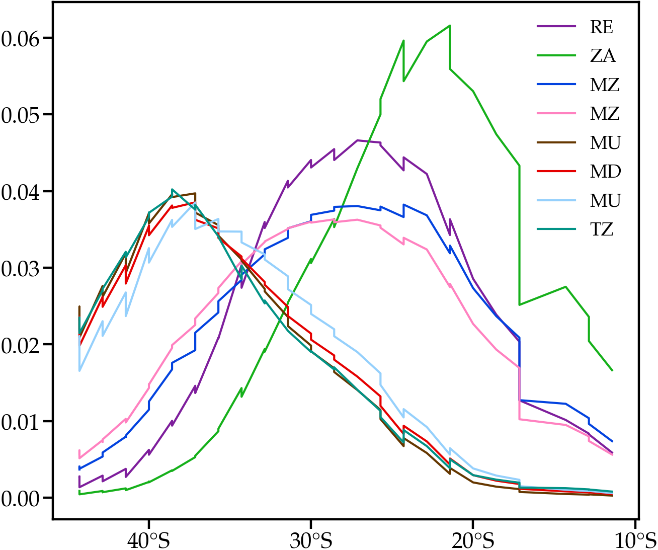
Figure 4: Single posterior distributions of the latitude of the crash site along the Inmarsat arc, computed using the nonautonmous Markov-chain model. Refer to Table 1 for acronym meanings.

VI Narrowing the uncertainty of the crash site determination

We close the analysis by discussing one additional calculation and a particular observation that altogether provide means for favoring the northern of the above two possible crash sites, improving the confidence of its determination.

Drifter data does not merely give the chance to construct a Markov chain model of the surface currents, but also to study single trajectories. Thus we consider the most probable paths of our model that end up at the particular beaching sites. More precisely, as we know how long (in time) the single trajectories were, we compute most probable paths ending at a given beaching site $b\in\mathfrak{B}$ after having ran for a fixed time $t^{b}$. The basic idea of the process is to set up and iteratively solve a dynamical programming equation relating the maximal probability of a path reaching some state $i\in S$ after exactly $t+T$ units of time with the maximal probabilities of paths reaching other states $j\in S$ after $t$ (cf. Appendix E in the Supplementary Material for details as well as for a review of standard unconstrained extremal path notions Dijkstra (1959); Floyd (1962)). It is important to realize that the probability of single paths is extremely low (as there are so many possible ones), and the most probable one can sensitively depend on the slightest variations of the dynamics. Thus they are only suitable for qualitative comparisons with observations. We note that constrained paths were considered to analyze currents in the Mediterranean Sea by Ser-Giacomi et al. Ser-Giacomi et al. (2015), yet without excluding the possibility to hit the target before the end time.

The result is shown in Fig. 5, revealing, on the one hand, quite remarkably that the most probable paths of different fixed lengths (dotted curves) start from a common box that is the Inmarsat arc box centered at roughly (105^∘E, 16^∘S). On the other hand, Triñanes et al. Trinanes et al. (2016) report on a drifter (ID 56568, from the NOAA/GDP database) that crossed the Inmarsat arc near (103^∘E, 22^∘S) in March 2014 and after looping for a little while about the arc near (102^∘E, 25^∘S) reached the vicinity of Reunion Island in July 2015, about the time when the first MH370 debris piece was spotted. The trajectory of the drifter in question is shown in gray in Fig. 5.

Taken together, the most probable path computation and the specific drifter trajectory observation favor the Bayesian crash site estimate near 25^∘. Excluding from the Bayesian analysis the debris beaching data that leads to single posterior crash site distributions peaking near $36^{\circ}$S, we estimate a 95%  central posterior interval length of 16^∘ along the Inmarsat arc for the refined crash site inference.

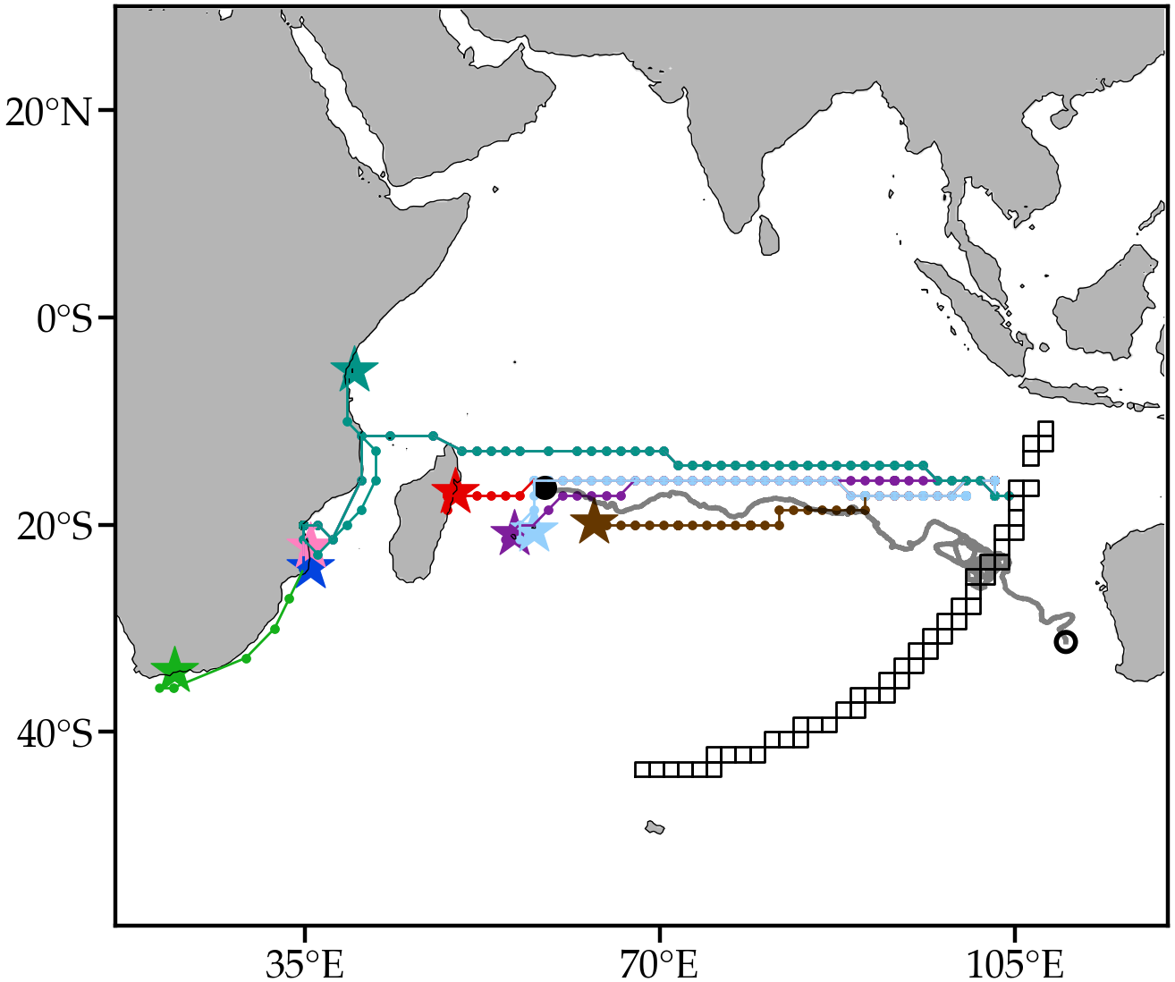
Figure 5: Most probable paths (dotted) along the nonautonomous Markov chain between Inmarsat arc boxes and each of the debris beaching sites (cf. Table 1), and trajectory (gray) of a NOOA/GDP drifter (ID 56568) launched west of the Australian coast.

We finally note that the qualitative assessment in this section, along with the spectral analysis assessment, provide a guideline to construct a prior distribution that can be incorporated to the Bayesian analysis. More specifically, these assessments suggest an informative prior distribution narrowing near 25^∘N on the Inmarsat arc.

VII Summary and concluding remarks

Using historical satellite-tracked surface drifter data in the Indian Ocean, we have proposed a Markov-chain model representation of the drift of observed marine debris from the missing Malaysian Airlines flight MH370.

The results from a spectral analysis of an autonomous discrete transfer operator (transition matrix) that controls the long-term evolution of the debris in a seasonally changing environment showed that the crash region is likely restricted to the 20–40^∘S portion of the arc of the 7th ping ring around the Inmarsat-3F1 satellite position when the airplane lost contact on 8 March 2014. The solution of a dedicated Bayesian estimation problem that uses the locations and times of confirmed airplane debris beachings in a Markov-chain model defined by a nonutonomous transition matrix capable of resolving shorter-term details of the debris evolution, further identified two probable crash sites within the aforementioned arc portion, one near $36^{\circ}$S and another one near $25^{\circ}$S. Consideration of most probable paths between the Inmarsat arc and the debris beaching sites constrained by the observed (elapsed) beaching times, and the observation of a drifter that took a trajectory similar to the path connecting the arc and the Reunion Island beaching site, was shown when taken together to favor the 25^∘S crash site estimate.

Our Bayesian crash site estimate, with a 95%  central posterior interval ranging from 33 to 17^∘S on the Inmarsat arc, is consistent with the most recently published Nesterov (2018) crash area estimate, 28–30^∘ along the arc, but it lies north of the latest recommended search area by the Commonwealth Scientific and Industrial Research Organisation Griffin, Oke, and Jones (2017), at around 35^∘S. Notwithstanding, it is consistent with the original northern definition of high-priority search zone by the Australian Transport Safety Bureau Australian Transport Safety Bureau .

The uncertainty of our crash site estimate may be attributed to unresolved nonautonomous dynamical effects by the Markov-chain model constructed from the historical drifter data. Indeed, the historical drifter data may fall short of capturing all of the details of the circulation (e.g., at the submesoscale), particularly during the years after the crash took place. Moreover, undrogued drifter motion, while different than water parcel motion, may not accurately represent the motion of airplane debris pieces with varied shapes and thus drag properties.

While our results may provide grounds for guiding search efforts, currently halted, the operational use of the probabilistic framework proposed here in such a task will require one to consider an appropriate data-assimilative system. Indeed, the probabilistic framework may well be applied on observed trajectory data, as we have chosen to do in this paper, or on numerically generated trajectory data. Clearly, the success of such an operative use of the framework will depend on the operator’s ability to appropriately modeling the effects of the inertia of the debris pieces (i.e., of their buoyancy, size and shape), which is a subject of active research Cartwright et al. (2010); Beron-Vera et al. (2015); Beron-Vera, Olascoaga, and Lumpkin (2016).

We finally note that the framework here presented is well-suited for inverse modeling in a general setting and thus its utility is far reaching. Such modeling is critical, for instance, in contamination source backtracking Bagtzoglou and Atmadja (2005). Relevant oceanic problems include that of red tide early development tracing Olascoaga et al. (2008) and oil spill source detection Gautama et al. (2016). In the atmosphere, examples for instance are the identification of sources of greenhouse gases emission Hourdin and Talagrand (2006) and toxic agents release Rao (2007).