Density shocks in the relativistic expansion of highly charged one component plasmas

Abstract

In a previous paper we showed that dynamical density shocks occur in the non-relativistic expansion of dense single component plasmas relevant to ultrafast electron microscopy; and we showed that fluid models capture these effects accurately. We show that the non-relativistic decoupling of the relative and center of mass motions ceases to apply and this coupling leads to novel behavior in the relativistic dynamics under planar, cylindrical, and spherical symmetries. In cases where the relative motion of the bunch is relativistic, we show that a dynamical shock emerges even in the case of a uniform bunch with cold initial conditions; and that density shocks are in general enhanced when the relative motion becomes relativistic. Furthermore, we examine the effect of an extraction field on the relativistic dynamics of a planar symmetric bunch.

I Introduction

The expansion dynamics of highly charged plasmas is a fundamental problem in areas ranging from astrophysics to nanotechnology to beam physics. Previous analytic work has focused on initial conditions where a highly charged plasma is cold and has uniform densityJansen (1988); Reiser (1994); Batygin (2001); Bychenkov and Kovalev (2005); Grech et al. (2011); Kaplan et al. (2003); Kovalev and Bychenkov (2005); Last et al. (1997); Eloy et al. (2001); Krainov and Roshchupkin (2001); Morrison and Grant (2015); Boella et al. (2016); Bychenkov and Kovalev (2011) However, the vast majority of this work, with the exception of Bynchenkov and KovalevBychenkov and Kovalev (2011), have assumed non-relativistic conditions. In ultrafast electron microscopy (UEM) and some beam physics applications, electron sources are used to produce dense bunches of charged particles within an intense extraction field that is used to accelerate the distribution to near-luminal speeds. In addition, for sufficient densities, the bunch self-field can result in relativistic velocities within the frame of the bunch. These concerns indicate that a relativistic theory is required in many practical cases, and here we present the relevant theory.

The typical analytic approach to relativistic expansion dynamics of such systems is a treatment based on envelope equations that are predicated on the conservation of emittance and the use of uniform density distributionsReiser (1994). Uniform ellipsoidal distributions are particularly amenable to analysis as the self-electrostatic field in these distributions is linear and the expansion dynamics results in a simple power law growth of the ellipsoid axes – at least in the non-relativistic regime. Furthermore, it is fairly straightforward to show that uniform ellipsoids conserve emittance as long as all the particles can be treated as having identical Lorentz factors. Moreover, analysis of beam dynamics such as emittance oscillationAnderson (1987), emittance compensationRosenzweig et al. (2006), and the beam halo Gluckstern (1994) generally assume similar uniform-like conditions. However, for electron injectors utilizing photoemission the initial conditions of the bunch is often Gaussian, or at the very least non-uniform, and it has long been known that charge redistribution from the non-uniform to the uniform bunch is one of the major sources of emittance growthWangler (1991) suggesting that uniform distributions are at best an idealization that miss much of the physics present in the typical situation. However, we have recently shown that dynamics similar to Wangler’s charge redistribution for freely expanding bunches leads to an opportunity of “Coulomb cooling” — a mechanism we believe employs the intense Coulomb fields to carry off heat from non-neutral plasmasWilliams et al. (2017); Zerbe et al. (2018). Our analysis is directed at a better understanding of the relativistic expansion dynamics of uniform and non-uniform systems to study mechanisms of emittance growth near the particle source but also with the goal of understanding and optimizing Coulomb cooling. Here we concentrate on characterizing the relativistic density dynamics for both uniform and non-uniform initial conditions.

Numerous works within the UEM literature have already looked at various aspects of the evolution of non-uniform distributionsDegtyareva et al. (1998); Luiten et al. (2004); Musumeci et al. (2008); Morrison et al. (2013); Li and Lewellen (2008); Siwick et al. (2002); Qian and Elsayed-Ali (2002); Reed (2006); Collin et al. (2005); Gahlmann et al. (2008); Tao et al. (2012); Portman et al. (2013, 2014); Michalik and Sipe (2006); Zerbe et al. (2018). Reed presented a fluid model that described the dynamics of non-uniform bunch expansion under the assumptions that the bunch could be treated as having planar symmetry in the non-relativistic regimeReed (2006). In our previous paperZerbe et al. (2018), we showed that the expansion dynamics in the planar case differs greatly from symmetries in higher dimensions and verified analytic description of the dynamics utilizing both N-particle and particle-in-cell (PIC) simulations. The analytic descriptions depend on terms that can be written as functions multiplied by the quantity

$$D_{01}=\frac{{\bar{\rho}}_{01}}{\rho_{01}}-1$$ (1)

for planar geometries or by the quantity

$$D_{0d}=\frac{\rho_{0d}}{{\bar{\rho}}_{0d}}-1$$ (2)

for cylindrical ($d=2$) and spherical ($d=3$) geometries, where $\rho_{0d}$ is the initial density at location $r_{0}$ and ${\bar{\rho}}_{0d}$ is the average density within that location. For the uniform distribution, the local density and the average density are the same so that $D_{0d}=0$ everywhere and the density evolution’s dependence on the aforementioned functions vanishes reducing the dynamics to the uniform dynamics utilized extensively in the literature. Otherwise, these functions play a large role in the density evolution leading to differences in the dynamics of distributions with different initial density profiles. Specifically, we showed that a density shock, seen in Coulomb explosion studiesGrech et al. (2011); Kaplan et al. (2003); Kovalev and Bychenkov (2005); Last et al. (1997); Murphy et al. (2014); Reed (2006); Degtyareva et al. (1998), was present in the analytic density evolution of initially Gaussian distributions under both cylindrical and spherical symmetries but absent under planar symmetry unless an appropriate initial chirp in phase space is present. Moreover, such a shock is absent in non-relativistic dynamics of uniform systems with cold initial conditions suggesting that uniform distribution evolution is unique in this regardZerbe et al. (2018).

We noted in our previous work that the density evolution seen in PIC simulations using an electromagnetic (EM) solver and relativistic particle pusher, which should capture all relativistic effects if the initial field is accurate, do not significantly differ from our analytic description for the densities analyzed thereZerbe et al. (2018). Moreover, we have seen that the PIC simulations using an EM solver do not significantly differ from those using an electrostatic (ES) solver with relativistic particle pusher for much higher densities than those examined in our previous work, or in the work described here. Assuming the accuracy of the initial fields, we conclude that the relativistic effects are then adequately captured within the relativistic particle pusher, which is equivalent to simply including the relativistic momentum in the analysis. Precisely such an analysis of the relativistic free-expansion of a spherically-symmetric, cold uniform charge distribution was completed by Bychenkov and KovalevBychenkov and Kovalev (2011), and part of what we do in this manuscript is extend this analysis to non-uniform cases as well as additional symmetries.

Here we treat charge distributions with general initial spatial distributions starting from rest under planar, cylindrical and spherical geometries introducing a novel length scale that is associated with each symmetry. First in Section II.1, we present general results applicable to all cases. In Section II.2 we derive expressions for planar symmetry for any arbitrary initial spatial distribution and examine these expressions in the non-relativistic and highly relativistic limits. We then introduce $M$-shell simulations, which are simulations of $M$ equally charged planes in 1D, and show that these simulations reproduce the density evolution derived analytically. In Sections II.3 and II.4, we derive relativistic density evolution expressions under cylindrical and spherical symmetries, respectively, for arbitrary initial distributions, and we show that these expressions are consistent with PIC calculations using an EM solver and relativistic particle pusher utilizing the well-known package warpFriedman et al. (2014). Further, we show that $M$-shell simulations, which track $M$ equally charged cylindrical- and spherical- shells in 2- and 3- dimensions, respectively, also capture the same density evolution. We validate these expressions against their non-relativistic and uniform relativistic counterparts, and we examine the expressions in the highly relativistic limit.

In Section III we introduce an external extraction field in the case of a planar electron bunch, and we point out that the acceleration from self-fields and external fields do not decouple in the relativistic case. Though the analysis is captured by a straightforward extension of the analysis used for the planar case with no extraction field, the physical effects are quite interesting and relevant to ultrafast electron microscopy. In Section IV, we demonstrate how to apply the time dependent distributions to calculate the statistical width of the distribution. Section V contains discussions and conclusions; noting in particular the emergence of density shocks due to relativistic effects, even in planar uniform systems where a shock does not emerge in the non-relativistic limit.

II Relativistic density evolution

In this section we consider planar, cylindrical and spherical geometries in the case of cold initial conditions and where there is no external electromagnetic field. We treat the dynamics using the relativistic treatment of momentum and energy, however we treat the forces between electrons using electrostatics. We then check the latter approximation under cylindrical and spherical geometries using PIC calculations using a full EM solver and find excellent agreement. We start with a general analysis and then specialize in the later three subsections.

II.1 General considerations

II.1.1 General formulation

We consider cold symmetric initial charge distributions so that the electric field at position $z_{0}$ in a planar geometry is given by,

$$E_{0}(z_{0})=E_{01}=\frac{\Sigma_{tot}P_{01}}{2\epsilon_{0}}=E_{T1}P_{01}$$ (3)

where $\Sigma_{tot}=Nq/A$, with $A$ the pulse area, $N$ the number of particles in the bunch, $q$ the charge of each particle, $E_{T1}=\frac{\Sigma_{tot}}{2\epsilon_{0}}$ is the total planar field produced by the particles, and $P_{01}$ is a position specific scalar representing the fraction of the electrons in the bunch contributing to the net electric field on the particle at position $z_{0}$. The physical significance of the total field $E_{T1}$ will be discussed in detail in Section III. The direction along which the charge density varies is $z$, and we assume the initial charge distribution is symmetric about the origin for the sake of simplicity. We define $\rho_{1}(z;t)$ to be the number density per unit length at position $z$ and $\rho_{01}=\rho_{01}(z_{0})=\rho_{1}(z_{0};t=0)$ to be the initial number density at position $z_{0}$. As the initial density $\rho_{01}$ is symmetric about the origin, the cumulative probability is given by,

$$P_{01}=P_{01}(z_{0})=\int_{0}^{z_{0}}2\rho_{01}(z)dz$$ (4)

Notice that the quantity $\Sigma_{tot}P_{01}$ represents the charge per unit area after integrating the number density per unit length $\rho_{01}$ over the range $[-z_{0},z_{0}]$.

In systems with cylindrical symmetry, we have,

$$E_{0}(r_{0})=E_{02}={\Lambda_{tot}P_{02}\over 2\pi\epsilon_{0}r_{0}}=E_{T2}P_{02}$$ (5)

where $\Lambda_{tot}$ is the total charge per unit length along the cylindrical charge distribution, $E_{T2}=\frac{\Lambda_{tot}}{2\pi\epsilon_{0}r_{0}}$ is the electric field a particle at $r_{0}$ would feel if the entire distribution were distributed cylindrically within $r_{0}$, and $P_{02}$ is the cumulative probability given by,

$$P_{02}=\int_{0}^{r_{0}}2\pi r\rho_{02}(r)dr$$ (6)

where $\rho_{2}(r;t)$ is the number density in two dimensions (number per unit area) and where we define $\rho_{02}=\rho_{02}(r_{0})=\rho_{2}(r_{0};t=0)$. Notice that the quantity $\Lambda_{0}P_{02}$ represents the charge per unit length inside radius $r_{0}$.

In systems with spherical symmetry we have

$$E_{0}(r_{0})=E_{03}={Q_{tot}P_{03}\over 4\pi\epsilon_{0}r_{0}^{2}}=E_{T3}P_{03}$$ (7)

where $Q_{tot}$ is the total charge in the system, $E_{T3}=\frac{Q_{tot}}{4\pi\epsilon_{0}r_{0}^{2}}$ and is the electric field a particle at $r_{0}$ would feel if the entire distribution were distributed spherically within $r_{0}$, and $P_{03}$ is the cumulative probability given by,

$$P_{03}=\int_{0}^{r_{0}}4\pi r^{2}\rho_{03}(r)dr$$ (8)

where $\rho_{3}(r;t)$ is the number density in three dimensions (number per unit volume) and where we define $\rho_{03}=\rho_{03}(r_{0})=\rho_{3}(r_{0};t=0)$. Again notice that $P_{03}$ represents the fraction of the particles that lie inside radius $r_{0}$ and $Q_{tot}P_{03}$ gives the charge inside radius $r_{0}$.

To make analytic progress we make the laminar fluid approximation, which states that there is no mixing of the charged particle trajectories. As a result, the symmetries of the charge distributions are conserved. If we consider a particle of charge $q$ and rest mass $m$ starting from rest (cold initial conditions); at position $z_{0}$ (planar case) or $r_{0}$ (cylindrical or spherical cases), we want to find the position and velocity of the particle at later times. In a planar system we thus want to find $z(z_{0},t)=z$ and $v(z_{0},t)=v$; while in the cylindrical and spherical cases we want to find the radial position and radial velocity $r(r_{0},t)=r$; $v(r_{0},t)=v$. One approach is to use the relativistic form of Newton’s second law,

$$\frac{dp}{dt}=qE$$ (9)

where we are considering the $z$ component of these vectors in planar geometries and the radial component in cylindrical and spherical geometries. We use the relativistic expression for the momentum,

$$p=\gamma mv$$ (10)

where $m$ is the rest mass and

$$\gamma=\frac{1}{\sqrt{1-(\frac{v}{c})^{2}}}$$ (11)

Due to the laminar fluid property, the electric field experienced by a particle at position $z(z_{0},t)$ in planar geometries is the same as the electric field this particle experienced at it’s initial position, so that

$$E_{1}(z)=E_{01}$$ (12)

In cylindrical geometries using Gauss’ law we find,

$$E_{2}(r)=E_{02}\frac{r_{0}}{r}$$ (13)

and analogously in spherical geometries we have,

$$E_{3}(r)=E_{03}\left(\frac{r_{0}}{r}\right)^{2}$$ (14)

These expressions may be used with Newton’s second law to solve for the particle dynamics. Alternatively in an energy formulation, conservation of energy requires that the change in kinetic energy equals the change in potential energy. We use the relativistic form of the kinetic energy,

$$K=(\gamma-1)mc^{2}$$ (15)

and the change in kinetic energy is equal to $K$ as the bunch starts from rest. The change in potential energy is found by integrating the force $qE$, which for the planar case gives,

$$\Delta U_{1}=qE_{01}(z_{0}-z)$$ (16)

while for the cylindrical case we find,

$$\Delta U_{2}=qE_{02}r_{0}\ln\left(\frac{r_{0}}{r}\right)$$ (17)

and for the spherical case,

$$\Delta U_{3}=qE_{03}r_{0}^{2}\left(\frac{1}{r}-\frac{1}{r_{0}}\right)$$ (18)

Notice that $\Delta U\leq 0$ for all time due to the physics as the potential energy decreases as the electron bunch expands. Setting the sum of the changes in potential and kinetic energy to zero, we have,

$$(\gamma-1)mc^{2}=-\Delta U$$ (19)

where the appropriate expression for $\Delta U$ must be utilized. From this expression a general relation between the velocity and position is found to be,

$$v=\frac{\sqrt{\left(1-{\Delta U\over mc^{2}}\right)^{2}-1}}{1-\frac{\Delta U}{mc^{2}}}c.$$ (20)

Moreover, since $\Delta U$ only depends on the position, this equation may be integrated to find an expression relating time and position,

$$t-t_{0}=\int_{y_{0}}^{y}\frac{1}{v}dy$$ (21)

where $y=z$ for planar cases and $y=r$ for cylindrical and spherical cases.

Finally to obtain an expression for the time evolution of the density, we use the conservation of the charge density under laminar conditions. This conservation can be stated for planar systems as

$$\rho_{01}dz_{0}=\rho_{1}(z;t)dz$$ (22)

for cylindrical geometries as

$$\rho_{02}~{}2\pi r_{0}dr_{0}=\rho_{2}(r;t)~{}2\pi rdr$$ (23)

and for spherical systems as

$$\rho_{03}~{}4\pi r_{0}^{2}dr_{0}=\rho_{3}(r;t)~{}4\pi r^{2}dr$$ (24)

In general, this results in the relationship between the density and the initial density of

$$\rho_{d}(y;t) =\frac{\rho_{0d}}{\left(\frac{y}{y_{0}}\right)^{d-1}y^{\prime}},$$ (25)

where again $y=z$ for planar cases and $y=r$ for cylindrical and spherical cases, $d$ is $1$, $2$, and $3$ for these symmetries, respectively, and ${}^{\prime}\equiv\frac{d}{dy_{0}}$ with the $d$’s in this last expression representing differentiation – not dimensionality of the problem.

II.1.2 Fundamental parameters

Some fundamental parameters need to be considered in the discussion of high density single component plasmas. The first is the plasma frequency,

$$\omega_{p}=\sqrt{{q^{2}n\over\epsilon_{0}m}}$$ (26)

which describes the frequency of coherent plasma oscillations, where $n$ is the number density (number of particles per unit volume) and $q$ the particle charge. We note that relativistic effects affect the plasma frequency, but as our distribution is starting from rest, it is sufficient to consider the non-relativistic plasma frequency; however, the plasma frequency for different symmetries is not apparent from Eq. (26). We define average initial densities $\overline{\rho}_{01}=\frac{P_{01}}{2z_{0}}$, $\overline{\rho}_{02}=\frac{P_{02}}{\pi r_{0}^{2}}$, $\overline{\rho}_{03}=\frac{P_{03}}{\frac{4}{3}\pi r_{0}^{3}}$ which are the average densities inside distance $z_{0}$ (planar case), or inside radius $r_{0}$ for the cylindrical and spherical cases. These definitions are used to define initial plasma frequencies as follows for planar systems,

$$\omega_{01}=\sqrt{{q\Sigma_{tot}\overline{\rho}_{01}\over\epsilon_{0}m}}=\sqrt{\frac{qE_{01}}{mz_{0}}},$$ (27)

cylindrical systems,

$$\omega_{02}=\sqrt{\frac{q\Lambda_{tot}\overline{\rho}_{02}}{\epsilon_{0}m}}=\sqrt{\frac{2qE_{02}}{mr_{0}}},$$ (28)

and spherical systems

$$\omega_{03}=\sqrt{\frac{qQ_{tot}{\bar{\rho}}_{03}}{\epsilon_{0}m}}=\sqrt{\frac{3qE_{03}}{mr_{0}}}.$$ (29)

This can be summarized by

$$\frac{\omega_{0d}^{2}}{c^{2}}=\frac{d}{y}\frac{qE_{0d}}{mc^{2}}$$ (30)

for $d\in\{1,2,3\}$ and where $y$ is $z_{0}$ when $d=1$ and $r_{0}$ for $d=2$ and $d=3$.

As will be seen below, the time $\tau_{0d}$ defined as,

$$\tau_{0d}=\frac{2\pi}{\omega_{0d}}$$ (31)

sets the timescale for the relativistic expansion of high density charge clouds; as was found in the non-relativistic casesZerbe et al. (2018).

In addition to the plasma frequency, we find it advantageous to define the related 1D-number density as

$$\rho_{r0d} =\frac{qE_{0d}}{mc^{2}}=\frac{qE_{Td}P_{0d}}{mc^{2}}$$ (32)

where $\rho_{r0d}$ has units of inverse length. We call $\rho_{r0d}$ the relativistic crossover density for planar, cylindrical, and spherical symmetries for $d=1,2,3$, respectively. The physical interpretation of the relativistic crossover density is that it provides a scale for the potential energy as $\frac{\Delta U_{1}}{mc^{2}}=\rho_{r01}(z_{0}-z)$, $\frac{\Delta U_{2}}{mc^{2}}=\rho_{r02}r_{0}\ln\left(\frac{r_{0}}{r}\right)$, and $\frac{\Delta U_{3}}{mc^{2}}=\rho_{r03}r_{0}\left(\frac{r_{0}}{r}-1\right)$. The relativistic crossover density is related to the plasma frequency through

$$\rho_{r0d} =\frac{y}{d}\frac{\omega_{0d}^{2}}{c^{2}}.$$ (33)

The relativistic length scale, $l_{r0d}$ is related to the relativistic density through,

$$l_{r0d} =\frac{P_{0d}}{\rho_{r0d}}$$

$$=\frac{mc^{2}}{qE_{Td}}$$ (34)

where $l_{r0d}$ is seen to be independent of the initial distribution. $l_{r0d}$ can be thought of as the distance a particle experiencing the force obtained by the full distribution at the given coordinate needs to travel before having kinetic energy of $mc^{2}$. Notice, that $l_{r01}$ is a constant and is specifically independent of $z_{0}$; however, $l_{r02}\propto r_{0}$ and $l_{r01}\propto r_{0}^{2}$.

II.2 Planar symmetry

In this case, Eq. (20) becomes

$$v=\frac{\sqrt{(1+\rho_{r01}(z-z_{0}))^{2}-1}}{1+\rho_{r01}(z-z_{0})}c$$ (35)

where $\rho_{r01}$ is from Eq. (33). The integral in Eq. (21) may be carried out to find,

$$t=\frac{\sqrt{(1+\rho_{r01}(z-z_{0}))^{2}-1}}{\rho_{r01}c},$$ (36)

which can be inverted to find $z(z_{0},t)$ as

$$z=z_{0}+\frac{1}{\rho_{r01}}(f_{1}(z_{0},t)-1),$$ (37)

where

$$f_{1}(z_{0},t)=\sqrt{1+\left(\rho_{r01}ct\right)^{2}},$$ (38)

Taking the time derivative of Eq. (37), the velocity as a function of time becomes,

$$v=\frac{\rho_{r01}ct}{f(z_{0},t)}c$$ (39)

From Eq. (25), we find the density dynamics,

$$\rho_{1}(z;t)=\frac{\rho_{01}}{1+\frac{d\rho_{r01}}{dz_{0}}\left[{(ct)^{2}\over f_{1}(z_{0},t)}-\frac{(f_{1}(z_{0},t)-1)}{\rho_{r01}^{2}}\right]}$$ (40)

where

$$\frac{d\rho_{r01}}{dz_{0}}={q\Sigma_{tot}\rho_{01}\over\epsilon_{0}mc^{2}}=\frac{\rho_{01}}{l_{r01}}=\frac{\rho_{01}}{{\bar{\rho}}_{01}}\frac{\omega_{01}^{2}}{c^{2}}$$ (41)

The non-relativistic limit occurs when $\rho_{r01}ct<<1$ or equivalently when $t<<t_{x}$ where

$$t_{x}=\frac{1}{{\rho_{r01}c}},$$ (42)

and in this limit the expressions above reduce to the known results, i.e. $z=z_{0}+qE_{01}t^{2}/2m$ and

$$\rho_{1NR}(z;t)={\rho_{01}\over 1+{q\Sigma_{tot}\rho_{01}t^{2}\over 2\epsilon_{0}m}}={\rho_{0}\over 1+\frac{1}{2}\frac{\rho_{0}}{{\bar{\rho}}_{01}}(\omega_{01}t)^{2}}$$ (43)

where $\rho_{1NR}(z;t)$ is the density in the non-relativistic limit and $\omega_{01}$ is the plasma frequency defined in Eq. (27). Reed (2006); Zerbe et al. (2018).

The highly relativistic limit is when $\rho_{r01}ct>>1$ or equivalently $t>>t_{x}$. Note that this second inequality implies that any point in the distribution except the center point at $z_{0}=0$ becomes highly relativistic for sufficient time; this is part of the nature of the planar symmetries, and we find similar nature for the cylindrical symmetries below. In this limit, we find,

$$z\rightarrow z_{0}\pm ct$$ (44)

where the sign of the luminal velocity is determined by on which side of $z_{0}=0$ the particle originated and

$$\rho_{1HR}(z;t)\rightarrow\frac{\rho_{01}\rho_{r01}}{\rho_{r01}+\frac{\rho_{01}}{P_{01}}},$$ (45)

or equivalently

$$\frac{1}{\rho_{1HR}(z;t)}\rightarrow\frac{1}{\rho_{01}}+\frac{1}{P_{01}\rho_{r01}}$$ (46)

where $\rho_{1HR}(z;t)$ is the density distribution in the highly relativistic limit. The interpretation of this result is interesting. First, the majority of the distribution essentially becomes two pulses traveling at near luminal speeds away from one another. Second, as the particles within the distribution reach luminal speeds, the density no longer significantly changes as the particles propagate to the left or right; that is, the density evolves toward an “asymptotic density” determined by Eq. (45). If $\rho_{r01}<<\rho_{01}$, then $\rho_{HR}\to\frac{(P_{01})^{2}}{l_{r01}}$; however, if $\rho_{01}>>\rho_{r01}$, then on the edges $\rho_{HR}\to\rho_{01}$ whereas as you go further in the distribution transitions to $\frac{(P_{01})^{2}}{l_{r01}}$. This behavior for the uniform and Gaussian distributions for various ratios of $\frac{l_{r01}}{L_{0}}$, where $L_{0}$ indicates the original width, may be seen in Fig. 1.

Analytically, for the case of an initial uniform distribution, $\rho_{01}=\frac{1}{L_{0}}$ and $P_{0}=\frac{2z_{0}}{L_{0}}=2z_{0}\rho_{01}$ where $L_{0}$ is the initial width of the distribution. In this case,

$$\rho_{1HR}(z)\to\frac{(2z_{0})^{2}}{(2z_{0})^{2}L_{0}+l_{r01}L_{0}^{2}}.$$ (47)

Thus, the shape of this asymptotic distribution is determined entirely by the length scale, $l_{r01}$, and the initial width, $L_{0}$. For any point $z_{0}<<l_{r01}$, including the entire distribution if $L_{0}<<l_{r01}$, this asymptotic density is essentially parabolic with zero density at the center and $\frac{1}{l_{r01}}$ at the edge. This case can be seen in Fig. 3a. For extremely dense distributions where $L_{0}>>l_{r01}$, the asymptotic density at the edges approaches the original density, $\rho_{01}$. There is also a period of transition between the parabolic and original density when the length scale is much smaller than the original width. Both asymptotic behaviors can be seen in Fig. 1 for both the uniform and Gaussian cases.

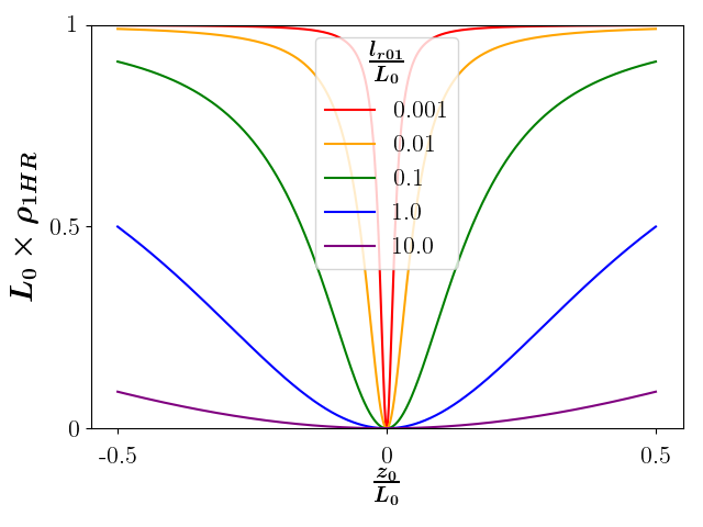
(a)

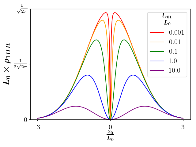
(b)

Figure 1: Shape of the planar symmetric asymptotic density for (a.) uniform and (b.) Gaussian initial distributions. $L_{0}$ represents the initial width of the distribution, $l_{r01}=\frac{\epsilon_{0}mc^{2}}{q\Sigma_{tot}}$ is the length scale associated with the density of the particles, and $\Sigma_{tot}$ is the charge per unit area of the distribution as described in the text. Notice that these graphs are independent of the exact choices of $L_{0}$. Further notice the quadratic like behavior in the middle as well as at large values of $\frac{l_{r01}}{L_{0}}$ for the uniform distribution. Finally note the fact that the distribution approaches the original distribution at its maximum value when $\frac{l_{r01}}{L_{0}}$ is small. What is not displayed is that the maximum peak is proportional to $\frac{1}{l_{r01}}$ when $\frac{l_{r01}}{L_{0}}$ is large.

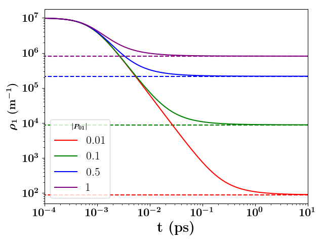
(a) uniform

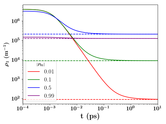
(b) Gaussian

Figure 2: Theoretical density evolution (solid lines) of specific distribution points in the free expansion of the bunch demonstrating the origin of the relativistic shock. The dotted lines indicate the asymptotic value determined by Eq. (45). The points correspond to locations that symmetrically contain approximately 1%, 10%, 50%, and either 100% (uniform) or 99% (Gaussian) of the distribution as indicated by their $P_{01}$ value. The time scales of all points inversely correlate with their location in the distribution (see Eq. (42)). For the uniform distribution (a), all points start at the same density but converge to different asymptotes according to the inverse relationship between position and time scale. This leads to a parabolic distribution as seen in Eq. (47) as $L_{0}<<l_{r01}$ here. For the Gaussian distribution (b), the fact that the outer points have lower initial densities leads to density trajectories crossing indicating the formation of the density peak that goes both up and down in contrast to the sharp peak seen in the uniform case.

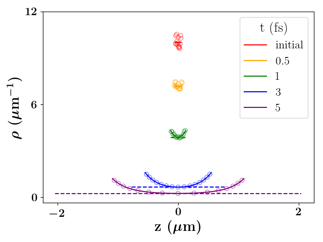
(a)

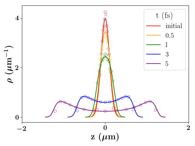
(b)

Figure 3: Theoretical predictions (solid line) and $M$-shell simulations (hollow dots) of the density at 4 different times with different initial conditions. Notice the offset of the $0$ value on the y-axis. The simulation had either (a) $L=0.1~{}\mu$m or (b) $\sigma_{L}=0.1~{}\mu$m, $\Sigma_{tot}=10^{8}$ electrons per $\mu$m², and $M=10,000$. The extremely high density was chosen as this density does not require significant expansion of the bunch before the onset of relativistic effects. The dotted lines in (a.) represents the non-relativistic prediction of the uniform distribution, and the purple dotted line extends beyond the ends of the $x$-axis but are not shown to keep the scale of expansion closer to what is seen relativistically; notice that the dotted line is tangent to the relativistic distribution at the same time at $r=0$. The deviation of the theory above the dotted line and toward the center of the bunch indicates density freezing due to electrons obtaining luminal speeds whereas the non-relativistic particles become super-luminal. Simulations were accomplished by randomly sampling $M$ macro-particles and advancing them according to the relativistic position equations derived in the text.

The mechanism for the relativistic peak emergence may be further seen in Fig. 2 where the density associated with different Lagrangian particles within the distribution are tracked and shown to asymptote to various density values predicted by Eq. (45). One way to describe this mechanism is to notice that all particles, excepting the center particle, in a planar model will asymptote to the speed of light. As the density is physically smooth, the particles’ velocities in the neighborhood of the Lagrangian particle asymptote similarly to the speed of light. In other words, the relative velocity of the particles in the Lagrangian particle’s neighborhood asymptotes to zero, and the particles cease to spread in the $z$ dimension. As the $z$ dimension is the only dimension in which the density is spreading in the planar model, this is the same as freezing the density to a constant value – an asymptote. Moreover, as particles toward the edge of the distribution have larger accelerations, these particles asymptote earlier than particles farther in. These differences in “freezing” time result in the middle of the distribution expanding, and becoming less dense, before the onset of the relativistic regime. Coupled with the initial distribution, this results in the formation of density peaks toward the edge of the distribution, as is seen in both the uniform and Gaussian distributions in Fig. 3. In the non-relativistic limit, there is no Coulomb shock in planar bunches with cold initial conditions; while in the relativistic limit a strong shock emerges and an initial bunch described by either uniform or a Gaussian density distribution evolves to a two peak structure with one bunch moving to the right and the other to the left (see Fig. 3).

Also apparent in Fig. 3 is the fact that stochastic effects are initially strong in simulated density profiles. However, at long times the theoretical density and simulated density agree well. This is a real effect. Specifically, consider the inter-particle distance between the $i^{th}$ and $(i+1)^{th}$ shells denoted as $d_{i}$. For a uniform distribution, order statistics tells us that $d_{i}(0)=\frac{L}{M+1}+\epsilon$ where $L$ is the total width of the distribution, $M$ is the total number of shells, and $\epsilon$ is a stochastic factor roughly of the size $\frac{L}{M+1}$. Thus, due to stochastic fluctuations, we’d expect some sheets to be bunched together giving a higher local density than the average and likewise other sheets to be further apart giving a lower local density than the average. This is precisely what is seen with the initial distribution in Fig. 3. However, as these sheets evolve, the relative non-relativistic acceleration is $\frac{2qE_{T1}}{mM}$, so $d_{i}(t)=d_{i}(0)+\frac{qE_{T1}}{mM}t^{2}$. Given sufficient time, $t>>\sqrt{\frac{mL}{qE_{T1}}}$, $d_{i}(t)\approx\frac{qE_{T1}}{mM}t^{2}$. That is, the inter-particle distance (and hence the distribution) is dominated by the space-charge effect and converges to the space-charge predicted distribution everywhere. Of course, if the bunch enters the relativistic regime prior to this smoothing, the stochastic effects will be preserved. We will see such behavior once we add an extraction field, but such behavior requires extremely dense bunches that may not be physically possible in free expansion experiments.

II.3 Cylindrical symmetry

Now we consider the expansion of an initially cold charged particle cloud with cylindrical symmetry. In this case, Eq. (20) becomes

$$v =\frac{\sqrt{2}\zeta y\sqrt{1+\zeta^{2}y^{2}}}{1+2\zeta^{2}y^{2}}c$$ (48)

where $y^{2}=\ln\left(\frac{r}{r_{0}}\right)$, $\zeta^{2}=\frac{r_{0}\rho_{r02}}{2}=\frac{r_{0}P_{02}}{2l_{r02}}=\frac{r_{0}^{2}\omega_{02}^{2}}{4c^{2}}$, with $\rho_{r02}$ coming from Eq. (33). As $l_{r02}\propto r_{0}$, it should be apparent that $\zeta$’s dependence on $r_{0}$ is completed determined by $P_{02}(r_{0})$.

From Eq. (48) and (21), we find the implicit relation between time and radial position through the integral,

$$t =\frac{2}{\omega_{02}}\int_{0}^{\sqrt{\ln\left(\frac{\tilde{r}}{r_{0}}\right)}}\frac{1+2\zeta^{2}y^{2}}{\sqrt{1+\zeta^{2}y^{2}}}e^{y^{2}}dy.$$ (49)

To make the connection with previous work, we introduce a generalized Dawson function $\mathcal{F}$ through the definition,

$$\mathcal{F}(g,x)=e^{-x^{2}}\int_{0}^{x}g(\zeta,z)~{}e^{z^{2}}dz$$ (50)

where $\zeta$ can be written as a function of $x$. Thus the time-spatial relation may be expressed as

$$t =\frac{2}{\omega_{02}}\frac{r}{r_{0}}\mathcal{F}\left(g(\zeta,y),y\right)$$ (51)

where

$$g(\zeta,y)=\frac{1+2\zeta^{2}y^{2}}{\sqrt{1+\zeta^{2}y^{2}}}$$ (52)

When $g(\zeta,y)=1$, we reproduce the Dawson function, $F(x)=\mathcal{F}(1,x)$. Specifically when we are in the non-relativistic regime, we have $2\zeta y<<1$ and $g(\zeta,y)\approx 1$, so Eq. (51) reduces to

$$t \approx\frac{2}{\omega_{02}}\frac{r}{r_{0}}F(y)$$ (53)

which is the result we derived previously in the non-relativistic case. We can write down the derivative of the generalized Dawson function by applying the Leibniz rule

$$\frac{d\mathcal{F}}{dx} =-2x\mathcal{F}(g,x)+g(\zeta,x)+\mathcal{F}\left(\frac{\partial g}{\partial\zeta},x\right)\frac{d\zeta}{dx}$$ (54)

Note that in the non-relativistic limit, $g(\zeta,y)=1$, and Eq. (54) reduces to the normal Dawson function derivative $\frac{dF}{dx}=-2xF(x)+1$.

Following the same reasoning as our previous workZerbe et al. (2018), we can obtain an analytic form for the time dependent density, i.e. the density evolution expression (see Eq. (25)). Evaluating $r^{\prime}=\frac{dr}{dr_{0}}$ by taking a derivative of Eq. (51) with respect to $r_{0}$, we find,

$$r^{\prime} =\frac{r}{r_{0}}\left(1+\frac{2y}{g(\zeta,y)}\left(D_{02}\ \mathcal{F}-\frac{\rho_{02}}{{\bar{\rho}}_{02}}\zeta\mathcal{F}_{\partial}\right)\right)$$ (55)

where $\mathcal{F}$ is shorthand for $\mathcal{F}(g(\zeta,y),y)$ $\mathcal{F}_{\partial}$ is shorthand for $\mathcal{F}\left(\frac{\partial g}{\partial\zeta},y\right)$, and $D_{02}$ is from Eq. (2). Note $D_{02}$ measures the deviation from a uniform cylindrically-symmetric distribution, and for the uniform cylindrically-symmetric distribution case it is zero for all values of $r_{0}$ where $\rho_{0}$ is not $0$.

From the above analysis, the density evolution is found to be,

$$\rho_{2}(r;t) =\frac{r_{0}^{2}}{r^{2}}\frac{\rho_{02}}{1+\frac{2y}{g(\zeta,y)}\left(D_{02}\ \mathcal{F}-\frac{\rho_{02}}{{\bar{\rho}}_{02}}\zeta\mathcal{F}_{\partial}\right)}$$ (56)

In Fig. 4, we compare the predictions of Eq. (56) to simulations for both uniform and Gaussian initial distributions. We choose the initial radius and radial standard deviation, respectively, to be 1 cm for $N=1\times 10^{13}$ electrons/cm. We again simulate with Warp using the EM solver as well as the 2D version of $M$-shell simulations. For the $M$-shell simulations, the initial radius of the $M$ cylindrical shells are sampled and then evolved according to Eq. (48) and Eq. (53) but with $\omega_{02}$ replaced by $\sqrt{\frac{3q\Lambda_{s}}{\pi r_{s,0}^{2}m\epsilon_{0}}}$ where $\Lambda_{s}$ is the charge per unit length contained in the cylindrical shell and $r_{s,0}$ is the initial radius of the shell. As can be seen in Fig. 4, the theory and both simulations agree on the evolution of both the uniform and non-uniform initial distributions. Similar to the planar case, the initial variance about the predicted value can be seen to decrease as the simulations evolve. Again, this indicates that the inter-shell distances are dominated by the space-charge effects resulting in the later simulations having less statistical variation from the expected distribution.

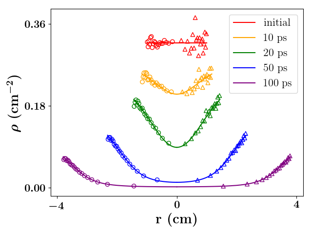
(a)

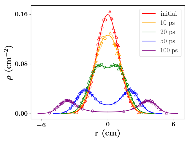
(b)

Figure 4: Theoretical predictions (solid line), cylindrical $M$-shell simulations (hollow triangles–right), and PIC simulations using an EM solver (hollow circles–left) of the density at 5 different times for the cylindrically symmetric case. PIC simulations were analyzed using the middle 2m from a simulation of a 20m-long, 3D distribution of electrons with periodic boundary conditions on the z-axis. The theory prediction is reflected about the origin as $r$ is strictly greater than 0 and the simulations are separated into the first and second quadrant for purposes of visualization. Parameters were $N=1\times 10^{13}$ electrons/cm, $R_{0}=\sigma_{r,0}=1~{}$cm, and $M=50,000$. Like the planar symmetric case, the density at the center continues to decrease non-relativistically indicating that the density above the density at the center is due to relativistic effects; however, notice that this peak continues to decrease instead of the evolution freezing at luminal speeds as seen in the planar symmetric case.

In the non-relativistic regime, $2\zeta y<<1$; $\mathcal{F}\to F$ and $\zeta\mathcal{F}_{\partial}\to 0$. Thus Eq. (56) reduces to

$$\rho_{2}(r;t) =\frac{r_{0}^{2}}{r^{2}}\frac{\rho_{02}}{1+2D_{02}\ yF(y)}$$ (57)

which is the expression we found in our earlier, non-relativistic workZerbe et al. (2018).

Similar to the planar symmetric case, we are interested in the density the distribution should evolve under specific limits. We were unable to analytically obtain a limit analogous to the limit we found under planar symmetry in Eq. (45) as doing so requires evaluating the value of the modified Dawson function as $\ln\left(\frac{r}{r_{0}}\right)$ goes to infinity. We were able to see the freezing of the dimension in the extremely dense limit where $\zeta>>1$ as we have shown in Appendix C . Specifically, the evolution at the edge of the distribution can be approximated by $\rho_{2}(r;t)=\frac{r_{0}}{r}\rho_{0}$, which is the evolution of the uniform distribution under non-relativistic conditions in one-dimension lower, i.e. 1D. This situation is analogous to the high density 1D case that causes the edges to essentially immediately become relativistic likewise resulting in evolution of the uniform distribution under non-relativistic conditions in one-dimension lower, i.e. 0D or constant. However, this condition, $\zeta>>1$, is analogous to the 1D case when the entire distribution is essentially in the highly relativistic limit. We will shortly show that even in this case, the spherically symmetric evolution can be shown to freeze out a dimension; however, we believe that this freezing happens for cylindrically symmetric distributions regardless of the size of $\zeta$.

II.4 Spherical symmetry

Now we consider the expansion of an initially cold charged particle cloud with spherical symmetry. In this case, Eq. (20) becomes

$$v =2\zeta x\frac{\sqrt{g_{1}(x)}}{g_{2}(x)}c$$ (58)

where $x^{2}=1-\frac{r_{0}}{r}$, $g_{1}(x)=1+\zeta^{2}x^{2}$, $g_{2}(x)=1+2\zeta^{2}x^{2}$, $\zeta^{2}=\frac{r_{0}\rho_{r03}}{2}=\frac{r_{0}P_{03}}{2l_{r03}}=\frac{r_{0}^{2}\omega_{03}^{2}}{6c^{2}}$, and $\rho_{r03}$ is from Eq. (33). As $l_{r03}\propto r_{0}^{2}$, it should be apparent that $\zeta\propto r_{0}P_{03}(r_{0})$.

From Eq. (48) and (21), we find the implicit relation between time and radial position through the integral,

$$t =\frac{\sqrt{3/2}}{g_{1}(1)\omega_{03}}\left(g_{2}(1)\frac{r}{r_{0}}x\sqrt{g_{1}(x)}+T(x)\right)$$ (59)

where $T(x)=\tanh^{-1}\left(\sqrt{\frac{g_{1}(1)}{g_{1}(x)}}x\right)$. Note that the $1$ inside the $g$ functions corresponds to $x$ at infinitely long times, i.e. $\lim_{\frac{r}{r_{0}}\to\infty}x=1$, so $g_{1}(1)=1+\zeta^{2}$ and $g_{2}(1)=1+2\zeta^{2}$. This expression is essentially the same expression as derived by Bychenkov and Kovalev, who first derived it for the case of uniform initial density distributions Bychenkov and Kovalev (2011). Our expression differs only in the interpretation of $\omega_{03}$ as ours can be dependent on $r_{0}$ whereas their $\omega_{03}$ is a constant, which is the correct interpretation for the uniform distribution. This difference in interpretation allows us to treat general initial distributions but requires additional consideration when determining the derivative of Eq. (59) with respect to $r_{0}$ as $\omega_{03}^{\prime}=\frac{3\omega_{03}}{2r_{0}}D_{03}$, where ${}^{\prime}\equiv\frac{d}{dr_{0}}$, with the $d$’s in this last expression representing differentiation – not dimensionality of the problem, and $D_{03}$ is from Eq. (2).

We follow the same reasoning as our previous work Zerbe et al. (2018) in order to obtain the density evolution expression. After taking the derivative of Eq. (59) with respect to $r_{0}$, we can solve for $r^{\prime}$ giving

$$r^{\prime} =\frac{r}{r_{0}}\frac{1}{(g_{1}(1))^{2}g_{2}(x)}\left(p_{1}(x)+\frac{r_{0}}{r}p_{2}(x)T(x)\right)$$ (60)

where

$$p_{1}(x) =g_{1}(1)+\frac{3}{2}D_{03}x^{2}g_{1}(x)+3\zeta^{4}D_{03}x^{2}\frac{r_{0}}{r}$$ (61)

and

$$p_{2}(x) =\left(3\zeta^{2}+6\zeta^{2}D_{03}+\frac{3}{2}D_{03}\right)x\sqrt{\frac{g_{1}(x)}{g_{1}(1)}}$$ (62)

Plugging Eq. (60) into Eq. (25) we obtain the evolution of the density distribution

$$\rho_{3}(r;t)=\frac{r_{0}^{3}}{r^{3}}\frac{(g_{1}(1))^{2}g_{2}(x)\rho_{0}}{p_{1}(x)+\frac{r_{0}}{r}p_{2}(x)T(x)}$$ (63)

In Fig. 5, we compare the prediction of Eq. (63) to simulations for both a uniform and Gaussian initial distributions of $N=1\times 10^{13}$ electrons. The simulation have $R=1$ cm (uniform) or $\sigma_{r}=1$ cm (Gaussian). We again simulate with Warp using the EM solver and as well as the 3D version of $M$-shell simulations. For the $M$-shell simulations, the initial radius of the $M$ spherical shells are sampled and then evolved according to Eq. (58) and Eq. (59) but with $\omega_{03}$ replaced by $\sqrt{\frac{3qQ_{s}}{4\pi r_{s,0}^{3}m\epsilon_{0}}}$ where $Q_{s}$ is the charge contained in the shell and $r_{s,0}$ is the initial sampled radius of the shell. As can be seen in Fig. 5, the theory captures the evolution of both the uniform and non-uniform initial distributions. Similar to both the planar and cylindrical cases, the initial variance around the theoretical value primarily seen in the uniform distribution decreases as the distribution expands.

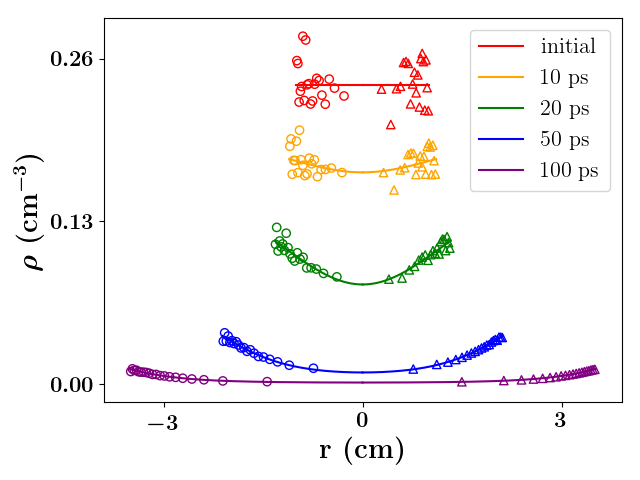
(a)

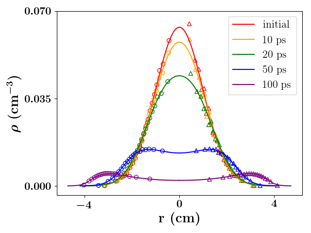
(b)

Figure 5: Theoretical predictions (solid line), spherical $M$-shell simulations (hollow triangles–right), and PIC simulations using an EM solver (hollow circles–left) of the density at 5 different times for the spherically symmetric case. The theory is reflected about the origin as $r$ is strictly greater than 0 and the simulations are separated into the first and second quadrant for purposes of visualization. Parameters were $N=1\times 10^{13}$ electrons, $R_{0}=\sigma_{r,0}=1~{}$cm, and $M=5000$. Like the planar and cylindrical symmetric cases, the density at the center continues to decrease non-relativistically indicating that the density above the density at the center is due to relativistic effects; similar to the cylindrical symmetric case, the relativistic density continues to evolve. However, the evolution of the peak decreases much faster than the cylindrical case — which is discussed in detail in the text.

For further validation, we compare Eq. (63) to the expression derived by Bychenkov and Kovalev. Their expression detailed the relativistic density evolution for the uniform distributionBychenkov and Kovalev (2011), $\rho_{unif}(r;t)$, which should be equivalent to our expression when $D_{03}=0$. In this case, Eq. (63) reduces to

$$\rho_{3unif}(r;t) =\frac{r_{0}^{3}}{r^{3}}\frac{(g_{1}(1))^{2}g_{2}(x)\rho_{0}}{g_{1}(1)+\frac{r_{0}}{r}3\zeta^{2}x\sqrt{\frac{g_{1}(x)}{g_{1}(1)}}T(x)}$$ (64)

This expression for the density evolution for uniform initial conditions is identical to the expression published in the English translation of Bychenkov and Kovalev except for an obvious typo in that workBychenkov and Kovalev (2011).

Next, we compare this expression to our previous, non-relativistic expression. In the non-relativistic regime $2\zeta^{2}<<1$. Unlike the planar and cylindrical cases, the spherical model need never enter the relativistic regime and therefore this model may be relevant for all time. In this non-relativistic regime, Eq. (63) reduces to

$$\rho_{3NR}(r;t) =\frac{r_{0}^{3}}{r^{3}}\frac{\rho_{0}}{1+\frac{3}{2}D_{03}\left(x^{2}+\frac{r_{0}}{r}x\tanh^{-1}x\right)}$$ (65)

which is identical to the non-relativistic expression we previously derived but with $D_{03}=D$ in our previous notationZerbe et al. (2018).

Again we would like to analyze specific limits of the density evolution; fortunately, under spherical symmetry we can analyze the long time limit. In Appendix B we show that

$$\lim_{\frac{r}{r_{0}}\to\infty}\rho_{3} =\frac{r_{0}^{3}}{r^{3}}\rho_{x3}(r_{0})$$ (66)

where $\rho_{x3}(r_{0})=\frac{1+3\zeta^{2}+2\zeta^{4}}{1+\frac{3}{2}D_{03}}\rho_{03}$ is entirely determined by the initial conditions. Notice, the pre-factor in $\frac{1+3\zeta^{2}+2\zeta^{4}}{1+\frac{3}{2}D_{03}}$ is essentially $1$ in the center where $\zeta\approx 0$ and $D_{03}\approx 0$, but that this value increases as $r_{0}$ increases. The time evolution of $\rho_{x3}$ and the predicted asymptote for this quantity can be seen in Fig. 6. For the uniform distribution, the increase in $\rho_{x3}$ as a function of $r_{0}$ is quartic as $D_{03}=0$ for all values of $r_{0}$. In real distributions, though, there should be a value for $r_{0}$ where $D_{03}=-\frac{2}{3}$, and we see that $\rho_{x3}$ has a zero in the denominator. This violates the assumptions made in the derivation of $\rho_{x3}$, and inspection of Appendix B shows that $r^{\prime}$ becomes $0$ in the locality of $D_{03}=-\frac{2}{3}$ suggesting a violation of the laminar fluid assumption. For the Gaussian distribution, roughly 80% of the distribution is contained within the radius where $D_{03}(r_{0})=-\frac{2}{3}$ suggesting that at least the majority of the distribution is captured by this theory. Furthermore, the the precise shape for $\rho_{x3}(r_{0})$ for a uniform and Gaussian distribution may be seen in Fig. 7; however, in the 1D case, $\rho_{01}$ truly asymptotes whereas here $\rho_{03}$ continues to decrease eventually with the uniform-like behavior of $\frac{r_{0}^{3}}{r^{3}}$. This difference is largely due to the fact that all particles asymptote to the same velocity, $c$, in the planar case but different velocities in the spherical case.

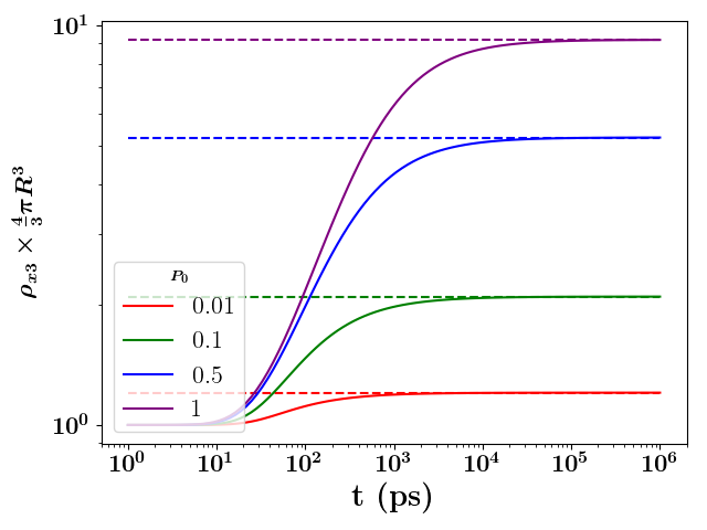
(a)

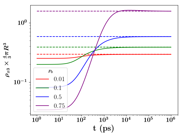
(b)

Figure 6: The time evolution (solid lines) of $\rho_{x3}$, defined in the text, for a distribution with $1.602mC$ in (a) an initially uniform sphere of width 1 mm and (b) an initially Gaussian sphere with standard deviation of 1mm. The dashed lines indicate the corresponding highly-relativistic limit of $\rho_{x3}$ obtained analytically. Again, the formation of the density peak from these relativistic considerations is apparent in the graphs. Similar to how the planar symmetric density freezes, $\rho_{x3}$ can be seen to asymptote; however, this is due to the Lagrangian particle reaching their terminal velocity, the difference of which is relativistically contracted, as described in the text.

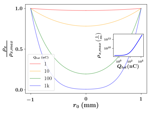
(a)

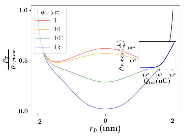
(b)

Figure 7: The shape of $\frac{\rho_{x3}}{\rho_{x3,max}}$ for various values of $Q_{tot}$ in (a) an initially uniform distribution with radius of 1 mm and (b) an initially Gaussian distribution with standard deviation of 1 mm as a function of the initial radial coordinate. This, as well as the inset figure describing the growth of the maximum value of $\rho_{x3}$, show the onset of the relativistic regime corresponding to roughly $24\frac{C}{m}$. The main graph also shows that the peaks sharpen as the density increases. For the Gaussian case, this distribution diverges near $r_{0}=2$. This divergence is an indication that the laminar fluid assumption is being violated, and therefore the non-uniform asymptote for $\rho_{x3}$ should be taken as a gross approximation; nonetheless, the expression derived in the text do capture the shape of freely-expanding relativistic Gaussian distribution in the simulation presented in Fig. 5. L

This analysis leads to the second limit of $\lim_{\zeta\to\infty}$, an unphysical limit, analogous to the 1D and cylindrically-symmetric cases where we saw the density at the edge lose dimensionality. Likewise, in the spherical-symmetric case we show in Appendix C that

$$\lim_{\zeta\to\infty}\rho_{3}(r;t)=\frac{r_{0}^{2}}{r^{2}}\rho_{03}$$ (67)

which is again the uniform density evolution of a symmetric distribution in one dimension less than the one being considered. While appearing unphysical, this does have some physical significance, though. This suggests that such distribution evolve toward $\rho_{x}(r_{0})$ in such a way that the factor in the denominator exactly cancels out the factor of $\frac{r_{0}}{r}$, i.e. $r^{\prime}\approx 1$ early on. However, as time progresses, the evolution shifts toward the decay of the uniform distribution in the appropriate dimension.

III Extraction field in the planar model

It is straightforward to introduce an extraction field in the planar model, and this is relevant to dynamics of electron density distributions in the pancake bunches used in ultrafast electron microscopy. The equations for this case are identical to the equations derived for the planar model in the absence of an extraction field with the single replacement

$$P_{01} \rightarrow P_{01}+\frac{E_{a}}{E_{T1}}$$ (68)

or equivalently

$$\rho_{r01} \rightarrow\rho_{r01}+\rho_{a}$$ (69)

where $\rho_{r01}$ is from Eq. (33) and $\rho_{a}=\frac{eE_{a}}{mc^{2}}$, which also can be interpreted as a new length scale, $l_{a}=\frac{mc^{2}}{eE_{a}}$, associated with the extraction field. We choose the applied field to be in the positive $z$ direction. For applied fields, $E_{a}$, with $E_{a}>E_{T1}$ ($l_{a}<l_{r01}$) the applied field is sufficiently strong to overcome the space charge field throughout the bunch, hence accelerating all of the particles in the same direction. For smaller applied fields, $E_{a}<E_{T1}$ ($l_{a}>l_{r01}$), particles in the negative $z$ regions of the initial charge distribution may experience a stronger intrinsic space charge field than can be overcome by the applied field. In this case the initial distribution breaks up into two bunches moving in opposite directions. This is the virtual cathode limit defined by Valfells et al.Valfells et al. (2002). We also point out that $l_{r01}$ corresponds to the length scale of this limit. The fraction of charge in the bunch that moves in the positive and negative $z$ direction is simply $\frac{1}{2}\left(1\pm\frac{E_{a}}{E_{T1}}\right)$, respectively . The form of the two bunches is given by Eq.(40), with the substitution given in Eq. (68). Taking the relativistic limit of this expression, we obtain the asymptotic form of the two bunches

$$\rho_{1HR}(z;t) \rightarrow\frac{\rho_{01}}{\frac{1}{l_{r01}}\left(P_{01}+\frac{E_{a}}{E_{T1}}\right)^{2}+\rho_{01}}\left(P_{01}+\frac{E_{a}}{E_{T1}}\right)^{2}$$ (70)

and the asymptotic form for the uniform and Gaussian distributions for various applied fields are demonstrated in Fig. 8. Eq. (70) can be written in terms of the plasma period, $\omega_{01}$, and other terms, but we find that both the applied field scale, $E_{T1}$, and the associated length scale, $l_{r01}$, are more apparent in this formulation.

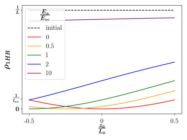
(a) uniform

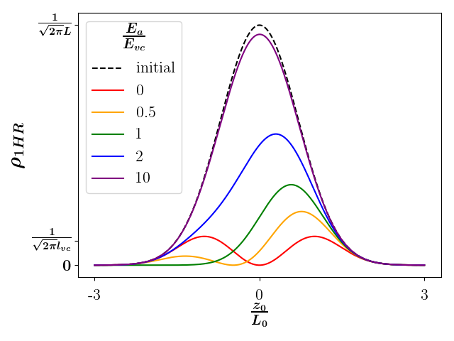
(b) Gaussian

Figure 8: Theoretical planar symmetric asymptotic distributions (solid lines) plotted against the initial position for various applied fields, measured in multiples of $E_{T1}=\frac{\Sigma_{tot}}{2\epsilon}$. The black dotted line indicates the initial distribution. Notice that in both cases, the actual distribution is located at $z(t)$ at time $t$, but as this has a one-to-one relation with $z_{0}$, we use the initial location for the sake of comparison.

For the case of a uniform initial distribution $\rho_{01}=\frac{1}{2L}$ on the domain $[-L,L]$, the field of a particle at position $z_{0}$ is given by

$$E_{01}(z_{0})+E_{a}=E_{T1}\frac{z_{0}}{L}+E_{a}$$ (71)

Setting the total field to zero gives the point at which the pulse breaks up into two pulses,

$$z_{x}=-\frac{E_{a}}{E_{T1}}L$$ (72)

Notice that as $E_{a}$ goes above $E_{T1}$, $z_{x}$ goes below $-L$ indicating that there is no split in the pulse consistent with prior analysis. As long as $E_{a}<E_{T1}$, the peak density of each pulse after it has gone relativistic can be calculated from Eq. (70) and is

$$\rho_{1right/left} =\frac{1}{2L+l_{r01}\left(\frac{E_{a}}{E_{T1}}\pm 1\right)^{-2}}$$

again with the positive, rightward pulse corresponding to the $+$ and the negative, leftward pulse corresponding to the $-$.

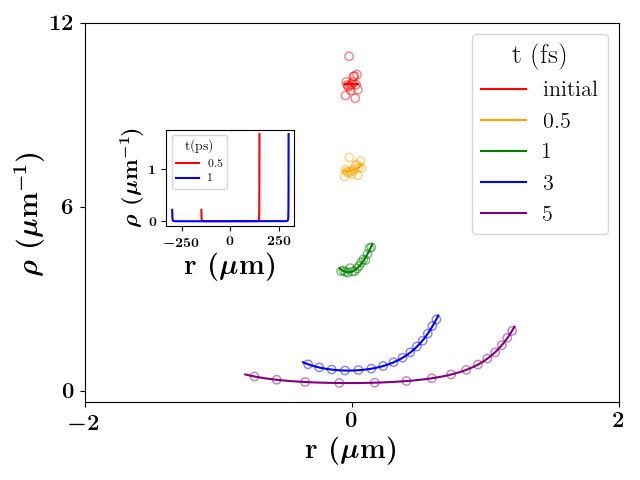
(a) $E_{a}=0.5~{}E_{T1}$

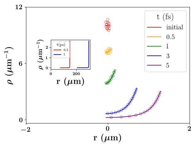
(b) $E_{a}=E_{T1}$

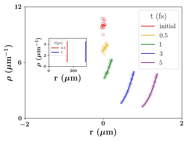
(c) $E_{a}=2~{}E_{T1}$

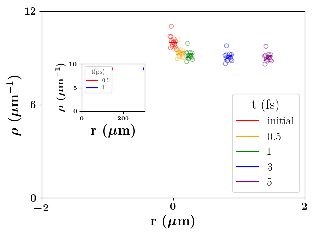
(d) $E_{a}=10~{}E_{T1}$

Figure 9: Theoretical predictions (solid line) and $M$-shell simulations (hollow dots) of the planar symmetric density at 4 different times with different applied extraction fields. The simulation had $L=0.1~{}\mu$m and $\Sigma_{tot}=1\times 10^{20}$ electrons per m² and $M=10,000$. The extremely high density was chosen as this density not require significant expansion of the bunch before the onset of relativistic effect. Simulations were similar to those described in Fig. 3, and again the inset graphs show the theoretic density at 2 much later times (0.5 and 1 ps). While the distributions at later times appear delta-like, they do have at least the same width as seen at earlier time — however, this width is much smaller than the scale resulting in the delta-like behavior at later times. Notice that in the main plot the scales are consistent among graphs. Also notice that the extraction fields have little effect on where the front of the bunches are after 1 ps but have dramatic effect on the bunch distribution — this is partially an artifact of the high density of the initial distribution that results in the front of the distribution relatively quickly becoming relativistic with or without an extraction field. In addition to the shape of the asymptotic density, the extraction field determines to what extent the initial variance about the mean-field theory prediction is lost (an effect explained in the text.)

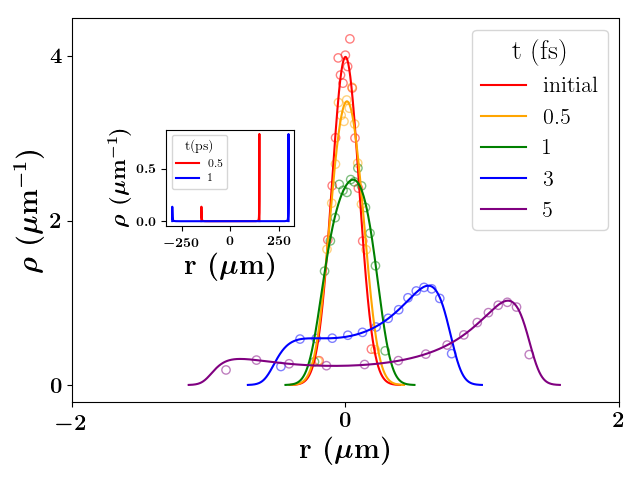
(a) $E_{a}=0.5~{}E_{T1}$

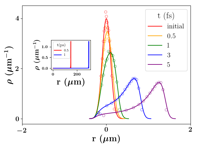
(b) $E_{a}=E_{T1}$

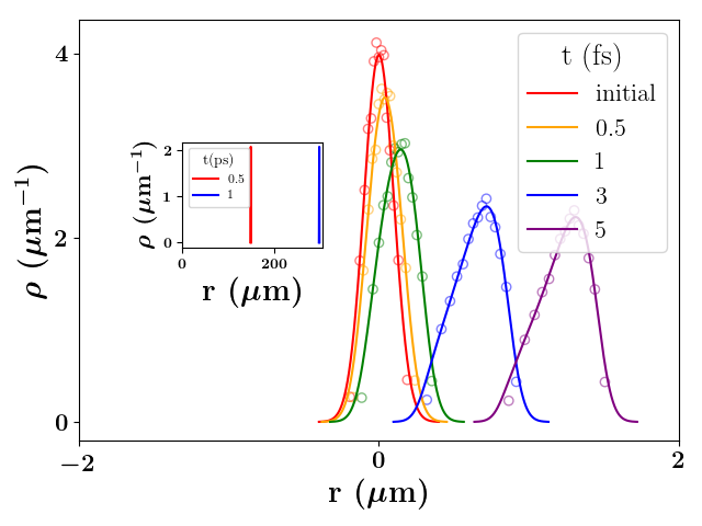
(c) $E_{a}=2~{}E_{T1}$

(d) $E_{a}=10~{}E_{T1}$

Figure 10: Theoretical predictions (solid line) and $M$-shell simulations (hollow dots) of the planar symmetric density at 4 different times with different applied extraction fields. Parameters and simulations are analogous to those described in Fig. 9 excepting the initial Gaussian distribution with $\sigma_{r}=0.1~{}\mu$m.

The effect of the extraction field on the time-dependent density evolution can be seen in Figs. (9) and (10), which show the evolution of initially uniform and Gaussian distributions, respectively, in the presence of various extraction fields. First, notice that the inclusion of a non-zero $E_{a}$ breaks the symmetry of the left and right pulses and that we can see that the double pulses are replaced by a single pulse as the applied field crosses the virtual cathode limit, $E_{a}=E_{T1}$. As $E_{a}$ is increased beyond $E_{T1}$, all Lagrangian particles eventually become relativistic, and the density “lifts” away from the axis. Eventually (not shown), the extraction field should be strong enough that no appreciable expansion occurs and the initial distribution is simply displaced at the speed of light; this can be shown to occur when $E_{a}>>E_{T1}$.

Also as can be seen in Figs. (9) and (10), the initial stochastic variation in the density is lost for simulations of sufficiently low extraction field but is retained for $E_{a}\geq 10E_{T1}$. This is due to the same effect discussed in the planar model without an electric field; however, the relativistic time scale needs to be adjusted, namely

$$\tau_{rel}=\frac{l_{r01}}{c}\left|P_{01}+\frac{E_{a}}{E_{T1}}\right|^{-1}$$ (73)

When $\tau_{rel}>>\tau_{exp}$, we again have the case where the expansion dynamics dominate and the inter-particle spacings essentially are equivalent to the inter-particle spacings determined by theory. However, once $\tau_{rel}<<\tau_{exp}$, the inter-particle spaces do not expand sufficiently to overcome the initial stochastics and the variance is preserved. The new wrinkle is that $\tau_{rel}$ can be reduced by simply increasing the extraction field. Therefore, we do in fact see a distribution evolve that retains the initial variance, i.e. $E_{a}=10E_{T1}$ in Fig. 9, as for that simulation $\tau_{rel}<<\tau_{exp}$.

Moreover, the influence of the extraction field is important in the highly relativistic regime not only for influencing the time scale but also influencing the asymptotic distribution. Specifically, the effect of the extraction field in the 1D model is apparently not to accelerate the front of the distribution, i.e. all simulation had the front of the bunch traveling near the speed of light, but instead to shape the eventual distribution as can be seen in Figs. (9) and (10). The asymptotic densities for the initially uniform and Gaussian distributions and for various extraction fields can be seen in Fig. 8 where we have used Eq. (45). Specifically, every point besides the point corresponding to $P_{01}+\frac{E_{a}}{E_{T1}}=0$ will eventually have $|P_{01}+\frac{E_{a}}{E_{T1}}|\frac{ct}{l_{r01}}>>1$ and thus the density corresponding to such points will eventually become a constant. However, while $|P_{01}+\frac{E_{a}}{E_{T1}}|\frac{ct}{l_{r01}}$ is not much larger than $1$, the density of the point will decrease toward the eventual constant value.

IV Application of the 1D distribution

In this section, we demonstrate one use of the spatial distributions; specifically, we calculate the width evolution of UEM-relevant planar-symmetric distributions as a function of time. Specifically, we define the rms width of the distribution as

$$\sigma_{z} =\sqrt{<z^{2}>-<z>^{2}}$$ (74)

Theoretically $<a>=\int_{-\infty}^{\infty}a\rho_{1}dz=\int_{-\infty}^{\infty}a(z_{0})\rho_{01}dz_{0}$, and in simulation $<a>=\frac{1}{N}\sum_{i=1}^{N}a_{i}$ where $N$ is the number of particles in the simulation and $a_{i}$ is the value of $a$ for the $i^{th}$ particle.

We consider a Gaussian bunch with transverse radius of $100~{}\mu$m and longitudinal width of $\sigma_{r}=0.1~{}\mu$m, and we consider both $N=10^{6}$, relevant for diffraction studies, and $N=10^{8}$, relevant for imaging studies. We treat the longitudinal expansion with the planar model both using the non-relativistic distribution, Eq. (43), as well as the relativistic version, Eqs. (40) and (69). We calculate the theoretical expectation numerically for initially Gaussian distributed planar-symmetric distributions for various values of $E_{a}$ as well as the non-relativistic width prediction and compare the results to the standard deviation of $M=10^{4}$-shell simulations with the same parameters. Results of this treatment may be seen in Fig. 11.

As can be seen in Fig. 11, the theory and simulations result in the same width evolution. It is worth noting that $E_{T1}\approx 0.3MV/m$ for $N=10^{6}$ and $E_{T1}\approx 30MV/m$ for $N=10^{8}$. As can be seen in the figures, the width growth does not vary much from the unaccelerated case until an extraction field is increased beyond $\approx 10~{}E_{T1}$, that is the expansion dynamics will dominate the width determination until we are far beyond the “total” field within this 400 ps time frame. Also apparent is that, within this time frame, the dynamics of the un-accelerated bunch does not differ from the non-relativistic model; on the other hand, the higher density dynamics do differ suggesting that relativistic expansion occurs in the $N=10^{8}$ planar model. Of course, as this bunch expands its longitudinal length will quickly become larger than the transverse width suggesting higher-dimensional dynamics will become important. Specifically after the transition to higher-dimensional dynamics, the planar model overestimates the longitudinal width and underestimates the transverse width. However, if a sufficient extraction field is obtained, i.e. around $100E_{T1}$, the asymptotic longitudinal width is of sufficiently small size to result in planar dynamics for the bunch meaning that the bunch width can be modeled with the planar model in that regime.

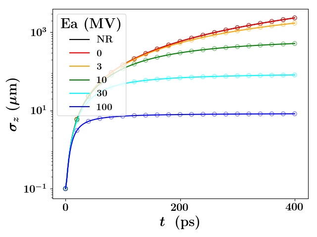
(a) $10^{6}~{}e$

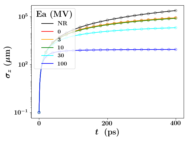
(b) $10^{8}~{}e$

Figure 11: Theoretical predictions (solid line) and $M$-shell simulations (hollow dots) of the width of an evolving planar-symmetric initially Gaussian distribution for two experiment relevant regimes. Both cases assumed a geometry of transverse width of $100~{}\mu$m and longitudinal width of $0.1~{}\mu$m, and they differed in the number of electrons in the bunch: (a) $10^{6}~{}e$ corresponding to an $E_{T1}\approx 0.3MV$ and (b) $10^{8}~{}e$ corresponding to an $E_{T1}\approx 3MV$. Notice that the y-axis is logarithmic, and the scales are different between the two plots. Also notice that relativistic effects of spreading of the bunch in the absence of an accelerating field within this time scale are not significant for the $10^{6}$ case but noticeable for the $10^{8}$ case. Furthermore, the accelerating field effect is noticeable within this time scale when $E_{a}=10MV$ for $10^{6}$ and $E_{a}=30MV$ for $10^{8}$; however, notice that in the $10^{8}$ case, the longitudinal beam width is larger than the transverse width and that the $1D$ model is probably no longer a valid approximation.

V Discussion and Conclusions

In this work, we extended our previous density evolution analysis into the relativistic regime. Specifically, we showed that the uniform distribution in any dimension develops density shocks as the outer portion of the distribution becomes relativistic; we also found expressions for such peaks in other distributions which occur in competition with the non-uniform Coulomb mechanism that leads to peaks in such distributionsZerbe et al. (2018). We showed that the analytic results accurately predicted 1D-like $M$-shell simulation results under all symmetries and PIC results under cylindrical and spherical symmetries. The PIC simulations conducted here were completed using an EM solver with an initial ES solve used to initialize the fields. As these simulations agree with the theory that is essentially based on electrostatics, it is apparent that EM effects beyond electrostatics are not significantly affecting the density evolution for the problems examined.

We emphasize that the mechanism for the relativistic shock development is distinct from non-relativistic shock development seen in the Gaussian distributionZerbe et al. (2018). Previously, we demonstrated that shocks arise in non-planar non-uniform distribution evolutions due to the initial distribution leading to non-linear Lagrangian particle velocities that lead to inner Lagrangian particles catching up to outer Lagrangian particles. On the other hand, shock in a relativistic bunch are caused by the “shrinking” of one-dimension of the density as the Lagrangian particles approach the luminal speed limit. This can be seen by considering the energy of continuum particles within the distribution. Specifically, as the particles expand, their kinetic energies increase according to Eq. (19). In the planar and cylindrically symmetric models, this increase is linear and logarithmic in their position (and eventually time), respectively, as can be seen by Eqs. (16) and (17). This leads to all particles in a neighborhood approaching the speed of light resulting in the “freezing” of the expansion along the expanding dimension; that is, all planar symmetric distributions eventually asymptote to a time independent density while all cylindrically symmetric distributions eventually expand “uniform-like” but with one dimension less than that being considered, i.e. $\rho_{2}\to\frac{r_{0}}{r}A\rho_{02}$ where $A$ is some parameter determined from the initial conditions. On the other hand, in the spherically symmetric case, the kinetic energy is bounded by $\frac{qQ_{tot}P_{03}}{4\pi\epsilon_{0}r_{0}}$, which is finite. As this kinetic energy is dependent on $r_{0}$ through $\frac{P_{03}(r_{0})}{r_{0}}$, the asymptotic velocity of neighboring continuum particles differs. This is why the density at long times for highly relativistic portions of the distribution drops in a uniform-like manner, i.e. $\rho_{3}\to\frac{r_{0}^{3}}{r^{3}}A\rho_{03}$ with $A=\frac{1+3\zeta^{2}+2\zeta^{4}}{1+\frac{3}{2}D_{03}}$ (see Eq. (66)). While both the planar and cylindrically symmetric cases lost a power to the uniform-like evolution, i.e. planar cases evolve like $\frac{1}{r^{0}}$ and cylindrically symmetric cases evolve like $\frac{1}{r^{1}}$, the spherically symmetric case’s uniform-like evolution retains $\frac{1}{r^{3}}$. This difference arises as the particles in the spherically symmetric case have finite potential energy and thus asymptote towards a velocity that is a little less than the speed of light. Now neighboring Lagrangian particles can have very small differences in their asymptotic velocity leading to the expansion in the radial direction being slower than what is seen non-relativistically; specifically, this is what leads to $A>1$. However, there does remain a non-vanishing small velocity difference meaning that the distribution continues to expand in all dimensions. Nonetheless, these effects lead to density peaks forming towards the edges of the distribution in all cases; regardless, we find it interesting that the behavior in each dimension is qualitatively unique.

Furthermore, we demonstrated that if the distribution is given enough time to expand, the stochastic effects in the initial distribution are overwhelmed by the space charge effects. This means that under such conditions, repeated instances of similar bunches should look more or less the same. However, if the bunch is quickly accelerated into the relativistic regime, the initial stochastic fluctuations are preserved.

While these results are somewhat surprising, we do need to emphasize that these conclusion are based on analyzing the symmetric models at long times and that some of the physical assumptions inherent in the models should be violated at some point. The three assumptions for these model are (1.) the temperature is small compared to the kinetic energy delivered to the particle due to Coulomb interaction, (2.) the distributions remain laminar, and (3.) the symmetry under consideration represents the physical situation. While these assumptions all break down to some extent at some point, we emphasize that in the simulations we have conducted that the model almost exactly matches with the PIC simulations.

Note that even as the distribution becomes more and more diffuse, if a region of the distribution had much less heat than the kinetic energy delivered to it by space-charge effects, we’d expect the particles’ trajectories to not be drastically altered from the trajectory determined by the space-charge effects alone — as long as the potential energy is quickly converted to kinetic energy. Nonetheless, there is always a portion of the center of the distribution that does not meet this assumption. In the planar and cylindrically symmetric cases where the kinetic energy is unbounded, this portion of the distribution is always shrinking; on the other hand, in the spherically symmetric case, there is a portion of the distribution that will never become space-charge dominated as the kinetic energy transferred to the particles in this region will never overcome the energy associated with the initial temperature. In other words, in real world situations, the center of the distribution is emittance dominated regardless of the fact that farther out in the distribution the particles may be space-charge dominated.

The second assumption of laminar behavior is surprisingly robust. Obviously, having a higher temperature should lead to issues with this assumption, but for the cases we’ve examined within the temperature range where space-charge dominated fluid is present, this does not seem to be much of an issue — at least early on. The biggest success of the laminar fluid assumption is the planar symmetry case as the acceleration of successive sheets is monotonically increasing making laminar fluid assumption violating events impossible unless the initial velocity distribution is correctly tuned. The real issue with this assumption, though, is with the non-uniform bunches under cylindrical and spherical symmetries. As we have discussed in our previous paper, crossover events that violate the laminar fluid assumption occur when $r^{\prime}=0$. The density shock that ends up forming in the evolution of a non-uniform bunch can be thought of as occurring in region(s) of substantial initial density that have $r^{\prime}\to 0$ relatively quickly. In other words, successive cylindrical or spherical shells begin to bunch up as they expand resulting in a relatively higher density in those regions. In the non-relativistic case, these shells eventually cross-over resulting in a violation of the laminar fluid assumption (although the model still predicts the density evolution fairly well even past such events). However, considering relativity, if the initial distribution is of sufficient density, the expansion may be able to “freeze” before this point. — at least in the cylindrical case. On the other hand, relativity does not help the spherically symmetric case as complete freezing never occurs. Instead, as can be seen by analyzing Eq. (78), for the region of the distribution where $D_{03}\approx-\frac{2}{3}$ all of the terms may be relevant. As the term in front of the $\tanh^{-1}$ function is negative in this region whereas the rest of the expression is positive, there should be some value of $r_{0}$ that leads to $r^{\prime}=0$. This tells us that at some time we should expect the laminar fluid assumption to be violated by a spherically symmetric distribution. Of course for truly uniform distributions, $D_{03}=0$ everywhere and this crossover does not happen, but for any realistic distribution, all values of $D_{03}<0$ are present and crossover should occur. Specifically, roughly 20% of the Gaussian distribution has $D_{03}(r_{0})<-\frac{2}{3}$ and this crossover in this region apparently does not drastically change the evolution of the distribution for the times we’ve considered in this paper although further examination of the behavior of the model in this region is warranted. Regardless, before the time of crossovers, we are confident that the dynamics of the distribution are captured by the expressions we have presented here.

In the UEM community, the planar symmetric model is applied to a bunch that is thin along one axis with much larger widths along the other dimensions; we denote this as $L_{0}<<R_{0}$ where $L_{0}$ represents the initial width of the thin dimension and $R_{0}$ the initial widths of the other two (equivalent) dimensions. If planar symmetric dynamics are present, at some time $L\approx R$, and the planar symmetric model should no longer apply instead requiring a higher dimensional description. The time scale for the expansion of the bunch is $\tau_{exp}\approx\frac{1}{\omega_{01}}$; on the other hand, the time scale described by Eq. (73) indicates the time at which we would expect the edges of the distribution to have energy equivalent to the rest energy of the particle. As we assume $L_{0}<<R_{0}$, we’d expect that if these two timescales are of the same order or the relativistic timescale is shorter than we’d expect relativistic effects described by the models presented here to occur. This occurs when $l_{r01}\leq L_{0}$. Likewise, for the cylindrical case in fields like accelerator physics, it is generally assumed $R_{0}<<L_{0}$; which again breaks down when $L\approx R$. Nonetheless, we again expect the cylindrically symmetric dynamics described here to be apparent if $l_{r02}\leq R_{0}$.

It is straightforward to add an extraction field to the laminar theory. For $10^{8}$ electrons in a uniform bunch of radius $100~{}\mu$m, $E_{T1}\approx 30MV/m$; thus an acceleration field of $100MV$, which is the upper limit of the UEM community used at the Stanford Linear AcceleratorMusumeci et al. (2010); Weathersby et al. (2015); Murooka et al. (2011), is only about $3.5\times$ this quantity. As we saw in Figs. (9) and (10), in this range we would still expect space-charge effects that enact substantial expansion and distortion of the initial distribution. On the other hand, table top UEM devices typically have extraction fields up to $5MV/m$Srinivasan et al. (2003); Ruan et al. (2009); vanOudheusden et al. (2010); Sciaini and Miller (2011) , which is only slightly more than the total internal field of $10^{7}$ electrons in a pancake with a radius of $100~{}\mu$m, $E_{T1}\approx 3MV/m$ and is far below $E_{T1}$ for $10^{8}$ electrons. Thus $10^{8}$ electron bunches are beyond the capability of such table top devices, and $10^{7}$ electron bunches should expand immensely within the extraction field making them very difficult to work with.

Notice that in previous treatments of the evolving densityReed (2006); Zerbe et al. (2018), the extraction field was left out of the analysis. This is accurate as the density evolution in the non-relativistic limit, Eq. (43) is independent of the effective field. However, this is not true in the general case as relativistic effects make the electric field couple to the dynamics. This leads to an interesting opportunity to control the density through this coupling effect. Specifically, in 1D, the density freezing leads to the concept of asymptotic density, which is a density that no longer evolves in time. We showed that this asymptotic density can be manipulated through the inclusion of an extraction field, $E_{a}$. Specifically, the initial density is essentially the asymptotic density when $E_{a}>>\frac{\Sigma_{tot}}{\epsilon_{0}}$; however, when the extraction field is not sufficiently large, the asymptotic density can be significant different from the initial density. This suggests that if we are accelerating a bunch well into the relativistic regime, we may need to consider this asymptotic density when determining optimal criteria. Namely, in the relativistic regime, an initially uniform distribution should no longer be the distribution with the smallest emittance as relativistic considerations introduce non-linearities in the phase space that may be absent from correctly chosen initial distributions. We will develop this idea further in future work.

Appendix A Cylindrical symmetric density evolution in the highly relativistic regime

Assuming $2{\tilde{\beta}}^{2}>>1$ and analyzing all but $\mathcal{F}$ and $\mathcal{F}_{\partial}$, Eq. (55) becomes

$$r^{\prime}\approx\frac{r}{r_{0}}\left(1+\left(\frac{\rho_{0}}{{\bar{\rho}}_{0}}-1\right)\frac{1}{{\tilde{\beta}}}\mathcal{F}-\frac{\rho_{0}}{{\bar{\rho}}_{0}}\mathcal{F}_{\partial}\right)$$ (75)

However,

$$\mathcal{F} \approx\frac{r_{0}}{r}\int_{0}^{\sqrt{\ln\left(\frac{r}{r_{0}}\right)}}2{\tilde{\beta}}ye^{y^{2}}dy$$

$$={\tilde{\beta}}\left(1-\frac{r_{0}}{r}\right)$$ (76)

and

$$\mathcal{F}_{\partial} \approx\frac{r_{0}}{r}\int_{0}^{\sqrt{\ln\left(\frac{r}{r_{0}}\right)}}2ye^{y^{2}}dy$$

$$=1-\frac{r_{0}}{r}$$ (77)

Placing these approximations back into Eq. (79) results in $r^{\prime}\approx 1$.

Appendix B Long-time limit

Consider spherical symmetry. Notice that $\frac{r_{0}}{r}r^{\prime}$ is a function of $\frac{r_{0}}{r}$, so in the limit $\lim_{\frac{r}{r_{0}}\to\infty}$, these terms go to zero. As a result, $x\to 1$ in the expression for $r^{\prime}$, so

$$lim_{\frac{r}{r_{0}}\to\infty}r^{\prime} =\frac{r}{r_{0}}\left(1+\frac{p_{1}(1)}{b_{1}^{2}(g_{2}(1))^{2}}\right.$$

$$\quad\quad\left.+\frac{r_{0}}{r}\frac{p_{2}(1)}{b_{1}^{2}(g_{2}(1))^{2}}T\left(\sqrt{1-\frac{r_{0}}{r}}\right)\right)$$

$$=\frac{r}{r_{0}}\left(\frac{(1+\frac{3}{2}D)(1+{\tilde{\beta}}^{2})}{(1+{\tilde{\beta}}^{2})^{2}(1+2{\tilde{\beta}}^{2})}\right)$$

$$\quad\quad+\frac{(3{\tilde{\beta}}^{2}+6{\tilde{\beta}}^{2}D+\frac{3}{2}D)\tanh^{-1}\sqrt{1-\frac{r_{0}}{r}}}{(1+{\tilde{\beta}}^{2})^{2}(1+2{\tilde{\beta}}^{2})}$$

$$\to\frac{r}{r_{0}}\left(\frac{1+\frac{3}{2}D}{1+3{\tilde{\beta}}^{2}+2{\tilde{\beta}}^{4}}\right)$$ (78)

where ${\tilde{\beta}}=\frac{r_{0}{\bar{\omega}}_{03}}{\sqrt{6}c}$ and where the second term is lost since inverse hyperbolic tangent goes to infinity logarithmically which is slower than $\frac{r}{r_{0}}$.

Appendix C High density limit

At high densities, the edges of the planar symmetric distribution do not significantly evolve, and therefore the distribution is essentially preserved in this region. This occurs when $\frac{2\omega_{01}L_{0}}{c}>>1$. We now extend this to the other symmetries.

C.1 Cylindrical symmetry

Assuming $\tilde{\beta}>>1$, where ${\tilde{\beta}}=\frac{r_{0}{\bar{\omega}}_{02}}{2c}$, and analyzing all but $\mathcal{F}$ and $\mathcal{F}_{\partial}$, Eq. (r’) becomes

$$r^{\prime}\approx\frac{r}{r_{0}}\left(1+\left(\frac{\rho_{0}}{{\bar{\rho}}_{0}}-1\right)\frac{1}{{\tilde{\beta}}}\mathcal{F}-\frac{\rho_{0}}{{\bar{\rho}}_{0}}\mathcal{F}_{\partial}\right)$$ (79)

However,

$$\mathcal{F} \approx\frac{r_{0}}{r}\int_{0}^{\sqrt{\ln\left(\frac{r}{r_{0}}\right)}}2{\tilde{\beta}}ye^{y^{2}}dy$$

$$={\tilde{\beta}}\left(1-\frac{r_{0}}{r}\right)$$ (80)

and

$$\mathcal{F}_{\partial} \approx\frac{r_{0}}{r}\int_{0}^{\sqrt{\ln\left(\frac{r}{r_{0}}\right)}}2ye^{y^{2}}dy$$

$$=1-\frac{r_{0}}{r}$$ (81)

Placing these approximations back into Eq. (79) results in $r^{\prime}\approx 1$. That is, $r^{\prime}$ cancels out the factor $\frac{r}{r_{0}}$ term.

C.2 Spherical symmetry

Assuming $\tilde{\beta}>>1$, where ${\tilde{\beta}}=\frac{r_{0}{\bar{\omega}}_{03}}{\sqrt{6}c}$, we see that Eq. (78) is approximately $0$; therefore we need to return to the full expression and expand in terms of $\frac{r}{r_{0}}$. We find only keeping the highest order of ${\tilde{\beta}}$

$$r^{\prime} \approx\frac{r}{r_{0}}\left(1+\frac{-2{\tilde{\beta}^{2}}\left(1-\frac{r_{0}}{r}\right)^{2}}{2{\tilde{\beta}^{6}}\left(1-\frac{r_{0}}{r}\right)}\right)$$

$$=\frac{r}{r_{0}}\left(1-\left(1-\frac{r_{0}}{r}\right)\right)$$

$$=1$$ (82)

So like the planar and cylindrical symmetric cases, super-highly relativistic densities result in essentially the loss of one dimension during expansion.

References

- Jansen (1988) G. H. Jansen, Coulomb interactions in particle beams [book] (Technische Universiteit Delft, Delft, 1988).
- Reiser (1994) M. Reiser, Theory and Design of Charged Particle Beams (John Wiley & Sons, New York, 1994).
- Batygin (2001) Y. K. Batygin, Physics of Plasmas 8, 3103 (2001).
- Bychenkov and Kovalev (2005) V. Y. Bychenkov and V. Kovalev, Plasma physics reports 31, 178 (2005).
- Grech et al. (2011) M. Grech, R. Nuter, A. Mikaberidze, P. Di Cintio, L. Gremillet, E. Lefebvre, U. Saalmann, J. M. Rost, and S. Skupin, Physical Review E 84, 056404 (2011).
- Kaplan et al. (2003) A. E. Kaplan, B. Y. Dubetsky, and P. L. Shkolnikov, Physical review letters 91, 143401 (2003).
- Kovalev and Bychenkov (2005) V. Kovalev and V. Y. Bychenkov, Journal of Experimental and Theoretical Physics 101, 212 (2005).
- Last et al. (1997) I. Last, I. Schek, and J. Jortner, The Journal of chemical physics 107, 6685 (1997).
- Eloy et al. (2001) M. Eloy, R. Azambuja, J. Mendonca, and R. Bingham, Physics of Plasmas 8, 1084 (2001).
- Krainov and Roshchupkin (2001) V. P. Krainov and A. S. Roshchupkin, Physical Review A 64, 063204 (2001).
- Morrison and Grant (2015) J. P. Morrison and E. R. Grant, Physical Review A 91, 023423 (2015).
- Boella et al. (2016) E. Boella, B. P. Paradisi, A. D’Angola, L. O. Silva, and G. Coppa, Journal of Plasma Physics 82, 905820110 (2016).
- Bychenkov and Kovalev (2011) V. Y. Bychenkov and V. F. Kovalev, JETP letters 94, 97 (2011).
- Anderson (1987) O. Anderson, Part. Accel. 21, 197 (1987).
- Rosenzweig et al. (2006) J. Rosenzweig, A. Cook, R. England, M. Dunning, S. Anderson, and M. Ferrario, Nuclear Instruments and Methods in Physics Research Section A: Accelerators, Spectrometers, Detectors and Associated Equipment 557, 87 (2006).
- Gluckstern (1994) R. L. Gluckstern, Physical review letters 73, 1247 (1994).
- Wangler (1991) T. P. Wangler, Emittance growth from space-charge forces, Tech. Rep. (Los Alamos National Lab., NM (United States), 1991).
- Williams et al. (2017) J. Williams, F. Zhou, T. Sun, P. Duxbury, S. Lund, B. Zerbe, and C.-Y. Ruan, Bulletin of the American Physical Society 62 (2017).
- Zerbe et al. (2018) B. Zerbe, X. Xiang, C.-Y. Ruan, S. Lund, and P. Duxbury, Physical Review Accelerators and Beams 21, 064201 (2018).
- Degtyareva et al. (1998) V. P. Degtyareva, M. A. Monastyrsky, M. Y. Schelev, and V. A. Tarasov, Optical Engineering 37, 2227 (1998).
- Luiten et al. (2004) O. J. Luiten, S. B. vanderGeer, M. J. deLoos, F. B. Kiewiet, and M. J. vanderWiel, Physical review letters 93, 094802 (2004).
- Musumeci et al. (2008) P. Musumeci, J. T. Moody, R. J. England, J. B. Rosenzweig, and T. Tran, Physical review letters 100, 244801 (2008).
- Morrison et al. (2013) V. R. Morrison, R. P. Chatelain, C. Godbout, and B. J. Siwick, Optics express 21, 21 (2013).
- Li and Lewellen (2008) Y. Li and J. W. Lewellen, Physical review letters 100, 074801 (2008).
- Siwick et al. (2002) B. J. Siwick, J. R. Dwyer, R. E. Jordan, and R. J. Dwayne Miller, Journal of Applied Physics 92, 1643 (2002).
- Qian and Elsayed-Ali (2002) B.-L. Qian and H. E. Elsayed-Ali, Journal of Applied Physics 91, 462 (2002).
- Reed (2006) B. W. Reed, Journal of Applied Physics 100, 034916 (2006).
- Collin et al. (2005) S. Collin, M. Merano, M. Gatri, S. Sonderegger, P. Renucci, J.-D. Ganiere, and B. Deveaud, Journal of applied physics 98, 094910 (2005).
- Gahlmann et al. (2008) A. Gahlmann, S. T. Park, and A. H. Zewail, Physical Chemistry Chemical Physics 10, 2894 (2008).
- Tao et al. (2012) Z. Tao, H. Zhang, P. Duxbury, M. Berz, and C.-Y. Ruan, Journal of Applied Physics 111, 044316 (2012).
- Portman et al. (2013) J. Portman, H. Zhang, Z. Tao, K. Makino, M. Berz, P. Duxbury, and C.-Y. Ruan, Applied Physics Letters 103, 253115 (2013).
- Portman et al. (2014) J. Portman, H. Zhang, K. Makino, C. Ruan, M. Berz, and P. Duxbury, Journal of Applied Physics 116, 174302 (2014).
- Michalik and Sipe (2006) A. Michalik and J. Sipe, Journal of applied physics 99, 054908 (2006).
- Murphy et al. (2014) D. Murphy, R. Speirs, D. Sheludko, C. Putkunz, A. McCulloch, B. Sparkes, and R. Scholten, Nature communications 5 (2014).
- Friedman et al. (2014) A. Friedman, R. H. Cohen, D. P. Grote, S. M. Lund, W. M. Sharp, J.-L. Vay, I. Haber, and R. A. Kishek, IEEE Transactions on Plasma Science 42, 1321 (2014).
- Valfells et al. (2002) A. Valfells, D. Feldman, M. Virgo, P. O’shea, and Y. Lau, Physics of Plasmas (1994-present) 9, 2377 (2002).
- Musumeci et al. (2010) P. Musumeci, J. Moody, C. Scoby, M. Gutierrez, M. Westfall, and R. Li, Journal of Applied Physics 108, 114513 (2010).
- Weathersby et al. (2015) S. Weathersby, G. Brown, M. Centurion, T. Chase, R. Coffee, J. Corbett, J. Eichner, J. Frisch, A. Fry, M. Gühr, N. Hartmann, C. Hast, R. Hettel, R. K. Jobe, E. N. Jongewaard, J. R. Lewandowski, R. K. Li, A. M. Lindenberg, I. Makasyuk, J. E. May, D. McCormick, M. N. Nguyen, A. H. Reid, X. Shen, K. Sokolowski-Tinten, T. Vecchione, S. L. Vetter, J. Wu, J. Yang, D. H. A., and X. J. Wang, Review of Scientific Instruments 86, 073702 (2015).
- Murooka et al. (2011) Y. Murooka, N. Naruse, S. Sakakihara, M. Ishimaru, J. Yang, and K. Tanimura, Applied Physics Letters 98, 251903 (2011).
- Srinivasan et al. (2003) R. Srinivasan, V. Lobastov, C.-Y. Ruan, and A. Zewail, Helvetica Chimica Acta 86, 1761 (2003).
- Ruan et al. (2009) C.-Y. Ruan, Y. Murooka, R. K. Raman, R. A. Murdick, R. J. Worhatch, and A. Pell, Microscopy and Microanalysis 15, 323 (2009).
- vanOudheusden et al. (2010) T. vanOudheusden, P. L. E. M. Pasmans, S. B. vanderGeer, M. J. deLoos, M. J. vanderWiel, and O. J. Luiten, Physical review letters 105, 264801 (2010).
- Sciaini and Miller (2011) G. Sciaini and R. D. Miller, Reports on Progress in Physics 74, 096101 (2011).