High-dimensional nonparametric density estimation via symmetry and shape constraints
Abstract
We tackle the problem of high-dimensional nonparametric density estimation by taking the class of log-concave densities on and incorporating within it symmetry assumptions, which facilitate scalable estimation algorithms and can mitigate the curse of dimensionality. Our main symmetry assumption is that the super-level sets of the density are -homothetic (i.e. scalar multiples of a convex body ). When is known, we prove that the -homothetic log-concave maximum likelihood estimator based on independent observations from such a density has a worst-case risk bound with respect to, e.g., squared Hellinger loss, of , independent of . Moreover, we show that the estimator is adaptive in the sense that if the data generating density admits a special form, then a nearly parametric rate may be attained. We also provide worst-case and adaptive risk bounds in cases where is only known up to a positive definite transformation, and where it is completely unknown and must be estimated nonparametrically. Our estimation algorithms are fast even when and are on the order of hundreds of thousands, and we illustrate the strong finite-sample performance of our methods on simulated data.
1 Introduction
Density estimation emerged as one of the fundamental challenges in Statistics very soon after its inception as a field. Up until halfway through the last century, approaches based on parametric (often Gaussian) assumptions or histograms/contingency tables were dominant (Fisher, 1922, 1925). However, the restrictions of these techniques has led, since the 1950s, to an enormous research effort devoted to exploring nonparametric methods, primarily based on smoothness assumptions, but also on shape constraints. These include kernel density estimation (Rosenblatt, 1956; Wand and Jones, 1995), wavelets (Donoho et al., 1996) and other orthogonal series methods, splines (Gu and Qiu, 1993), as well as techniques based on monotonicity (Grenander, 1956), log-concavity (Cule et al., 2010) and others. Although highly successful for low-dimensional data, these approaches all encounter two serious difficulties in moderate- or high-dimensional regimes: first, theoretical performance is limited by minimax lower bounds that characterise the ‘curse of dimensionality’ (e.g. Ibragimov and Khasminskii, 1983); and second, computational issues may become a bottleneck, often exacerbated by the need to choose (multiple) smoothing parameters.
In parallel to these developments, modern technology now allows the routine collection of extremely high-dimensional data sets, leading to a great demand for reliable and scalable density estimation algorithms. To emphasise the challenge here, let denote the class of upper semi-continuous, log-concave densities on , and let be independent and identically distributed random vectors with density . Kim and Samworth (2016) proved that for each , there exists such that333In fact, just prior to completion of this work, Dagan and Kur (2019) showed that may be chosen independent of .
where denotes the squared Hellinger distance between densities and on , and where the infimum is taken over all estimators of based on . This suggests that very large sample sizes would be required for an adequate approximation to the true density, even for . In view of these fundamental theoretical limitations, it is natural to consider imposing additional structure on the problem, while simultaneously seeking to retain the desirable flexibility of the nonparametric paradigm.
In this paper, we propose a new method for high-dimensional, nonparametric density estimation by incorporating symmetry constraints into the shape-constrained class. We demonstrate that this approach facilitates efficient algorithms that in some cases can even evade the curse of dimensionality in terms of its rate of convergence. The particular type of symmetry constraint that we consider is what we call homotheticity, where the super-level sets of the density are scalar multiples of each other. Thus, any elliptically symmetric density, for instance, is homothetic, but the class is of course much broader than this. We combine homotheticity with the shape constraint of log-concavity, which in particular ensures that the super-level sets are convex, compact sets, to yield a flexible yet practical class that facilitates nonparametric density estimation even in moderate or high dimensional problems.
To introduce our contributions, let denote the set of compact, convex sets containing as an interior point, and let denote the set of upper semi-continuous, decreasing, concave functions . In Section 2, we show that we can write any homothetic log-concave density as for some super-level set , centering vector and generator , and where denotes the Minkowski functional with respect to , whose definition we recall in (2) below. We thus write for the class of homothetic log-concave densities and, for fixed and , write for the subclass of consisting of homothetic log-concave densities with super-level set and centering vector . Writing for the class of probability distributions on with finite mean and , we further prove that for fixed and , there exists a well-defined homothetic, log-concave projection . Thus, if , with empirical distribution , then a natural estimator of is given by . In particular, if has a density , then , and the first main aim of our theoretical contribution is to study the performance of as an estimator of . On the other hand, if and are unknown, then we investigate a computationally-efficient plug-in approach where we first construct estimators of and of , and then (with a slight abuse of notation) compute .
To this end, we focus in Section 3 on the case where and are assumed to be known and where an attractive feature of our estimator is that, even in high-dimensional problems, it does not require the choice of any tuning parameters. Our results on the theoretical performance of are presented in terms of the divergence measure
We show in Proposition 5(iv) that , so that our upper bounds on immediately yield the same upper bounds on the expected Kullback–Leibler divergence (as well as the risks in the squared total variation and squared Hellinger distances, for instance). One of our main results in this section (Theorem 7) is that, if , then there exists a universal constant such that
Thus, there is no dependence on (or ) in this worst case risk bound, which is verified by our empirical studies in Section 6. We also elucidate the adaptation behaviour of . More precisely, for , we let denote the set of that are piecewise linear on , with at most linear pieces. In Theorem 8, we show that if is of the form for some , then
| (1) |
for a universal constant . This result reveals that adapts to densities whose corresponding is -affine with not too large; in particular, an almost parametric rate can be attained for small . In fact, we prove a stronger, oracle inequality, version of (1), where need only be close to a density of the form for some , and the bound incurs an additional approximation error term.
In Section 4, we consider the case where the super-level set and the centering vector are unknown. We first obtain a general purpose bound on the squared Hellinger risk of for arbitrary estimators and in terms of deviations between and and and . As an initial application, we take the semiparametric setting and suppose that for some known balanced and some unknown positive definite matrix ; one important example of this setting is elliptical symmetry, where is the unit Euclidean ball. Then we estimate by where is the sample covariance matrix and estimate by the sample mean . This yields a worst-case squared Hellinger risk bound of order up to polylogarithmic factors, and moreover we obtain adaptation rates of order and in cases where with smooth and -affine respectively, again up to polylogarithmic factors. In a second application, we consider the nonparametric setting where is arbitrary. Here, we propose a new algorithm to estimate as the convex hull of estimates of its boundary at a set of randomly chosen directions, where these boundary estimates are obtained as the average Euclidean norm of observations lying in a cone around . The resulting estimator is shown to have a worst-case squared Hellinger risk bound of order , which improves to in cases where with smooth, up to polylogarithmic factors. Importantly, this estimator is computable even in high-dimensional settings because there is no need to enumerate the facets of ; in order to evaluate for some , we need only compute , which can be achieved by a simple linear programme owing to the representation of as a convex hull of points.
Section 6 provides a simulation study that illustrates our theoretical results and confirms the computational feasibility of our estimators. Proofs of some of our main results are given in the Appendix; several other proofs, as well as auxiliary results, are given in the online supplement. Results in the online supplement have an ‘S’ prefixing their label numbers.
Other recent work on estimation over the class of log-concave densities on includes Robeva et al. (2018), Carpenter et al. (2018), Feng et al. (2018) and Dagan and Kur (2019); see Samworth (2018) for a review. Multivariate shape-constrained density estimation has also been considered over other classes, including the set of block decreasing densities on (Polonik, 1995, 1998; Biau and Devroye, 2003; Gao and Wellner, 2007), and the class of -concave densities on (Doss and Wellner, 2016; Han and Wellner, 2016). In the former case, for uniformly bounded densities, Biau and Devroye (2003) established a minimax lower bound in total variation distance of order , while in the latter case, the main interest has been in the classes with , which contain the class , so the same minimax lower bounds apply as for . Various other simplifying structures and methods have also been considered for nonparametric high-dimensional density estimation, including kernel approaches for forest density estimation (Liu et al., 2011) and star-shaped density estimation (Liebscher and Richter, 2016), as well as nonparametric maximum likelihood methods for independent component analysis (Samworth and Yuan, 2012). Perhaps most closely related to this work is the approach of Bhattacharya and Bickel (2012), who consider a maximum likelihood approach (as well as spline approximations) to estimating the generator of an elliptically symmetric distribution with decreasing generator.
Notation: Given , we write . Given , we write and . We also say that if there exists a universal constant such that and, given also some quantity , that if there exists some , depending only on , such that . For a given function on some domain , let ; for a Borel measurable function , we let denote the (Lebesgue) essential supremum. Additionally, if and is a density, then we let and be the mean and standard deviation of respectively. If , we let be the set of Borel measurable subsets of . If , we let denote the Lebesgue measure of . We let denote the unit ball in and write . If is a vector, then we let denote its norm. If , then we let be its operator norm. We let denote the set of positive definite matrices. For a set , we let and denote its convex hull, and if is convex, we let denote its boundary.
2 Minkowski functionals, homothetic log-concave densities and projections
2.1 Minkowski functionals
In this section, we introduce notation and basic results that will be used throughout the paper.
-
Definition:
Let . For , we define the Minkowski functional as
(2)
The proposition below presents some standard properties of the Minkowski functional. In particular, is not necessarily a norm but it is subadditive and positively homogeneous.
Proposition 1.
Let and . Then
-
(i)
,
-
(ii)
if and only if ,
-
(iii)
if and only if , where .
-
(iv)
and, if , then .
In fact, if , then is a norm; as a special case, if is the closed Euclidean unit ball, then coincides with the Euclidean norm. Conversely, a norm is also a Minkowski functional: let be a norm and define a convex body , then we have that for all .
2.2 Homothetic log-concave densities
We say that a density on is homothetic if there exist a decreasing function , a measurable subset of with and such that for every . Note that any such set has the property that if , then .
In fact, this definition also characterises the level set of at since, for any sequence such that ,
We have that , with equality in certain cases. For example, if , then equality holds when is bounded; if , then equality holds when is closed, which occurs when, e.g., is upper semi-continuous.
Recall that denotes the set of upper semi-continuous, concave, decreasing functions . The following proposition characterises densities on that are simultaneously homothetic and log-concave.
Proposition 2.
Let be an upper semi-continuous density on . Then is homothetic and log-concave if and only if there exist , and such that . If has an alternative representation as , where , and , then there exist , such that and ; moreover, if is not the uniform distribution, then .
Proposition 2 states that any upper semi-continuous, homothetic, and log-concave density may be parametrised by a generator , a super-level set , and a centering vector . Moreover, as long as is not the uniform distribution, the only degree of non-identifiability is that we may scale and horizontally dilate by the same scalar . This degree of non-identifiability is in fact helpful for density estimation because we need only estimate up to a scaling factor in order to estimate the density .
We let denote the set of all upper semi-continuous, homothetic, log-concave densities on , and for and , let denote the set of -homothetic, log-concave densities of the form given in Proposition 2. We also write . The following proposition can be regarded as an analogue of a known characterisation of elliptically symmetric densities (where is taken to be an ellipsoid) to the general homothetic, log-concave case.
Proposition 3.
Let be of the form , for some and . Let be a random variable taking values in with density , where for , and let be a random vector, independent of , uniformly distributed on . Then has density .
-
Remark:
The random vector is supported on the boundary of . When is the unit Euclidean ball in , we have that is uniformly distributed on the surface of the unit Euclidean sphere. However, when is an arbitrary convex body, is generally not distributed uniformly on the surface . As a simple example in , we may take . The probability that lies on the line segment is , whereas the length of the line segment divided by the perimeter of is .
2.3 Projections onto the class of homothetic, log-concave densities
In this section, we fix and consider projections onto . For and a probability measure on , we define
| (3) |
and write . Since is strictly concave, any maximiser of over is unique.
If , then
so is maximised by choosing . It follows that if exists, and if , then we can define the -homothetic log-concave projection by . When the centering vector is not the origin, the projection of a probability measure onto may be reduced to the case where by translating the probability measure by , projecting the translated distribution onto , and then translating the resulting log-concave density back by .
By Proposition 2, for any , it holds that ; we therefore need to check that does not depend on the choice of . To see this, fix and , and define by for . Observe then that and hence, if we write , then and therefore, as desired.
In fact, in order to study , it will be convenient also to define a related projection of a one-dimensional probability distribution. To this end, for , let and set
| (4) |
Here, we incorporate the greater generality of the translation by in order to facilitate our analysis of the adaptivity properties of the -homothetic log-concave MLE in Section 3.2. We continue to write and also write as shorthand. For a probability measure on and , let
| (5) |
Similarly to before, we let . Again, any maximiser of over is unique, and if exists with , then, writing , we have that , so in particular, is a (log-concave) density.
The following proposition gives necessary and sufficient conditions for the -homothetic log-concave projection to be well-defined. We write for the set of probability distributions on with and ; the first of these conditions is equivalent to . We let denote the class of probability measures on with and , and let .
Proposition 4.
We have
-
(i)
if , then for all ;
-
(ii)
if , then ;
-
(iii)
if , then and is a well-defined map from to ;
-
(iv)
if is a probability measure on and we define a probability measure on by , then for every . In particular, if , then and .
- Remark:
The next proposition gives some basic properties of the -homothetic log-concave projection.
Proposition 5.
Let , let and let for .
-
(i)
The projection is scale equivariant in the sense that if , and is defined by for all , then , and therefore .
-
(ii)
Let be a function satisfying the property that there exists such that . Then
-
(iii)
.
-
(iv)
For any , we have .
-
Remark:
Proposition 5(iii) reveals a difference between the -homothetic log-concave projection, and the ordinary log-concave projection, which preserves the mean (Dümbgen et al., 2011, Remark 2.3). Lemma S2 provides control on the extent to which the mean is shrunk by the -homothetic log-concave projection in the special case where is an empirical distribution.
In particular, consider with empirical distribution , and for , let . Let for and let denote the empirical distribution of . Writing , , and , we have by Proposition 5(iv) and Lemma S1 that
As a final basic property of our projections, we establish continuity with respect to the Wasserstein distance. Recall that if are probability measures on a Euclidean space with finite first moments, then the Wasserstein distance between and is defined as
where the infimum is taken over all pairs of random vectors , defined on the same probability space, with and . We also recall that if has a finite first moment, then if and only if both and .
Proposition 6.
Suppose that and . Then , is well-defined for large and
| (6) |
Moreover, given any compact set contained in the interior of the support of , we have .
-
Remark:
Proposition 6 immediately yields a consistency (and robustness to misspecification) result for the -homothetic log-concave MLE. In particular, suppose that with empirical distribution , and let , . Then, by the strong law of large numbers and Varadarajan’s theorem (e.g. Dudley, 2002, Theorem 11.4.1), we have , so
- Remark:
3 Risk bounds when is known
In this section we continue to consider as fixed (and known) and . Let , and suppose that with empirical distribution . Let be the -homothetic log-concave MLE. By Proposition 4(iv), we may compute efficiently by first computing for and then, writing for the empirical distribution of , computing . Our final estimate is . We defer algorithmic details to Section 5.
3.1 Worst-case bound
Our first main result below provides a worst-case risk bound for as an estimator of in terms of the divergence.
Theorem 7.
Let with empirical distribution . Let be the -homothetic log-concave MLE. There exists a universal constant such that for ,
3.2 Adaptive bounds
We now turn to the adaptation properties of . For and , we say is -affine, and write , if there exist and intervals with for some and such that is affine on each for , and for . Define . Again, we write and .
Theorem 8.
Let be given by for some , and let with empirical distribution . Let be the -homothetic log-concave MLE. Define by for . Then, writing , there exists a universal constant such that for ,
- Remark:
The proof of Theorem 8 proceeds by first considering the case , described in Proposition 9 below, for which we obtain a slightly different approximation error term.
Proposition 9.
Let and suppose that for some with empirical distribution function , and let . Set . Then there exists a universal constant such that for ,
- Remark:
Proposition 9 is analogous to Theorem 5 in Kim et al. (2018a). However the proof does not follow from the local bracketing entropy analysis in Kim et al. (2018a, Theorem 4) because, for , is not an affine function when . To prove Proposition 9, then, we show in Lemma S13 that the bracketing entropy of a local Hellinger ball around an arbitrary is small if we further restrict the local ball to include only such that is concave. (Kim et al., 2018a, Theorem 4) were interested in the case where is log-affine, for which is necessarily concave for every log-concave , so their result can be considered as a special case of Lemma S13.
4 Risk bounds when is estimated
4.1 General approach
When is unknown and needs to be estimated, one approach is to attempt to maximise (3) jointly in and ; however, this appears to be computationally infeasible. We therefore consider the following plug-in procedure, where for simplicity of exposition we assume an even sample size. Given -dimensional random vectors , we use to estimate and (we give specific examples for how to estimate in Sections 4.2 and 4.3 below), where we think of as being metrised by the Hausdorff metric, and equip with the -algebra induced by this metric. We then form for and, writing for the empirical distribution of , compute . Our final density estimate is .
Our goal in this section is to analyse the performance of the plug-in procedure without restricting our attention to any specific estimators and . To do this, we assume that are generated independently from a density of the form and then bound the Hellinger error in terms of the deviations between and and between and . To that end, for , define a pseudo-metric
| (7) |
This notion of distance satisfies all of the axioms for being a metric except for the triangle inequality; it is also scale invariant in the sense that for any . For , let
| (8) |
Our main result in this subsection is the following:
Proposition 10.
Let , and let , and be as defined above. Then there exist universal constants such that
Moreover, if is of the form for some such that is absolutely continuous and such that for some , then
Finally, if is of the form for some and , then
The first term in the error bounds of Proposition 10 arises from the estimation of the generator , the second term arises from the estimation of the centering vector , and the third term arises from the estimation of the super-level set .
-
Remark:
When is not a uniform density, the bounds in Proposition 10 do not depend on the choice of in the representation of . More precisely, if for and , then, by Proposition 2, there exists such that . We observe then that the quantities on the right-hand sides of the inequalities in Proposition 10 do not change if is replaced with . If is the uniform distribution, then the centering vector is not unique either, and Proposition 10 applies to any choice of the centering vector .
The main difficulty in the proof of Proposition 10 is that we cannot make any assumptions about the density of the data points since these are constructed from and instead of the true and . We overcome this problem through Lemma S21, where we apply empirical process theory in the presence of model misspecification.
4.2 Risk bounds when is known up to a positive definite transformation
In this section, we let be a balanced convex body in an isotropic position, so that and . Let be such that and let . Let , , , , and let be such that . We assume that is known but that is unknown. Let , so that .
Throughout this subsection, we assume that , and denote the sample covariance matrix by , where . We let . The following proposition controls and ; this first part relies heavily on Adamczak et al. (2010, Theorem 4.1), which provides a tail bound for the operator norm of the difference between the sample covariance matrix and the identity matrix, uniformly over all isotropic log-concave densities.
Proposition 11.
There exists a universal constant such that, if , then with probability at least ,
| (9) |
and
Corollary 12.
Thus, in particular, Corollary 12 provides risk bounds for estimating elliptically symmetric log-concave densities, where we may take .
4.3 Risk bounds for general
For simplicity, we assume that in this section. In the case where is unknown and is balanced, we may estimate with the empirical mean . Our algorithm for estimating proceeds by estimating the boundary of at a set of randomly chosen directions and then outputting the convex hull of the estimated boundary points.
Input: and .
Output: .
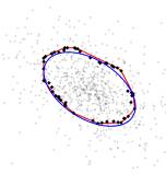
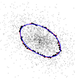
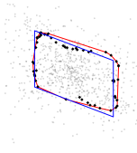
The set contains random points on the boundary of . It is shown in Lemma S36 that is small, which is allows us to control the error of the approximation of by . Figure 1 illustrates the behaviour of the algorithm when . Recall the definition of from (7); the next Proposition bounds the deviation .

Proposition 13.
Suppose that , , that there exist such that , and write . Suppose further that and let . Let and let be the output of Algorithm 1. Then, there exists a constant depending only on and such that with probability at least ,
| (10) |
-
Remark:
If is in an isotropic position, then we have that by John’s Ellipsoid Theorem (John, 1948, Section 3). If is additionally balanced, then we know from the same theorem that (see the remark after Proposition 11). Therefore, we recommend that Algorithm 1 be applied to whitened data where and are the sample covariance matrix and the sample mean respectively. This transformation brings into an approximately isotropic position, and the error in this approximation is given in Proposition 11.
- Remark:
Corollary 14.
-
Remark:
It is important to observe that the computation of the estimator is scalable for large and . Computing requires at most operations, since we represent implicitly in terms of its hull vertices and have no need to enumerate its facets. For any , we may then compute through a straightforward linear programme of at most variables; see (11). Thus, it is also fast to compute and to evaluate at any .
5 Algorithm
In this section, we assume , and data with empirical distribution are given, and describe an efficient algorithm for computing the -homothetic log-concave projection of . Fixing , we first note that in many cases of interest, the Minkowski functional is easy to compute when is constructed using the estimation schemes described in Section 4. In particular, if is of the form , where is a known convex body whose Minkowski functional is simple to compute, and where , as is the case in Section 4.2, then , so it may also be computed easily. As another example, if is the convex hull of a set of points in , as is the case in Section 4.3, then is the solution to the following linear programme:
| (11) |
Let for , and let denote the empirical distribution of . Proposition 4 shows that, provided at least one of is non-zero, the function is well-defined, and we can then set . Our aim is therefore to provide an algorithm for computing .
Let denote the set of with the property that is constant on the interval and affine on the intervals for , with for . Observe that if we fix , and be such that and for all . Then by concavity of , we have for all . Hence
| (12) |
The volume , in the case where where the volume of is known and , takes the simple form . More generally, can be computed efficiently if, for any , the query of whether or not can be evaluated efficiently. When is the convex hull of points in for example, we may evaluate a query by solving the linear programme (11) and then checking whether the solution is less than or equal to 1. If we let denote the number of queries made by an algorithm, then Kannan et al. (1997) give a Markov Chain Monte Carlo algorithm whose query complexity is bounded by up to polylogarithmic factors. In fact, the computation of the volume of a convex body is a deep and beautiful problem that had been studied intensely by the theoretical computer scientists since the seminal paper of Dyer et al. (1991), who first gave a polynomial time algorithm for the problem. It is one of few instances in computer science where all deterministic algorithms are provably intractable but efficient randomised algorithms exist. We refer readers to Simonovits (2003) for an accessible tutorial.
We now assume for simplicity of exposition that are distinct. The more general case can be treated similarly by assigning appropriate weights to duplicated points. Any can be identified with given by for . For , let . Define to have two non-zero entries, namely , . Further, for , let have three non-zero entries, namely
Finally, let . By (5), we see that it suffices to compute , where
| (13) |
This is a finite-dimensional convex optimisation problem with linear inequality constraints. We propose an active set algorithm for the optimisation of (13), a variant of the algorithm used in Dümbgen et al. (2007) to compute the ordinary univariate log-concave MLE. For , we define to be the set of ‘active’ constraints. Note that this is the complement in of the set of ‘knots’ of . Given a set , we define , and
| (14) |
Here, the maximiser is unique because is strictly concave on with as . It is convenient to define, for , vectors by
where, as usual, we interpret an empty sum as , and also define , the all-one vector. It follows from this definition that for and for all and with . Finally, given and , we define
We are now in a position to present the full algorithm; see Algorithm 2. It is guaranteed to terminate in finitely many steps with the exact solution.
Input: , , .
Output: .
We complete this section by providing further detail on how to solve the optimisation problem in (14). Given the active set , let us define . We index the elements of by where . Given , we also write for the matrix in obtained by extracting the rows of with indices in . Observe that the set is the subspace of where for , we have , and for , we have
It follows we can solve the optimisation problem (14) by solving instead an unconstrained optimisation over variables, i.e. by computing
We solve this latter problem via Newton’s method.
6 Empirical performance
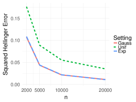
We perform three sets of simulation studies. In the first set, reported in Figure 2, we choose suppose that and are known. We generate where we take , and in settings (a), (b) and (c) respectively. We then compute the homothetic log-concave MLE and report the average squared Hellinger errors over 50 repetitions and with in the curve labelled “HLC” Figure 2. For comparison, we also present the corresponding results with in the curves labelled “HLC(p=100k)”. The simulation results are in line with Theorem 7, which gives a bound on that is independent of .


We also compare the -homothetic log-concave MLE against two alternative methods. In the first of these methods, we write for , apply the ordinary univariate log-concave MLE to to obtain a density and then estimate by , where
| (15) |
We compute the squared Hellinger errors and report them in the curve labelled in Figure 2. In fact, besides the improved empirical performance of observed in Figure 2, we argue that has several advantages over in this context, and list these in roughly decreasing order of importance:
- 1.
-
2.
As mentioned in Section 3.2, the estimator attains faster rates of convergence when the true density has a simple structure;
-
3.
The estimator takes values in the relevant class , whereas does not;
-
4.
The estimator exists in slightly greater generality than (cf. the remark following Proposition 4(iv)).


In the second competing method, we apply a kernel density estimator (with the default settings of the density function in R) to to obtain a density , and then estimate by , where . We compute the squared Hellinger errors and report them in the curve labelled ‘’ in Figure 2. The squared Hellinger errors for the kernel density estimator do not appear in Figure 2(b) because the errors are greater than 0.007 and therefore much larger than those of and .

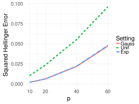
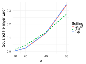
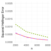
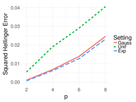
In the second set of simulations, reported in Figure 4, we consider the semiparametric setting where for some known and unknown . We estimate up to a scaling factor by the empirical covariance matrix , take to be , and estimate the centering vector (taken to be 0) by the empirical mean vector . We then construct for , compute , and construct the density estimate . In all cases, we generate as , where is generated according to Haar measure on the set of orthogonal real matrices, and where is a diagonal matrix whose th diagonal entry is . In Figures 4(a) and 4(c), we take , while in Figures 4(b) and 4(d), we take . In Figures 4(a) and 4(b), we fix and report the squared Hellinger errors for , while in Figures 4(c) and 4(d), we fix and report the corresponding squared errors with . In the settings of Figures 4(a) and 4(c), we see the advantage conferred by the smoothness of , in line with our theoretical guarantees from Corollary 12. On the other hand, when in Figures 4(b) and 4(d), is much larger than in the case (it is equal to instead of ), and this makes the problem significantly harder, which is again in agreement with Corollary 12.
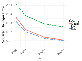
Finally, in the third set of simulations, given in Figure 5, we take to be known and estimate nonparametrically using Algorithm 1, with . As with the previous set of simulations, once we obtain , we construct for , compute , and set . The choices of were the same as those for in the corresponding panels of Figure 4. In Figures 5(a) and 5(b), we take and , while in Figures 5(c) and 5(d), we fix and take . We observe similar phenomena to those seen in the case where is known up to a positive definite transformation.


Supplementary material to ‘High-dimensional nonparametric density estimation via symmetry and shape constraints’
Min Xu and Richard J. Samworth
S1 Proofs from Section 2
Proof of Proposition 1.
(i) This follows from the assumption that .
(ii) This follows from, e.g., Rockafellar (1997, Corollary 9.7.1).
(iii) Let and suppose that . Then there exists such that by the second claim. Since is convex, we have that . Moreover, since contains an open neighbourhood of 0, we see that is an interior point of . Conversely, if is an interior point of , then there exists such that . Hence there exists with , so the conclusion follows from (ii).
(iv) See Royden and Fitzpatrick (2010, Proposition 14.24). ∎
Proof of Proposition 2.
Any density of the form for some , and is upper semi-continuous, and is log-concave by Proposition 1(iv). Moreover, writing for , we have
for all by Proposition 1(ii) and Proposition 1(iv). Hence is homothetic, as required.
Conversely, suppose that is an upper semi-continuous, homothetic and log-concave density on , so there exist a decreasing function , a set with and such that for every . Then in particular, . Since , there exists such that . Thus, and . By replacing with and with , we may therefore assume without the loss of generality that .
We now claim that is left continuous. To see this, let and let be a sequence such that . Then, for any . Since , we have
Since and , we have , so . We have thus shown that is left continuous and may define by for and, if , we define and for any . Notice that for any and any , we have if and only if .
We now set and for (with the convention that ). Then the function is well-defined on and moreover for any and any , we have
We therefore conclude that , and hence , as desired.
Now suppose that for some , and . Suppose further that is not a uniform density and that for some . Then, by the log-concavity of , there exist such that and . Let , , and note that . If satisfies , then and thus . If on the other hand , then since is upper semi-continuous. Thus,
| (S1.1) |
By the same reasoning, and we therefore have that . But, writing and , we also have , and moreover, . We deduce that , and ), that and that for all , as required.
If is a uniform density, then there must exist and such that for and for . Similarly, there exist and such that for and for . It follows that if and only if , so . We conclude that and for all , as required. ∎
Proof of Proposition 3.
For , define and let be a random vector, independent of , distributed uniformly on . We claim that as . To see this, let be a random vector distributed uniformly on and let be a Bernoulli random variable, where , independent of . Since is uniformly distributed on , we have that and thus .
We observe that since . Now, writing and for the characteristic functions of and respectively, we have that for all . We deduce that . Since
it follows that , as claimed.
Define , so that has density
for any . We deduce that whenever is non-zero and such that is continuous at ,
Thus, since is continuous Lebesgue almost everywhere, by Scheffé’s lemma, converges in distribution to a random variable with density . We conclude that , as desired. ∎
-
Remark:
Alternatively, we may prove the first claim in Proposition 3 by defining, for any , an operator of the form and then showing that is uniformly distributed on for any . One can then show that if then since .
-
Remark:
In fact, from this proof, we see that Proposition 3 holds more generally whenever is compact and star-shaped at the interior point , and is continuous Lebesgue almost everywhere.
Proof of Proposition 4.
(i) Fix . Observe that if , then . Otherwise , and then there exist such that . Hence,
(ii) Now suppose that and let . Then,
as .
(iii) Finally, suppose that . For , we have
so .
For , let . Then, since , we have for some . We also write and . Then by the concavity of ,
| (S1.2) |
If and , then
On the other hand, if and , then from (S1.2) we see that . We deduce that there exists , depending only on , and , such that
The existence of then follows from the proof of Theorem 2.2 in Dümbgen et al. (2011).
(iv) By the change of variable formula (e.g. Billingsley, 1995, Theorem 16.13), we have for all . The result then follows from (iii), specialised to the case . ∎
Proof of Proposition 5.
(i) For any , we may define by . The map is a bijection from to . Let . Then, for any , we have
This establishes that and thus proves scale equivariance.
(ii) For any , we have
| (S1.3) |
Choose small enough that . Since , we must have as , and hence, by reducing if necessary, we may assume that . Now, for ,
Hence, if , then we may apply the dominated convergence theorem to (S1.3) to take the limit as and reach the desired conclusion. On the other hand, if , then for every ,
The result follows.
(iii) Letting , this is a consequence of (ii).
(iv) Letting , this also follows from an application of (ii). ∎
Proof of Proposition 6.
The proof is very similar to (in fact, somewhat more straightforward than) the proof of Dümbgen et al. (2011, Theorem 4.5), so we focus on the main differences. We first observe that if and are defined on the same probability space, then
Taking such that , we have that . Hence, writing and for the distributions of and respectively, we deduce that . It follows that , and , so for , say. For such , we write and . Let be an arbitrary, strictly increasing sequence of positive integers. By extracting a further subsequence if necessary, we may assume that . First note that, by considering the function ,
Our next claim is that . To see this, recall the definition of the classes from the proof of Proposition 4, and let be such that . Since , we see from the proof of Proposition 4 that our claim follows. This means that .
Let . Our next claim is that for all . To see this, note by our first claim that we may assume without loss of generality that there exists such that . Then, for any ,
Since , we deduce that
as required.
These two claims allow us to extract a further subsequence that converges in an appropriate sense to a limit (in particular, this convergence occurs Lebesgue almost everywhere). It turns out that , that , and, writing , we have . The desired total variation convergence (6) follows. See the proof of Theorem 4.5 of Dümbgen et al. (2011) for details.
For the final claim, note that our previous argument allows us to conclude that converges to Lebesgue almost everywhere. The conclusion therefore follows from Rockafellar (1997, Theorem 10.8). ∎
S2 Proofs from Section 3
Proof of Theorem 7.
Let denote the density of , so that for some by Proposition 3. Let for , and write for the empirical distribution of . Now let , so that , where , by Proposition 4(iv). Then for , so . By scale equivariance of (Proposition 5(i)), together with the scale invariance of the loss function, we may assume without loss of generality that . By Lemma S5, there exist universal constants such that . Moreover, by Lemma S8, there exists a universal constant such that for every ,
Define , so that is decreasing. By choosing for a suitably large universal constant , we may apply Kim et al. (2018b, Theorem 10) (a minor restatement of van de Geer (2000, Corollary 7.5)), to deduce that there exists a universal constant such that for ,
where, to obtain the final inequality, we have applied Lemmas S9 and S10. ∎
Proof of Theorem 8.
Fix where and , let be the intervals on which is affine, with , and let . We work throughout on the probability 1 event that . Define and . Let be the set of indices of intervals with at least eight data points, and let . Define to be the set of upper semi-continuous functions such that is decreasing and concave for each , and such that for . Note that a function need not be globally decreasing and, in fact, need not be continuous on . Given any and , let for , and let . Now, for , define
and let whenever for some , and otherwise. Then, for any ,
| (S2.4) |
Arguing similarly to the second paragraph of Section 2.3, it follows that the function defined by is a density. Moreover, for , the function is a density. Writing , and , we deduce from (S2) that
| (S2.5) |
Now, since and for , we have
| (S2.6) |
For the third term in (S2), we have by Lemmas S9 and S10, that for (cf. (S2)),
| (S2.7) |
Finally, to bound the first term in (S2), for , let us first define , , , , and temporarily assume that . Note that , and for . It follows by Proposition 9, applied conditionally on , a simple extension of Jensen’s inequality using the fact that is concave on (e.g. Han et al., 2018, Lemma 2) and the fact that is increasing for ,
| (S2.8) |
To bound the first term of (S2), observe that by two applications of Jensen’s inequality,
| (S2.9) |
But
| (S2.10) |
Moreover, by three further applications of Jensen’s inequality, and using the fact that is concave for , we have
| (S2.11) |
where the last step follows from the fact that is increasing for . Combining (S2), (S2),(S2.7), (S2), (S2), (S2) and (S2), the result follows in the case .
Proof of Proposition 9.
By the scale equivariance described in Proposition 5(i), we may assume without loss of generality that . Define . By Lemma S11, if , then for every , it holds that
On the other hand, if , then by Lemma S8, for every , we have that
It follows that
Define , where the universal constant is chosen such that
Set for a universal constant to be chosen later. Then, because is non-increasing, we have
By choosing the universal constant sufficiently large, we can ensure that this ratio is larger than the universal constant required to apply Theorem 10 in the online supplement of Kim et al. (2018b) (a minor restatement of van de Geer (2000, Corollary 7.5)). We deduce from this result that there exists a universal constant such that for ,
| (S2.12) |
Moreover, by Lemmas S9 and S10, for ,
| (S2.13) |
It follows from (S2.12), (S2) and Lemma S5 that for ,
as required. ∎
S3 Proofs from Section 4
Proof of Proposition 10.
First, we note that since depend only on , they are independent of . Moreover, since , we may, by Proposition 2, rescale if necessary to assume without loss of generality that
| (S3.14) |
Once we prove the proposition with this assumption, the more general conclusion follows immediately from the fact that both and remain unchanged if we rescale . Under assumption (S3.14), the event defined in (8) then takes the form
| (S3.15) |
and we choose universal constants small enough that the conclusions of Lemmas S20, S21, S25, S26, S27, S31, S32, and S33 hold.
Note that, by Proposition 5(i), is scale equivariant. Thus, is by construction also scale equivariant and consequently, we may rescale if necessary to assume that, on event , we have that . Now let . By Lemmas S20, S21, S25, S26, and S27, together with the fact that for all densities , there exists universal constants such that on the event ,
| (S3.16) |
where and . We now claim that . To see this, fix any and . Then,
Since and were chosen arbitrarily, we have that and that as desired. The first part of the proposition then follows.
Proof of Proposition 11.
Since is location invariant, is location equivariant, and is also location invariant, we assume without loss of generality that . Moreover, is scale equivariant in the sense that if and we define for , let and , then . Since is also scale invariant in the sense that for any , we assume without loss of generality that . Thus, there exists such that .
For each , the random variable has a univariate log-concave density with mean and variance . By e.g. Feng et al. (2018, Proposition S2(iii)), we have for all integers . Then, by Bernstein’s inequality, there exists a universal constant such that
Let , so that .
Proof of Proposition 13.
Algorithm 1 is scale equivariant in the sense that for any , if we let for and let be the resulting outputs of Algorithm 1 on inputs and respectively, then . Since the left-hand side of (10) is invariant to scaling of , we assume without loss of generality that . We also assume that , which can be done without loss of generality by Proposition 2 and the fact that the left-hand side of (10) is invariant to the scaling of .
S4 Auxiliary lemmas
S4.1 Auxiliary lemmas for Section 2
Our first result, amongst other things, reveals the density of the random variable when has a density belonging to .
Lemma S1.
Let , , and let be integrable. Let and let . Then
Proof.
By transforming to if necessary, we may assume without the loss of generality that . Define a measures on by and for . We claim that . To prove the claim, first consider the case where for some . Then
| (S4.19) |
For , define . Now are finite measures on , and is a -algebra that contains by (S4.19). Hence . For a general , we have that
and we deduce that , as claimed.
Now suppose that is a non-negative measurable function, fix and . Let be a sequence of non-negative, simple functions on such that , so that by our claim. By two applications of the monotone convergence theorem, we conclude that . The case where is integrable can be handled by applying this result to the positive and negative parts of . ∎
S4.2 Auxiliary lemmas for Section 3
The aim of the next three results is to elucidate the way in which the first two moments of the empirical distribution of a set of data points in change under the projection . These results enable us to show that if the data are drawn independently from a common distribution on , then with high probability, the first two moments of are close to their population analogues.
Our first lemma concerns bounds on , and is expressed in terms of the function defined by
| (S4.20) |
Basic properties of the function are given in Lemma S49.
Lemma S2.
Fix , and suppose that are real numbers in the interval that are not all equal to . Let be the empirical distribution corresponding to . Let , so that for , for some . Then, writing , as well as and , we have
Proof of Lemma S2.
By (5), we have that for some because is an empirical distribution. Moreover, the right derivative of at is strictly negative. Hence, by Proposition 5(ii), applied to the functions , we have
| (S4.21) |
Now, since for all , we have
We deduce that
| (S4.22) |
where we used Lemma S50 to obtain the final bound. From (S4.2) and (S4.2), we find that
| (S4.23) |
In particular, .
We now study bounds for , and their consequences for .
Lemma S3.
Let and let . Suppose that there exists such that . Let , and . Then there exists a universal constant such that
Moreover,
| (S4.25) |
Proof of Lemma S3.
We have
Since is upper semi-continuous, there exists such that . By Lemma S47(ii), we then have that for some universal constant .
To provide the lower bound for , we first prove (S4.25). To that end, let and let . If , then the claim immediately follows, so let us thus assume . Define and suppose first that . Then,
where the final inequality follows because the univariate function is concave and thus for any ; we take and to be and respectively. Thus,
| (S4.26) |
If on the other hand, , then we may use Dümbgen et al. (2011, Lemma 4.1) and the assumption that to obtain
and thus (S4.26) also follows. Therefore (S4.25) holds in all cases. By Lemma S47(i), there exists a universal constant such that , as desired. ∎
Lemma S4.
Let be a density on and suppose . Let with empirical distribution . We have that
Proof.
We may assume that since the bound is trivially true otherwise, and we also assume that are distinct (an event of probability 1). Let and denote the distribution function of and respectively. Define the event and observe that by the Dvoretzky–Kiefer–Wolfowitz inequality. On the event , for any with and , we have that
Thus, we have that and hence
as desired. ∎
We are now in a position to argue that, with high probability, belongs to a subclass of with restricted first two moments. These moment restrictions are important for enabling us to obtain the bracketing entropy bounds that drive the rates of convergence of the -homothetic log-concave MLE. For , and , let
| (S4.27) |
Lemma S5.
Let , fix a density with , and suppose that , with empirical distribution . Writing , there exist universal constants such that
Proof of Lemma S5.
We may assume that . Let , so that , by Chebychev’s inequality. On the event , we have by Lemma S2. Recall the definition of from Lemma S2. If , then by Lemma S2, on the event ,
where the middle inequality uses the fact that (Lemma S49(iii)). If , then by Lemma S2, on the event ,
Hence, if , then by Lemma S6, we have . On the other hand, if , then by Lemma S2,
It follows that there exists a universal constant such that
To bound , define the event . By Lemma S48 and Bobkov and Madiman (2011, Theorem 1.1), for ,
Define event . By Lemma S4, we have that . On the event , by Lemma S3 and S47, there exists a universal constant such that . The desired result follows from a union bound. ∎
The mean of any is constrained because for and some decreasing function . The next lemma formalises this notion.
Lemma S6.
Let and let . Then, writing , we have
- Remark:
Proof.
We initially assume that and write . If , then for and thus, . For the upper bound on , we first observe that by Lemma S47. Since is decreasing by Lemma S49(ii) and by Lemma S49(iii), we have that . Suppose for a contradiction that . Then, since is increasing by Lemma S49(i), we have for all . Moreover, by definition of , we have for all . Hence . But then Lemma S7 establishes a contradiction, so , as desired. For general , we apply the above argument to , which satisfies and . ∎
The next lemma is used in the proof of Lemma S6.
Lemma S7.
For any , and any , For any , ,
Proof.
Let us fix and define . Observe that is a density of the form for some . We will show that for all and if is such that , then (such an exists by the upper semi-continuity of ). The lemma then follows since .
To this end, fix and define where . Then
Hence , as desired.
To prove the second claim, fix such that . Observe that if , then and lemma follows. We may therefore assume that , define and fix . For , let . Since is itself a log-concave density, we have that, any and ,
Hence
Using Fubini’s theorem as in Dümbgen et al. (2011, Lemma 4.1), we can now compute
Since is an interval containing , we conclude that whenever . Thus, for , we have
Assume for the sake of contradiction that . Then
This is a contradiction since we assumed that . Thus . We deduce that
Since , we obtain as desired. ∎
The next lemma is a very slight generalisation of (Kim and Samworth, 2016, Theorem 4) and can be proved in the same manner, with minor modifications to handle the general mean and variance perturbation. The proof is omitted for brevity.
Lemma S8.
Kim and Samworth (2016, Theorem 4) Fix and . There exists , depending only on , such that for every ,
Lemma S9.
Let and let with and empirical distribution . Let . Then for and ,
Proof.
Let denote the empirical distribution of and define the event
Observe that occurs only if, for every closed interval of length at most , it holds that . Since by Feng et al. (2018, Proposition S2(iii)), we have that for ,
Lemma S10.
Let , let with , and suppose that . Writing and , there exists a universal constant such that for ,
Proof.
This result follows from the proof of Kim et al. (2018b, Lemma 2). ∎
S4.2.1 Local bracketing entropy results
For and , let
Recall from the introduction that denotes the class of all upper semi-continuous, log-concave densities on . For , we define
| (S4.28) |
where we adopt the convention that .
Lemma S11.
Fix and let . Assume that . Then there exists a universal constant such that, for all and all ,
Proof.
Fix with and let . Then, by the triangle inequality,
Since where , we have that is concave for any . We therefore have
where the right-hand side is defined in (S4.28). It then follows from this and Lemma S13 that
Since the choice of with was arbitrary, the bound continues to hold when is replaced with . ∎
Recall that denotes the set of all upper semi-continuous log-concave densities on .
Lemma S12.
Let . Then there exist universal constants such that if , then
Proof.
Since the Hellinger distance is affine invariant, we may assume without loss of generality that and . By Lovász and Vempala (2007, Theorem 5.14(a) and (d)), for . We claim that for some . To see this, suppose for a contradiction that for all . Then
a contradiction. By Lemma S47, it follows that for some universal constant . The lower bound on follows by symmetry.
Now assume without loss of generality that . By the first part and Feng et al. (2018, Proposition S2(iii)), for all . It follows that if , then
a contradiction. The result follows. ∎
We now prove a general result on the local bracketing entropy of log-concave densities.
Lemma S13.
Let and . Then there exists a universal constant such that, for every ,
Proof.
In this proof, we let be a generic universal constant whose value may vary from instance to instance. For a set , we define and abuse notation slightly to define . We note that, for any and disjoint Borel measurable sets ,
Since is location and scale equivariant, we assume without loss of generality that and . Define and ; it holds by the fact that and Lemma S16 that and . By Lemma S12 and Feng et al. (2018, Proposition S2(iii)), there exist and such that for any and , we have . Let and . Then, for any , for , and .
First, we will bracket the region . To this end, fix , and let and , so that . By these definitions, and . We segment into subintervals for , where
Define . For any , we have that because and, moreover, because . Now, by Lemma S15, for any and . Hence, by Lemma S18,
| (S4.29) |
By symmetry, we obtain the same bound for .
Now we bracket the region . For , define and set where is a constant chosen such that . Then, by Lemma S18 again,
| (S4.30) |
The same bound holds for .
Next, we bracket the region . To this end, we write and partition into segments , , (where ) as follows:
-
1.
Choose such that .
-
2.
For each , if there exists such that , then choose such that . Otherwise, set and choose .
Define and write . We make the following six claims:
-
(1)
;
-
(2)
;
-
(3)
;
-
(4)
for ;
-
(5)
;
-
(6)
.
To verify claim (1), observe by Lovász and Vempala (2007, Theorem 5.14(a) and (d)) that for all . Hence , so .
For claim (2), note that for by Feng et al. (2018, Proposition S2(iii)). Thus by the second part of Lemma S17 and the definition of , we have
For claim (3), we have .
For claim (5), we have
Finally, for claim (6), we have
so .
Now let , and observe by claim (1) that are strictly increasing. Let . Let be an -Hellinger bracketing set for with ; we define by and . Then
Moreover, if , then . We deduce that form an -Hellinger bracketing set for .
Now, on , the conditions of Lemma S14 are fulfilled with because and by claim (3). Thus, we may combine Lemma S19 with Lemmas S14 and S15 with claim (4) to obtain
| (S4.32) |
where the final bound follows because by Markov’s inequality.
By symmetry, we obtain the same bracketing entropy bound over . For the region , since and by claim (5), we may argue as in (S4.2.1) to obtain
| (S4.33) |
Now, since is unimodal and on , it holds that
Thus, by Jensen’s inequality,
| (S4.34) |
We conclude from (S4.34), (S4.33), (S4.2.1), (S4.2.1), (S4.2.1), (S4.2.1) and claim (6) that
as required. ∎
Lemma S14.
Let for some concave and and let . If , then
Proof.
As a shorthand, let us write . Assume without loss of generality that (because otherwise the result is immediate). Since is concave, either for all or for all . In the former case,
Hence
On the other hand, if for , we can apply an almost identical argument to see that
as required. ∎
Lemma S15.
Let with and , and let for some . Then there exists a universal constant such that for any ,
Proof.
Again, we write . Since we seek an upper bound for , we may assume without loss of generality that is upper semi-continuous, and by symmetry, it suffices to prove the bound at a fixed . Further, we assume without loss of generality that (because otherwise the result is immediate).
Let . Define , , and . We note that since . Then, since for any , we have
| (S4.35) |
Now, define , , and . Then
| (S4.36) |
As a shorthand, let us define
Inequalities (S4.35) and (S4.36) yield
| (S4.37) | ||||
| (S4.38) |
Since , we have that by Lemma S16.
We claim that . To see this, note that by concavity of (cf. the proof of Theorem 1 of Cule et al. (2010)),
By Feng et al. (2018, Proposition S2(iii)), , hence,
It follows that either or . If , then the result follows from (S4.37). On the other hand, if , then we obtain the desired result from the fact that , that for all , and (S4.38). ∎
Lemma S16.
Let be such that and . We have that , , and
| (S4.39) |
Proof.
By Lovász and Vempala (2007, Theorem 5.14(a) and 5.14(d)), and for all . We immediately obtain that and . Moreover,
as required. ∎
Lemma S17.
Let be a concave function, let where , and let
Then for any , it holds that
Moreover, if for some , then
Proof.
Let us first suppose that . We have for , where . Hence
| (S4.40) |
We can bound when by a similar argument to yield the first conclusion.
For the second part, observe that is strictly decreasing, so from (S4.40),
for . We may bound by a similar argument to obtain the desired conclusion. ∎
The following two lemmas are from Kim et al. (2018a), though the first is only a minor restatement of Doss and Wellner (2016, Theorem 4.1). For and , we define to be the set of log-concave functions .
Lemma S18.
There exists a universal constant such that
for every and
Lemma S19.
There exists a universal constant such that
for every , and .
S4.3 Auxiliary lemmas for Subsection 4.1
We first describe the common setting for all the lemmas in this subsection and define the notation used throughout. We fix , Let be of the form for some and let . We assume in this subsection that
| (S4.41) |
This assumption can be made without loss of generality as shown in the proof of Proposition 10. Let be a density on be of the form . Define by . We note that is not necessarily a density. Let
| (S4.42) |
We also define a deformation of by
| (S4.45) |
and write where so that is a density.
For , let and . Then has density and, by Lemma S24 below, has a density which we denote by . We let and denote the probability distributions induced by and respectively and let denote the empirical distribution corresponding to , so that . We write for some , and set . Similarly to (S4.27) we write .
Lemma S20.
There exist universal constants and such that if and , then
Proof.
The proof is similar to that of Lemma S5.
As a preliminary step, we first claim that there exist universal constants such that if and , then the following statements hold simultaneously:
| (S4.46) | |||
| (S4.47) |
Provided we choose universal constants sufficiently small, claim (a) follows from Lemma S28, while claim (d) follows from the second claim of Lemma S26 and Lemma S12. For claim (b), observe that since (which holds by Lemma S6), we have that . Thus, by Lemma S22, we may reduce the values of if necessary to obtain
| (S4.48) |
For claim (c), observe that . We therefore have by Cauchy–Schwarz and claim (b) that,
| (S4.49) |
and
This establishes claim (c).
Define ; from claim (c) of (S4.47) and Chebychev’s inequality, it holds that . By Lemma S2 (with ) and claim (b) of (S4.47), there exists a universal constant such that on ,
| (S4.50) |
Similarly, by Lemma S2 again and Lemma S6,
| (S4.51) |
We therefore conclude that
| (S4.52) |
We now consider . By Lemma S23, S47, and claims (a) and (d) of (S4.47), there exists a universal constant such that . Define the event
Then by Lemma S4.
We now obtain a lower bound for . Note that by Cover and Thomas (2006, Theorem 8.6.5) and by claim (c) of (S4.47), we have that
| (S4.53) |
Now write for as a shorthand and observe that
| (S4.54) |
By claim (d) of (S4.47) and Feng et al. (2018, Proposition S2(iii)), there exist universal constants such that for all . Thus, by claim (a) of (S4.47), for any ,
| (S4.55) |
Combining (S4.54) and (S4.55), we deduce that there exists a universal constant such that
| (S4.56) |
Therefore, we have by (S4.56) that
| (S4.57) |
Defining the event
we have by (S4.57) and Chebychev’s inequality that . Let and let denote the event that and . It holds then by Lemma S23 that .
Moreover, on ,
| (S4.58) |
for some universal constant . We conclude that on the event , by Lemma S3, there exists a universal constant such that
A union bound yields the desired result. ∎
For a Borel measurable function , define
Even though is not a norm, we can define the -generalised bracketing entropy of a class of Borel measurable, real-valued functions by treating it as a norm, and continue to denote this by .
Lemma S21.
Proof.
Assume and for universal constants chosen such that (a) where and are taken from Lemma S20 and (b) . The existence of such a choice of is guaranteed by Lemma S12, Lemma S26, and Lemma S28.
We make two observations before proceeding with the main proof. First, for , define , and observe that for every . Second, we may assume that (since this is a probability 1 event), and thus, and (recall the definition of in (4)). Therefore, since , we have by Proposition 4 and Lemma S23 that with probability 1,
Hence, again with probability 1,
| (S4.60) |
Now we proceed to the proof of the Lemma. We have
| (S4.61) |
To bound the first term, we have by Lemma S1 that
| (S4.62) |
By van de Geer (2000, Lemma 4.2), the fact that KL divergence is no smaller than the squared Hellinger distance, and (S4.60),
| (S4.63) |
Since is nonempty for any , the bracketing entropy is well-defined and non-negative for any . We may therefore define by and let for a universal constant specified in van de Geer (2000, Theorem 5.11). By Lemma S8, it holds that . Moreover, if for some and , then, by Lemma S11, we have that .
For , define . Let be an element from the -Hellinger bracketing set of . Define and . We have by van de Geer (2000, Lemmas 7.1 and 4.2), Lemma S23 and the fact that that
| (S4.64) |
Moreover, if and , then a virtually identical calculation to (S4.3) shows that for every . We therefore conclude that
| (S4.65) |
Fix any , where we note that this lower bound is finite by Lemma S23. For each , define the events . Writing , we note that on , by (S4.3),
| (S4.66) |
Moreover, since is decreasing, we have
and thus, by (S4.65),
| (S4.67) |
Therefore, by (S4.66), (S4.67), and van de Geer (2000, Theorem 5.11), there exists a universal constant such that
| (S4.68) |
The lemma follows from (S4.61), (S4.3), (S4.68), and the fact that in general and when has the form for some and . ∎
Lemma S22.
Let and let . Writing , we have
Proof.
By the subadditivity of (Proposition 1(iv)), we have
and
This yields the bound with the first term in the minimum, and the bound with the second term follows analogously. ∎
Lemma S23.
For every , we have that . Moreover, for -almost every , we have that .
Proof.
Let . If , then, since is decreasing, . On the other hand, if , then
Hence, . This proves the first claim of the lemma.
For , we write . Then, by the first claim of the lemma and Lemma S1, for any and ,
| (S4.69) |
We now take the limit as on both sides. On the left-hand side, we may apply Lemma S24 to conclude that the limit is for -almost all . On the right-hand side, the limit is whenever is a continuity point of (i.e. -almost everywhere, since is decreasing). ∎
-
Definition:
Let be a signed measure on and let . We refer to the signed measure on defined by for as the -contour measure of .
The following lemma, among other things, implies that if a random vector has a density on , then has a density on as well.
Lemma S24.
Let be a signed measure on with . Let and let be the -contour measure of . Then .
Proof.
Define by . We first claim that for any Borel measurable such that , we have .
Let be a Borel measurable set such that , let , and let . Now let be fixed. Since , there exist disjoint intervals such that and . Then by the mean value theorem, for any ,
We therefore deduce that
Since was arbitrary, , so , which establishes the claim.
Hence, if is a Borel measurable subset of with , then since , we have , as required. ∎
S4.3.1 Auxiliary lemmas for the worst case risk bounds of Section 4
We continue to use the setting and notation defined in Subsection S4.3.
Lemma S25.
If and , then
Proof.
By Fubini’s theorem,
| (S4.70) |
For any and , define and define analogously. Define by for any . Since if and only if for any and , we have
| (S4.71) |
Let us denote and so that, for any , we have . To upper bound the first term of (S4.71), we obtain from the translation invariance of Lebesgue measure, its corresponding scaling property and Proposition 1(iv) that
| (S4.72) |
To upper bound the second term of (S4.71), note that by the translation invariance of Lebesgue measure again,
| (S4.73) |
Combining (S4.3.1), (S4.71), (S4.72) and (S4.73), we obtain
| (S4.74) |
Recall that and . We now make a few observations that are used repeatedly in the remainder of this proof:
-
(i)
By Feng et al. (2018), it holds that for all .
- (ii)
-
(iii)
Since , we have .
-
(iv)
From (ii) and (iii) as well as Lemma S6, there exists a universal constant such that .
Suppose first that . Define ; we observe that since . We also define by
We then have that
| (S4.78) |
Since , we see that is a decreasing function and, since , we also have that for all . We now claim that
| (S4.79) |
To see this, note that if , then as required. On the other hand, suppose that . Then by the proof of Lemma S47,
and moreover,
From the fact that as , we deduce that there exists a universal constants such that
| (S4.80) |
Therefore, we also obtain in this case that
Define by . It follows from the fact for all that for all . Hence, by a change of a variable and our assumption on ,
where the final inequality follows from (S4.79). Now define and note that
Hence
| (S4.81) |
Returning to (S4.74), by a very similar argument, we also have that
| (S4.82) |
It follows from (S4.74), (S4.81) and (S4.82) that
as desired. If , then we define
| (S4.85) |
and observe, as in the case when , that is decreasing, that for all , and that for and for . By applying the same argument as for the case where , we obtain the conclusion of the lemma. ∎
Lemma S26.
If and , then
and
Proof.
Lemma S27.
If and , then
Proof.
By Lemma S23, the fact that for all , and the fact that ,
By Lemma S25, Lemma S28, and (S4.92) in the proof of Lemma S28, we have that
| (S4.86) |
We observe that is the density of the -contour measure (see definition above Lemma S24) of the probability measure induced by . By (S4.86) and Lemma S30, it holds that
as desired. ∎
Lemma S28.
If and , then
Proof.
By the definition of and Lemma S29,
| (S4.87) |
We define by and ; we also write . Observe that for any and , so . By Fubini’s theorem,
| (S4.88) |
Let us first assume and define , , and as in the proof of Lemma S25. Recall from the proof of Lemma S25 that for all . Since , it also holds that for all . We may now follow the proof of Lemma S25 and apply the assumption on and a change of variable to obtain
| (S4.89) |
Now, in order to bound the first term of (S4.89), we use (S4.79), the assumptions on and , and the fact that to obtain
| (S4.90) |
To bound the second term of (S4.89), we again follow the proof of Lemma S25 and use (S4.81) and (S4.82):
| (S4.91) |
From (S4.3.1),(S4.89), (S4.3.1) and (S4.3.1), we deduce that
| (S4.92) |
The desired result therefore follows from (S4.87).
Lemma S29.
If , then
Proof.
We first prove the upper bound on . Since for , we have
when , as required.
For the lower bound on , by the fact that for , we have
as required. ∎
Lemma S30.
Let and let be a density on with corresponding distribution . Let be the density of the -contour measure (see Definition before Lemma S24) of . Let be a continuous function such that and suppose that
| (S4.93) |
Then
Proof.
By condition (S4.93), we may define a signed measure on by for any Borel measurable . Let denote the -contour measure of . Since , we have by Lemma S24 that . Let denote the Radon–Nikodym derivative of with respect to . For any and , define .
We observe that, by (S4.93) and the fact that the integral in that assumption is also non-negative by the Gibbs inequality, is locally bounded on in the sense that for every bounded and therefore, is locally bounded on . Then, by the Lebesgue differentiation theorem (Folland, 2013, Theorem 3.21), for -almost every ,
Moreover, we claim that . To see this, let be such that . Then, by definition of , we have that is -almost everywhere on and thus we conclude that as well, which establishes the claim. By (S4.93) again, it must be that and thus . Hence, we have that for -almost every such that .
For , let us define
and define . For any such that , we have by continuity of that
so -almost everywhere.
We also observe that is locally bounded since is a density. Thus, is locally bounded and consequently, there exists such that for every and . Fix and with . Since is convex on (with the convention that ), we have by Jensen’s inequality that
| (S4.94) |
S4.3.2 Auxiliary lemmas for the adaptive risk bounds of Section 4
Lemma S31.
Suppose that and that . If is absolutely continuous and differentiable, and there exists such that , then
Proof.
We have by absolute continuity of that
| (S4.95) |
For any , the function is a density on . Moreover, since the function is finite when integrated over , we may, by Ash and Doleans-Dade (1999, Exercise 1.6.3), differentiate under the integral to obtain
| (S4.96) |
where the final inequality follows from Bobkov (2003, Lemma 1). From (S4.95) and (S4.3.2), we deduce that
| (S4.97) |
Using the inequality for , and writing , we have
| (S4.98) |
As a shorthand, write , and . By Lemma S22, Taylor’s theorem, and the facts that and by our assumption on , we have that
| (S4.99) |
By (S4.3.2), Lemma S1, (S4.97) and Lemma S34, we have that
| (S4.100) |
Similarly, by Lemma S29,
| (S4.101) |
where the final inequality follows because and . Combining (S4.98), (S4.100) and (S4.101) yields the desired conclusion. ∎
Lemma S32.
There exists universal constants such that if and and if is absolutely continuous and differentiable and there exists such that , then
and
Proof.
We first note that (S4.97) holds since we have the same assumptions on as Lemma S31. Define by
| (S4.104) |
so that . For , write . By Lemma S1 and the inequality for ,
| (S4.105) |
Let us write . Since , we have by Taylor’s theorem that
Now, write , and note that . By Lemma S28 and the fact that (a consequence of Lemma S23), we have that
| (S4.106) |
Therefore, we have by Lemma S1, (S4.97), Lemma S34, (S4.106), and Lemma S29 that
| (S4.107) |
Similarly, but using Lemma S35 instead of Lemma S34, we have that
| (S4.108) |
The first statement of the lemma then follows from (S4.105), (S4.3.2) and (S4.3.2). For the second statement, note that, by our assumption on ,
as desired. ∎
Lemma S33.
There exists universal constants such that if and that and if is absolutely continuous and differentiable and there exists such that , then
Proof.
First, we observe that, by Lemma S23 and S28,
| (S4.109) |
We also observe that is the density of the -contour measure of the probability distribution induced by .
As a shorthand, for , let
Then, by Lemma S30 (which is applicable by (S4.109)) and the fact that for any , we have
Define for . By the fact that for all , by Lemma S23, and by Lemma S28,
where we used (S4.101) and (S4.3.2) to obtain the final inequality. The lemma therefore follows from our assumption on . ∎
Lemma S34.
For any ,
Proof.
Lemma S35.
There exists a universal constant such that if and , then
S4.4 Auxiliary lemmas for Section 4.3
We first describe the common setting for all the lemmas in this subsection as well as define some notation and quantities used throughout. We fix , and ; we assume, for some fixed , that and write . We suppose that . Recall from Algorithm 1 then that for . Define
| (S4.110) |
For , we also define
Note that with this definition, for any , the random quantity as defined in Algorithm 1 satisfies . For , define the spherical cone with centre as . We then define the events
| (S4.111) |
For , we say that a finite set is an -net of if for every , there exists such that .
The key results of this subsection are Lemmas S36 and S43, both of which are used in the proof of Proposition 13.
Lemma S36.
Suppose that and that . For , let be defined as in Algorithm 1. Then there exists , depending only on and , such that, with probability at least ,
Proof.
For , let . We have that under our assumptions on . Thus, on the event , we have by Lemma S39 that
and that
and therefore
| (S4.112) |
Define the event . To bound , choose with . Let be the event that . Then, by Proposition 3 and Karlin et al. (1961, Theorem 5), for any ,
| (S4.113) |
By Proposition 3 again, Bernstein’s inequality (Boucheron et al., 2013, Corollary 2.11), and the fact that under our assumption on and , we therefore have that for each ,
Hence, for each ,
Thus, using a union bound over , Lemma S38 (which we may apply since under our assumption on ), and the fact that ,
| (S4.114) |
Now, under the assumption that , we have . Moreover,
so . Thus, on the event , for each ,
Finally, by Lemma S37 and (S4.114), there exists , depending only on and , such that as required. ∎
Lemma S37.
If , then there exists , depending only on and , such that
Proof.
Let . By Lemma S41, there exists an -net of such that for some depending only on . Let be the event that for every , there exists some such that . By Lemma S40 and a union bound, we have that
| (S4.115) |
say. Now for any , there exist such that for , that for any and that for . Thus, on the event , for any , there exist not equal to such that . Thus, on the event , we have for every .
Now let and note that . For any , let . Let be the event that . Then by Lemma S40 again,
| (S4.116) |
say. On the event , we have for every . Setting and applying a union bound, we obtain the conclusion of the lemma as desired. ∎
Lemma S38.
If and , then there exists , depending only on and , such that
| (S4.117) |
Proof.
Lemma S39.
Let and let . Then, for all , we have
Proof.
The claim is immediately true if or if . Thus, let be such that and . Let , so that . Then
The claim then follows from the fact that . ∎
Lemma S40.
Let be a random vector uniformly distributed on . Let be fixed and let . Then,
where are as defined in (S4.110).
Proof.
Fix and let so that is the base of the spherical cap . Define also . We observe then that
We therefore have that
For the lower bound, we have
as desired. ∎
The following lemma is well-known and follows from the fact that the surface area of a spherical cap scales as up to a multiplicative constant depending only on (Li, 2011). We omit the proof for brevity.
Lemma S41.
There exists , depending only on , such that, for every , there exists an -net of of cardinality .
For , let be the support function of , i.e., for . For any and , define . For , we define the Hausdorff distance .
Theorem S42.
(Brunel, 2018b, Theorem 1) Let with and let be probability distribution supported on . Suppose there exist , and such that for all . Let be independent random vectors with distribution and let . Let and . If , then
Lemma S43.
Let be independent random vectors distributed uniformly on . Let for , and let . If , then
Proof.
Since is scale invariant, we assume without loss of generality that so that . Let denote the distribution of . We claim that satisfies the hypothesis of Theorem S42 with , , and .
To see this, let and be arbitrary and let be such that . We write . Let be the base of and define and . Let be the conical pyramid connecting and and let . Then, by an application of Corollary S45, the fact that , the fact that , and the fact that ,
Let and be defined as in Theorem S42. Since we have that . Moreover, and so . By the assumption on , we have that . Thus, writing
we have by Theorem S42 that
| (S4.119) |
We now work on the event , which by our assumption on implies that . We can therefore fix . Since , we have . Applying this recursively, we obtain for any . Because , it holds that for any , there exists such that , and . Thus, for all and so is a limit point of . Since is closed, we conclude that and hence that . On the other hand, we have that by definition and so . Since was chosen arbitrarily, we have that on the event ,
as desired. ∎
Recall that for , the -dimensional Hausdorff outer measure of is defined as
| (S4.120) |
Note that by this definition, if is Lebesgue measurable, then (e.g., Mattila, 1999, Section 4.3). We extend the definition of to Borel subsets of by writing for a Borel measurable . The next lemma shows that the Hausdorff measure contracts under a -Lipschitz map.
Lemma S44.
Let be a -Lipschitz mapping in the sense that for any , . For , let be the -dimensional Hausdorff outer measure as defined in (S4.120). Then, for any ,
Proof.
For any , we have that . The claim follows immediately. ∎
Corollary S45.
Let be compact convex sets with non-empty interiors. If , then, .
Proof.
For any , let denote the Euclidean projection onto . To see that is -Lipschitz, let and let and . If then certainly . On the other hand, if , then, by the optimality conditions of ,
We may then apply the Cauchy–Schwarz inequality to obtain that .
If , then because otherwise we can find a point in on the line segment between and that is closer to than is . Thus, . For any , by the separating hyperplane theorem (e.g. Rockafellar, 1997, Theorem 11.6), there exists and such that and for all . Since , there exists such that for some . Moreover, for any ,
so . Thus, and the result follows from Lemma S44. ∎
Recall the definition of from (7).
Lemma S46.
We have
-
1.
for any .
-
2.
For any such that or , it holds that .
Proof.
The first claim follows from the fact that if and only if .
For the second claim, let , and suppose without loss of generality that . Then there exist and such that and . Since
we have that . Since this holds for any and , the claim follows. ∎
S5 Technical lemmas
Lemma S47.
Let .
-
(i)
There exists a universal constant such that ;
-
(ii)
There exists a universal constant such that .
Proof.
(i) Let , so is a log-concave density with and . Then
where the final inequality follows from Lovász and Vempala (2007, Theorem 5.14(d)).
(ii) Since is upper semi-continuous and as , there exists such that . Thus, with as above,
by Lovász and Vempala (2007, Theorem 5.14(b) and (d)). ∎
Lemma S48.
For any with , we have that
Proof.
By the location invariance of the entropy functional, we may assume without loss of generality that . Since (Lovász and Vempala, 2007, Theorem 5.14(b) and (d)), we have
Now let , so by the non-negativity of Kullback–Leibler divergence,
as required. ∎
The next lemma provides basic properties of the function defined in (S4.20).
Lemma S49.
For any and , we have
-
(i)
is increasing;
-
(ii)
is decreasing;
-
(iii)
for all .
Proof.
If , define , an increasing function of . Then
which is increasing in , as required. If , then , so the claim is also true.
If , then
which is decreasing in . If , then and the claim also follows.
When , the result follows because for all . When , the lower bound follows from and the fact that , while the upper bound follows from and the fact that . ∎
Lemma S50.
For any and , we have that
Proof.
Writing , we are required to prove that for ,
| (S5.121) |
The inequality holds for sufficiently small and at , and also when . To finish the proof, it suffices to show that is concave on when . But for ,
as required. ∎
Lemma S51.
Let and . Then
Proof.
By Taylor’s theorem, there exists on the line segment joining and such that
The lemma follows by noting that . ∎
References
- (1)
- Adamczak et al. (2010) Adamczak, R., Litvak, A., Pajor, A. and Tomczak-Jaegermann, N. (2010). Quantitative estimates of the convergence of the empirical covariance matrix in log-concave ensembles, J. Amer. Math. Soc. 23: 535–561.
- Ash and Doleans-Dade (1999) Ash, R. B. and Doleans-Dade, C. A. (1999). Probability and Measure Theory, 2nd Edition, Academic Press, San Diego, CA, USA.
- Ball (1997) Ball, K. (1997). An elementary introduction to modern convex geometry, in S. Levy (ed.), Flavors of Geometry, Vol. 31, Cambridge University Press, Cambridge, UK, pp. 1–58.
- Bhattacharya and Bickel (2012) Bhattacharya, S. and Bickel, P. J. (2012). Adaptive estimation in elliptical distributions with extensions to high-dimensions, Preprint. Available at http://www.science.oregonstate.edu/~bhattash/Site/Research.html .
- Biau and Devroye (2003) Biau, G. and Devroye, L. (2003). On the risk of estimates for block decreasing densities, J. Mult. Anal. 86: 143–165.
- Billingsley (1995) Billingsley, P. (1995). Probability and Measure, Wiley, New York.
- Bobkov (2003) Bobkov, S. G. (2003). Spectral gap and concentration for some spherically symmetric probability measures, Geometric aspects of functional analysis, Springer, pp. 37–43.
- Bobkov and Madiman (2011) Bobkov, S. and Madiman, M. (2011). Concentration of the information in data with log-concave distributions, Ann. Probab. 39: 1528–1543.
- Boucheron et al. (2013) Boucheron, S., Lugosi, G. and Massart, P. (2013). Concentration Inequalities: A Nonasymptotic Theory of Independence, Oxford University Press, Oxford, UK.
- Bronstein (2008) Bronstein, E. M. (2008). Approximation of convex sets by polytopes, J. Math. Sci. 153: 727–762.
- Brunel (2018a) Brunel, V.-E. (2018a). Methods for estimation of convex sets, Statist. Sci. 33: 615–632.
- Brunel (2018b) Brunel, V.-E. (2018b). Uniform behaviors of random polytopes under the Hausdorff metric, Preprint ArXiv:1503.01504 .
- Carpenter et al. (2018) Carpenter, T., Diakonikolas, I., Sidiropoulos, A. and Stewart, A. (2018). Near-optimal sample complexity bounds for maximum likelihood estimation of multivariate log-concave densities, Proc. Mach. Learn. Res. 75: 1–29.
- Cover and Thomas (2006) Cover, T. M. and Thomas, J. A. (2006). Elements of Information Theory, Wiley-Interscience, New York, NY, USA.
- Cule and Samworth (2010) Cule, M. and Samworth, R. (2010). Theoretical properties of the log-concave maximum likelihood estimator of a multidimensional density, Elect. J. of Statist. 4: 254–270.
- Cule et al. (2010) Cule, M., Samworth, R. and Stewart, M. (2010). Maximum likelihood estimation of a multi-dimensional log-concave density, J. Roy. Statist. Soc., Ser. B (with discussion) 72: 545–607.
- Dagan and Kur (2019) Dagan, Y. and Kur, G. (2019). The log-concave maximum likelihood estimator is optimal in high dimensions, Preprint ArXiv:1903.05315 .
- Donoho et al. (1996) Donoho, D. L., Johnstone, I. M., Kerkyacharian, G. and Picard, D. (1996). Density estimation by wavelet thresholding, Ann. Statist. 24: 508–539.
- Doss and Wellner (2016) Doss, C. R. and Wellner, J. A. (2016). Global rates of convergence of the MLEs of log-concave and -concave densities, Ann. Statist. 44: 954–981.
- Dudley (2002) Dudley, R. M. (2002). Real Analysis and Probability, Cambridge University Press, Cambridge.
- Dümbgen et al. (2007) Dümbgen, L., Hüsler, A. and Rufibach, K. (2007). Active set and EM algorithms for log-concave densities based on complete and censored data, Preprint arXiv:0707.4643 .
- Dümbgen et al. (2011) Dümbgen, L., Samworth, R. and Schuhmacher, D. (2011). Approximation by log-concave distributions, with applications to regression, Ann. Statist. 39: 702–730.
- Dyer et al. (1991) Dyer, M., Frieze, A. and Kannan, R. (1991). A random polynomial-time algorithm for approximating the volume of convex bodies, J. ACM 38: 1–17.
- Feng et al. (2018) Feng, O., Guntuboyina, A., Kim, A. K. H. and Samworth, R. J. (2018). Adaptation in multivariate log-concave density estimation, arXiv preprint 1812.11634 .
- Fisher (1922) Fisher, R. A. (1922). On the interpretation of from contingency tables, and the calculation of , J. Roy. Statist. Soc. 85: 87–94.
- Fisher (1925) Fisher, R. A. (1925). Theory of statistical estimation, Math. Proc. Camb. Philos. Soc. 22: 700–725.
- Folland (2013) Folland, G. B. (2013). Real Analysis: Modern Techniques and their Applications, John Wiley & Sons, New York City, NY, USA.
- Gao and Wellner (2007) Gao, F. and Wellner, J. A. (2007). Entropy estimate for high-dimensional monotonic functions, J. Mult. Anal. 98: 1751–1764.
- Gardner (2002) Gardner, R. J. (2002). The Brunn–Minkowski inequality, Bulletin of the American Mathematical Society 39: 355–405.
- Grenander (1956) Grenander, U. (1956). On the theory of mortality measurement: part ii, Scand. Actuar. J. 39: 125–153.
- Gu and Qiu (1993) Gu, C. and Qiu, C. (1993). Smoothing spline density estimation: Theory, Ann. Statist. 21: 217–234.
- Han et al. (2018) Han, Q., Wang, T., Chatterjee, S. and Samworth, R. J. (2018). Isotonic regression in general dimensions, Ann. Statist. to appear .
- Han and Wellner (2016) Han, Q. and Wellner, J. A. (2016). Approximation and estimation of -concave densities via Rényi divergences, Ann. Statist. 44: 1332–1359.
- Ibragimov and Khasminskii (1983) Ibragimov, I. A. and Khasminskii, R. (1983). Estimation of distribution density, Journal of Mathematical Sciences 21: 40–57.
- John (1948) John, F. (1948). Extremum problems with inequalities as subsidiary conditions, R. Courant Anniversary Volume pp. 187–204.
- Kannan et al. (1997) Kannan, R., Lovász, L. and Simonovits, M. (1997). Random walks and an volume algorithm for convex bodies, Random Struct. Algor. 11: 1–50.
- Karlin et al. (1961) Karlin, S., Proschan, F. and Barlow, R. E. (1961). Moment inequalities of Pólya frequency functions, Pacific Journal of Mathematics 11: 1023–1033.
- Kim et al. (2018a) Kim, A. K. H., Guntuboyina, A. and Samworth, R. J. (2018a). Adaptation in log-concave density estimation, Ann. Statist. 46: 2279–2306.
- Kim et al. (2018b) Kim, A. K. H., Guntuboyina, A. and Samworth, R. J. (2018b). Online supplement to ‘Adaptation in log-concave density estimation’, Ann. Statist. .
- Kim and Samworth (2016) Kim, A. K. H. and Samworth, R. J. (2016). Global rates of convergence in log-concave density estimation, Ann. Statist. 44: 2756–2779.
- Li (2011) Li, S. (2011). Concise formulas for the area and volume of a hyperspherical cap, Asian J. Math. Statist. 4: 66–70.
- Liebscher and Richter (2016) Liebscher, E. and Richter, W.-D. (2016). Estimation of star-shaped distributions, Risks 4: 44.
- Liu et al. (2011) Liu, H., Xu, M., Gu, H., Gupta, A., Lafferty, J. and Wasserman, L. (2011). Forest density estimation, J. Mach. Learn. Res. 12: 907–951.
- Lovász and Vempala (2007) Lovász, L. and Vempala, S. (2007). The geometry of logconcave functions and sampling algorithms, Random Struct. & Algor. 30: 307–358.
- Mattila (1999) Mattila, P. (1999). Geometry of Sets and Measures in Euclidean spaces: Fractals and Rectifiability, Cambridge University Press, Cambridge, UK.
- Polonik (1995) Polonik, W. (1995). Density estimation under qualitative assumptions in higher dimensions, J. Mult. Anal. 55: 61–81.
- Polonik (1998) Polonik, W. (1998). The silhouette, concentration functions, and ML-density estimation under order restrictions, Ann. Statist. 26: 1857–1877.
- Robeva et al. (2018) Robeva, E., Sturmfels, B., Tran, N. and Uhler, C. (2018). Maximum likelihood estimation for totally positive log-concave densities, arXiv preprint 1806.10120 .
- Rockafellar (1997) Rockafellar, R. T. (1997). Convex Analysis, Princeton University Press, Princeton, NJ.
- Rosenblatt (1956) Rosenblatt, M. (1956). Remarks on some nonparametric estimates of a density function, Ann. Math. Stat. 27: 832–837.
- Royden and Fitzpatrick (2010) Royden, H. L. and Fitzpatrick, P. M. (2010). Real Analysis, Fourth Edition, Math Classics, Pearson.
- Samworth (2018) Samworth, R. J. (2018). Recent progress in log-concave density estimation, Statist. Sci. 33: 493–509.
- Samworth and Yuan (2012) Samworth, R. J. and Yuan, M. (2012). Independent component analysis via nonparametric maximum likelihood, Ann. Statist. 40: 2973–3002.
- Simonovits (2003) Simonovits, M. (2003). How to compute the volume in high dimension?, Math. Program. 97: 337–374.
- van de Geer (2000) van de Geer, S. (2000). Empirical Processes in -Estimation, Cambridge University Press, Cambridge.
- Wand and Jones (1995) Wand, M. and Jones, M. (1995). Kernel Smoothing, Chapman and Hall/CRC Monographs on Statistics and Applied Probability, Boca-Raton, Florida.