Gravitational backreaction simulations of simple cosmic string loops

Abstract

We present the results of computational gravitational backreaction on simple models of cosmic string loops. These results give us insight into the general behavior of cusps and kinks on loops, in addition to other features of evolution. Kinks are rounded off via an asymmetric and divergent correction to the string direction. The result is that cusps emerge in the place of kinks but the resulting smooth string section has a small amount of energy. Existing cusps persist, but quickly lose strength as backreaction removes energy from the string surrounding the cusp. Both kinks and cusps have their location in space shifted slightly with each oscillation.

I Introduction

Cosmic strings may arise in our universe as topological defects in spontaneous symmetry breaking with a non-simply connected vacuum manifold Kibble (1976); Vilenkin and Shellard (2000). Although they have not been detected by any experiment, cosmic strings are a generic feature of many particle physics models, typically forming after the inflationary epoch in supersymmetric grand unified field theory models Jeannerot et al. (2003). They also may result from several string theory scenarios Sarangi and Tye (2002); Dvali and Vilenkin (2004); Copeland et al. (2004). We expect cosmic strings to be found either as infinite strings or as closed, oscillating loops. It is the character of these loops which will be most important to us in the following work.

Because cosmic strings are massive objects which typically move with relativistic velocities, they will produce gravitational waves. Particularly because we are now in the era of gravitational-wave astronomy, it is very viable to detect (or at least further constrain) cosmic strings by observations (or non-observations) of these waves. We might be able to observe a stochastic gravitational wave background due to the oscillations of loops, or individual bursts from points on the loops known as cusps, which momentarily develop extremely large Lorentz factors and thus emit a strong, narrow beam of gravitational radiation.

The stochastic background and cusp signals are both discussed in the literature Vilenkin (1981); Hogan and Rees (1984); Vachaspati and Vilenkin (1985); Accetta and Krauss (1989); Bennett and Bouchet (1991); Caldwell and Allen (1992); Damour and Vilenkin (2000, 2001, 2005); Siemens et al. (2007); DePies and Hogan (2007); Olmez et al. (2010); Sanidas et al. (2012, 2013); Binetruy et al. (2012); Kuroyanagi et al. (2012); Blanco-Pillado et al. (2014); Sousa and Avelino (2016); Blanco-Pillado and Olum (2017); Blanco-Pillado et al. (2018a); Cui et al. (2018); Chernoff and Tye (2018); Ringeval and Suyama (2017); Guedes et al. (2018) and sought after in detectors Abbott et al. (2016); Herner et al. (2017); Abbott et al. (2018). However, the picture is not yet complete. As cosmic strings are massive, extended objects, they are expected to interact with themselves via their own gravitational field — gravitational backreaction — which may serve to change the shapes of loops and thus some character of their gravitational spectrum. Investigations into how loops change under backreaction up to this point have been limited by the computational power available at the time Quashnock and Spergel (1990) or have used approximations to the effects of backreaction in place of exact calculations on each loop Blanco-Pillado and Olum (2017).

In this paper, we present the results of exact calculations of backreaction on four simple models of loops. In Sec. II, we review cosmic strings, explain our formalism, and demonstrate how our approach recovers the correct results for some cases in which the analytic answers are known. In Sec. III, we show the effects of backreaction for specific loops from each of our models, and compare with theoretical predictions Blanco-Pillado et al. (2018b); Chernoff et al. (2018). In Sec. IV, we use our results to make general predictions and observations about how loop features change in the presence of backreaction, and predict how these results might apply to realistic loops and thus the gravitational wave signals we might observe. We conclude in Sec. V.

We work in linearized gravity, which is valid because the string’s coupling to gravity is small. We set $c=1$.

II A model of gravitational backreaction on loops

Because the ratio of length to thickness of a cosmic string is typically of order $10^{40}$ or more, it is a good approximation to treat it as a as one-dimensional object. Thus, a string sweeps out a worldsheet in spacetime, and its motion can be described by a timelike $\tau$ and a spacelike $\sigma$ parameter. As usual, we will choose these parameters so that the metric on the worldsheet is conformally flat, $\gamma_{\tau\sigma}=0,\gamma_{\tau\tau}=-\gamma_{\sigma\sigma}$. In that case, the general solution to the Nambu-Goto equations of motion describing the position of the string’s worldsheet in flat space is

$$X(\sigma,\tau)=\frac{1}{2}\Big{[}A(\tau-\sigma)+B(\tau+\sigma)\Big{]}$$ (1)

where $A$ and $B$ are 4-vector functions whose tangent vectors $A^{\prime}$ and $B^{\prime}$ are null. We may also use the null parameterization $u=\tau+\sigma$ and $v=\tau-\sigma$, which we will choose for the majority of this work.

In flat space, we can further choose the timelike parameter to be the coordinate time, $\tau=t$, in which case $\sigma$ parameterizes string energy (equivalently, the string’s invariant length), $A^{\prime}$ and $B^{\prime}$ have unit time component, and the corresponding spatial vectors $\mathbf{A}^{\prime}$ and $\mathbf{B}^{\prime}$ have unit length. We may represent $\mathbf{A}^{\prime}(v)$ and $\mathbf{B}^{\prime}(u)$ as curves on the unit sphere, which will be useful when we want to identify cusps and kinks.

A kink is formed whenever there is a discontinuous jump in either $\mathbf{A}^{\prime}$ or $\mathbf{B}^{\prime}$, which manifests itself as a discontinuous change in direction of the string in space. The discontinuity propagates around the loop at the speed of light.

A cusp is formed by the crossing of the $\mathbf{A}^{\prime}$ and $\mathbf{B}^{\prime}$ curves; that is, at a point in spacetime where $\mathbf{A}^{\prime}=\mathbf{B}^{\prime}$. As a consequence, at the cusp, $|d\mathbf{X}/dt|=1$ and $d\mathbf{X}/d\sigma=0$, and thus the string doubles back on itself there, and (formally) moves momentarily at the speed of light.

Now we consider how a string’s trajectory is changed by gravitational backreaction, i.e., the change to the motion of the string due to the spacetime curvature induced by the stress-energy tensor of the string itself. This curvature is always small, being of order $G\mu$, with $G$ Newton’s constant and $\mu$ the string mass per unit length, and observations limit $G\mu$ to not much more than $10^{-11}$ (e.g., see Blanco-Pillado et al. (2018a)). Even though this effect is very small, it accumulates over many oscillations, and this enables us to distinguish gauge artifacts, which would oscillate with the changing metric, from real effects that accumulate over time Wachter and Olum (2017).

Thus we consider the string to move in flat space for one oscillation. We interpret the changes to the flat-space motion as an acceleration, given by Quashnock and Spergel (1990)

$$X^{\lambda}_{,uv}=-\frac{1}{4}\Gamma^{\lambda}_{\alpha\beta}A^{\prime\alpha}B^{\prime\beta}\,,$$ (2)

where the $A^{\prime}$ and $B^{\prime}$ here are those of the point we are investigating (the observation point), and $\Gamma^{\lambda}_{\alpha\beta}$ is the Christoffel symbol there. In addition to spatial changes, Eq. (2) gives a change to the time components of $A^{\prime}$ and $B^{\prime}$. This disturbs the choice of $\tau=t$, but we undo this disturbance by reparameterization, as discussed below in Sec. II.2.

Thus we compute the acceleration from the metric perturbations (and their derivatives), which we can find by a Green’s function integral over all gravitational sources on the past lightcone of the observation point. See Refs. Wachter and Olum (2017); Blanco-Pillado et al. (2018b) for details. The corrections to the tangent vectors $A^{\prime}$ and $B^{\prime}$ are then found by integrating the acceleration for one period of oscillation in the appropriate null direction Quashnock and Spergel (1990); Wachter and Olum (2017); Blanco-Pillado et al. (2018b),

$$\Delta A^{\prime}(v) =2\int^{L}_{0}X_{,uv}(u,v)du\,,$$ (3a)

$$\Delta B^{\prime}(u) =2\int^{L}_{0}X_{,uv}(u,v)dv\,.$$ (3b)

where $L$ is the invariant length of the string loop.

These corrections to the tangent vectors contain the information about how $\mathbf{A}^{\prime}$ and $\mathbf{B}^{\prime}$ move on the unit sphere, as well as how energy ($\sigma$) is lost from each part of the worldsheet. From this information, we may construct the worldsheet of the backreacted loop.

Equation (3) gives the first-order changes to $A^{\prime}(v)$ and $B^{\prime}(u)$, meaning that we accumulate the effect for the entire oscillation before applying it Quashnock and Spergel (1990). Moreover, since $G\mu$ is so small, we can allow $\Delta A^{\prime}(v)$ and $\Delta B^{\prime}(u)$ to grow for $N\gg 1$ oscillations, as long as we keep $NG\mu\ll 1$. Thus $NG\mu$ is the fundamental parameter in the simulation; $N$ and $G\mu$ will appear only in this combination.

II.1 The discretized worldsheet

We expect realistic cosmic string loops to form initially with many kinks and no cusps, with smooth curves connecting kinks Blanco-Pillado et al. (2015). These loops may or may not self-intersect, but those which do will quickly (within a single oscillation) reach this self-intersection point and therefore split into two loops. Again, these two child loops may or may not self-intersect, but within a few oscillation times, we expect loops to reach non-self-intersecting trajectories.

We now wish to represent such a loop numerically, so that we can compute the effect of backreaction on its evolution. We choose a representation where $A(v)$ and $B(u)$ are piecewise linear with many segments, so $A^{\prime}$ and $B^{\prime}$ are piecewise constant. We put $N_{a}$ such segments in $A$ and $N_{b}$ in $B$.

This process creates a loop with two kinds of kinks: the true kinks, which are the discontinuous changes in the string’s tangent vectors seen in the real loops; and the false kinks, which are the discontinuous changes introduced as a result of discretizing a smooth curve. When we discuss kinks, the change to kinks, and the location (or former location) of kinks, we will always mean true kinks.

Now taking our worldsheet functions and assembling the string loop as in Eq. (1), we see that each period of the string worldsheet is made of $N_{a}N_{b}$ patches, each of which is the surface created by sweeping one segment of $A$ across one segment of $B$ (or vice versa). These patches we call diamonds. Consequentially, the edges of these diamonds represent lines along which $u$ (for an edge parallel to some segment of $A$) or $v$ (for $B$) are constant, and so all lines parallel to a diamond’s edge are null. For more details on the representation and evolution of piecewise-linear strings, see Ref. Blanco-Pillado et al. (2011).

Consider a point on the discretized worldsheet, i.e., inside some diamond. We call this diamond the observer diamond. All diamonds which intersect the backward lightcone of this point will be sources of metric perturbations which can contribute to its acceleration. Such diamonds we call the source diamonds. The intersection of the past lightcone with the string worldsheet will be a closed line, which is non-self-intersecting if the worldsheet is also non-self-intersecting. We call this closed line the intersection line.

We may place restrictions on the intersection line via causality arguments. First, some terminology. Each diamond has four tips: one at the largest time coordinate (future tip), one at the smallest time coordinate (past tip), and two which are at intermediate time coordinates (side tips) as determined by the segments of $A$ and $B$ that form that diamond. The two diamond edges which connect the side tips to the future tip are the future edges, and those connecting side to past are the past edges.

A diamond is a region of a timelike plane. Such a plane contains two null directions, and the edges of the diamond lie in these directions. The intersection of a plane with a cone is a conic section. Since the two null directions on the plane are parallel to two lines on the lightcone, the conic section is a hyperbola, and the intersection line is a segment of that hyperbola. The asymptotes of the hyperbola are parallel to the edges of the diamond, and since we are considering the past lightcone, the hyperbola opens into the past. In the observer diamond, the intersection line is a degenerate hyperbola whose vertex is the observation point itself.

The hyperbola segment within each diamond is a spacelike path (with the limiting degenerate case being a null path). Now consider a future and past edge of a diamond with a common side tip. These edges are causally connected, and so the hyperbola cannot connect them. Thus, the intersection line may only cross a diamond in one of four ways: connecting the two future edges; connecting the two past edges; or one of the two ways to connect a future edge to its parallel past edge. As a consequence of this restriction, the intersection line will always pass through $N_{a}+N_{b}$ diamonds, and so we may create an intersection line for any observation point by considering the causal relationship of the tips of the worldsheet diamonds to that observation point. For more details see Ref. Wachter and Olum (2017).

II.2 Changes to the discretized loop

Now that we have a discretized loop, we want to find the effect of gravitational backreaction on it. To prevent rapid growth in the amount of data representing the string, we keep it piecewise linear, with the same pieces as before. Thus we will compute one $\Delta A^{\prime}$ for each segment of $A$, and likewise for $B$. We will choose this single $\Delta A^{\prime}$ to be the one computed at the midpoint of the segment and treat it as representative. This is accurate providing that the number of segments is sufficiently large. To find the correction to a particular segment of $A$, we will travel in the $u$ direction through the diamonds formed by combining all segments of $B$ with our particular segment of $A$ (and identically with $A\leftrightarrow B$, $u\leftrightarrow v$).

Our problem reduces to one of finding the corrections along the null lines which bisect each diamond. So, we allow the observation point to move through the observation diamond, and consider how the intersection line changes in response. Because diamonds are timelike surfaces, if a source diamond’s future tip is timelike separated from the observation point, the entire source diamond must lie inside the past lightcone of the observation point. So, it cannot be on the intersection line, and cannot contribute to backreaction.

We therefore say that a diamond is “on the intersection line” if its future tip is spacelike separated from the observer, and its past tip timelike separated. Each future tip is also a past tip of some other diamond, and so the number of diamonds on the worldsheet is conserved: as soon as some diamond drops off (due to its future tip now being timelike separated), some other diamond is added on (due to its past tip — the same point — now being timelike separated). In this way, we may easily evolve the intersection line as the observation point evolves by keeping track of where on the observation point’s trajectory it will be null-separated from the future tip of each of its source diamonds.

For keeping track of how the crossings of each source diamond change as the observation point moves, we note that the future tip of one diamond is also one of the side points for the two diamonds which border the first diamond on its future edges. So, whenever a source diamond is removed from the intersection line, this is also when the types of crossings for those two neighboring diamonds change. All possible evolutions are shown in Fig. 1.

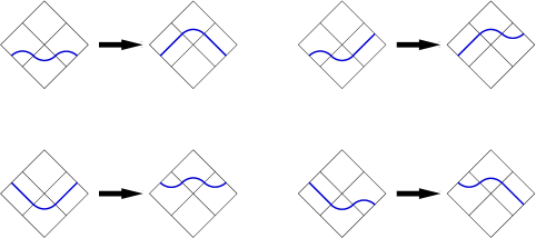
Figure 1: Drawings of how the intersection line (thick blue) must change how it crosses the diamonds (bordered in black) as it moves forward in time (upward on the page) over some small part of the loop worldsheet.

We have the general form of the metric perturbation (and its derivatives) for the four crossing types from Ref. Wachter and Olum (2017), and thus the general form of the accelerations for each source diamond. These expressions are analytic; in Appendix A we integrate them with respect to $u$ or $v$ to find the contribution of any source diamond to the tangent vector correction from the parameters of the source and observer diamonds, plus the range in $u$ or $v$ along the observer diamond’s line of motion for which the source diamond contributes. The above procedure for evolving the intersection line gives us all of this information.

Once we have found the tangent vector corrections, we have one more step before we may construct the new worldsheet. Consider a particular segment of $B$, with tangent vector

$$B^{\prime(0)}=\left(1\,,\,\mathbf{B}^{\prime(0)}\right)$$ (4)

applying over parameter range $\delta\sigma$. The correction, given by $\Delta B^{\prime}$, allows us to define a perturbed tangent vector $B^{\prime(1)}=B^{\prime(0)}+\Delta B^{\prime}$. This vector is still null to first order, but generally no longer has unit time component. Consequently, where we previously had $\tau=t$, this is no longer true (and, similarly, $\sigma$ no longer parameterizes energy). So, we use the correction to the time component of $B^{\prime}$ to reparameterize $\sigma$, defining a new null vector

$$\bar{B}^{\prime(1)}=\frac{B^{\prime(1)}}{1+\Delta B^{\prime t}}=\left(1\,,\,\frac{\mathbf{B}^{\prime(1)}}{1+\Delta B^{\prime t}}\right)\,.$$ (5)

Whereas before we had $B^{\prime(0)}=dB^{(0)}/d\sigma$, this new null vector obeys $\bar{B}^{\prime(1)}=dB^{(1)}/d\bar{\sigma}$, where $\bar{\sigma}$ is a reparameterization of $\sigma$ which depends on the correction. The old time component of $B^{(0)}$ ranged over an interval of length $\delta\sigma$, and the new time component of $B^{(1)}$ ranges over $\delta\bar{\sigma}$, so

$$\delta\bar{\sigma}=(1+\Delta B^{\prime t})\delta\sigma\,.$$ (6)

Usually $\Delta B^{\prime t}<0$, so $\delta\bar{\sigma}<\delta\sigma$, representing a loss of energy in backreaction.

The spatial part of Eq. (5) gives the new point on the unit sphere for this segment, and Eq. (6) gives its new length. We remove the overbars, and this reparameterized $\sigma$ once again represents the energy of the loop. By fixing $t$, we may create snapshots of the loop at a particular time Quashnock and Spergel (1990).

The procedure for any segment of $A$ is analogous, with the note that $A^{\prime}=-dA/d\sigma$.

II.3 Testing our approach

Before proceeding to our results, let us apply our approach to a well-studied case and verify that we recover the expected (analytical) result. To do this, we will consider the Garfinkle-Vachaspati class of degenerate loops Garfinkle and Vachaspati (1987), whose worldsheet functions are lines which go straight out and back in space and have some angle $\theta$ between them. The resulting loop is planar (and thus pathological), and the loop frozen at any point in its oscillation is a rectangle (including the degenerate double line cases).

The energy radiated in one oscillation for these loops can be found by taking the average gravitational radiation power from Ref. Garfinkle and Vachaspati (1987) and multiplying by the oscillation period, $L/2$. Dividing by the initial loop energy, $\mu L$ gives the fractional loss of length in one oscillation,

$$\frac{\Delta L}{L}=\frac{16G\mu}{\sin^{2}\theta}\left[(1+\cos\theta)\ln\left(\frac{2}{1+\cos\theta}\right)+(1-\cos\theta)\ln\left(\frac{2}{1-\cos\theta}\right)\right]\,.$$ (7)

For our test, we will perform gravitational backreaction on the Garfinkle-Vachaspati loops with $\theta=\{\pi/2,\pi/3,\pi/4,\pi/5\}$, and at each $\theta$ for $\{100,200,300,400\}$ segments in each of $A$ and $B$, for a single oscillation. Then we will determine the fraction of length lost by these loops using the numerical code that computes the backreaction and divide them by the expected analytic value. The plots of these results are in Fig. 2. Because our code accumulates the effect of backreaction over one oscillation before changing the loop, the loss of length it predicts for a pristine Garfinkle-Vachaspati loop should be exactly that of Eq. (7). We can therefore compare the numerical result, from the first oscillation only, to the analytic prediction above.

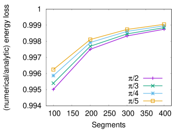
Figure 2: The numerical energy loss to gravitational radiation for a single oscillation of the Garfinkle-Vachaspati loop depends on the number of segments in the worldsheet functions $A$ and $B$. The value reported is the ratio of the numerical result to its analytically predicted result. As the number of segments increases, the ratio asymptotes towards unity, with the numerical result being within $\sim 0.1\%$ of the analytical result when there are $400$ segments in each of $A$ and $B$. We consider four different values for the angle between $A$ and $B$, but find that this does not greatly impact the accuracy of the result.

In all cases, we see that as the number of segments increases, the accuracy of our calculation improves. By the time we are at $400$ segments in each of $A$ and $B$, all results are within about $0.1\%$ of the analytic value.

III Results for simple models

We now present our results for the simple models which we studied. We defer detailed interpretation and discussion of these results to Sec. IV.

III.1 Simulation parameters

For all the loops studied in this section, we kept certain simulation parameters constant. First, we discretized all loops with $400$ segments in each of $A$ and $B$, yielding $160,000$ diamonds for the section of the worldsheet that includes a complete oscillation of a loop. We gave all segments the same initial length, because the $A^{\prime\prime}$ and $B^{\prime\prime}$ of the loops studied have almost (for $B$, exactly) the same magnitude everywhere. In general, when discretizing $A$ and $B$, one should put in more segments where the rates of change of the tangent vectors are higher, but this is not a concern until they are much higher at one place than at another.

Second, we evolved all loops for $200$ iterations with a step of $NG\mu=10^{-4}$ per iteration. These values were chosen so that by the end of the evolution, the loops would be roughly halfway dissipated, per the following. The energy lost per oscillation of the loop to gravitational radiation is Vilenkin and Shellard (2000)

$$\Delta E=\Gamma G\mu^{2}\left(\frac{L}{2}\right)\,,$$ (8)

where $\Gamma$ is a dimensionless constant that depends only on the loop’s geometry. The fraction of the loop which has dissipated after some number of iterations $n$ is then roughly

$$f_{\text{diss}}\sim\frac{n\Gamma NG\mu}{2}\,.$$ (9)

We pick $\Gamma=50$ because the distribution of $\Gamma$ for smoothed loops from simulations has a strong peak at this value Blanco-Pillado et al. (2015). With the choices above, we then obtain $f_{\text{diss}}\sim 1/2$, which means that in our simulations we will follow the loops for roughly half of their lifetimes. This is only a rough approximation because the actual $\Gamma$ may not be $50$, we have neglected the fact that the loop oscillates more rapidly as it loses energy, and $\Gamma$ itself will change due to backreaction. This final effect is discussed in more detail in Sec. IV.3.

Finally, we give all loops an initial length of $2\pi$ in arbitrary length units.

III.2 Model loops

Our goal in this paper is to simulate loops with cusps and loops with kinks (and some with both) to see how these features evolve. We need to start with loops that have no self intersections or other pathological features.

We start with a loop with cusps. The simplest such loop would be the 1,1 Burden Burden (1985) loop, whose $A$ and $B$ are just circles. However, this loop collapses into a double line. To prevent that, we perturb $A$ with a third-harmonic term, giving the Kibble-Turok loop Kibble and Turok (1982)

$$\mathbf{A}^{\prime}(v) =\left[(1-\alpha)\cos(v)+\alpha\cos(3v)\right]\,\hat{x}+\left[(1-\alpha)\sin(v)+\alpha\sin(3v)\right]\,\hat{y}$$

$$\qquad+2\sqrt{\alpha(1-\alpha)}\sin(v)\,\hat{z}\,,$$ (10a)

$$\mathbf{B}^{\prime}(u) =\cos(u)\,\hat{x}+\sin(u)\left(\cos\phi\,\hat{y}+\sin\phi\,\hat{z}\right)\,,$$ (10b)

where $\alpha\in(0,1)$ gives the magnitude of the perturbation and $\phi$ sets the angle between the planes of the tangent vectors before perturbation. This loop has no self intersections, and for $\alpha<\sin^{2}(\phi/2)$, it has two cusps. We will choose the parameters $\phi=\pi/2$ and $\alpha=0.1$. Our results are qualitatively unchanged by some variation in these values, but for $\alpha$ much smaller the loop is nearly self intersecting and for $\alpha$ much larger it has a very different character from the original Burden loop.

As this is the loop that we will then modify to produce the other loops, we refer to it as the canonical Kibble-Turok loop. Our motivation for studying this loop is to examine how cusps change as a result of backreaction.

Any loop with cusps may be converted into one with kinks by identifying where on the unit sphere the tangent vectors $\mathbf{A}^{\prime}$ and $\mathbf{B}^{\prime}$ overlap, then removing some of $\mathbf{A}^{\prime}$ and/or $\mathbf{B}^{\prime}$ around the cusp location (and reparameterizing the worldsheet functions so as to not change the overall length). For each such surgery performed, we introduce a kink.

We will construct our second loop by removing angle $\pi/2$ in two places from the path of $\mathbf{B}^{\prime}$ in the canonical Kibble-Turok loop, so that $\mathbf{B}^{\prime}$ skips over $\mathbf{A}^{\prime}$ instead of intersecting. Thus we replace two cusps with two kinks. (We could vary the amount of angle removed, but the results are qualitatively similar.) The expression for $\mathbf{A}^{\prime}$ is unchanged, but now we replace $u$ by $\tilde{u}$ in our expression for $\mathbf{B}^{\prime}$, where

$$\tilde{u}=\left\{\begin{array}[]{ll}(2u/L)(\pi-\psi)+\psi/2\,,&0<u\leq L/2\\ (2u/L)(\pi-\psi)+3\psi/2\,,&L/2<u\leq L\end{array}\right.\,.$$ (11)

We will call this the broken Kibble-Turok loop. Our motivation for studying it is to examine the ways in which kink evolution under backreaction differs from cusp evolution under backreaction.

Our third loop is the twice-broken Kibble-Turok loop. Now, we remove wedges of angle $\pi/2$ from both $\mathbf{A}^{\prime}$ and $\mathbf{B}^{\prime}$ around each cusp point. Again the tangent vectors no longer intersect on the unit sphere, but now we have replaced the two cusps with four kinks. Our motivation for studying this loop is that the scenario in which both tangent vectors jump over the same point is one generic to realistic loops. Such structures form from self-intersections, such as when the loops are produced from long strings or existing loops.

Our fourth and final loop is the cuspy broken Kibble-Turok loop. Here, $\mathbf{A}^{\prime}$ is untouched and $\mathbf{B}^{\prime}$ is broken, but the jump in the latter does not avoid the crossing with $\mathbf{A}^{\prime}$. This loop therefore has two cusps and two kinks. Our motivation for studying it is to see if the existence of cusps influences the evolution of kinks, and vice versa.

For brevity’s sake, we will refer to these four loops, in the order presented above, as the canonical, broken, twice-broken, and cuspy broken loops.

III.3 Canonical Kibble-Turok results

We present the basic results for the canonical loop in Figs. 3 and 4.

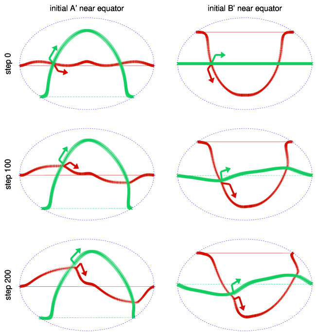
Figure 3: The motion of $\mathbf{A}^{\prime}$ (red, $+$) and $\mathbf{B}^{\prime}$ (green, $\times$) of the canonical loop about the unit sphere as a consequence of gravitational backreaction. The rows are, top to bottom, $0$, $100$ and $200$ iterations. In the left column we have chosen the projection so that the initial $\mathbf{A}^{\prime}$ lies mostly on the equator, and in the right columns so that the initial $\mathbf{B}^{\prime}$ lies on the equator. The three pictures in each column use the same projection. The two pictures in each row show the same data with different projections. Arrows show the location of segment 0 and the directions in which $u$ and $v$ increase (i.e., the directions of $\mathbf{A}^{\prime\prime}$ and $\mathbf{B}^{\prime\prime}$). Note that the cusps are “dragged” about the unit sphere.

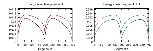
Figure 4: The energy per segment for the canonical loop worldsheet functions changing as a consequence of gravitational backreaction. We have plotted the energies for $0$, $100$ and $200$ iterations, with higher iterations having lower energies/darker colors. The energy loss is preferentially around the cusps and is of the same order on both sides.

Similar plots for the other scenarios will follow in later sections. To show how the tangent vectors evolve under gravitational backreaction, we plot $\mathbf{A}^{\prime}$ and $\mathbf{B}^{\prime}$ on the unit sphere under the Mollweide projection in Fig. 3. The left panels have $\mathbf{A}^{\prime}$ set to lie mostly on the equator, while the right panels do the same for $\mathbf{B}^{\prime}$. This is because the Mollweide projection is less distorted around the equator, and so using both projections lets us better understand how each of the tangent vectors change, and thus how kinks and cusps evolve. We show iterations $0$, $100$, and $200$, with the last corresponding to a loop of roughly half its initial length.

The most striking effect we see in Fig. 3 is that the cusp locations are dragged about the unit sphere. The segments of $\mathbf{A}^{\prime}$ and $\mathbf{B}^{\prime}$ are rotated, primarily in direction of $\mathbf{X}^{\prime\prime}=(\mathbf{A}^{\prime\prime}+\mathbf{B}^{\prime\prime})/2$. This moves the point of the cusp in that direction. It also moves the individual segments, so that the part of the string involved in successive cusps changes very little.

To show how energy is lost due to gravitational backreaction, we plot the length of all of the segments of both $A$ and $B$ for the same three iterations as before in Fig. 4. This allows us to see which parts of the string lose more energy during the backreaction process. The energy loss is preferentially around the cusp locations in both $A$ and $B$. In Fig. 5,

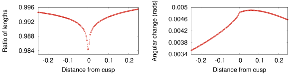
Figure 5: The change of the $2\%$ of overall points in $A$ nearest to the cusp due to the first iteration of backreaction. The length loss (left) is divergent and mostly symmetric, while the angular change (right) is bounded and is greater above the cusp (at $v>v_{\text{cusp}}$).

we look closely at the loss of energy near the cusp in just one iteration. It appears to be symmetrical and to diverge as the cusp is reached. Refs. Blanco-Pillado et al. (2018b); Chernoff et al. (2018) predicted a logarithmic divergence in the energy emission. The total acceleration felt by any worldsheet point which is not at the cusp goes as the inverse of the distance to the cusp, and integrating along a line on the worldsheet gives the logarithm. Following Sec. V of Ref. Blanco-Pillado et al. (2018b), working in the approximation that we are very near the cusp, we can analytically compute the effect of each source point, and numerically integrate to obtain the acceleration on each observation point. To compare this result to the acceleration reported by our code, we take a canonical loop and discretize it to $5\cdot 10^{5}$ diamonds, draw a straight line on the worldsheet which passes through the cusp, and find the acceleration at points along this line. This comparison is shown in Fig. 6,

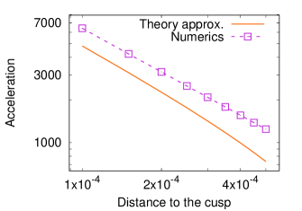
Figure 6: The comparison of numerics to the theoretical approximation near the cusp on the canonical loop. The theoretical and numerical accelerations both go like the inverse of the distance to the cusp. The theoretical approximation gets closer and closer to the numerical value as the observation point approaches the cusp. For numerical reasons we have not been able to get closer than about $10^{-4}L$.

where we see that the two approaches are converging up until a distance from the cusp of $\approx 10^{-4}L$. This is as close as we can get because of numerical errors, presumably arising from the high Lorentz factors of the segments near the cusp.

III.4 Broken Kibble-Turok results

We present the results for the broken loop in Figs. 7 and 8. Now, the cusps have been removed and replaced by kinks by removing sections of $B$ around the cusps, but keeping the overall length of $B$ the same.

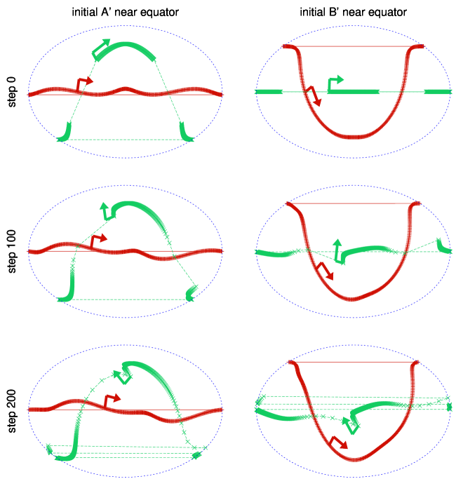
Figure 7: The motion of $\mathbf{A}^{\prime}$ (red, $+$) and $\mathbf{B}^{\prime}$ (green, $\times$) of the broken loop about the unit sphere.

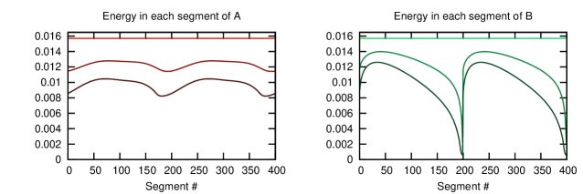
Figure 8: The energy per segment for the broken loop worldsheet functions changing as a consequence of gravitational backreaction. The energy loss is preferentially around the kinks in $B$ and is greater on the side with lower null parameter, while the energy loss in $A$ is less, but happens preferentially around where $B$ jumps over $A$.

There is still a preferential loss of energy around the place where the cusp would be — the “jumping-over point” — for both $A$ and $B$. However, it is much more pronounced in $B$. Closer examination in Fig. 9

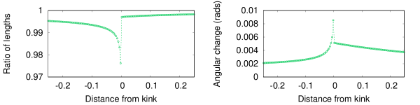
Figure 9: The change of the $2\%$ of overall points in $B$ on both sides of the kink due to one iteration of backreaction. The changes in both length and angle are asymmetric, being divergent below the kink and bounded above.

shows that the corrections to the energy and direction of the string diverge as $u$ approaches the kink position $u_{k}$ from below, but not when $u$ approaches $u_{k}$ from above. This divergent behavior was predicted in Refs. Blanco-Pillado et al. (2018b); Chernoff et al. (2018).

From Eq. (71) of Ref. Blanco-Pillado et al. (2018b), we can calculate analytically the acceleration felt by a point below a kink. We work to leading order as we approach the kink, meaning that we include only the term that diverges as $(u_{k}-u)^{-1/3}$ and not a subleading logarithmic divergence that was predicted but not calculated in Refs. Blanco-Pillado et al. (2018b); Chernoff et al. (2018). To compare the theoretical approximation to the value reported by our code, we take a broken loop and discretize it to $5\cdot 10^{5}$ diamonds, fix the $v$ index at some arbitrary value, and calculate the transverse acceleration for varying $u$ index values from a diamond far below the kink up to the diamond just below the kink. We plot these results in Fig. 10.

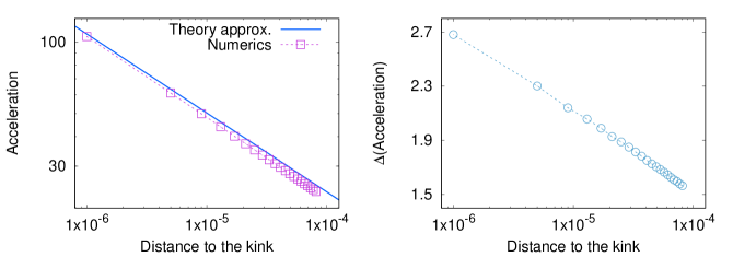
Figure 10: The comparison of numerics to theory for the broken loop. Left panel: The theoretical and numerical accelerations both go like the inverse cube root of the distance to the kink. Right panel: the difference between the theoretical and numerical accelerations goes like the logarithm of the distance to the kink. This is the lower-order divergent effect predicted in Ref. Blanco-Pillado et al. (2018b).

As the distance to the kink goes to zero, the leading effect in the numerical acceleration is the predicted $(u_{k}-u)^{-1/3}$ divergence, and the coefficient agrees with the theoretical prediction. The difference between the numerical and theoretical results shows the additional effect logarithmic in the distance to the kink.

Is it possible that this divergence could be an artifact, rather than a real, physical effect? First of all, it cannot be an artifact of the choice of spacetime gauge, because the perturbation of the spacetime metric around Minkowski space is always of order $G\mu$ and does not grow with time, while the effect of the gravitational backreaction on the string shape has secular growth. It also is not an artifact of the worldsheet gauge, i.e. the choice of the parameters $\tau$ and $\sigma$. These can be chosen to satisfy the conformal gauge conditions, thus defining the functions $A(v)$ and $B(u)$ and their tangent vectors $A^{\prime}$ and $B^{\prime}$, from which we see that $B^{\prime}$ has rapid variation over a small range of $u$. Finally, the rapid change in $B^{\prime}$ is not an artifact of which $B^{\prime}$ at later times we compare with which $B^{\prime}$ at earlier times. The directions in which $B^{\prime}$ points after backreaction are novel: no element of $B^{\prime}$ pointed close to these directions before, so we can see that these changes are large in a real sense and do not depend on any gauge or parameter choices.

How does this divergent correction arise? While there is no divergence in the metric perturbation at a point near the kink, there is a divergence in the derivatives in the null direction of the kink’s propagation (i.e., in $v$ for a kink in $B$). This divergence is as the inverse cube root of the null distance from the observation point to the kink (i.e., as $(u_{k}-u)^{-1/3}$ for a kink in $B$), which explains why we see a divergence in $B$ but not $A$ for the broken case. The divergence is integrable, so when we integrate the acceleration with respect to $u$ to find $\Delta A^{\prime}$, it becomes a finite correction. But to find $\Delta B^{\prime}$ we integrate with respect to $v$. Instead of crossing the kink as we integrate and thus removing the divergence, we travel around the worldsheet parallel to the kink, and so the divergence persists. However, as with the cusps, the total correction to the worldsheet ($\Delta A$ or $\Delta B$) will always be non-divergent regardless of which worldsheet function contains the kink, as finding these corrections requires integrating with respect to both $u$ and $v$.

As discussed in Ref. Blanco-Pillado et al. (2018b), the correction to $B$ diverges as one approaches the kink from one side. The kink will be rounded off by backreaction, and so we expect cusps to form. This is not the same, however, as the cusps which form due to the toy model of backreaction of Ref. Blanco-Pillado et al. (2015). There, the authors smoothed the string by convolving the functions $A^{\prime}$ and $B^{\prime}$ with a Lorentzian, which replaces a sharp kink by a smooth curve. For the rounding off discussed here, as can be seen in Figs. 7 and 8, the curvature happens over a very short amount of length (due to the energy near the kink being preferentially depleted). The effect seen here leads to a much higher $A^{\prime\prime}$ or $B^{\prime\prime}$ over a much shorter range compared to the convolution procedure of Ref. Blanco-Pillado et al. (2015). The cusps which actually form due to backreaction will therefore be weaker than previously predicted.

In the canonical loop, we expect the preferential loss of energy around the cusp to lead to the weakening of cusps. For the broken loop, we anticipate backreaction to lead to the formation of cusps, but because the string has already lost a good amount of energy modifying the kinks, the created cusps will be very weak.

III.5 Twice-broken Kibble-Turok results

We present the results for the twice-broken loop in Figs. 11 and 12.

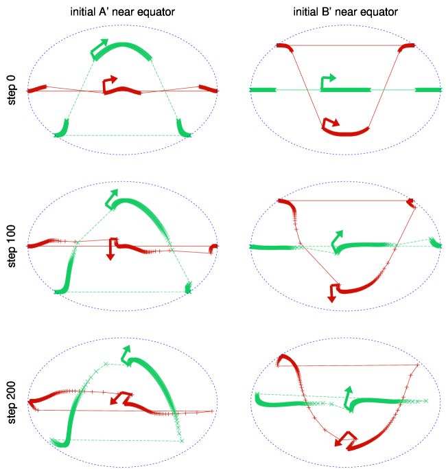
Figure 11: The motion of $\mathbf{A}^{\prime}$ (red, $+$) and $\mathbf{B}^{\prime}$ (green, $\times$) of the twice-broken loop about the unit sphere.

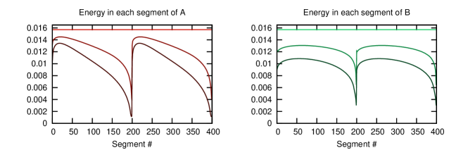
Figure 12: The energy per segment for the twice-broken loop worldsheet functions changing as a consequence of gravitational backreaction. The energy loss is preferentially around the kinks and is greater on the side with lower null parameter.

As with the broken loop, we see a preferential loss of energy for the segments around the kinks, although now it affects both $A$ and $B$ because both contain kinks. We moreover see the same change to the kinks as observed in the singly-broken case, both in rounding and in dragging.

III.6 Cuspy broken Kibble-Turok results

Lastly, we present the results for the cuspy broken loop in Figs. 13 and 14.

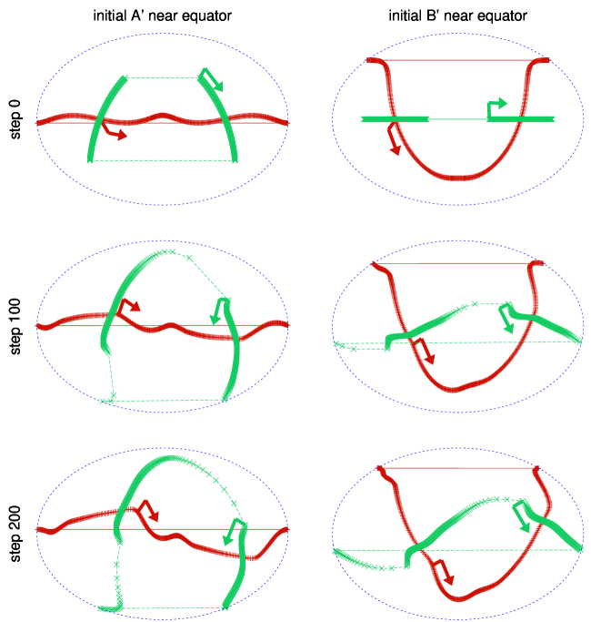
Figure 13: The motion of $\mathbf{A}^{\prime}$ (red, $+$) and $\mathbf{B}^{\prime}$ (green, $\times$) of the cuspy broken loop about the unit sphere.

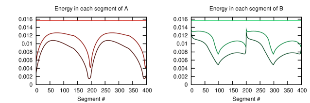
Figure 14: The energy per segment for the cuspy broken loop worldsheet functions changing as a consequence of gravitational backreaction. The energy loss is preferentially around the kinks and cusps; in the former case, the loss is greater on the side which has lower null parameter. The cusps are near segment $200$ and $400$ for $A$, and $100$ and $300$ for $B$. The kinks are shifted by $100$ segments from the cusps for both $A$ and $B$.

Now, we see that the preferential loss of energy at the kinks and cusps happens at slightly different rates, and with quite different behaviors. The depletion of energy and curving of the string near the kink happens preferentially on one side, whereas the depletion and curving near the cusp happen with roughly the same magnitude on both sides (although the process is not symmetric). Both the cusps and the kinks are dragged around the unit sphere, with the kinks being dragged faster.

The changes to the cusps and kinks in the cuspy broken case appear to be non-interfering, or at most weakly interfering. By this we mean that the cuspy broken loop behaves more or less like the superposition of the canonical and broken loops. This suggests that cusps and kinks only significantly change parts of the string very close to them, and also that the evolution of the kink does not depend strongly on whether or not it is avoiding a cusp.

IV General behavior under backreaction

IV.1 Changes to cusps

The locations of the cusps on the unit sphere are changed, in a process we have referred to as dragging. So, each time the cusp reappears, the direction in which it points is slightly different. This behavior was noted in Ref. Quashnock and Spergel (1990), where the cusps were said to be delayed. For example, in Fig. 3 we can clearly see that $\mathbf{A}^{\prime}$ is dragged in the direction of $\mathbf{B}^{\prime\prime}$, and looking closer we see that $\mathbf{B}^{\prime}$ is dragged in the direction of $\mathbf{A}^{\prime\prime}$ also. When we decide to describe the string in terms of $A$ and $B$ there is an arbitrary choice of the direction of $\sigma$, which determines which is $A$ and which is $B$, and similarly which is $u$ and which is $v$. It does not, however, affect the direction of advance of $u$ and $v$, because this is always toward the future. Thus the directions of the derivatives of $A$ and $B$ are not reversed. Since the dragging effect is symmetrical under exchange of $A$ and $B$, it does not depend on the choice of direction of $\sigma$.

The energy removed from the string by backreaction is preferentially taken from the string around the cusps, which leads to the cusps becoming weaker. The angular power density due to a cusp diverges as one approaches the cusp direction, but the total power radiated is finite. We model the cusp by expanding the string near the cusp in a Taylor series and following Appendix A of Ref. Blanco-Pillado and Olum (2017). Let us define $\Gamma_{\text{cusp}}(\theta)$ as the contribution to $\Gamma$ coming from radiation into the cone of directions within angle $\theta\ll 1$ of the cusp direction. We compute this quantity in Appendix B below. We find that $\Gamma_{\text{cusp}}(\theta)$ is proportional to $\theta$, so $\Gamma_{\text{cusp}}(\theta)/\theta$ does not depend on $\theta$ and characterizes the strength of the cusp. In Fig. 15,

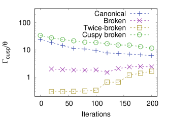
Figure 15: The changes in cusp strength (see text) due to gravitational backreaction.

we plot this strength as a function of the amount of backreaction.

Our measure, $\Gamma_{\text{cusp}}(\theta)/\theta$, is based on average power due to the cusp, not the energy of each burst. If a loop were to shrink without changing shape, this quantity would be constant. We found this measure useful for understanding changes in loop shape, but if you are interested in the observability of bursts, you should multiply by $L/2$ to get the burst energy per unit $\theta$. That measure would see an additional drop in energy due to the shrinkage of the loop.

Cusps which are initially present weaken over time, with the contribution to $\Gamma$ after iteration 200 being roughly half of what it was initially. The cuspy broken loop has a stronger cusp than the canonical loop, but this is due to how we constructed the loops. Recall that all loops start with the same length. Thus the wedge removed from the cuspy broken loop’s $B^{\prime}$ means that the same amount of energy as in the canonical case is spread across less angular distance, and thus the $\mathbf{B}^{\prime\prime}$ at the cusp is smaller in the cuspy broken case, so the radiation is stronger.

Cusps that develop on loops which lacked them initially start out weak and never grow as strong as the cusps that were there from the beginning. In the case of the broken loop, backreaction on the kink produces a somewhat smooth segment of $\mathbf{B}^{\prime}$ that crosses the pre-existing smooth $\mathbf{A}^{\prime}$ to form a cusp. In the case of the twice-broken loop, both $\mathbf{A}^{\prime}$ and $\mathbf{B}^{\prime}$ start with kinks. Thus in this case there is initially much less string involved in the cusp (i.e., both $\mathbf{A}^{\prime\prime}$ and $\mathbf{B}^{\prime\prime}$ are much larger), and thus the cusp radiation is much weaker than in the singly-broken case.

Since the weak cusps are getting stronger and the strong cusps weaker, there may be a convergence to a single strength of cusps in all cases, but it is hard to tell. Even if so, such a thing would happen only after most of the loop’s energy has been lost.

IV.2 Changes to kinks

The locations of the kinks on the unit sphere are dragged, again in the general direction of $\mathbf{X}^{\prime\prime}$. As far as we know this behavior has not been discussed before. We cannot comment extensively on the relative rates of cusp and kink dragging, but they appear to differ by less than an order of magnitude.

The energy removed from the string by backreaction is also preferentially taken from the string around the kinks — more strongly for whichever of $A$ or $B$ contains the discontinuity, but both are affected. While the cusps lose energy roughly equally on both sides, the kinks lose energy in a very asymmetric fashion, with the side above the kink being almost unaffected and the side below being quickly depleted Blanco-Pillado et al. (2018b).

The kink is rounded off, also in an asymmetrical fashion, as we see, for example, in Fig. 7. In the bottom panels, several of the original segments now fill the gap seen in the top panels. However, we also see from Fig. 8 that little of the energy associated with each of these segments still remains. Thus backreaction replaces the kink by a curved section, but this curvature is confined to a quite small region of the string. While the kink has been rounded off, and so is no longer completely preventing cusps, any cusps which do form will be weak compared to the cusps we studied which were present at a loop’s creation. We can see this behavior in Fig. 15.

IV.3 Changes in $\Gamma$

In Fig. 16,

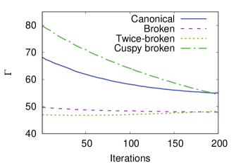
Figure 16: The changes in loop $\Gamma$ due to gravitational backreaction.

we show the evolution of the $\Gamma$ factors for all loops discussed above. Loops that start with cusps have higher $\Gamma$, which is not surprising. Such loops preferentially lose energy from the region around the cusp. This leads to a decline in the cusp radiation and contributes to a decline in the overall $\Gamma$.

Loops without cusps initially start with lower $\Gamma$, and there is little change in $\Gamma$ over time. Backreaction introduces cusps, but the emission from them is always weaker than that of cusps present initially. The production of cusps does not increase the overall $\Gamma$, so the (fairly small) emission from the cusps must be offset by decreases in emission elsewhere.

We further observe that the changes to the $\Gamma$ values is in a rough correspondence to the changes to the cusp strengths seen in Fig. 15.

In the end, all loops appear to evolve towards a $\Gamma$ in the high $40$s or low $50$s, although there does not appear to be a single asymptotic value. This is similar to the $\Gamma\approx 50$ for loops taken from simulations and smoothed Blanco-Pillado et al. (2015), although this does not explain why a simple model loop would move towards a configuration similar to a loop generated by a stochastic process.

Note that the change in $\Gamma$ is due to a change in the shape of the string, and not to its decreasing length. This change in shape should also change the power spectrum, $P_{n}$, of the string, particularly in the high-$n$ regime where the difference between kinks and cusps dominates.

IV.4 Self-Intersections

One of the important questions one would like to address is how robust non-self-intersecting trajectories are to the effects of backreaction. This was studied in detail for realistic loops obtained from a large scale simulation in Blanco-Pillado et al. (2015) using a toy model for backreaction based on smoothing. This led to the conclusion that backreaction usually did not deform non-self-intersecting loops into self-intersecting trajectories. Here we revisit this issue, but with explicit backreaction in place of a toy model.

We check for self-intersections by taking the backreacted loops at various points in their evolution and letting them undergo one full oscillation in flat space. During this motion, we are sensitive to any crossing of segments, which would lead to the loop fragmenting into two child loops. We have not found any such self-intersections in these cases. This seems to be the generic situation for this family of loops.

V Conclusions

We have developed and demonstrated a technique for calculating gravitational backreaction on cosmic string loops, although we have only studied simple models in this work. This was done in order to draw conclusions on the fates of cusps and kinks in as controlled of an environment as possible. However, we are currently studying backreaction on realistic cosmic string loops, as will be reported in a future paper.

As expected from analytic work Blanco-Pillado et al. (2018b), backreaction acting on one side of a kink rounds it off immediately, but only over a narrow region of the string. Viewed very close up, the string is smooth, but at larger distances it still looks like a kink. Smoothing produces a cusp that was not there initially, but this cusp is very weak, and never grows very strong as compared to what one would expect for a loop whose $\mathbf{A}^{\prime}$ and $\mathbf{B}^{\prime}$ move uniformly around the unit sphere.

There are two reasons that cusps never grow very strong. First, the amount of the initial string involved in the rounding of the kink grows only slowly with time. But secondly, the energy in this string is always being depleted, so that even as more and more of the initial segments of string are involved in the cusp, the amount of energy in each segment is going down.

For strings with cusps initially, the amount of energy involved in the cusp, and consequently the cusp strength, declines over time by a factor of a few by the time the loop is about half evaporated.

Loops produced in simulations have many kinks, but no cusps Blanco-Pillado et al. (2015), because the paths of $\mathbf{A}^{\prime}$ and $\mathbf{B}^{\prime}$ often jump over each other but never cross smoothly. Thus we expect the results on the initially cuspless loops that we study in this paper to be the ones relevant for prediction of observable signals from a cosmic string network. These cusps never grow to more than about one-tenth of the naive cusp strength that one would predict for a smooth loop. This worsens the prospects for detection of burst signals, such as gravitational waves, coming from cusps, and thus weakens the constraints from non-detection.

Cusps are “dragged” about the unit sphere in the general direction of $\mathbf{X}^{\prime\prime}$. Thus successive bursts of gravitational waves from cusps are emitted in slightly different directions, so one would not expect observations of repeating bursts. Figure 17 shows the angular distance on the unit sphere between the direction of each cusp and where it was originally.

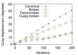
Figure 17: Motion of the cusp direction around the unit sphere due to backreaction.

In roughly the first half of the loop lifetime, studied here, the angles are no more than $50^{\circ}$. This has some impact on the rocket effect Vachaspati and Vilenkin (1985); Durrer (1989) because the thrust due to gravitational wave emission is not in a single direction, but it is tiny. For $\theta=50^{\circ}$, the average thrust is only reduced 3% over what it would be without dragging.

Finally, we note that describing the effect of backreaction on a loop is not as simple as saying that cusps are weakened and kinks are rounded off. These processes indeed take place, but parts of the loop far from kinks or cusps are also affected, in complex ways. In particular we see that the dragging process affects segments near kinks or cusps more than those further away, introducing features that were not originally present. The resulting loops are not simply described as having, or not having, cusps and kinks.

Appendix A Corrections to a segment due to a single source diamond

Given an observer diamond and a source diamond on some string worldsheet, we may find the correction to the observer $A^{\prime}$ and $B^{\prime}$ due to that source. To do this, we make use of the $uvcd$ coordinates of Ref. Blanco-Pillado et al. (2018b). These are pseudo-orthonormal coordinates whose basis vectors are $B^{\prime}/2$ for the $u$ direction and $A^{\prime}/2$ for the $v$ direction, using the null vectors of the source, plus two spacelike vectors for the $c$ and $d$ direction which are orthogonal to the plane of the source diamond and to each other. Thus the source diamond is parameterized by the null parameters $u$ and $v$. This also means that

$$A^{\prime\gamma} =(0,2,0,0)\,,$$ (12a)

$$B^{\prime\gamma} =(2,0,0,0)$$ (12b)

when $\gamma=(u,v,c,d)$.

Some additional definitions will make the following equations more compact. First we say that the observer’s motion in the observer diamond is along the null vector $V$, parameterized by $x$. Thus, if $\kappa$ connects the centers of the source and observer diamonds, then we can define

$$\Omega(x)=\kappa+\frac{xV}{2}$$ (13)

as the location of the observer relative to the source diamond’s center, which we take as the origin of our coordinate system. The edges of the source diamond have length $L_{A}$ and $L_{B}$, and so locally $u$ runs over $-L_{B}\ldots L_{B}$, and similarly for $v$ and $L_{A}$. This means that we can define vectors

$$E =\Omega-L_{A}A^{\prime}/2-L_{B}B^{\prime}/2\,,$$ (14a)

$$S =\Omega+L_{A}A^{\prime}/2+L_{B}B^{\prime}/2\,,$$ (14b)

which point from the future tip and past tip of the source diamond, respectively, to the observer. We also define $Z=A^{\prime}\cdot B^{\prime}$ for convenience, and indicate the null vectors of the observer diamond by $\bar{A}^{\prime}$ and $\bar{B}^{\prime}$ to distinguish them from the source diamond null vectors. Finally, we use the freedom in $c$ and $d$ to choose our coordinates such that $V^{d}=0$ always.

We will now take Eq. (19) of Ref. Wachter and Olum (2017),

$$h_{\alpha\beta}=\frac{8G\mu\sigma_{\alpha\beta}}{Z}\ln\left[\frac{2A^{\prime}\Omega}{Z}-u\right]^{u_{+}}_{u_{-}}\,,$$ (15)

with $h_{\alpha\beta}$ the first-order perturbation of the spacetime metric due to the source diamond,

$$\sigma_{\alpha\beta}=\frac{1}{2}\left(A^{\prime}_{\alpha}B^{\prime}_{\beta}+B^{\prime}_{\alpha}A^{\prime}_{\beta}-4Z\eta_{\alpha\beta}\right)\,,$$ (16)

$\eta_{\alpha\beta}$ the flat-space metric, and $u_{\pm}$ the maximum and minimum values of that parameter visited by the intersection line within the source diamond. Then, making use of Eqs. (1,3), we find that the correction to a null vector $\bar{N}^{\prime}$ of the observer diamond due to the source diamond is given by

$$\Delta\bar{N}^{\lambda} =-G\mu\left[\left(\bar{A}^{\prime v}A^{\prime\lambda}+\bar{A}^{\prime u}B^{\prime\lambda}-2\bar{A}^{\prime\lambda}\right)F_{\rho}\bar{B}^{\prime\rho}+\left(\bar{B}^{\prime v}A^{\prime\lambda}+\bar{B}^{\prime u}B^{\prime\lambda}-2\bar{B}^{\prime\lambda}\right)F_{\rho}\bar{A}^{\prime\rho}\right.$$

$$\qquad\qquad\left.+F^{\lambda}\left(\bar{A}^{\prime c}\bar{B}^{\prime c}+\bar{A}^{\prime d}\bar{B}^{\prime d}\right)\right]\,,$$ (17)

where $F$ is given by

$$\int^{x_{f}}_{x_{i}}h_{\alpha\beta,\gamma}=\frac{8G\mu\sigma_{\alpha\beta}}{Z}F_{\gamma}\,.$$ (18)

The values of $F_{\gamma}$ depend on which of the three types of crossing discussed in Sec. II.2 the source diamond possesses. This crossing type may change as we move along the observer line in the observer diamond, and thus a single source diamond could contribute up to three separate $\Delta\bar{N}^{\prime}$ terms which correct the observer diamond’s null vector. The initial and final values of the null parameter we integrate over, $x_{i}$ and $x_{f}$, give the range of the observer’s motion for a given crossing type.

For an intersection line which connects opposite edges of fixed $u$,

$$F_{u} =\frac{2}{V^{u}}\left(\ln\left[\frac{E^{u}(x_{f})}{E^{u}(x_{i})}\right]-\ln\left[\frac{S^{u}(x_{f})}{S^{u}(x_{i})}\right]\right)\,,$$ (19a)

$$F_{v} =0\,,$$ (19b)

$$F_{c} =0\,,$$ (19c)

$$F_{d} =0\,.$$ (19d)

For an intersection line which connects opposite edges of fixed $v$, the $F$ are the same as the case which connects edges of fixed $u$, but with $u\leftrightarrow v$. For an intersection line which connects the two future edges of the source diamond,

$$F_{u} =\frac{2}{V^{u}}\ln\left[\frac{E^{u}(x_{f})}{E^{u}(x_{i})}\right]\,,$$ (20a)

$$F_{v} =\frac{2}{V^{v}}\ln\left[\frac{E^{v}(x_{f})}{E^{v}(x_{i})}\right]\,,$$ (20b)

$$F_{c} =-\frac{2}{V^{c}}\ln\left[\frac{(\Omega^{c}(x_{f}))^{2}+(\Omega^{d})^{2}}{(\Omega^{c}(x_{i}))^{2}+(\Omega^{d})^{2}}\right]\,,$$ (20c)

$$F_{d} =-\frac{4}{V^{c}}\arctan\left[\frac{(\Omega^{c}(x_{f})-\Omega^{c}(x_{i}))\Omega^{d}}{(\Omega^{d})^{2}+\Omega^{c}(x_{f})\Omega^{c}(x_{i})}\right]\,.$$ (20d)

Note that because $V^{d}=0$, $\Omega^{d}$ has no dependence on $x$. Finally, for an intersection line which connects the two past edges of the source diamond, the $F$ are as the case which connects the two future edges, but with the overall sign of each $F$ changed and with $E\rightarrow S$.

With the forms of the $F$, and Eq. (12), we may simplify Eq. (A). For a $u$-type crossing, we know that only $F_{u}\neq 0$, and so the velocity correction becomes

$$\Delta\bar{N}^{u} =0\,,$$ (21a)

$$\Delta\bar{N}^{v} =-\frac{G\mu F_{u}}{Z}\left(\bar{A}^{\prime c}\bar{B}^{\prime c}+\bar{A}^{\prime d}\bar{B}^{\prime d}\right)\,,$$ (21b)

$$\Delta\bar{N}^{c} =G\mu F_{u}\left(\bar{B}^{\prime u}\bar{A}^{\prime c}+\bar{A}^{\prime u}\bar{B}^{\prime c}\right)\,,$$ (21c)

$$\Delta\bar{N}^{d} =G\mu F_{u}\left(\bar{B}^{\prime u}\bar{A}^{\prime d}+\bar{A}^{\prime u}\bar{B}^{\prime d}\right)\,.$$ (21d)

For a $v$-type crossing, by the usual symmetry of $u\leftrightarrow v$ and $A^{\prime}\leftrightarrow B^{\prime}$, we find

$$\Delta\bar{N}^{u} =-\frac{G\mu F_{v}}{Z}\left(\bar{A}^{\prime c}\bar{B}^{\prime c}+\bar{A}^{\prime d}\bar{B}^{\prime d}\right)\,,$$ (22a)

$$\Delta\bar{N}^{v} =0\,,$$ (22b)

$$\Delta\bar{N}^{c} =G\mu F_{v}\left(\bar{B}^{\prime v}\bar{A}^{\prime c}+\bar{A}^{\prime v}\bar{B}^{\prime c}\right)\,,$$ (22c)

$$\Delta\bar{N}^{d} =G\mu F_{v}\left(\bar{B}^{\prime v}\bar{A}^{\prime d}+\bar{A}^{\prime v}\bar{B}^{\prime d}\right)\,.$$ (22d)

For a past- or future-type crossing, no member of $F_{\gamma}$ is generally zero. So,

$$\Delta\bar{N}^{u} =-\frac{G\mu F_{v}}{Z}\left(\bar{A}^{\prime c}\bar{B}^{\prime c}+\bar{A}^{\prime d}\bar{B}^{\prime d}\right)\,,$$ (23a)

$$\Delta\bar{N}^{v} =-\frac{G\mu F_{u}}{Z}\left(\bar{A}^{\prime c}\bar{B}^{\prime c}+\bar{A}^{\prime d}\bar{B}^{\prime d}\right)\,,$$ (23b)

$$\Delta\bar{N}^{c} =G\mu\bar{A}^{\prime c}F_{\rho}\bar{B}^{\prime\rho}+G\mu\bar{B}^{\prime c}F_{\rho}\bar{A}^{\prime\rho}-G\mu F_{c}\left(\bar{A}^{\prime c}\bar{B}^{\prime c}+\bar{A}^{\prime d}\bar{B}^{\prime d}\right)\,,$$ (23c)

$$\Delta\bar{N}^{d} =G\mu\bar{A}^{\prime d}F_{\rho}\bar{B}^{\prime\rho}+G\mu\bar{B}^{\prime d}F_{\rho}\bar{A}^{\prime\rho}-G\mu F_{d}\left(\bar{A}^{\prime c}\bar{B}^{\prime c}+\bar{A}^{\prime d}\bar{B}^{\prime d}\right)\,,$$ (23d)

with the difference in the two crossing types coming entirely from the $F_{\gamma}$ terms.

Appendix B Calculating $\Gamma_{\text{cusp}}$

The angular power density in gravitational waves emitted by a cusp diverges as the observer approaches the cusp direction. We would like to use the coefficient of this divergence to characterize the strength of the cusp.

We begin by considering a coordinate system oriented so that $\mathbf{A}^{\prime}=\mathbf{B}^{\prime}$ points entirely in the $z$ direction, so $\mathbf{A}^{\prime\prime}$ and $\mathbf{B}^{\prime\prime}$ lie entirely in the $x$-$y$ plane. We establish spherical polar coordinates $(\theta,\phi)$, where $\theta=0$ is the cusp direction. Let $(\theta_{O},\phi_{O})$ denote the direction of the observer in these coordinates. We consider directions close to the cusp, $\theta_{O}\ll 1$. The directions of $\mathbf{A}^{\prime\prime}$ and $\mathbf{B}^{\prime\prime}$ are $(\pi/2,\phi_{A})$ and $(\pi/2,\phi_{B})$ respectively. Define the relative angles $\phi_{AO}=\phi_{A}-\phi_{O}$ and $\phi_{BO}=\phi_{B}-\phi_{O}$, and $\phi_{AB}=\phi_{A}-\phi_{B}$.

The power per unit frequency $\omega$ per unit solid angle is given by Eq. (A29) of Ref. Blanco-Pillado and Olum (2017),

$$\frac{dP}{d\omega d\Omega}= \frac{2G\mu^{2}\omega^{2}\theta_{O}^{8}}{9\pi^{2}L}\frac{\sin^{4}\phi_{AO}\sin^{4}\phi_{BO}}{|\mathbf{A}^{\prime\prime}|^{2}|\mathbf{B}^{\prime\prime}|^{2}}\left[(K^{2}_{1/3}(\xi_{A})+K^{2}_{2/3}(\xi_{A}))(K^{2}_{1/3}(\xi_{B})+K^{2}_{2/3}(\xi_{B}))\right.$$

$$\left.+4\operatorname{sign}(\sin\phi_{AO}\sin\phi_{BO})K_{1/3}(\xi_{A})K_{2/3}(\xi_{A})K_{1/3}(\xi_{B})K_{2/3}(\xi_{B})\right]\,.$$ (24)

Here $K_{\alpha}$ is the modified Bessel function of the second kind, and we have defined

$$\xi_{A}=\omega\theta_{O}^{3}\frac{|\sin^{3}\phi_{AO}|}{6|\mathbf{A}^{\prime\prime}|}$$ (25)

and likewise for $\xi_{B}$.

We change variables from $\omega$ to

$$w=\sqrt{\frac{|\sin^{3}\phi_{AO}\sin^{3}\phi_{BO}|}{36|\mathbf{A}^{\prime\prime}||\mathbf{B}^{\prime\prime}|}}\theta_{O}^{3}\omega$$ (26)

and integrate over $w$ to get

$$\frac{dP}{d\Omega}=\frac{48G\mu^{2}}{\theta_{O}\pi^{2}L}\frac{1}{(|\mathbf{A}^{\prime\prime}||\mathbf{B}^{\prime\prime}||\sin\phi_{AO}\sin\phi_{BO}|)^{1/2}}\mathcal{H}_{\operatorname{sign}(\sin\phi_{AO}\sin\phi_{BO})}(a)\,,$$ (27)

where

$$a=\frac{\xi_{A}}{\xi_{B}}=\frac{|\mathbf{B}^{\prime\prime}|}{|\mathbf{A}^{\prime\prime}|}\left|\frac{\sin\phi_{AO}}{\sin\phi_{BO}}\right|^{3}$$ (28)

and

$$\mathcal{H}_{\pm}(a)=\int^{\infty}_{0}w^{2} \left[(K^{2}_{1/3}(a^{-1/2}w)+K^{2}_{2/3}(a^{-1/2}w))(K^{2}_{1/3}(a^{1/2}w)+K^{2}_{2/3}(a^{1/2}w))\right.$$

$$\left.\pm 4K_{1/3}(a^{-1/2}w)K_{2/3}(a^{-1/2}w)K_{1/3}(a^{1/2}w)K_{2/3}(a^{1/2}w)\right]dw\,.$$ (29)

This is invariant under $a\rightarrow 1/a$, and thus Eq. (27) is invariant under the interchange of $A$ and $B$. It is also invariant under rescalings of the loop length, as both $|\mathbf{A}^{\prime\prime}|$ and $|\mathbf{B}^{\prime\prime}|$ go like $1/L$. Length-invariance makes this quantity a good measure of cusp strength for considering how backreaction changes a cusp on a loop over time, as the loop’s length is also changing due to backreaction.

In the main text we defined $\Gamma_{\text{cusp}}(\theta)$ to be the contribution to $\Gamma$ coming from angles within $\theta$ of the cusp direction. So we should compute

$$\int_{0}^{2\pi}d\phi_{O}\int_{0}^{\theta}\sin\theta_{O}\,d\theta_{O}\,\frac{dP}{d\Omega}$$ (30)

and then use $P=G\mu^{2}\Gamma$ to find the contribution to $\Gamma$. The polar integration is straightforward, because we are working in the regime where $\theta_{O}\ll 1$ and thus $\sin\theta_{O}\approx\theta_{O}$. The $\theta_{O}$ here cancels the $\theta_{O}$ in the denominator of Eq. (27), and so our expression is overall $\propto\theta$. Due to the dependence of $a$ and $w$ on $\phi_{O}$, the azimuthal integration must be done numerically. This integration gives some number $\Gamma_{\text{cusp}}/\theta$, which we show in Fig. 15.

References

- Kibble (1976) T. W. B. Kibble, “Topology of Cosmic Domains and Strings,” J. Phys. A9, 1387–1398 (1976).
- Vilenkin and Shellard (2000) A. Vilenkin and E. P. S. Shellard, Cosmic Strings and Other Topological Defects (Cambridge University Press, 2000).
- Jeannerot et al. (2003) Rachel Jeannerot, Jonathan Rocher, and Mairi Sakellariadou, “How generic is cosmic string formation in SUSY GUTs,” Phys. Rev. D68, 103514 (2003), arXiv:hep-ph/0308134 [hep-ph] .
- Sarangi and Tye (2002) Saswat Sarangi and S. H. Henry Tye, “Cosmic string production towards the end of brane inflation,” Phys. Lett. B536, 185–192 (2002), arXiv:hep-th/0204074 [hep-th] .
- Dvali and Vilenkin (2004) Gia Dvali and Alexander Vilenkin, “Formation and evolution of cosmic D strings,” JCAP 0403, 010 (2004), arXiv:hep-th/0312007 [hep-th] .
- Copeland et al. (2004) Edmund J. Copeland, Robert C. Myers, and Joseph Polchinski, “Cosmic F and D strings,” JHEP 06, 013 (2004), arXiv:hep-th/0312067 [hep-th] .
- Vilenkin (1981) A. Vilenkin, “Gravitational radiation from cosmic strings,” Phys. Lett. 107B, 47–50 (1981).
- Hogan and Rees (1984) C. J. Hogan and M. J. Rees, “Gravitational interactions of cosmic strings,” Nature 311, 109–113 (1984), [,128(1984)].
- Vachaspati and Vilenkin (1985) Tanmay Vachaspati and Alexander Vilenkin, “Gravitational Radiation from Cosmic Strings,” Phys. Rev. D31, 3052 (1985).
- Accetta and Krauss (1989) Frank S. Accetta and Lawrence M. Krauss, “The stochastic gravitational wave spectrum resulting from cosmic string evolution,” Nucl. Phys. B319, 747–764 (1989).
- Bennett and Bouchet (1991) David P. Bennett and Francois R. Bouchet, “Constraints on the gravity wave background generated by cosmic strings,” Phys. Rev. D43, 2733–2735 (1991).
- Caldwell and Allen (1992) R. R. Caldwell and Bruce Allen, “Cosmological constraints on cosmic string gravitational radiation,” Phys. Rev. D45, 3447–3468 (1992).
- Damour and Vilenkin (2000) Thibault Damour and Alexander Vilenkin, “Gravitational wave bursts from cosmic strings,” Phys. Rev. Lett. 85, 3761–3764 (2000), arXiv:gr-qc/0004075 [gr-qc] .
- Damour and Vilenkin (2001) Thibault Damour and Alexander Vilenkin, “Gravitational wave bursts from cusps and kinks on cosmic strings,” Phys. Rev. D64, 064008 (2001), arXiv:gr-qc/0104026 [gr-qc] .
- Damour and Vilenkin (2005) Thibault Damour and Alexander Vilenkin, “Gravitational radiation from cosmic (super)strings: Bursts, stochastic background, and observational windows,” Phys. Rev. D71, 063510 (2005), arXiv:hep-th/0410222 [hep-th] .
- Siemens et al. (2007) Xavier Siemens, Vuk Mandic, and Jolien Creighton, “Gravitational wave stochastic background from cosmic (super)strings,” Phys. Rev. Lett. 98, 111101 (2007), arXiv:astro-ph/0610920 [astro-ph] .
- DePies and Hogan (2007) Matthew R. DePies and Craig J. Hogan, “Stochastic Gravitational Wave Background from Light Cosmic Strings,” Phys. Rev. D75, 125006 (2007), arXiv:astro-ph/0702335 [astro-ph] .
- Olmez et al. (2010) S. Olmez, V. Mandic, and X. Siemens, “Gravitational-Wave Stochastic Background from Kinks and Cusps on Cosmic Strings,” Phys. Rev. D81, 104028 (2010), arXiv:1004.0890 [astro-ph.CO] .
- Sanidas et al. (2012) S. A. Sanidas, R. A. Battye, and B. W. Stappers, “Constraints on cosmic string tension imposed by the limit on the stochastic gravitational wave background from the European Pulsar Timing Array,” Phys. Rev. D85, 122003 (2012), arXiv:1201.2419 [astro-ph.CO] .
- Sanidas et al. (2013) Sotirios A. Sanidas, Richard A. Battye, and Benjamin W. Stappers, “Projected constraints on the cosmic (super)string tension with future gravitational wave detection experiments,” Astrophys. J. 764, 108 (2013), arXiv:1211.5042 [astro-ph.CO] .
- Binetruy et al. (2012) Pierre Binetruy, Alejandro Bohe, Chiara Caprini, and Jean-Francois Dufaux, “Cosmological Backgrounds of Gravitational Waves and eLISA/NGO: Phase Transitions, Cosmic Strings and Other Sources,” JCAP 1206, 027 (2012), arXiv:1201.0983 [gr-qc] .
- Kuroyanagi et al. (2012) Sachiko Kuroyanagi, Koichi Miyamoto, Toyokazu Sekiguchi, Keitaro Takahashi, and Joseph Silk, “Forecast constraints on cosmic string parameters from gravitational wave direct detection experiments,” Phys. Rev. D86, 023503 (2012), arXiv:1202.3032 [astro-ph.CO] .
- Blanco-Pillado et al. (2014) Jose J. Blanco-Pillado, Ken D. Olum, and Benjamin Shlaer, “The number of cosmic string loops,” Phys. Rev. D89, 023512 (2014), arXiv:1309.6637 [astro-ph.CO] .
- Sousa and Avelino (2016) L. Sousa and P. P. Avelino, “Probing Cosmic Superstrings with Gravitational Waves,” Phys. Rev. D94, 063529 (2016), arXiv:1606.05585 [astro-ph.CO] .
- Blanco-Pillado and Olum (2017) Jose J. Blanco-Pillado and Ken D. Olum, “Stochastic gravitational wave background from smoothed cosmic string loops,” Phys. Rev. D96, 104046 (2017), arXiv:1709.02693 [astro-ph.CO] .
- Blanco-Pillado et al. (2018a) Jose J. Blanco-Pillado, Ken D. Olum, and Xavier Siemens, “New limits on cosmic strings from gravitational wave observation,” Phys. Lett. B778, 392–396 (2018a), arXiv:1709.02434 [astro-ph.CO] .
- Cui et al. (2018) Yanou Cui, Marek Lewicki, David E. Morrissey, and James D. Wells, “Cosmic Archaeology with Gravitational Waves from Cosmic Strings,” Phys. Rev. D97, 123505 (2018), arXiv:1711.03104 [hep-ph] .
- Chernoff and Tye (2018) David F. Chernoff and S. H. Henry Tye, “Detection of Low Tension Cosmic Superstrings,” JCAP 1805, 002 (2018), arXiv:1712.05060 [astro-ph.CO] .
- Ringeval and Suyama (2017) Christophe Ringeval and Teruaki Suyama, “Stochastic gravitational waves from cosmic string loops in scaling,” JCAP 1712, 027 (2017), arXiv:1709.03845 [astro-ph.CO] .
- Guedes et al. (2018) G. S. F. Guedes, P. P. Avelino, and L. Sousa, “Signature of inflation in the stochastic gravitational wave background generated by cosmic string networks,” Phys. Rev. D98, 123505 (2018), arXiv:1809.10802 [astro-ph.CO] .
- Abbott et al. (2016) B. P. Abbott et al. (LIGO Scientific, Virgo), “Search for transient gravitational waves in coincidence with short-duration radio transients during 2007–2013,” Phys. Rev. D93, 122008 (2016), arXiv:1605.01707 [astro-ph.HE] .
- Herner et al. (2017) K. Herner et al., “Optical Follow-up of Gravitational Wave Triggers with DECam,” Proceedings, 22nd International Conference on Computing in High Energy and Nuclear Physics (CHEP2016): San Francisco, CA, October 14-16, 2016, J. Phys. Conf. Ser. 898, 032050 (2017).
- Abbott et al. (2018) B. P. Abbott et al. (LIGO Scientific, Virgo), “Constraints on cosmic strings using data from the first Advanced LIGO observing run,” Phys. Rev. D97, 102002 (2018), arXiv:1712.01168 [gr-qc] .
- Quashnock and Spergel (1990) Jean M. Quashnock and David N. Spergel, “Gravitational Selfinteractions of Cosmic Strings,” Phys. Rev. D42, 2505–2520 (1990).
- Blanco-Pillado et al. (2018b) Jose J. Blanco-Pillado, Ken D. Olum, and Jeremy M. Wachter, “Gravitational backreaction near cosmic string kinks and cusps,” Phys. Rev. D98, 123507 (2018b), arXiv:1808.08254 [gr-qc] .
- Chernoff et al. (2018) David F. Chernoff, Éanna É. Flanagan, and Barry Wardell, “Gravitational backreaction on a cosmic string: Formalism,” (2018), arXiv:1808.08631 [gr-qc] .
- Wachter and Olum (2017) Jeremy M. Wachter and Ken D. Olum, “Gravitational backreaction on piecewise linear cosmic string loops,” Phys. Rev. D95, 023519 (2017), arXiv:1609.01685 [gr-qc] .
- Blanco-Pillado et al. (2015) Jose J. Blanco-Pillado, Ken D. Olum, and Benjamin Shlaer, “Cosmic string loop shapes,” Phys. Rev. D92, 063528 (2015), arXiv:1508.02693 [astro-ph.CO] .
- Blanco-Pillado et al. (2011) Jose J. Blanco-Pillado, Ken D. Olum, and Benjamin Shlaer, “Large parallel cosmic string simulations: New results on loop production,” Phys. Rev. D83, 083514 (2011), arXiv:1101.5173 [astro-ph.CO] .
- Garfinkle and Vachaspati (1987) David Garfinkle and Tanmay Vachaspati, “Radiation From Kinky, Cuspless Cosmic Loops,” Phys. Rev. D36, 2229 (1987).
- Kibble and Turok (1982) T. W. B. Kibble and Neil Turok, “Selfintersection of Cosmic Strings,” Phys. Lett. 116B, 141–143 (1982).
- Burden (1985) C. J. Burden, “Gravitational Radiation From a Particular Class of Cosmic Strings,” Phys. Lett. 164B, 277–281 (1985).
- Durrer (1989) R. Durrer, “Gravitational Angular Momentum Radiation of Cosmic Strings,” Nucl. Phys. B328, 238–271 (1989).