Splitting of the homology of the punctured mapping class group

Abstract.

Let $\Gamma_{g,1}^{m}$ be the mapping class group of the orientable surface $\Sigma_{g,1}^{m}$ of genus $g$ with one parametrised boundary curve and $m$ permutable punctures; when $m=0$ we omit it from the notation. Let $\beta_{m}(\Sigma_{g,1})$ be the braid group on $m$ strands of the surface $\Sigma_{g,1}$.

We prove that $H_{*}(\Gamma_{g,1}^{m};\mathbb{Z}_{2})\cong H_{*}(\Gamma_{g,1};H_{*}(\beta_{m}(\Sigma_{g,1});\mathbb{Z}_{2}))$. The main ingredient is the computation of $H_{*}(\beta_{m}(\Sigma_{g,1});\mathbb{Z}_{2})$ as a symplectic representation of $\Gamma_{g,1}$.

1. Introduction

Let $\Sigma_{g,1}$ be a smooth orientable surface of genus $g$ with one boundary curve $\partial\Sigma_{g,1}$, and let $\Sigma_{g,1}^{m}$ be $\Sigma_{g,1}$ with a choice of $m$ distinct points in the interior, called punctures.

Let $\Gamma_{g,1}$ be the mapping class group of $\Sigma_{g,1}$, i.e. the group of isotopy classes of diffeomorphisms of $\Sigma_{g,1}$: diffeomorphisms are required to fix $\partial\Sigma_{g,1}$ pointwise. Similarly let $\Gamma_{g,1}^{m}$ be the mapping class group of $\Sigma_{g,1}^{m}$, i.e. the group of isotopy classes of diffeomorphisms of $\Sigma_{g,1}^{m}$ that fix $\partial\Sigma_{g,1}^{m}$ pointwise and permute the $m$ punctures.

Forgetting the punctures gives a surjective map $\Gamma_{g,1}^{m}\to\Gamma_{g,1}$ with kernel $\beta_{m}(\Sigma_{g,1})$, the $m$-th braid group of the surface $\Sigma_{g,1}$. We obtain the Birman exact sequence (see [1])

(1) $$1\to\beta_{m}(\Sigma_{g,1})\to\Gamma_{g,1}^{m}\to\Gamma_{g,1}\to 1.$$

The associated Leray-Serre spectral sequence $E(m)$ in $\mathbb{Z}_{2}$-homology has a second page $E(m)^{2}_{k,q}=H_{k}(\Gamma_{g,1};H_{q}(\beta_{m}(\Sigma_{g,1});\mathbb{Z}_{2}))$, and converges to $H_{k+q}(\Gamma_{g,1}^{m};\mathbb{Z}_{2})$.

The main result of this article is that this spectral sequence collapses in its second page.

Theorem 1.1.

For all $l\geq 0$ there is an isomorphism of vector spaces

(2) $$H_{l}\left(\Gamma_{g,1}^{m};\mathbb{Z}_{2}\right)\cong\bigoplus_{k+q=l}H_{k}\left(\Gamma_{g,1};H_{q}\left(\beta_{m}(\Sigma_{g,1});\mathbb{Z}_{2}\right)\right).$$

Thus the computation of $H_{*}\left(\Gamma_{g,1}^{m};\mathbb{Z}_{2}\right)$ reduces to the computation of the homology of $\Gamma_{g,1}$ with twisted coefficients in the representation $H_{*}\left(\beta_{m}(\Sigma_{g,1});\mathbb{Z}_{2}\right)$. We will see that this $\Gamma_{g,1}$-representation splits as a direct sum of symmetric powers of $H_{1}(\Sigma_{g,1})$ with the symplectic action: this is done in Theorem 3.2, which together with Theorem 1.1 is the main result of the article.

The strategy of the proof does not generalize to fields of characteristic different from 2 or to the pure mapping class group, in which we consider only diffeomorphisms of $\Sigma_{g,1}^{m}$ that fix all punctures. In Section 7 we describe in detail a counterexample with coefficients in $\mathbb{Q}$, which can be generalized both to coefficients in a field $\mathbb{F}_{p}$ of odd characteristic and to the pure mapping class group.

I would like to thank my PhD advisor Carl-Friedrich Bödigheimer for his precious suggestions and his continuous encouragement during the preparation of this work.

2. Preliminaries

In the whole article $\mathbb{Z}_{2}$-coefficients for homology and cohomology will be understood, unless explicitly stated otherwise.

In this section we recollect some classical definitions and results about braid groups and mapping class groups.

Definition 2.1.

The $m$-th ordered configuration space of a surface $\Sigma_{g,1}$ is the space

$$F_{m}(\Sigma_{g,1})=\left\{(P_{1},\dots,P_{m})\in\left(\mathring{\Sigma}_{g,1}\right)^{\times m}\,|\,P_{i}\neq P_{j}\;\forall i\neq j\right\}.$$

Note that we require the points of the configuration to lie in the interior of $\Sigma_{g,1}$; the space $F_{m}(\Sigma_{g,1})$ is a smooth, orientable $2m$-dimensional manifold.

The symmetric group $\mathfrak{S}_{m}$ acts freely on $F_{m}(\Sigma_{g,1})$ by permuting the labels $1,\dots,m$ of a configuration; the orbit space

$$F_{m}(\Sigma_{g,1})/\mathfrak{S}_{m}$$

is called the $m$-th unordered configuration space of $\Sigma_{g,1}$ and is denoted by $C_{m}(\Sigma_{g,1})$; this space is also a $2m$-dimensional orientable manifold (see Figure 1).

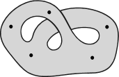
Figure 1. A configuration in the space $C_{5}(\Sigma_{1,1})$

A classical result by Fadell and Neuwirth ([8]) ensures that $C_{m}(\Sigma_{g,1})$ is aspherical; the fundamental group $\pi_{1}(C_{m}(\Sigma_{g,1}))$ is called the braid group on $m$ strands of $\Sigma_{g,1}$ and is denoted by $\beta_{m}(\Sigma_{g,1})$.

Definition 2.2.

Let $\operatorname{Diff}(\Sigma_{g,1};\partial\Sigma_{g,1})$ be the group of diffeomorphisms of $\Sigma_{g,1}$ that fix $\partial\Sigma_{g,1}$ pointwise, endowed with the Whitney $C^{\infty}$-topology. We denote by $\Gamma_{g,1}=\pi_{0}(\operatorname{Diff}(\Sigma_{g,1};\partial\Sigma_{g,1}))$ its group of connected components, which is called the mapping class group of $\Sigma_{g,1}$.

Similarly let $\operatorname{Diff}(\Sigma_{g,1}^{m};\partial\Sigma_{g,1}^{m})$ be the group of diffeomorphisms of $\Sigma_{g,1}^{m}$ that fix $\partial(\Sigma_{g,1})$ pointwise and restrict to a permutation of the $m$ punctures: the mapping class group of $\Sigma_{g,1}^{m}$ is $\Gamma_{g,1}^{m}=\pi_{0}(\operatorname{Diff}(\Sigma_{g,1}^{m};\partial\Sigma_{g,1}^{m}))$.

A classical result by Earle and Schatz [7] ensures that the connected components of $\operatorname{Diff}(\Sigma_{g,1};\partial\Sigma_{g,1})$ are contractible: note that for $g=0$ and $g=1$ this result holds because we consider surfaces with non-empty boundary, and the bounday must be fixed pointwise by our diffeomorphisms. In particular $B\operatorname{Diff}(\Sigma_{g,1};\partial\Sigma_{g,1})\simeq B\Gamma_{g,1}$ is a classifying space for the group $\Gamma_{g,1}$, i.e. an Eilenberg-MacLane space of type $K(\Gamma_{g,1},1)$.

We call $\mathcal{F}_{g,1}\to B\operatorname{Diff}(\Sigma_{g,1};\partial\Sigma_{g,1})$ the universal $\Sigma_{g,1}$-bundle

$$\Sigma_{g,1}\to\mathcal{F}_{g,1}=\Sigma_{g,1}\times_{\operatorname{Diff}(\Sigma_{g,1};\partial\Sigma_{g,1})}E\operatorname{Diff}(\Sigma_{g,1};\partial\Sigma_{g,1})\to B\operatorname{Diff}(\Sigma_{g,1};\partial\Sigma_{g,1}).$$

Applying the construction of the $m$-th unordered configuration space fiberwise we obtain a bundle $C_{m}(\mathcal{F}_{g,1})\to B\operatorname{Diff}(\Sigma_{g,1};\partial\Sigma_{g,1})$ with fiber $C_{m}(\Sigma_{g,1})$.

The space $C_{m}(\mathcal{F}_{g,1})$ is a classifying space for the group $\Gamma_{g,1}^{m}$ and the Birman exact sequence (1) is obtained by taking fundamental groups of the aspherical spaces

(3) $$C_{m}(\Sigma_{g,1})\to C_{m}(\mathcal{F}_{g,1})\to B\operatorname{Diff}(\Sigma_{g,1};\partial\Sigma_{g,1}).$$

In the whole article the genus $g\geq 0$ of the surfaces that we consider is supposed to be fixed, and we will abbreviate $\mathcal{S}=\Sigma_{g,1}$. We denote by $\mathcal{D}$ the open disc $\mathring{\Sigma}_{0,1}$.

It will be useful, for many constructions, to choose an embedding $\mathcal{D}\hookrightarrow\mathring{\mathcal{S}}$ near $\partial\mathcal{S}$ and to replace $\operatorname{Diff}(\mathcal{S};\partial\mathcal{S})$ with its subgroup $\operatorname{Diff}(\mathcal{S};\partial\mathcal{S}\cup\mathcal{D})$ of diffeomorphisms of $\mathcal{S}$ that fix pointwise both $\partial\mathcal{S}$ and $\mathcal{D}$. Saying that $\mathcal{D}$ is embedded near $\partial\mathcal{S}$ means that there is a compact subsurface $\mathcal{S}^{\prime}\subset\mathcal{S}$ such that $\mathcal{S}=\mathcal{S}^{\prime}\natural\bar{\mathcal{D}}$ is the union along a segment of $\mathcal{S}^{\prime}$ and the closure of $\mathcal{D}$ in $\mathcal{S}$.

From now on we suppose such an embedding to be fixed and we consider $\mathcal{D}$ as a subspace of $\mathring{\mathcal{S}}$ (see Figure 2). In Section 3, Definition 3.3, we will introduce a convenient model $\mathcal{T}(\mathcal{S})$ for the space $\mathring{\mathcal{S}}$, and in Section 4, Definition 4.1 we will specify an embedding $\mathcal{D}\hookrightarrow\mathring{\mathcal{S}}$ using the model $\mathcal{T}(\mathcal{S})$.

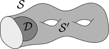
Figure 2. A splitting of $\mathcal{S}$ as $\mathcal{S}^{\prime}\natural\bar{\mathcal{D}}$.

The construction in Definition 2.1 can be specialised to the surfaces $\mathcal{D}$ and $\mathcal{S}^{\prime}$, yielding spaces $C_{m}(\mathcal{D})$ and $C_{m}(\mathcal{S}^{\prime})$ respectively. We take configurations of points in the interior of the surfaces $\mathcal{D}$ and $\mathcal{S}^{\prime}$ respectively (since $\mathcal{D}$ is already an open surface this remark applies in particular to $\mathcal{S}^{\prime}$).

The inclusion $\operatorname{Diff}(\mathcal{S};\partial\mathcal{S}\cup\mathcal{D})\subset\operatorname{Diff}(\mathcal{S};\partial\mathcal{S})$ is a homotopy equivalence of topological groups, hence also the induced map

$$B\operatorname{Diff}(\mathcal{S};\partial\mathcal{S}\cup\mathcal{D})\to B\operatorname{Diff}(\mathcal{S};\partial\mathcal{S})$$

is a homotopy equivalence. We will replace the previous construction with the following, homotopy equivalent ones.

Definition 2.3.

We call $\mathcal{F}_{\mathcal{S},\mathcal{D}}\to B\operatorname{Diff}(\mathcal{S};\partial\mathcal{S}\cup\mathcal{D})$ the universal $\mathcal{S}$-bundle

$$\mathcal{S}\to\mathcal{F}_{\mathcal{S},\mathcal{D}}\colon=\mathcal{S}\times_{\operatorname{Diff}(\mathcal{S};\partial\mathcal{S}\cup\mathcal{D})}E\operatorname{Diff}(\mathcal{S};\partial\mathcal{S}\cup\mathcal{D})\to B\operatorname{Diff}(\mathcal{S};\partial\mathcal{S}\cup\mathcal{D}).$$

Note that $\operatorname{Diff}(\mathcal{S};\partial\mathcal{S}\cup\mathcal{D})$ acts on $\mathcal{S}^{\prime}$ by restriction of diffeomorphisms, and acts trivially on $\mathcal{D}$; therefore $\mathcal{F}_{\mathcal{S},\mathcal{D}}$ contains subspaces

$$\mathcal{F}_{\mathcal{S}^{\prime}}=\mathcal{S}^{\prime}\times_{\operatorname{Diff}(\mathcal{S};\partial\mathcal{S}\cup\mathcal{D})}E\operatorname{Diff}(\mathcal{S};\partial\mathcal{S}\cup\mathcal{D})$$

and $\mathcal{D}\times B\operatorname{Diff}(\mathcal{S};\partial\mathcal{S}\cup\mathcal{D})$; these subspaces fiber over $B\operatorname{Diff}(\mathcal{S};\partial\mathcal{S}\cup\mathcal{D})$ with fibers $\mathcal{S}^{\prime}$ and $\mathcal{D}$ respectively.

Applying the construction of the $m$-th unordered configuration space fiberwise, we obtain spaces $C_{m}(\mathcal{F}_{\mathcal{S},\mathcal{D}})$, $C_{m}(\mathcal{F}_{\mathcal{S}^{\prime}})$ and $C_{m}(\mathcal{D})\times B\operatorname{Diff}(\mathcal{S};\partial\mathcal{S}\cup\mathcal{D})$, all fibering over $B\operatorname{Diff}(\mathcal{S};\partial\mathcal{S}\cup\mathcal{D})$, respectively with fiber $C_{m}(\mathcal{S})$, $C_{m}(\mathcal{S}^{\prime})$ and $C_{m}(\mathcal{D})$.

The fiber bundle (3) corresponding to the Birman exact sequence (1) can now be replaced with the following one

(4) $$C_{m}(\mathcal{S})\to C_{m}(\mathcal{F}_{\mathcal{S},\mathcal{D}})\to B\operatorname{Diff}(\mathcal{S};\partial\mathcal{S}\cup\mathcal{D}).$$

Definition 2.4.

For all $0\leq p\leq m$ there is a map

$$\mu\colon C_{p}(\mathcal{D})\times C_{m-p}(\mathcal{S}^{\prime})\to C_{m}(\mathcal{S})$$

which takes the union of configurations (see Figure 3):

$$\mu\left(\left\{P_{1},\dots,P_{p}\right\};\left\{P^{\prime}_{1},\dots,P^{\prime}_{m-p}\right\}\right)=\left\{P_{1},\dots,P_{p},P^{\prime}_{1},\dots,P^{\prime}_{m-p}\right\}\in C_{m}(\mathcal{S}).$$

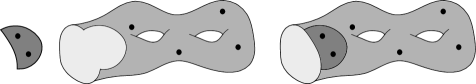
Figure 3. The product of two configurations in $C_{2}(\mathcal{D})$ and $C_{4}(\mathcal{S}^{\prime})$.

We can apply this construction at the same time to each couple of fibers of the bundles $C_{m}(\mathcal{F}_{\mathcal{S},\mathcal{D}})$ and $C_{m-p}(\mathcal{F}_{\mathcal{S}^{\prime}})$ lying over the same point of $B\operatorname{Diff}(\mathcal{S};\partial\mathcal{S}\cup\mathcal{D})$.

We obtain a map

$$\mu^{\mathcal{F}}\colon C_{p}(\mathcal{D})\times C_{m-p}(\mathcal{F}_{\mathcal{S}^{\prime}})\to C_{m}(\mathcal{F}_{\mathcal{S},\mathcal{D}}).$$

If we see the domain of $\mu^{\mathcal{F}}$ as a fibered product of bundles over $B\operatorname{Diff}(\mathcal{S};\partial\mathcal{S}\cup\mathcal{D})$

$$\left(C_{m}(\mathcal{D})\times B\operatorname{Diff}(\mathcal{S};\partial\mathcal{S}\cup\mathcal{D})\right)\times_{B\operatorname{Diff}(\mathcal{S};\partial\mathcal{S}\cup\mathcal{D})}C_{m-p}(\mathcal{F}_{\mathcal{S}^{\prime}}),$$

then the map $\mu^{\mathcal{F}}$ is also a map of bundles over $B\operatorname{Diff}(\mathcal{S};\partial\mathcal{S}\cup\mathcal{D})$, and the corresponding map on fibers is precisely $\mu$.

We recall now the structure of $H_{*}(C_{m}(\mathcal{D}))$. The cohomology of $C_{m}(\mathcal{D})$ with coefficients in $\mathbb{Z}_{2}$ was first computed by Fuchs in [9]: in section 3 we will generalise Fuchs’ argument to surfaces with boundary of positive genus.

In the appendix of [6, Chap.III], Cohen considers the space $\coprod_{m\geq 0}C_{m}(\mathcal{D})$ as an algebra over the operad of little $2$-cubes, and describes its $\mathbb{Z}_{2}$-homology as follows:

(5) $$H_{*}\left(\coprod_{m\geq 0}C_{m}(\mathcal{D})\right)\cong\mathbb{Z}_{2}\left[Q^{j}\varepsilon\,|\,j\geq 0\right].$$

Here $\varepsilon\in H_{0}(C_{1}(\mathcal{D}))$ is the fundamental class, and for all $k,m\geq 0$ we denote by $Q\colon H_{k}(C_{m}(\mathcal{D}))\to H_{2k+1}(C_{2m}(\mathcal{D}))$ the first Dyer-Lashof operation. In particular $Q^{j}\varepsilon$ is the generator of $H_{2^{j}-1}(C_{2^{j}}(\mathcal{D}))\simeq\mathbb{Z}_{2}$. See Figure 4.

The isomorphism in equation (5) is an isomorphism of bigraded rings. The left-hand side is a ring with the Pontryagin product, and the right-hand side is a polynomial ring in infinitely many variables $\varepsilon,Q\varepsilon,Q^{2}\varepsilon,\dots$. The bigrading is given by the homological degree $*$, that we call the degree, and by the index $m$ of the connected component on which the homology class is supported (informally, the number of points involved in the construction of the homology class), that we call the weight.

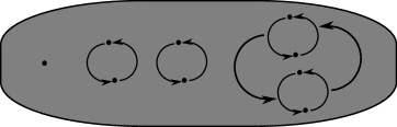
Figure 4. The class in $H_{5}(C_{9}(\mathcal{D}))$ corresponding to the monomial $\varepsilon\cdot(Q\varepsilon)^{2}\cdot Q^{2}\varepsilon$.

In this article we will only need the isomorphism in equation (5) to hold as an isomorphism of bigraded $\mathbb{Z}_{2}$-vector spaces. In particular for all choices of natural numbers $(\alpha_{j})_{j\geq 0}$ with all but finitely many $\alpha_{j}=0$, we will consider the monomial $\prod_{j}\left(Q^{j}\varepsilon\right)^{\alpha_{j}}$, corresponding to a homology class in some bigrading $(*,m)$: we will only use the fact that the set of these monomials is a bigraded basis for the left-hand side of equation (5).

We end this section recalling the classical notions of symmetric product and one-point compactification.

Definition 2.5.

The $m$-fold symmetric product of a topological space $\mathcal{M}$, denoted by $S\!P^{m}(\mathcal{M})$, is the quotient of $\mathcal{M}^{m}$ by the (non-free) action of the symmetric group $\mathfrak{S}_{m}$ which permutes the coordinates.

We regard a point of $S\!P^{m}(\mathcal{M})$ as a configuration of $m$ points in $\mathcal{M}$ with multiplicities.

In the case of an open surface $\mathring{\mathcal{S}}$, it is known that $S\!P^{m}(\mathring{\mathcal{S}})$ is a non-compact manifold of dimension $2m$; it contains $C_{m}(\mathcal{S})$ as an open submanifold.

Definition 2.6.

For a space $\mathcal{M}$ we denote by $\mathcal{M}^{\infty}$ its one-point compactification; the basepoint is the point at infinity, that we denote by $\infty$.

We will consider in particular the one-point-compactification $C_{m}(\mathcal{S})^{\infty}$ of $C_{m}(\mathcal{S})$.

3. Homology of configuration spaces of surfaces

We want to study $H_{*}(\beta_{m}(\Sigma_{g,1}))=H_{*}(C_{m}(\mathcal{S}))$, which appears as the homology of the fiber in the Leray-Serre spectral sequence associated to (1), (3) or (4). In particular we are interested in $H_{*}(C_{m}(\mathcal{S}))$ as a $\mathbb{Z}_{2}$-representation of the group $\Gamma_{g,1}$.

In [13] Löffler and Milgram implicitly proved that $H_{*}(\beta_{m}(\Sigma_{g,1}))=H_{*}(C_{m}(\mathcal{S}))$ is a $\mathbb{Z}_{2}$-symplectic representation of the mapping class group. By $\mathbb{Z}_{2}$-symplectic we mean the following:

Definition 3.1.

Let $\mathcal{H}=H_{1}(\mathcal{S})\simeq\mathbb{Z}_{2}^{2g}$. The natural action of $\Gamma_{g,1}$ on $\mathcal{H}$ induces a surjective map $\Gamma_{g,1}\to Sp_{2g}(\mathbb{Z}_{2})$. A representation of $\Gamma_{g,1}$ over $\mathbb{Z}_{2}$ is called $\mathbb{Z}_{2}$-symplectic if it is a pull-back of a representation of $Sp_{2g}(\mathbb{Z}_{2})$ along this map.

In [3] Bödigheimer, Cohen and Taylor computed $H_{*}(C_{m}(\mathcal{S}))$ as a graded $\mathbb{Z}_{2}$-vector space. Their method provides all Betti numbers, but the action of $\Gamma_{g,1}$ cannot be easily deduced: their descripition of $H_{*}(C_{m}(\mathcal{S}))$ depends on a handle decomposition of $\mathcal{S}$, which is not preserved by diffeomorphisms of $\mathcal{S}$, not even up to isotopy.

In this section and in the next one we will prove the following theorem; to the best of the author’s knowledge it does not appear in the literature.

Theorem 3.2.

There is an isomorphism of bigraded $\mathbb{Z}_{2}$-representations of $\Gamma_{g,1}$

$$\bigoplus_{m\geq 0}H_{*}\left(C_{m}(\mathcal{S})\right)\cong\mathbb{Z}_{2}\left[Q^{j}\varepsilon\,|\,j\geq 0\right]\otimes\operatorname{Sym}_{\bullet}(\mathcal{H}).$$

Here we mean the following:

• on the left-hand side the bigrading is given by homological degree $*$ and by the direct summand, indexed by $m$, on which the homology class is supported, i.e. by the number $m$ of points involved in constructing the homology class; we call $*$ the degree and $m$ the weight, and write $(*,m)$ for the bigrading;

• for $j\geq 0$, $Q^{j}\varepsilon$ is the image in $H_{2^{j}-1}(C_{2^{j}}(\mathcal{S}))$ of a generator of the group $H_{2^{j}-1}(C_{2^{j}}(\mathcal{D}))\simeq\mathbb{Z}_{2}$ under the natural map induced by the embedding $\mathcal{D}\hookrightarrow\mathring{\mathcal{S}}$, and $\mathbb{Z}_{2}\left[Q^{j}\varepsilon\,|\,j\geq 0\right]$ is the polynomial ring on infinitely many variables $\varepsilon,Q\varepsilon,Q^{2}\varepsilon,\dots$;

• $\mathcal{H}=H_{1}(\Sigma_{g,1})$ is identified with $H_{1}(C_{1}(\mathcal{S}))$ in a natural way, and lives in degree $1$ and weight $1$; $\operatorname{Sym}_{\bullet}(\mathcal{H})$ denotes the symmetric algebra on $\mathcal{H}$;

• degrees and weights are extended on the right-hand side by the usual multiplicativity rule;

• the action of $\Gamma_{g,1}$ on the right is the tensor product of the trivial action on the factor $\mathbb{Z}_{2}[Q^{j}\varepsilon\,|\,j\geq 0]$, and of the action on $\operatorname{Sym}_{\bullet}(\mathcal{H})$ which is induced by the $\mathbb{Z}_{2}$-symplectic action on $\mathcal{H}$.

Note that for any bi-homogeneus element in the right-hand side, the weight is greater or equal than the degree: indeed factors of the form $Q^{j}\varepsilon$ have weight strictly higher than their degree, whereas factors belonging to $\mathcal{H}$ or to its symmetric powers have equal weight and degree.

Note that in the case $g=0$ the group $\Gamma_{0,1}$ is trivial and the previous theorem reduces to equation (5).

We point out that in [4] Bödigheimer and Tillmann have essentially proved that for a field $\mathbb{F}$ of any characteristic the $\mathbb{F}$-vector space

$$\bigoplus_{m\geq 0}H_{*}\left(C_{m}(\mathcal{S});\mathbb{F}\right)$$

is isomorphic, as a bigraded $\Gamma_{g,1}$-representation over $\mathbb{F}$, to the tensor product of the ring $\mathbb{F}[\varepsilon]$, with trivial action, and some other bigraded representation: here $\varepsilon$ denotes, in analogy with the notation of Theorem 3.2, the standard generator of $H_{0}(C_{1}(\mathcal{D}))$. In Section 6 we will compare in detail Theorems 3.2 and 1.1 with the results in [4].

In this section we will prove that there is an isomorphism of bigraded $\mathbb{Z}_{2}$-vector spaces as in Theorem 3.2; in the next section we will deal with the action of $\Gamma_{g,1}$.

Since we work with coefficients in a field, it is equivalent to compute homology or cohomology, and in this section we will prefer to compute $H^{*}(C_{m}(\mathcal{S}))$ for all bigradings $(*,m)$.

We will mimic the method used by Fuchs [9] to compute the $\mathbb{Z}_{2}$-cohomology of $C_{m}(\mathcal{D})$. As already mentioned in Section 2, our computation recovers a known result, but it has the advantage of being quite elementary and of providing a part of the geometric insight that we will need in the next section.

In the whole section we assume $m\geq 0$ to be fixed. Since the space $C_{m}(\mathcal{S})$ is homeomorphic to the interior of a compact $2m$-manifold with boundary, by Poincaré-Lefschetz duality we have

$$H^{*}(C_{m}(\mathcal{S}))\simeq\tilde{H}_{2m-*}(C_{m}(\mathcal{S})^{\infty}),$$

where in the right hand side we consider reduced homology of the one-point compactification (see Definition 2.6).

We introduce a space $\mathcal{T}(\mathcal{S})$ which is homeomorphic to $\mathring{\mathcal{S}}$, the interior of $\mathcal{S}$. The construction corresponds to a handle decomposition of $\mathcal{S}$ with one $0$-handle and $2g$ $1$-handles.

Definition 3.3.

If $g=0$, hence $\mathcal{S}=\Sigma_{0,1}$ is the disc, we set $\mathcal{T}(\mathcal{S})=]0,1[^{2}$, the interior of the unit square. Assume now $g\geq 1$, and see Figure 5 to visualize the following construction.

Dissect the interval $[0,1]$ into $2g$ equal subintervals through the points $\mathcal{P}_{i}=\frac{i}{2g}$ for $0\leq i\leq 2g$ (for $i=0,2g$ we get the two endpoints of $[0,1]$).

Consider on the vertical sides of $[0,1]^{2}$ the intervals $I_{i}^{l}=\left\{0\right\}\times[\mathcal{P}_{i},\mathcal{P}_{i+1}]$ and $I_{i}^{r}=\left\{1\right\}\times[\mathcal{P}_{i},\mathcal{P}_{i+1}]$ for $1\leq i\leq 2g$: all these intervals are canonically diffeomorphic to $[0,1]$ by projecting on the second coordinate, rescaling linearly by a factor $2g$ and translating.

We define a bijection between the two sets of left and right intervals: for $1\leq i\leq g$, the interval $I^{l}_{2i-1}$ corresponds to $I^{r}_{2i}$, and the interval $I^{r}_{2i-1}$ corresponds $I^{l}_{2i}$.

The space $Q(\mathcal{S})$ is the quotient of the square $[0,1]^{2}$ obtained by identifying each couple of corresponding intervals in the canonical way. For $1\leq i\leq g$ we call $\overline{\mathcal{U}}_{i}$ the image of $I^{l}_{2i-1}$ in the quotient $Q(\mathcal{S})$, and we call $\overline{\mathcal{V}}_{i}$ the image of $I^{l}_{2g}$ in $Q(\mathcal{S})$.

Note that the image in $Q(\mathcal{S})$ of the set $\left\{0,1\right\}\times\left\{\mathcal{P}_{0},\dots,\mathcal{P}_{2g}\right\}$ consists of two points $\mathcal{P}_{odd}$ and $\mathcal{P}_{even}$: for $\varepsilon\in\left\{0,1\right\}$ and $0\leq i\leq 2g$ the point $(\varepsilon,\mathcal{P}_{i})$ is mapped to $\mathcal{P}_{even}$ if $\varepsilon+i$ is even, and is mapped to $\mathcal{P}_{odd}$ otherwise.

The spaces $\overline{\mathcal{U}}_{i}\subset Q(\mathcal{S})$ and $\overline{\mathcal{V}}_{i}\subset Q(\mathcal{S})$ are intervals with endpoints $\mathcal{P}_{even}$ and $\mathcal{P}_{odd}$; the interiors of these intervals are disjoint. Each $\overline{\mathcal{U}}_{i}$ and $\overline{\mathcal{V}}_{i}$ is the homeomorphic image of some left interval $I^{l}_{j}$, and inherits from the latter a parametrisation by $[0,1]$.

We call $\mathcal{U}_{i}$ and $\mathcal{V}_{i}$ the interiors of the intervals $\overline{\mathcal{U}}_{i}$ and $\overline{\mathcal{V}}_{i}$ respectively.

The space $Q(\mathcal{S})$ is homeomorphic to the compact surface $\mathcal{S}$; we call $\mathcal{T}(\mathcal{S})$ the interior of $Q(\mathcal{S})$.

From now on we will identify $\mathcal{S}$ with $Q(\mathcal{S})$ and $\mathring{\mathcal{S}}$ with $\mathcal{T}(\mathcal{S})$; consequently we will identify $C_{m}(\mathcal{S})$ with the space of configurations of $m$ points in $\mathcal{T}(\mathcal{S})$.

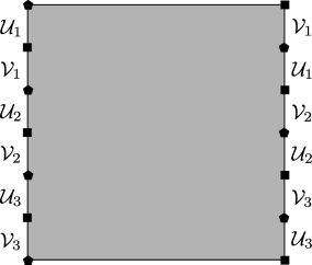
Figure 5. The space $Q(\mathcal{S})$ for $\mathcal{S}=\Sigma_{3,1}$. The black pentagons represent the point $\mathcal{P}_{even}$, whereas the black squares represent $\mathcal{P}_{odd}$.

Our next aim is to define a structure of $CW$-complex on the space $C_{m}(\mathcal{S})^{\infty}$: the only $0$-cell will be the point $\infty$, whereas the other cells will be introduced in the following definition.

Definition 3.4.

A tuple $\mathfrak{h}$ is a choice of the following set of data:

• a natural number $0\leq l\leq m$;

• a vector $\underline{x}=(x_{1},\dots,x_{l})$ of integers $\geq 1$;

• vectors $\underline{u}=(u_{1},\dots,u_{g})$ and $\underline{v}=(v_{1},\dots,v_{g})$ of integers $\geq 0$,

satisfying the following equality

$$m=\sum_{i=1}^{l}x_{i}+\sum_{i=1}^{g}(u_{i}+v_{i}).$$

In symbols we write $\mathfrak{h}=(l,\underline{x},\underline{u},\underline{v})$. We omit from the notation $\underline{x}$ if it vanishes: this happens precisely when $l=0$. The dimension of $\mathfrak{h}$ is defined as $m+l$.

For a tuple $\mathfrak{h}$ let $e^{\mathfrak{h}}$ be the subspace of $C_{m}(\mathcal{S})$ of configurations of $m$ points in $\mathring{\mathcal{S}}$ such that the following conditions hold (see picture 6):

• for all $1\leq i\leq g$, exactly $u_{i}$ points lie on $\mathcal{U}_{i}$ and exactly $v_{i}$ points lie on $\mathcal{V}_{i}$;

• there are exactly $l$ vertical lines in the open square $]0,1[^{2}\subset\mathring{\mathcal{S}}$ of the form $\left\{s_{i}\right\}\times]0,1[$ for some $0<s_{1}<\dots<s_{l}<1$, containing at least one point of the configuration. From left to right, these lines contain exactly $x_{1},\dots,x_{l}$ points respectively.

Figure 6. A configuration in the subspace $e^{\mathfrak{h}}\subset C_{14}(\mathcal{S})$, for the tuple $\mathfrak{h}=(3,(3,1,2),(1,2,0),(0,3,2))$. Points lying on the $\mathcal{U}_{i}$’s and the $\mathcal{V}_{i}$’s are depicted twice.

The space $e^{\mathfrak{h}}$ is homeomorphic to the interior of the following multisimplex:

$$\Delta^{\mathfrak{h}}\colon=\Delta^{l}\times\prod_{i=1}^{l}\Delta^{x_{i}}\times\prod_{i=1}^{g}\left(\Delta^{u_{i}}\times\Delta^{v_{i}}\right),$$

where the simplex $\Delta^{r}$ is the subspace of $[0,1]^{r}$ of sequences $0\leq\tau_{1}\leq\dots\leq\tau_{r}\leq 1$ (the numbers $\tau_{1},\dots,\tau_{r}$ are the local coordinates of the simplex). The homeomorphism is given as follows:

• the local coordinates of the $\Delta^{l}$-factor correspond to the positions $s_{1},\dots,s_{l}$ of the vertical lines in $(0,1)^{2}$ containing points of the configuration;

• the local coordinates of the $\Delta^{x_{i}}$-factor correspond to the positions of the $x_{i}$ points lying on the vertical line $\left\{s_{i}\right\}\times(0,1)$;

• the local coordinates of the $\Delta^{u_{i}}$-factor correspond to the positions of the $u_{i}$ points lying on $\mathcal{U}_{i}$, which is canonically identified with $(0,1)$; similarly for the $\Delta^{v_{i}}$-factor, with $v_{i}$ and $\mathcal{V}_{i}$ replacing $u_{i}$ and $\mathcal{U}_{i}$.

Note that the dimension of $\Delta^{\mathfrak{h}}$ agrees with the dimension of $\mathfrak{h}$ from Definition 3.4. The embedding $\mathring{\Delta}^{\mathfrak{h}}\cong e^{\mathfrak{h}}\hookrightarrow C_{m}(\mathcal{S})^{\infty}$ extends to a continuous map $\Phi^{\mathfrak{h}}\colon\Delta^{\mathfrak{h}}\to C_{m}(\mathcal{S})^{\infty}$, so that the image of $\partial\Delta^{\mathfrak{h}}$ is contained in the union of all subspaces $e^{\mathfrak{h}^{\prime}}$ for tuples $\mathfrak{h}^{\prime}$ of lower dimension than $\mathfrak{h}$, together with the $0$-cell $\infty$.

The construction of the map $\Phi^{\mathfrak{h}}$ is as follows:

1. we identify the one-point compactification $(\mathring{\mathcal{S}})^{\infty}$ of $\mathring{\mathcal{S}}=\mathcal{T}(\mathcal{S})$ as the quotient of $Q(\mathcal{S})$ collapsing the boundary to a point $\infty$;

2. we consider the $m$-fold symmetric product $S\!P^{m}\left((\mathring{\mathcal{S}})^{\infty}\right)$ (see Definition 2.5): it contains as an open subspace $C_{m}(\mathcal{S})$, so we can identify $C_{m}(\mathcal{S})^{\infty}$ as the quotient of $S\!P^{m}\left((\mathring{\mathcal{S}})^{\infty}\right)$ collapsing the subspace $S\!P^{m}\left((\mathring{\mathcal{S}})^{\infty}\right)\setminus C_{m}(\mathcal{S})$ to $\infty$;

3. the homeomorphism $\mathring{\Delta}^{\mathfrak{h}}\to e^{\mathfrak{h}}\subset C_{m}(\mathcal{S})$ extends now to a map $\Delta^{\mathfrak{h}}\to S\!P^{m}\left([0,1]^{2}\right)$, that we can then further project to $S\!P^{m}(Q(\mathcal{S}))$, then to $S\!P^{m}\left((\mathring{\mathcal{S}})^{\infty}\right)$ and then to $C_{m}(\mathcal{S})^{\infty}$: the composition is the map $\Phi^{\mathfrak{h}}$.

In the last step we used the open inclusion $C_{m}(\mathcal{S})\subset S\!P^{m}\left(\mathring{\mathcal{S}}\right)\subset S\!P^{m}\left((\mathring{\mathcal{S}})^{\infty}\right)$, which induces a map $S\!P^{m}\left((\mathring{\mathcal{S}})^{\infty}\right)\to C_{m}(\mathcal{S})^{\infty}$ by quotienting to $\infty$ the closed subspace $S\!P^{m}\left((\mathring{\mathcal{S}})^{\infty}\right)\setminus C_{m}(\mathcal{S})^{\infty}$.

We conclude that the collection of the $e^{\mathfrak{h}}$’s, together with the $0$-cell $\infty$, gives a cell decomposition of $C_{m}(\mathcal{S})^{\infty}$, with characteristic maps of cells $\Phi^{\mathfrak{h}}$.

We compute the reduced cellular chain complex of $C_{m}(\mathcal{S})^{\infty}$ with coefficients in $\mathbb{Z}_{2}$. It is a chain complex in $\mathbb{Z}_{2}$-vector spaces with basis given by tuples $\mathfrak{h}$, which correspond to the cells $e^{\mathfrak{h}}$.

Lemma 3.5.

Let $\mathfrak{h}=(l,\underline{x},\underline{u},\underline{v})$ and $\mathfrak{h}^{\prime}=(l-1,\underline{x}^{\prime},\underline{u}^{\prime},\underline{v}^{\prime})$ be tuples in consecutive dimensions $m+l$ and $m+l-1$. Denote by $[\mathfrak{h}\colon\mathfrak{h}^{\prime}]\in\mathbb{Z}_{2}$ the coefficient of $\mathfrak{h}^{\prime}$ in $\partial\mathfrak{h}$ in the reduced chain complex $\tilde{\mathcal{C}}_{*}(C_{m}(\mathcal{S})^{\infty})$. Then $[\mathfrak{h}:\mathfrak{h}^{\prime}]=0$ unless one, and exactly one, of the following situations occurs:

• $l\geq 2$ and $\mathfrak{h}^{\prime}$ is obtained from $\mathfrak{h}$ by decreasing $l$ by 1, setting $x^{\prime}_{i}=x_{i}+x_{i+1}$ for one value $1\leq i\leq l-1$, and shifting the values $x^{\prime}_{j}=x_{j+1}$ for $i+1\leq j\leq l-1$. In this case we say that $\mathfrak{h}^{\prime}$ is an inner boundary of $\mathfrak{h}$, and we have

  $$[\partial\mathfrak{h}\colon\mathfrak{h}^{\prime}]=\binom{x_{i}+x_{i+1}}{x_{i}}\in\mathbb{Z}_{2},$$

  where $\binom{x_{i}+x_{i+1}}{x_{i}}$ denotes the binomial coefficient.

• $l\geq 1$ and $\mathfrak{h}^{\prime}$ is obtained from $\mathfrak{h}$ by decreasing $l$ by 1, choosing a splitting of $x_{1}$ in integers $\tilde{u}_{i},\tilde{v}_{i}\geq 0$

  $$x_{1}=\sum_{i=1}^{g}\left(\tilde{u}_{i}+\tilde{v}_{i}\right),$$

  setting $u^{\prime}_{i}=u_{i}+\tilde{u}_{i}$ and $v^{\prime}_{i}=v_{i}+\tilde{v}_{i}$ for all $1\leq i\leq g$ and shifting the values $x^{\prime}_{j}=x_{j+1}$ for $1\leq j\leq l-1$. In this case we say that $\mathfrak{h}^{\prime}$ is a left, outer boundary of $\mathfrak{h}$, and we have

  $$[\partial\mathfrak{h}\colon\mathfrak{h}^{\prime}]=\prod_{i=1}^{g}\binom{u_{i}+\tilde{u}_{i}}{u_{i}}\binom{v_{i}+\tilde{v}_{i}}{v_{i}}\in\mathbb{Z}_{2}.$$

• $l\geq 1$ and $\mathfrak{h}^{\prime}$ is obtained from $\mathfrak{h}$ by decreasing $l$ by 1, choosing a splitting of $x_{l}$ in integers $\tilde{u}_{i},\tilde{v}_{i}\geq 0$

  $$x_{l}=\sum_{i=1}^{g}\left(\tilde{u}_{i}+\tilde{v}_{i}\right),$$

  setting $u^{\prime}_{i}=u_{i}+\tilde{u}_{i}$ and $v^{\prime}_{i}=v_{i}+\tilde{v}_{i}$ for all $1\leq i\leq g$ and keeping $x^{\prime}_{i}=x_{i}$ for all $1\leq i\leq l-1$. In this case we say that $\mathfrak{h}^{\prime}$ is a right, outer boundary of $\mathfrak{h}$, and we have

  $$[\partial\mathfrak{h}\colon\mathfrak{h}^{\prime}]=\prod_{i=1}^{g}\binom{u_{i}+\tilde{u}_{i}}{u_{i}}\binom{v_{i}+\tilde{v}_{i}}{v_{i}}\in\mathbb{Z}_{2}.$$

It may indeed happen that $\mathfrak{h}^{\prime}$ is both a left and a right outer boundary of $\mathfrak{h}$, namely when all numbers $(x_{i})_{1\leq i\leq l}$ are equal; then the two contributions cancel each other, so that $[\mathfrak{h}\colon\mathfrak{h}^{\prime}]=0$ as stated.

Proof.

For $1\leq i\leq l$ denote by $\partial^{hor}_{i}\Delta^{\mathfrak{h}}$ the face

$$\partial_{i}\Delta^{l}\times\prod_{i=1}^{l}\Delta^{x_{i}}\times\prod_{i=1}^{g}\left(\Delta^{u_{i}}\times\Delta^{v_{i}}\right)\subset\Delta^{\mathfrak{h}}.$$

This is also referred as the $i$-th horizontal face. All other faces of codimension 1 of the multisimplex $\Delta^{\mathfrak{h}}$ are called vertical.

We note that $\Phi^{\mathfrak{h}}$ restricts to a cellular map $\partial_{i}^{hor}\Delta^{\mathfrak{h}}\to C_{m}(\mathcal{S})^{\infty}$ on every horizontal face, where $\partial_{i}^{hor}\Delta^{\mathfrak{h}}$ is given the cell structure coming from the multisimplicial structure: every subface of $\partial_{i}^{hor}\Delta^{\mathfrak{h}}$ of dimension $k\leq m+l-1$ is mapped to the $k$-skeleton of $C_{m}(\mathcal{S})^{\infty}$. Therefore the map $\Phi^{\mathfrak{h}}\colon\partial_{i}^{hor}\Delta^{\mathfrak{h}}\to C_{m}(\mathcal{S})^{\infty}$ has a well-defined local index over the cell $e^{\mathfrak{h}^{\prime}}$, that we call $[\partial^{hor}_{i}\mathfrak{h}\colon\mathfrak{h}^{\prime}]\in\mathbb{Z}_{2}$.

The same holds for vertical faces, where the restriction of $\Phi^{\mathfrak{h}}$ is the constant map to $\infty$: in this case the local index over $e^{\mathfrak{h}^{\prime}}$ is zero. The index $[\mathfrak{h}\colon\mathfrak{h}^{\prime}]$ of the map $\Phi^{\mathfrak{h}}\colon\partial\Delta^{\mathfrak{h}}\to C_{m}(\mathcal{S})^{\infty}$ on $e^{\mathfrak{h}^{\prime}}$ splits as a sum of local indices:

$$[\mathfrak{h}\colon\mathfrak{h}^{\prime}]=\sum_{i=0}^{l}[\partial_{i}^{hor}\mathfrak{h}\colon\mathfrak{h}^{\prime}]\in\mathbb{Z}_{2}.$$

For $0\leq i\leq l$ the restriction $\Phi^{\mathfrak{h}}\colon\partial^{hor}_{i}\Delta^{\mathfrak{h}}\to C_{m}(\mathcal{S})^{\infty}$ hits homeomorphically the open cell $e^{\mathfrak{h}^{\prime}}$ exactly as many times as specified in the statement of the lemma for the cases $1\leq i\leq l-1$, $i=0$ and $i=l$ respectively.

The only possibility in which the same cell $e^{\mathfrak{h}^{\prime}}$ is hit by different faces $\partial_{i}^{hor}\Delta^{\mathfrak{h}}$ and $\partial_{j}^{hor}\Delta^{\mathfrak{h}}$ is the one described in the remark preceding this proof: in this case there are two equal contributions $[\partial_{i}^{hor}\mathfrak{h}\colon\mathfrak{h}^{\prime}]$ and $[\partial_{j}^{hor}\mathfrak{h}\colon\mathfrak{h}^{\prime}]$ that cancel each other. ∎

We can filter the reduced chain complex $\tilde{\mathcal{C}}_{*}(C_{m}(\mathcal{S})^{\infty})$ by giving filtration norm $\sum_{i=1}^{l}x_{i}$ to the tuple $\mathfrak{h}=(l,\underline{x},\underline{u},\underline{v})$, with $\underline{x}=(x_{1},\dots,x_{l})$. For example the tuple in Figure 6 has norm 6.

By Lemma 3.5 the norm is weakly decreasing along differentials. Denote by $F_{p}\subset\tilde{\mathcal{C}}_{*}(C_{m}(\mathcal{S})^{\infty})$ the subcomplex generated by tuples of norm $\leq p$, and let $F_{p}/F_{p-1}$ be the $p$-th filtration stratum. Then $F_{p}/F_{p-1}$ is isomorphic, as a chain complex, to a direct sum of copies of $\tilde{\mathcal{C}}_{*}(C_{p}(\Sigma_{0,1})^{\infty})$: there is one copy for each partition

$$(m-p)=\sum_{i=1}^{g}(u_{i}+v_{i})$$

with $u_{i},v_{i}\geq 0$. The isomorphism does not preserve the degrees but shifts them by $p$.

Indeed in $F_{p}/F_{p-1}$ all outer differentials vanish (see Lemma 3.5): in particular the numbers $u_{i},v_{i}$ do not change along the differentials of $F_{p}/F_{p-1}$. Therefore $F_{p}/F_{p-1}$ splits as a direct sum of chain complexes indexed by all partitions $(m-p)=\sum_{i=1}^{g}(u_{i}+v_{i})$ as above. It is then immediate to identify the inner faces with the ones one would have in the case $g=0$, i.e. for the surface $\Sigma_{0,1}$, after shifting degrees by $p$.

We note that $\tilde{\mathcal{C}}_{*}(C_{p}(\Sigma_{0,1})^{\infty})$ is exactly the chain complex described by Fuchs in [9]: we recall Fuchs’ computation of the cohomology of configuration spaces of the disc, and abbreviate $\mathcal{D}$ for $\mathring{\Sigma}_{0,1}$ as in Section 2.

Definition 3.6.

Consider a partition of $p$ into powers of 2

$$p=\sum_{j\geq 0}\alpha_{j}2^{j},$$

and let $\underline{\alpha}=(\alpha_{j})_{j\geq 0}$ be the sequence of multiplicities. We understand that only finitely many $\alpha_{j}$’s are strictly positive.

The associated symmetric chain in $\tilde{\mathcal{C}}_{*}(C_{p}(\mathcal{D})^{\infty})$, denoted by $\kappa(\underline{\alpha})$, is the sum of all tuples $\mathfrak{h}=\left(l,(x_{i})_{i\leq l}\right)$ such that

• $l=\sum_{j\geq 0}\alpha_{j}$;

• every $x_{i}$ is a power of 2;

• for all $j\geq 0$ there are exactly $\alpha_{j}$ indices $i$ such that $x_{i}=2^{j}$.

A symmetric chain $\kappa(\underline{\alpha})$ is a cycle in the chain complex $\tilde{\mathcal{C}}_{*}(C_{p}(\mathcal{D})^{\infty})$ (see [9]). We denote by $[\kappa(\underline{\alpha})]\in\tilde{H}_{p+l}(C_{p}(\mathcal{D})^{\infty})$ the associated homology class.

In [9] Fuchs shows that a graded basis for $\tilde{H}_{*}(C_{p}(\mathcal{D})^{\infty})$ is given by the collection of all classes $[\kappa(\underline{\alpha})]$ associated to sequences $\underline{\alpha}=(\alpha_{j})_{j\geq 0}$ which satisfy the equality $p=\sum_{j\geq 0}\alpha_{j}2^{j}$.

By Poincaré-Lefschetz duality this corresponds to a basis for $H^{*}(C_{p}(\mathcal{D}))$. The dual basis of $H_{*}(C_{p}(\mathcal{D}))$ happens to be the basis of monomials

$$Q^{\underline{\alpha}}\varepsilon\colon=\prod_{j\geq 0}(Q^{i}\varepsilon)^{\alpha_{j}}\in H_{*}(C_{p}(\mathcal{D})).$$

This basis consists of all monomials of weight $p$, using the isomorphism (5) in its full meaning (i.e. as an isomorphism of rings, where $Q$ denotes the first Dyer-Lashof operation).

We will not need this finer result in this article, so in the following the expression $Q^{\underline{\alpha}}$ will only denote the (unique) homology class in $H_{p-l}(C_{p}(\mathcal{D}))$ such that the following holds: for all $\underline{\alpha}^{\prime}=(\alpha^{\prime}_{j})_{j\geq 0}$ with $\sum_{j\geq 0}\alpha^{\prime}_{j}=p$, the algebraic intersection between $Q^{\underline{\alpha}}\varepsilon\in H_{p-l}(C_{p}(\mathcal{D}))$ and $[\kappa(\underline{\alpha}^{\prime})]\in\tilde{H}_{p+l}(C_{p}(\mathcal{D})^{\infty})$ is $1\in\mathbb{Z}_{2}$ if and only $\underline{\alpha}=\underline{\alpha}^{\prime}$.

We now go back to the filtered chain complex $\tilde{\mathcal{C}}_{*}(C_{m}(\mathcal{S})^{\infty})$. The $E^{1}$-page of the associated Leray spectral sequence contains on the $p$-th column the homology of $F_{p}/F_{p-1}$; as we have seen the homology of this filtration stratum is the direct sum of several copies of the homology of $\tilde{\mathcal{C}}_{*}(C_{p}(\mathcal{D}))$, one copy for each partition $(m-p)=\sum_{i=1}^{g}(u_{i}+v_{i})$ with $u_{i},v_{i}\geq 0$.

Definition 3.7.

Consider a partition

$$m=p+(m-p)=\left(\sum_{j=0}^{\infty}\alpha_{j}2^{j}\right)+\left(\sum_{i=1}^{g}(u_{i}+v_{i})\right)$$

and let $\underline{u}=(u_{1},\dots,u_{g})$, $\underline{v}=(v_{1},\dots,v_{g})$, $\underline{\alpha}=(\alpha_{j})_{j\geq 0}$; denote also $l=\sum_{j=0}^{\infty}\alpha_{j}$.

We define a chain $\kappa(p,\underline{\alpha},\underline{u},\underline{v})$ in $\tilde{\mathcal{C}}_{m+l}(C_{m}(\mathcal{S}))$: it is the sum of all tuples $\mathfrak{h}$ of the form $\left(l,\underline{x},\underline{u},\underline{v}\right)$, for varying $\underline{x}$, which satisfy the three properties listed in Definition 3.6.

We call such a chain a generalised symmetric chain; we will see in the following that it is a cycle, and we will denote by $[\kappa(p,\underline{\alpha},\underline{u},\underline{v})]$ the associated homology class in $\tilde{H}_{m+l}(C_{m}(\mathcal{S})^{\infty})$.

If any of $\underline{\alpha}$, $\underline{u}$ and $\underline{v}$ vanishes, we omit it from the notation.

A generalised symmetric chain $\kappa(p,\underline{\alpha},\underline{u},\underline{v})$ is not only a cycle when projected to its filtration quotient $F_{p}/F_{p-1}$, as the $E^{1}$-page of the spectral sequence tells us, but also in the chain complex $\tilde{\mathcal{C}}_{*}(C_{m}(\mathcal{S})^{\infty})$ itself.

To prove this fact, first note that an inner boundary of a tuple $\mathfrak{h}$ preserves the norm; hence the fact that $\kappa(p,\underline{\alpha},\underline{u},\underline{v})$ is a cycle in $F_{p}/F_{p-1}$ guarantees the fact that all inner boundaries of $\kappa(p,\underline{\alpha},\underline{u},\underline{v})$ cancel each other in $\tilde{\mathcal{C}}_{*}(C_{m}(\mathcal{S})^{\infty})$, that is,

$$\partial\kappa(p,\underline{\alpha},\underline{u},\underline{v})\in\tilde{\mathcal{C}}_{*}(C_{m}(\mathcal{S})^{\infty})$$

is equal to the sum of all outer boundaries of the tuples involved.

Note now that outer boundaries of a generalised symmetric chain also cancel out: the left outer boundary of a tuple $\mathfrak{h}=(l,\underline{x},\underline{u},\underline{v})$ in the generalised symmetric chain cancels against the right outer boundary of the tuple $\mathfrak{h}^{\prime}=(l,\underline{x}^{\prime},\underline{u},\underline{v})$, with $x^{\prime}_{l}=x_{1}$ and $x^{\prime}_{i}=x_{i+1}$ for $1\leq i\leq l-1$. If all $x_{i}$ happen to be equal, then $\mathfrak{h}=\mathfrak{h}^{\prime}$ and we are in the situation described before the proof of Lemma 3.5.

The spectral sequence considered above collapses on its first page and we have the following lemma:

Lemma 3.8.

The homology $H_{*}(C_{m}(\mathcal{S})^{\infty})$ has a graded basis given by the classes $[\kappa(p,\underline{\alpha},\underline{u},\underline{v})]$ associated to generalised symmetric chains of weight $m$.

Definition 3.9.

We can see the $\mathcal{U}_{i}$’s and $\mathcal{V}_{i}$’s as properly embedded $1$-manifolds in $\mathring{\mathcal{S}}$; by Poincaré-Lefschetz duality they represent classes in $\tilde{H}_{1}\left((\mathring{\mathcal{S}})^{\infty}\right)\simeq H^{1}(\mathcal{S})$, and in particular they form a basis of the latter cohomology group. We call $\mathfrak{u}_{i},\mathfrak{v}_{i}\in H_{1}\left(\mathring{\mathcal{S}}\right)$ the dual basis.

We establish a bijection between monomials in the tensor product of Theorem 3.2 and the basis of $H^{*}(C_{m}(\mathcal{S}))\simeq H_{*}(C_{m}(\mathcal{S})^{\infty})$ in Lemma 3.8: the class

$$[\kappa(p,\underline{\alpha},\underline{u},\underline{v})]\in H_{m+\sum\alpha_{j}}(C_{m}(\mathcal{S})^{\infty})\simeq H^{m-\sum\alpha_{j}}(C_{m}(\mathcal{S}))$$

is associated with the monomial

$$Q^{\underline{\alpha}}\varepsilon\cdot\mathfrak{u}^{\underline{u}}\cdot\mathfrak{v}^{\underline{v}}\colon=\prod_{j=1}^{\infty}(Q^{j}\varepsilon)^{\alpha_{j}}\otimes\prod_{i=1}^{g}(\mathfrak{u}_{i}^{u_{i}}\mathfrak{v}_{i}^{v_{i}}),$$

where $\underline{\alpha}=(\alpha_{j})_{j\geq 0}$, $\underline{u}=(u_{1},\dots,u_{g})$ and $\underline{v}=(v_{1},\dots,v_{g})$.

This shows an isomorphism of bigraded $\mathbb{Z}_{2}$-vector spaces

(6) $$\bigoplus_{m\geq 0}H^{*}(C_{m}(\mathcal{S}))\simeq\mathbb{Z}_{2}\left[Q^{j}\varepsilon\,|\,j\geq 0\right]\otimes\operatorname{Sym}_{\bullet}(\mathcal{H}),$$

from which we conclude that there exists an isomorphism as in Theorem 3.2 at least as bigraded $\mathbb{Z}_{2}$-vector spaces: the two bigraded vector spaces have the same dimension in all bigradings.

4. Action of $\Gamma_{g,1}$

We now turn back to homology of $C_{m}(\mathcal{S})$. In the first subsection we describe geometrically some homology classes, in order to give some intuition for the following subsections. In the second subsection we prove Theorem 3.2 in bigradings $(*,m)$ with $*=m$. In the third subsection we extend the proof to all other bigradings.

4.1. Geometric examples of homology classes

In this subsection we consider the case $g=2$, hence $\mathcal{S}$ denotes the surface $\Sigma_{2,1}$. We construct some homology classes in $H_{2}(C_{2}(\mathcal{S}))$: our aim is to get a first understanding of why this homology group is isomorphic to $\operatorname{Sym}_{2}(\mathcal{H})=\mathcal{H}^{\otimes 2}/\mathfrak{S}_{2}$; the notation $\mathcal{H}=H_{1}(\mathcal{S})$ was introduced in Definition 3.1.

In the following $c$ and $d$ will always denote two simple closed curves on $\mathcal{S}$, with corresponding homology classes $[c],[d]\in\mathcal{H}$.

Example 1.

Suppose that $c$ and $d$ are as in Figure 7: $c$ and $d$ are disjoint and non-separating. We can consider inside $C_{2}(\mathcal{S})$ the torus $c\times d$ of configurations in which one of the two points runs along $c$, while the other runs along $d$. We associate to the fundamental class $\tau_{1}\in H_{2}(C_{2}(\mathcal{S}))$ of this torus the tensor product $[c]\otimes[d]\in\mathcal{H}^{\otimes 2}$.

Since our configurations are unordered and since we work with coefficients in $\mathbb{Z}_{2}$, the same class $\tau_{1}$ can be obtained as a tensor product $[d]\otimes[c]$, i.e. exchanging the order of the two curves: we can neglect the sign $-1$ that this operation would generate. We represent $\tau_{1}$ as $[c]\cdot[d]\in\operatorname{Sym}_{2}(\mathcal{H})$.

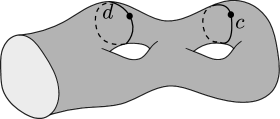
Figure 7.

Example 2.

Suppose that $c$ and $d$ are as in Figure 8: $c$ and $d$ are disjoint, and $c$ bounds a subsurface $\check{\mathcal{S}}$ of $\mathcal{S}$ (the shaded region), such that $d$ is not contained in $\check{\mathcal{S}}$.

Then the homology class $\tau_{2}=[c]\cdot[d]$ vanishes, because the torus $c\times d$ is the boundary in $C_{2}(\mathcal{S})$ of the 3-manifold $\check{\mathcal{S}}\times d$ containing all configurations in which one point lies on $\check{\mathcal{S}}$ and the other on $d$. This is consistent with the representation $\tau_{2}=[c]\cdot[d]$, because $[c]=0\in\mathcal{H}$.

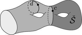
Figure 8.

Example 3.

Suppose that $c$ and $d$ are as in Figure 9: $c$ and $d$ are non-separating and intersect transversely in one point $P\in\mathcal{S}$. In this case the torus $c\times d$ is a subspace of $S\!P^{2}(\mathcal{S})$, but $c\times d$ is not contained in $C_{2}(\mathcal{S})$ as in Example 1.

To solve this problem, we consider a small open neighborhood $P\in\mathcal{U}\subset\mathcal{S}$, and we remove from the torus $c\times d$ all configurations in which both points lie in $\mathcal{U}$: these removed configurations form an open disc inside the torus $c\times d$.

We obtain an embedding $\Sigma_{1,1}\hookrightarrow C_{2}(\mathcal{S})$; the boundary $\partial\Sigma_{1,1}$, seen as a curve in $C_{2}(\mathcal{S})$, is homotopic to a curve $\gamma$ in which one point spins $360^{\circ}$ around the other. We note that the curve $\gamma\subset C_{2}(\mathcal{S})$ is homotopic to a double covering of a curve $\gamma^{\prime}\subset C_{2}(\mathcal{S})$, in which the two points exchange their positions after spinning $180^{\circ}$ around each other. All curves $\partial\Sigma_{1,1}$, $\gamma$, $\gamma^{\prime}$ and the homotopies relating them are supported on the closure of $C_{2}(\mathcal{U})$ in $C_{2}(\mathcal{S})$.

We can therefore find a map from a Möbius band $\mathcal{M}$ to the closure of $C_{2}(\mathcal{U})$ in $C_{2}(\mathcal{S})$, such that the images of the curves $\partial\mathcal{M}$ and $\partial\Sigma_{1,1}$ in $C_{2}(\mathcal{S})$ coincide. The union $\Sigma_{1,1}\cup_{\partial}\mathcal{M}$ along the boundary is then a closed non-orientable surface of genus $3$, i.e. the connected sum of a torus and a projective plane.

The surface $\Sigma_{1,1}\cup_{\partial}\mathcal{M}$ is equipped with a map to $C_{2}(\mathcal{S})$, hence its fundamental class with coefficients in $\mathbb{Z}_{2}$ yields a homology class $\tau_{3}\in H_{2}(C_{2}(\mathcal{S}))$; thus we have managed to adapt the construction from Example 1 to the case of two intersecting curves. We represent $\tau_{3}$ as $[c]\cdot[d]\in\operatorname{Sym}_{2}(\mathcal{H})$.

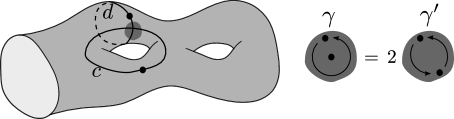
Figure 9.

Example 4.

Suppose that $c$ and $d$ are as in Figure 10: $c$ and $d$ are disjoint, and $c$ bounds a subsurface $\check{\mathcal{S}}$ of $\mathcal{S}$ (the shaded region), such that $d$ is contained in $\check{\mathcal{S}}$.

The torus $c\times d$ is contained in $C_{2}(\mathcal{S})$, but it is not obvious, at first glance, why its corresponding homology class $\tau_{4}\in H_{2}(C_{2}(\mathcal{S}))$ should vanish: the argument used in Example 2 does not work immediately, because the 3-manifold $\check{\mathcal{S}}\times d$ is only contained in $S\!P^{2}(\mathcal{S})$ and not in $C_{2}(\mathcal{S})$.

We try to modify this 3-manifold in the same spirit of Example 3. Let $\mathcal{U}\tilde{\times}d\subset\check{\mathcal{S}}\times d$ be an open tubular neighborhood of $d\times d$: note that this tubular neighborhood is a trivial bundle over $d$ with fiber an open disc $\mathcal{U}$. The notation $\tilde{\times}$ means that abstractly we are dealing with a product $\mathcal{U}\times d$, but not geometrically: fibers over different points of $d$ are naturally identified with different discs in $\check{\mathcal{S}}$.

We consider the 3-manifold $\check{\mathcal{S}}\times d\setminus\mathcal{U}\tilde{\times}d$: its boundary is the disjoint union of the torus $c\times d$ and the torus $\partial\left(\mathcal{U}\tilde{\times}d\right)$. The latter torus contains configurations of two points in $\mathcal{S}$, one of which spins around $d$, whereas the other is a satellite of the first and spins around it $360^{\circ}$.

We regard $\partial\mathcal{U}\tilde{\times}d$ as a trivial bundle $\gamma\tilde{\times}d$ over $d$, with fiber the curve $\gamma$ considered in Example 3. After a homotopy the latter torus becomes a double covering of a torus $\gamma^{\prime}\tilde{\times}d$: this is a trivial bundle over $d$ with fiber the curve $\gamma^{\prime}$; we can see $\gamma^{\prime}\tilde{\times}d\subset C_{2}(\mathcal{S})$ as a torus of configurations in which the two points exchange their positions spinning $180^{\circ}$ around each other, while their barycenter spins around $d$.

We can fill the second boundary of the $3$-manifold $\check{\mathcal{S}}\times d\setminus\mathcal{U}\tilde{\times}d$ with the product $\mathcal{M}\times d$: the output is a non-orientable $3$-manifold with boundary $c\times d$, witnessing that $\tau_{4}=0$.

This is consistent with the representation $\tau_{4}=[c]\cdot[d]$, because $[c]=0\in\mathcal{H}$.

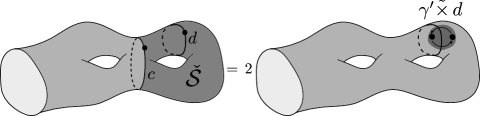
Figure 10.

Example 5.

Suppose that $c$ and $d$ are as in Figure 11: $c$ bounds a subsurface $\check{\mathcal{S}}$, and $d$ is cut by $c$ into two arcs, one of which, denoted by $e$, lies in $\check{\mathcal{S}}$.

In this example the complications from Examples 3 and 4 arise at the same time.

To define the class $\tau_{5}\in H_{2}(C_{2}(\mathcal{S}))$, we start with the torus $c\times d$ and we perform two surgeries with two different Möbius bands to solve the two intersections of $c$ and $d$: the homology class that we obtain is represented by a non-orientable surface of genus 4, i.e. the connected sum of a torus and 2 projective planes.

To show that $\tau_{5}$ vanishes, we start with the 3-manifold with boundary $\check{\mathcal{S}}\times d\subset S\!P^{2}(\mathcal{S})$ and we perform a surgery. We identify with $e$ the arc

$$\check{\mathcal{S}}\times d\cap\left(S\!P^{2}(\mathcal{S})\setminus C_{2}(\mathcal{S})\right);$$

this is a properly embedded arc in the 3-manifold with boundary $\check{\mathcal{S}}\times d$, and a tubular neighborhood of it, after a suitable homotopy, can be identified with a trivial $\mathcal{U}$-bundle $\mathcal{U}\tilde{\times}e$. We remove this solid cylinder from the 3-manifold and glue a trivial $\mathcal{M}$-bundle $\mathcal{M}\tilde{\times}e$, by applying an argument similar as the one in Examples 3 and 4.

We obtain a 3-manifold with boundary endowed with a map to $C_{2}(\mathcal{S})$; the boundary of this 3-manifold is precisely the surface used to represent $\tau_{5}$: therefore $\tau_{5}=0\in H_{2}(C_{2}(\mathcal{S}))$, and this is consistent with the representation $\tau_{5}=[c]\cdot[d]$, because $[c]=0\in\mathcal{H}$.

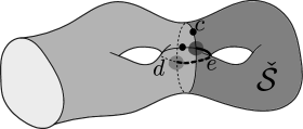
Figure 11.

If we consider more than 2 points, the examples become more and more complicated, and proving the theorem with this geometric approach seems rather difficult.

4.2. Bigradings of the form $(m,m)$

In this subsection we construct a $\Gamma_{g,1}$- equivariant isomorphism

$$\psi_{m}\colon\operatorname{Sym}_{m}(\mathcal{H}))\to H_{m}(C_{m}(\mathcal{S})).$$

We already know that these $\mathbb{Z}_{2}$-vector spaces have the same dimension: indeed $\operatorname{Sym}_{m}(\mathcal{H})$ is precisely the summand in bigrading $(m,m)$ in equation (6), using that a monomial whose weight is equal and not bigger than its degree cannot contain factors of the form $Q^{i}\varepsilon$.

The construction of $\psi_{m}$ is rather long and technical and involves a few definitions.

Definition 4.1.

Recall Definition 3.3. We denote by $\mathcal{D}\subset\mathcal{T}(\mathcal{S})\cong\mathring{\mathcal{S}}$ the open square $]1/4;3/4[\times]1/2,1[$. Note that $\mathcal{D}$ is an open disc in $\mathring{\mathcal{S}}$ near $\partial\mathcal{S}$ and it is disjoint from all $\overline{\mathcal{U}}_{i}$’s and $\overline{\mathcal{V}}_{i}$’s. The interior of the surface $\mathcal{S}^{\prime}$ is then identified with $\mathcal{T}(\mathcal{S})\setminus[1/4,3/4]\times[1/2,1[$.

Definition 4.2.

Let $\mathfrak{C}^{m}$ be the the (discrete) set of isotopy classes of $m$-tuples of simple closed curves $c_{1},\dots,c_{m}\subset\mathring{\mathcal{S}}$ such that any two curves $c_{i},c_{j}$ intersect each other only inside $\mathcal{D}$.

Curves are seen as maps $\mathbb{S}^{1}\to\mathring{\mathcal{S}}$, and the intersection of two curves is the intersection of their images. Here and in the following $\mathbb{S}^{1}$ is the unit circle in $\mathbb{C}$.

Two $m$-tuples of curves are isotopic if there is an ambient isotopy of $\mathcal{S}$ relative to $\partial\mathcal{S}\cup\mathcal{D}$ transforming one $m$-tuple into the other. In particular $\mathfrak{C}^{m}$ is more than countable.

An element of $\mathfrak{C}^{m}$ is called multicurve; by abuse of notation the $m$-tuple $(c_{1},\dots,c_{m})$ will often represent its class in $\mathfrak{C}^{m}$, i.e. the corresponding multicurve. See picture 12

We denote by $\mathbb{Z}_{2}\left<\mathfrak{C}^{m}\right>$ the free $\mathbb{Z}_{2}$-vector space with basis $\mathfrak{C}^{m}$. There is a canonical surjective map $\mathfrak{p}_{m}\colon\mathbb{Z}_{2}\left<\mathfrak{C}^{m}\right>\to\operatorname{Sym}_{m}(\mathcal{H})$ given by

$$\mathfrak{p}_{m}(c_{1},\dots,c_{m})=[c_{1}]\cdot\ldots\cdot[c_{m}],$$

where $[c_{i}]\in\mathcal{H}$ is the fundamental class of the curve $c_{i}$.

The group $\Gamma_{g,1}$ acts both on $\mathbb{Z}_{2}\left<\mathfrak{C}^{m}\right>$, by acting on its basis $\mathfrak{C}^{m}$, and on $\operatorname{Sym}_{m}(\mathcal{H})$, symplectically. The map $\mathfrak{p}_{m}$ is $\Gamma_{g,1}$-equivariant.

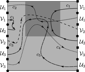
Figure 12. A multicurve in $\mathfrak{C}^{5}$.

Definition 4.3.

Recall Definition 2.5. The space $C_{m}^{\mathcal{D}}(\mathcal{S})$ is the subspace of $S\!P^{m}(\mathring{\mathcal{S}})$ of configurations where all points having multiplicity $\geq 2$ lie inside $D$. See Figure 13.

Note that $C_{m}^{\mathcal{D}}(\mathcal{S})$ is open in $S\!P^{m}(\mathring{\mathcal{S}})$. There is an open inclusion $\iota_{m}\colon C_{m}(\mathcal{S})\subset C_{m}^{\mathcal{D}}(\mathcal{S})$ and there is a natural map

$$j_{m}\colon\mathbb{Z}_{2}\left<\mathfrak{C}^{m}\right>\to H_{m}(C_{m}^{\mathcal{D}}(\mathcal{S}))$$

defined as follows: for a class $(c_{1},\dots,c_{m})\in\mathfrak{C}^{m}$ the composition

$$\begin{CD}\left(\mathbb{S}^{1}\right)^{\times m}@>{c_{1}\times\dots\times c_{m}}>{}>(\mathring{\mathcal{S}})^{\times m}@>{}>{}>S\!P^{m}(\mathring{\mathcal{S}})\end{CD}$$

has image in the subspace $C_{m}^{\mathcal{D}}(\mathcal{S})$; we define $j_{m}(c_{1},\dots,c_{m})$ as the image of the fundamental class of the $m$-fold torus in $H_{m}(C_{m}^{\mathcal{D}}(\mathcal{S}))$. The result does not change if we substitute $(c_{1},\dots,c_{m})$ with another isotopic $m$-tuple of curves in the same multicurve.

We call $[c_{1}]\cdot\ldots\cdot[c_{m}]$ the image in the singular chain complex of $C_{m}^{\mathcal{D}}(\mathcal{S})$ of the fundamental cycle of the $m$-fold torus: this cycle represents the class $j_{m}(c_{1},\dots,c_{m})$ and it is supported on the union $c_{1}\cup\dots\cup c_{m}$, meaning that it hits configurations in $C_{m}^{\mathcal{D}}(\mathcal{S})$ of points of $\mathring{\mathcal{S}}$ lying in this union.

The group $\operatorname{Diff}(\mathcal{S},\mathcal{D}\cup\partial\mathcal{S})$ acts on $C_{m}^{\mathcal{D}}(\mathcal{S})$, and there is an induced action of $\Gamma_{g,1}$ on $H_{m}(C_{m}^{\mathcal{D}}(\mathcal{S}))$. The map $j_{m}$ is $\Gamma_{g,1}$-equivariant.

Lemma 4.4.

The inclusion $\iota_{m}\colon C_{m}(\mathcal{S})\to C_{m}^{\mathcal{D}}(\mathcal{S})$ induces an injective map

$$\left(\iota_{m}\right)_{*}\colon H_{m}(C_{m}(\mathcal{S}))\to H_{m}(C_{m}^{\mathcal{D}}(\mathcal{S})).$$

Proof.

It is equivalent to prove that the map $\iota_{m}^{*}\colon H^{m}(C_{m}^{\mathcal{D}}(\mathcal{S}))\to H^{m}(C_{m}(\mathcal{S}))$ is surjective, or, using Poincaré-Lefschetz duality, that the map $\tilde{H}_{m}(C_{m}^{\mathcal{D}}(\mathcal{S})^{\infty})\to\tilde{H}_{m}(C_{m}(\mathcal{S})^{\infty})$ is surjective: this last map is induced by the map $C_{m}^{\mathcal{D}}(\mathcal{S})^{\infty}\to C_{m}(\mathcal{S})^{\infty}$ collapsing the subspace $C_{m}^{\mathcal{D}}(\mathcal{S})^{\infty}\setminus C_{m}(\mathcal{S})$ to $\infty$.

Recall Lemma 3.8 and Definition 3.7. A basis for $\tilde{H}_{m}(C_{m}(\mathcal{S})^{\infty})$ is given by classes $[\kappa(0,\underline{u},\underline{v})]$, with $\underline{u}=(u_{1},\dots,u_{g})$, $\underline{v}=(v_{1},\dots,v_{g})$ and $\sum_{i=1}^{g}(u_{i}+v_{i})=m$.

The class $[\kappa(\underline{u},\underline{v})]$ is represented by a generalised symmetric chain consisting of only one tuple $\mathfrak{h}=(0,\underline{u},\underline{v})$.

In particular there is a map of pairs $\varphi^{\mathfrak{h}}\colon(\Delta^{\mathfrak{h}},\partial\Delta^{\mathfrak{h}})\to(C_{m}(\mathcal{S})^{\infty},\infty)$, and the class $[\kappa(\underline{u},\underline{v})]$ is the image along this map of the fundamental class of $H_{m}\left(\Delta^{\mathfrak{h}},\partial\Delta^{\mathfrak{h}}\right)$.

It is straightforward to check that the map $\varphi^{\mathfrak{h}}$ factors through $(C_{m}^{\mathcal{D}}(\mathcal{S}),\infty)$, as a map of pairs; surjectivity of $\tilde{H}_{m}(C_{m}^{\mathcal{D}}(\mathcal{S})^{\infty})\to\tilde{H}_{m}(C_{m}(\mathcal{S})^{\infty})$ follows. ∎

We have the following diagram of $\Gamma_{g,1}$-equivariant maps, where the full arrows are those that we have already constructed, and we still have to prove the existence of the dashed arrows

(7)

We now prove that the map $j_{m}$ lifts along $(\iota_{m})_{*}$ to a $\Gamma_{g,1}$-equivariant map $\tilde{\psi}_{m}$ as in the diagram. Since $(\iota_{m})_{*}$ is injective by Lemma 4.4, it suffices to prove that $j_{m}$ lands in the image of $(\iota_{m})_{*}$, and this last statement does not depend on how $\Gamma_{g,1}$ acts on these groups.

We will prove by induction on $m$ the following technical lemma:

Lemma 4.5.

For each $m$-tuple of curves $(c_{1},\dots,c_{m})$ representing a class in $\mathfrak{C}^{m}$ and for each open neighborhood $\mathcal{N}\subset\mathring{\mathcal{S}}$ of $\mathcal{D}\cup c_{1}\cup\dots\cup c_{m}$, there is a singular cycle $\mathfrak{c}=\tilde{\psi}_{m}(c_{1},\dots,c_{m})$ in $C_{m}(\mathcal{S})$ with the following properties:

• the cycle $\mathfrak{c}$ is supported on $\mathcal{N}$, i.e., this singular cycle only hits configurations of $m$ distinct points of $\mathring{\mathcal{S}}$ that actually lie in $\mathcal{N}$;

• $\left(\iota_{m}\right)_{*}(\mathfrak{c})$ represents the homology class $j_{m}(c_{1},\dots,c_{m})\in H_{m}\left(C_{m}^{\mathcal{D}}(\mathcal{S})\right)$;

• the two cycles $\left(\iota_{m}\right)_{*}(\mathfrak{c})$ and $[c_{1}]\cdot\ldots\cdot[c_{m}]$ are connected by a homology in $C_{m}^{\mathcal{D}}(\mathcal{S})$ which is supported on $\mathcal{N}$ (the word homology denotes here a $(m+1)$-singular chain whose boundary is the difference between the two cycles).

For $m=0$ both $\mathbb{Z}_{2}\left<\mathfrak{C}^{0}\right>$ and $H_{0}(C_{0}(\mathcal{S}))$ are isomorphic to $\mathbb{Z}_{2}$ and there is nothing to show. For $m=1$ we have a canonical identification $H_{1}(C_{1}(\mathcal{S}))\simeq\mathcal{H}\simeq\operatorname{Sym}_{1}(\mathcal{H})$, so we take $\tilde{\psi}_{1}=\mathfrak{p}_{1}$; obviously for all $c_{1}$ representing a class in $\mathfrak{C}^{1}$, the homology class $\mathfrak{p}_{1}(c_{1})\in\mathcal{H}$ is represented by a cycle supported on $c_{1}$, and in this case the cycles $\iota_{*}\left(\tilde{\psi}(c_{1})\right)$ and $\mathfrak{p}_{1}(c_{1})=j_{m}(c_{1})$ coincide.

Let now $m\geq 1$ and in the following fix a class $(c_{1},\dots,c_{m+1})\in\mathfrak{C}^{m+1}$.

Definition 4.6.

We introduce several variations of the notion of configuration space; see Figure 13.

• The space $C_{1,m}(\mathcal{S})$ is the subspace of $\mathring{\mathcal{S}}\times C_{m}(\mathcal{S})$ containing all configurations $\left(\bar{P};\left\{P_{1},\dots,P_{m}\right\}\right)$ with $\bar{P}\neq P_{i}$ for all $i$; in other words it is the space of configurations of $m+1$ points, one of which is white (meaning that it is distinguishable from the other points), whereas the other are black and not distinguishable from each other.

• The space $C_{1,m}^{(2),\mathcal{D}}(\mathcal{S})$ is the subspace of $\mathring{\mathcal{S}}\times C_{m}(\mathcal{S})$ containing all configurations $\left(\bar{P};\left\{P_{1},\dots,P_{m}\right\}\right)$ where either $\bar{P}\in\mathcal{D}$ may coincide with exactly one $P_{i}$, or $\bar{P}\not\in\mathcal{D}$ must be distinct from all $P_{i}$’s. Again $\bar{P}$ is called the white point.

• The space $C_{m+1}^{(2),\mathcal{D}}(\mathcal{S})$ is the subspace of $S\!P^{m+1}(\mathring{\mathcal{S}})$ of configurations where either all $m+1$ points are distinct, or there is exactly one point inside $\mathcal{D}$ with multiplicity $2$ and $m-1$ other points, somewhere in $\mathring{\mathcal{S}}$, with multiplicity $1$.

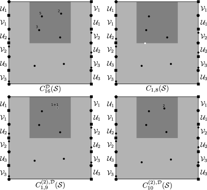
Figure 13. A configuration in each of the space introduced in Definitions 4.3 and 4.6. Whenever a multiplicity is not specified, it is equal to 1.

We have the following inclusions:

$$C_{1,m}(\mathcal{S})\subset C_{1,m}^{(2),\mathcal{D}}(\mathcal{S})\subset\mathring{\mathcal{S}}\times C_{m}^{\mathcal{D}}(\mathcal{S})\subset\mathring{\mathcal{S}}\times S\!P^{m}(\mathring{\mathcal{S}});$$

$$C_{m+1}(\mathcal{S})\subset C_{m+1}^{(2),\mathcal{D}}(\mathcal{S})\subset C_{m+1}^{\mathcal{D}}(\mathcal{S})\subset S\!P^{m+1}(\mathring{\mathcal{S}}).$$

All these spaces are manifolds of dimension $2m+2$ and all inclusions are open.

In particular there is a sequence of maps

$$H_{m+1}\left(C_{m+1}(\mathcal{S})\right)\to H_{m+1}\left(C_{m+1}^{(2),\mathcal{D}}(\mathcal{S})\right)\to H_{m+1}\left(C_{m+1}^{\mathcal{D}}(\mathcal{S})\right)$$

and we will first lift the homology class $j_{m+1}(c_{1},\dots,c_{m+1})$ to $H_{m}\left(C_{m+1}^{(2),\mathcal{D}}(\mathcal{S})\right)$ and then to $H_{m+1}(C_{m+1}(\mathcal{S}))$, each time controlling the support of our representing cycles and of the homologies between them.

Fix a neighborhood $\mathcal{N}$ of $\mathcal{D}\cup c_{1}\cup\dots\cup c_{m+1}$.

For the first lift, let $\mathcal{N}^{\prime}=\left(\mathcal{N}\setminus c_{1}\right)\cup\mathcal{D}$; note that $\mathcal{N}^{\prime}$ is open in $\mathring{\mathcal{S}}$ and contains $\mathcal{D}\cup c_{2}\cup\dots\cup c_{m+1}$, so $\mathcal{N}^{\prime}$ is an open neighborhood of $\mathcal{D}\cup c_{2}\cup\dots\cup c_{m+1}$ in $\mathring{\mathcal{S}}$. By inductive hypothesis there is a cycle $\mathfrak{c}=\tilde{\psi}_{m}(c_{2},\dots,c_{m+1})$ in $C_{m}(\mathcal{S})$ which is supported on $\mathcal{N}^{\prime}$, and such that $(\iota_{m})_{*}(\mathfrak{c})$ is homologous to $[c_{2}]\cdot\ldots\cdot[c_{m+1}]$ along a homology in $C_{m}^{\mathcal{D}}(\mathcal{S})$ supported on $\mathcal{N}^{\prime}$ as well.

We can multiply both cycles and the homology between them by the cycle $[c_{1}]$: the result are the two homologous cycles $[c_{1}]\cdot\mathfrak{c}$ and $[c_{1}]\cdot\ldots\cdot[c_{m+1}]$ in $C_{m+1}^{\mathcal{D}}(\mathcal{S})$: both cycles and the homology between them are supported on $\mathcal{N}$. Note now that the cycle $[c_{1}]\cdot\mathfrak{c}$ lives in $C_{m+1}^{(2),\mathcal{D}}(\mathcal{S})$, so the first lift is done and we can now deal with the second lift.

There is a natural map $p\colon C_{1,m}^{(2),\mathcal{D}}(\mathcal{S})\to C_{m+1}^{(2),\mathcal{D}}(\mathcal{S})$, which converts the white point into a black point. This map restricts to a map $C_{1,m}(\mathcal{S})\to C_{m+1}(\mathcal{S})$, so that we have a commutative diagram

(8) $$\begin{CD}C_{1,m}(\mathcal{S})@>{\subset}>{}>C_{1,m}^{(2),\mathcal{D}}(\mathcal{S})\\ @V{p}V{}V@V{p}V{}V\\ C_{m+1}(\mathcal{S})@>{\subset}>{}>C_{m+1}^{(2),\mathcal{D}}(\mathcal{S})\end{CD}$$

Definition 4.7.

Let

$$\triangle_{m+1}=C_{m+1}^{(2),\mathcal{D}}(\mathcal{S})\setminus C_{m+1}(\mathcal{S})$$

and similarly

$$\triangle_{1,m}=C_{1,m}^{(2),\mathcal{D}}(\mathcal{S})\setminus C_{1,m}(\mathcal{S}).$$

We note that $p$ restricts to a homeomorphism $\triangle_{1,m}\to\triangle_{m+1}$. Moreover both $\triangle_{m+1}\subset C_{m+1}^{(2),\mathcal{D}}(\mathcal{S})$ and $\triangle_{1,m}\subset C_{1,m}^{(2),\mathcal{D}}(\mathcal{S})$ are closed submanifolds of codimension $2$, and the map $p$ restricts to a $2$-fold ramified covering between their respective normal bundles.

Diagram (8) induces a commutative diagram in homology

(9) $$\begin{CD}H_{m+1}\left(C_{1,m}^{(2),\mathcal{D}}(\mathcal{S})\right)@>{}>{}>H_{m+1}\left(C_{1,m}^{(2),\mathcal{D}}(\mathcal{S}),C_{1,m}(\mathcal{S})\right)\\ @V{p_{*}}V{}V@V{p_{*}}V{}V\\ H_{m+1}\left(C_{m+1}(\mathcal{S})\right)@>{}>{}>H_{m+1}\left(C_{m+1}^{(2),\mathcal{D}}(\mathcal{S})\right)@>{}>{}>H_{m+1}\left(C_{m+1}^{(2),\mathcal{D}}(\mathcal{S}),C_{m+1}(\mathcal{S})\right)\end{CD}$$

Recall that we want to lift the homology class represented by the cycle $[c_{1}]\cdot\mathfrak{c}$ from the bottom central group to the bottom left group.

We first note that there is a lift of $[c_{1}]\cdot\mathfrak{c}$ to a cycle $[c_{1}]\otimes\mathfrak{c}$ in $\left(C_{1,m}^{(2),\mathcal{D}}(\mathcal{S})\right)$: this is defined by declaring the point in $[c_{1}]\cdot\mathfrak{c}$ that spins around $c_{1}$ to be white. We then note that the right vertical map

$$p_{*}\colon H_{m+1}\left(C_{1,m}^{(2),\mathcal{D}}(\mathcal{S}),C_{1,m}(\mathcal{S})\right)\to H_{m+1}\left(C_{m+1}^{(2),\mathcal{D}}(\mathcal{S}),C_{m+1}(\mathcal{S})\right)$$

can be rewritten, after using excision to tubular neighborhoods of $\triangle_{1,m}$ and $\triangle_{m+1}$ respectively, and the Thom isomorphism, as a map

$$H_{m-1}(\triangle_{1,m})\to H_{m-1}(\triangle_{m+1}).$$

The latter map is multiplication by $2$, after identifying $\triangle_{m+1}$ and $\triangle_{1,m}$ along $p$: indeed the normal bundle of $\triangle_{1,m}$ is a double covering of the normal bundle of $\triangle_{m+1}$, hence the Thom class of the first disc bundle corresponds to twice the Thom class of the second disc bundle. We are working with coefficients in $\mathbb{Z}_{2}$, so multiplication by $2$ is the zero map.

Therefore the image of the cycle $[c_{1}]\otimes\mathfrak{c}$ along the diagonal of the square in diagram (9) is zero; hence the image of $[c_{1}]\cdot\mathfrak{c}$ in $H_{m+1}\left(C_{m+1}^{(2),\mathcal{D}}(\mathcal{S}),C_{m+1}(\mathcal{S})\right)$ is zero; hence the homology class of $[c_{1}]\cdot\mathfrak{c}$ comes from $H_{m+1}(C_{m+1}(\mathcal{S}))$. More precisely, there exists a cycle $\mathfrak{c}^{\prime}$ in $C_{m+1}(\mathcal{S})$ such that $\left(\iota_{m+1}\right)_{*}(\mathfrak{c}^{\prime})$ is homologous to $[c_{1}]\cdot\mathfrak{c}$.

To prove Lemma 4.5 we need to find a good cycle and a good homology, namely two that are supported on $\mathcal{N}$: a priori both $\mathfrak{c}^{\prime}$ and the homology between $\left(\iota_{m+1}\right)_{*}(\mathfrak{c}^{\prime})$ and $[c_{1}]\cdot\mathfrak{c}$ are only supported on $\mathring{\mathcal{S}}$.

This can be done by replacing, in the whole argument of the proof, the surface $\mathring{\mathcal{S}}$ with the surface $\mathcal{N}$. We can define configuration spaces as in Definition 4.6 also for the open surface $\mathcal{N}$, and we can repeat the argument considering $\mathcal{N}$ as the ambient surface: indeed we only needed a surface containing $\mathcal{D}$ and all curves $c_{1},\dots,c_{m+1}$.

It is crucial that the action of $\Gamma_{g,1}$ is not involved in the statement of Lemma 4.5, as $\mathcal{N}\subset\mathcal{S}$ is not preserved, even up to isotopy, by diffeomorphisms of $\mathcal{S}$. Lemma 4.5 is proved.

We now have to prove the following lemma to conclude the proof of Theorem 3.2 in bigradings $(m,m)$.

Lemma 4.8.

The map $\tilde{\psi}_{m}\colon\mathbb{Z}_{2}\left<\mathfrak{C}^{m}\right>\to H_{m}(C_{m}(\mathcal{S}))$ is surjective and factors through the map $\mathfrak{p}_{m}$.

Proof.

The factorisation is equivalent to the inclusion $\ker\mathfrak{p}_{m}\subseteq\ker\tilde{\psi}_{m}$: since both $\mathfrak{p}_{m}$ and $\tilde{\psi}_{m}$ are $\Gamma_{g,1}$-equivariant, also the induced map of vector spaces

$$\operatorname{Sym}_{m}(\mathcal{H})=\mathbb{Z}_{2}\left<\mathfrak{C}^{m}\right>/\ker\mathfrak{p}_{m}\to H_{m}(C_{m}(\mathcal{S}))$$

will automatically be $\Gamma_{g,1}$-equivariant.

Recall from the proof of Lemma 4.4 that a basis for $\tilde{H}_{m}(C_{m}(\mathcal{S})^{\infty})$ is given by the classes $[\kappa(\underline{u},\underline{v})]$, represented by generalised symmetric chains consisting of only one tuple $\mathfrak{h}=(0,\underline{u},\underline{v})$, for some vectors $\underline{u}=(u_{1},\dots,u_{g})$ and $\underline{v}=(v_{1},\dots,v_{g})$ satisfying $\sum_{i=1}^{g}(u_{i}+v_{i})=m$.

The homology class $[\kappa(\underline{u},\underline{v})]$ is the fundamental class of the sphere $e^{\mathfrak{h}}\cup\left\{\infty\right\}\subset C_{m}(\mathcal{S})^{\infty}$: the inclusion of this sphere in $C_{m}(\mathcal{S})^{\infty}$ restricts to a proper embedding $e^{\mathfrak{h}}\subset C_{m}(\mathcal{S})$.

By Poincaré Lefschetz duality $\tilde{H}_{m}(C_{m}(\mathcal{S})^{\infty})\simeq H^{m}(C_{m}(\mathcal{S}))$, and the latter is the dual of $H_{m}(C_{m}(\mathcal{S}))$.

We can therefore associate to $[\kappa(\underline{u},\underline{v})]$ a linear functional on $H_{m}(C_{m}(\mathcal{S}))$. This is the algebraic intersection product with the cell $e^{\mathfrak{h}}$, seen as a proper submanifold of $C_{m}(\mathcal{S})$: we denote it by

$$\cdot\cap e^{\mathfrak{h}}\colon H_{m}(C_{m}(\mathcal{S}))\to\mathbb{Z}_{2}.$$

Therefore

$$\ker\tilde{\psi}_{m}=\bigcap_{\mathfrak{h}}\ker\left((\cdot\cap e^{\mathfrak{h}})\circ\tilde{\psi}_{m}\right),$$

and it suffices to check that $\ker\mathfrak{p}_{m}\subseteq\ker\left((\cdot\cap e^{\mathfrak{h}})\circ\tilde{\psi}_{m}\right)$ for all $\mathfrak{h}$ of the form $(0,\underline{u},\underline{v})$, or equivalently, that $(\cdot\cap e^{\mathfrak{h}})\circ\tilde{\psi}_{m}$ factors through $\mathfrak{p}_{m}$.

Recall from the proof of Lemma 4.4 that the cohomology class $(\cdot\cap e^{\mathfrak{h}})$ on $C_{m}(\mathcal{S})$ is a pullback of a cohomology class of $C_{m}^{\mathcal{D}}(\mathcal{S})$, that we call $(\cdot\cap e^{\mathfrak{h}})^{\mathcal{D}}$. Alternatively, note that the inclusion $e^{\mathfrak{h}}\cap\left\{\infty\right\}\to C_{m}(\mathcal{S})^{\infty}$ is the composition of the inclusion $e^{\mathfrak{h}}\cap\left\{\infty\right\}\to C_{m}^{\mathcal{D}}(\mathcal{S})^{\infty}$ and the quotient map $C_{m}^{\mathcal{D}}(\mathcal{S})^{\infty}\to C_{m}(\mathcal{S})^{\infty}$, and consider the fundamental class of the sphere $e^{\mathfrak{h}}\cup\left\{\infty\right\}$ and its images.

We can therefore compute the map $(\cdot\cap e^{\mathfrak{h}})\circ\tilde{\psi}_{m}$ as the map

(10) $$(\cdot\cap e^{\mathfrak{h}})^{\mathcal{D}}\circ j_{m}\colon\mathbb{Z}_{2}\left<\mathfrak{C}^{m}\right>\to\mathbb{Z}_{2}.$$

The latter map coincides with the composition

(11) $$\left(\prod_{i=1}^{g}(\cdot\cap\mathcal{U}_{i})^{u_{i}}(\cdot\cap\mathcal{V}_{i})^{v_{i}}\right)\circ\mathfrak{p}_{m},$$

where $\prod_{i=1}^{g}(\cdot\cap\mathcal{U}_{i})^{u_{i}}(\cdot\cap\mathcal{V}_{i})^{v_{i}}\in\operatorname{Sym}_{m}(\operatorname{Hom}(\mathcal{H};\mathbb{Z}_{2}))=\operatorname{Hom}\left(\operatorname{Sym}_{m}(\mathcal{H});\mathbb{Z}_{2}\right)$.

This can be checked on every generator $(c_{1},\dots,c_{m})\in\mathbb{Z}_{2}\left<\mathfrak{C}^{m}\right>$ by chosing in the isotopy class a representative $(c_{1},\dots,c_{m})$ with all curves $c_{i}$ transverse to all segments $\mathcal{U}_{j}$ and $\mathcal{V}_{j}$.

Consider again the map $c_{1}\times\dots\times c_{m}\colon\left(\mathbb{S}^{1}\right)^{\times m}\to C_{m}^{\mathcal{D}}(\mathcal{S})$ that we used to define the cycle $[c_{1}]\cdot\dots[c_{m}]$ representing the class $j_{m}(c_{1},\dots,c_{m})$ (see Definition 4.3): this map is an embedding near $e^{\mathfrak{h}}$ and is transverse to $e^{\mathfrak{h}}$.

The equality of the maps in equations (10) and (11) on the generator $(c_{1},\dots,c_{m})\in\mathbb{Z}_{2}\left<\mathfrak{C}^{m}\right>$ follows from a straightforward computation (in $\mathbb{Z}_{2}$) of the cardinality of the set $[c_{1}]\cdot\dots[c_{m}]\cap e^{\mathfrak{h}}$ in terms of the cardinalities of all sets of the form $c_{i}\cap\mathcal{U}_{j}$ and $c_{i}\cap\mathcal{V}_{j}$. In particular $(\cdot\cap e^{\mathfrak{h}})\circ\tilde{\psi}_{m}$ factors through $\mathfrak{p}_{m}$.

To show surjectivity of $\tilde{\psi}_{m}$, choose a tuple $\mathfrak{h}$ of the form $(0,\underline{u},\underline{v})$ and an $m$-tuple of curves $(c_{1},\dots,c_{m})$ containing, for every $1\leq i\leq g$, $u_{i}$ parallel copies of some curve representing $\mathfrak{u}_{i}$ and $v_{i}$ parallel copies of some curve representing $\mathfrak{v}_{i}$ (see Definition 3.9), such that all intersections between these curves lie in $\mathcal{D}$.

Then $j_{m}(c_{1},\dots,c_{m})\cap e^{\mathfrak{h}}=1$ and for all other tuples $\mathfrak{h}^{\prime}$ of the form $(0,\underline{u}^{\prime},\underline{v})$ we have instead $j_{m}(c_{1},\dots,c_{m})\cap e^{\mathfrak{h}^{\prime}}=0$.

This shows that $\psi_{m}(c_{1},\dots,c_{m})=[c_{1}]\cdot\ldots\cdot[c_{m}]\in\operatorname{Sym}_{m}(\mathcal{H})$, which is one of the generating monomials. ∎

Theorem 3.2 is now proved in all bigradings of the form $(m,m)$.

4.3. General bigradings $(m-l,m)$.

Fix $0\leq l\leq m$ for the whole subsection: our next aim is to prove Theorem 3.2 for the bigrading $(m-l,m)$.

For all $0\leq p\leq m$, the group $\operatorname{Diff}(\mathcal{S};\partial\mathcal{S}\cup\mathcal{D})$ acts both on $C_{p}(\mathcal{D})\times C_{m-p}(\mathcal{S}^{\prime})$ and on $C_{m}(\mathcal{S})$, and the map $\mu$ is equivariant with respect to this action (see Definition 2.3); hence, using the Künneth formula, there is an induced $\Gamma_{g,1}$-equivariant map in homology

(12) $$\mu_{*}\colon H_{p-l}\left(C_{p}(\mathcal{D})\right)\otimes H_{m-p}\left(C_{m-p}(\mathcal{S}^{\prime})\right)\to H_{m-l}\left(C_{m}(\mathcal{S})\right).$$

Note that $H_{p-l}\left(C_{p}(\mathcal{D})\right)\otimes H_{m-p}\left(C_{m-p}(\mathcal{S}^{\prime})\right)$ is the tensor product of the trivial representation $H_{p-l}\left(C_{p}(\mathcal{D})\right)$, and of the representation $H_{m-p}\left(C_{m-p}(\mathcal{S}^{\prime})\right)$, which by the results of the previous section is isomorphic to the symplectic representation $\operatorname{Sym}_{m-p}(\mathcal{H})$.

We will prove the following lemma, from which Theorem 3.2 follows:

Lemma 4.9.

For all $l\leq p\leq m$ the map $\mu_{*}$ in equation (12) is injective, and the collection of all these maps yields a splitting

(13) $$H_{m-l}(C_{m}(\mathcal{S}))=\bigoplus_{p=l}^{m}H_{p-l}\left(C_{p}(\mathcal{D})\right)\otimes H_{m-p}\left(C_{m-p}(\mathcal{S}^{\prime})\right).$$

Proof.

Note that the statement of the lemma does not depend on the the action of $\Gamma_{g,1}$: we have a map from the right-hand side to the left-hand side of equation (13), we already know that it is $\Gamma_{g,1}$-equivariant, we only need to show that it is a linear isomorphism. Note also that Lemma 3.8 implies that the two vector spaces have the same dimension.

Fix $l\leq p\leq m$ and $\underline{\alpha}=(\alpha_{j})_{j\geq 0}$, and let $[a]=Q^{\underline{\alpha}}\varepsilon=\prod_{j=0}^{\infty}(Q^{j}\varepsilon)^{\alpha_{j}}$ be a generator of $H_{p-l}(C_{p}(\mathcal{D}))$, hence $l=\sum_{j}\alpha_{j}$ and $p=\sum_{j}\alpha_{j}2^{j}$.

Fix also $\underline{u}=(u_{1},\dots,u_{g})$ and $\underline{v}=(v_{1},\dots,v_{g})$, and let $[b]=\mathfrak{u}^{\underline{u}}\cdot\mathfrak{v}^{\underline{v}}=\prod_{i=1}^{g}(\mathfrak{u}_{i}^{u_{i}}\mathfrak{v}_{i}^{v_{i}})$ be a generator of $H_{m-p}(C_{m-p}(\mathcal{S}^{\prime}))$, using the isomorphism proved in the previous subsection, with $(m-p)=\sum_{i}(u_{i}+v_{i})$.

Here $a$ and $b$ are chosen singular cycles representing the homology classes, with $a$ supported on $\mathcal{D}$ and $b$ supported on $\mathcal{S}^{\prime}$. See Figure 14

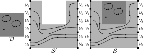
Figure 14. From left to right, the class $[a]=\varepsilon\cdot(Q\varepsilon)^{2}\in H_{2}(C_{5}(\mathcal{D}))$; the class $[b]=\mathfrak{v}_{1}\cdot\mathfrak{u}_{2}\cdot\mathfrak{v}_{3}^{2}\in H_{4}(C_{4}(\mathcal{S}^{\prime}))$; and the product class $\mu_{*}([a]\otimes[b])\in H_{6}(C_{9}(\mathcal{S}))$.

Then $[a]\otimes[b]$ is a generator of $H_{p-l}(C_{p}(\mathcal{D}))\otimes H_{m-p}(C_{m-p}(\mathcal{S}^{\prime}))$, by the Künneth formula, and we are interested in the homology class $\mu_{*}([a]\otimes[b])$.

There is one such class for any choice of $[a]$ and $[b]$ as above, that is, for any choice of $p$, $\underline{\alpha}$, $\underline{u}$ and $\underline{v}$ satisfying the conditions $l=\sum_{j\geq 0}\alpha_{j}$, $p=\sum_{j\geq 0}\alpha_{j}2^{j}$ and $(m-p)=\sum_{i=1}^{g}(u_{i}+v_{i})$, where we use the notation above.

We want to show that the collection of all the corresponding classes of the form $\mu_{*}([a]\otimes[b])$ gives a basis for $H_{m-l}(C_{m}(\mathcal{S}))$.

We will study the intersection of $\mu_{*}([a]\otimes[b])$ with cohomology classes of $C_{m}(\mathcal{S})$ represented by generalised symmetric chains in $C_{m}(\mathcal{S})^{\infty}$.

To compute the algebraic intersection between $\mu_{*}([a]\otimes[b])$ and $[\kappa(p^{\prime},\underline{\alpha}^{\prime},\underline{u}^{\prime},\underline{v}^{\prime})]$ we consider the map

$$\mu^{\infty}\colon C_{m}(\mathcal{S})^{\infty}\to\left(C_{p}(\mathcal{D})\times C_{m-p}(\mathcal{S}^{\prime})\right)^{\infty}$$

which collapses to $\infty$ the complement in $C_{m}(\mathcal{S})^{\infty}$ of the open submanifold $C_{p}(\mathcal{D})\times C_{m-p}(\mathcal{S}^{\prime})$.

By Poincaré-Lefschetz duality, the map $\mu^{\infty}_{*}$ in reduced homology corresponds to the cohomology map

$$\mu^{*}\colon H^{*}(C_{m}(\mathcal{S}))\to H^{*}(C_{p}(\mathcal{D})\times C_{m-p}(\mathcal{S}^{\prime}))=H^{*}(C_{p}(\mathcal{D}))\otimes H^{*}(C_{m-p}(\mathcal{S}^{\prime})).$$

We give $\left(C_{p}(\mathcal{D})\times C_{m-p}(\mathcal{S}^{\prime})\right)^{\infty}$ the cell complex structure of the smash product $C_{p}(\mathcal{D})^{\infty}\wedge C_{m-p}(\mathcal{S}^{\prime})^{\infty}$. Here $C_{p}(\mathcal{D})^{\infty}$ is given the cell structure of $C_{p}((0,1)^{2})^{\infty}$ coming from the natural identification $\mathcal{D}=]1/4,3/4[\times]1/2,1[\cong]0,1[^{2}$, which is obtained by rescaling and translating. Moreover we choose any diffeomorphism $\mathring{\mathcal{S}}^{\prime}\cong\mathring{\mathcal{S}}$ that restricts to the identity on all $\mathcal{U}_{i}$’s and $\mathcal{V}_{i}$’s, and give $C_{m-p}(\mathcal{S}^{\prime})^{\infty}$ the cell structure of $C_{m-p}(\mathcal{S})^{\infty}$.

Recall that $C_{m}(\mathcal{S})^{\infty}$ can be filtered according to the norm of cells: a cell $e^{\mathfrak{h}}$ associated with the tuple $\mathfrak{h}=(l,\underline{x},\underline{u},\underline{v})$ has norm $\sum_{i=1}^{l}x_{i}$, and the norm is weakly decreasing along boundaries. In the previous section we just considered the associated filtration of the reduced chain complex $\tilde{\mathcal{C}}_{*}(C_{m}(\mathcal{S})^{\infty})$, whereas now we consider the closed subcomplex $F_{p}C_{m}(\mathcal{S})^{\infty}\subset C_{m}(\mathcal{S})^{\infty}$, which is the union of all cells of norm $\leq p$.

The crucial observation is that $\mu^{\infty}$ restricts to a cellular map

$$F_{p}C_{m}(\mathcal{S})^{\infty}\to\left(C_{p}(\mathcal{D})\times C_{m-p}(\mathcal{S}^{\prime})\right)^{\infty}.$$

To see this, fix a tuple $\tilde{\mathfrak{h}}=(\tilde{l},\tilde{\underline{x}},\tilde{\underline{u}},\tilde{\underline{v}})$ of norm $\tilde{p}\leq p$ and of dimension $\tilde{l}+m$, and consider the open cell cell $e^{\tilde{\mathfrak{h}}}\subset F_{p}C_{m}(\mathcal{S})^{\infty}$.

If $\tilde{p}<p$, then $e^{\tilde{\mathfrak{h}}}\cap(C_{p}(\mathcal{D})\times C_{m-p}(\mathcal{S}^{\prime}))$ is empty. If $\tilde{p}=p$, then

$$e^{\tilde{\mathfrak{h}}}\cap(C_{p}(\mathcal{D})\times C_{m-p}(\mathcal{S}^{\prime}))=e^{\mathfrak{h}^{\prime}}\times e^{\mathfrak{h}^{\prime\prime}},$$

where $\mathfrak{h}^{\prime}=(\tilde{l},\tilde{\underline{x}})$ and $\mathfrak{h}^{\prime\prime}=(0,\tilde{\underline{u}},\tilde{\underline{v}})$.

Therefore $\mu^{\infty}(e^{\tilde{\mathfrak{h}}})$ is $\left\{\infty\right\}$ in the first case, and in the second case it is contained in the union $\left\{\infty\right\}\cup e^{\mathfrak{h}^{\prime}}\times e^{\mathfrak{h}^{\prime\prime}}$, which is also contained in the $(\tilde{l}+m)$-skeleton of $\left(C_{p}(\mathcal{D})\times C_{m-p}(\mathcal{S}^{\prime})\right)^{\infty}$.

Consider now the generalised symmetric chain $\kappa(p^{\prime},\underline{\alpha}^{\prime},\underline{u}^{\prime},\underline{v}^{\prime})$ representing a class in $\tilde{H}_{m+l}(C_{m}(\mathcal{S})^{\infty})=H^{m-l}(C_{m}(\mathcal{S}))$, with $\underline{\alpha}^{\prime}=(\alpha^{\prime}_{j})_{j\geq 0}$, $\underline{u}^{\prime}=(u_{1},\dots,u^{\prime}_{g})$ and $\underline{v}^{\prime}=(v^{\prime}_{1},\dots,v^{\prime}_{g})$; in particular $l=\sum_{j\geq 0}\alpha^{\prime}_{j}$. Suppose moreover $p^{\prime}\leq p$.

If $p^{\prime}<p$, the previous argument shows that $\mu^{\infty}_{*}\left(\kappa(p^{\prime},\underline{\alpha}^{\prime},\underline{u}^{\prime},\underline{v}^{\prime})\right)=0$ in the reduced cellular chain complex, and in particular the corresponding homology class is mapped to zero.

Suppose now $p^{\prime}=p$: then the previous argument shows that the homology class $[\kappa(p^{\prime},\underline{\alpha}^{\prime},\underline{u}^{\prime},\underline{v}^{\prime})]\in\tilde{H}_{m+l}(C_{m}(\mathcal{S})^{\infty})$ is mapped along $\mu^{\infty}_{*}$ to the class

$$[\kappa(\underline{\alpha}^{\prime})]\otimes[\kappa(\underline{u}^{\prime},\underline{v}^{\prime})]\in\tilde{H}\left(C_{p}(\mathcal{D})^{\infty}\wedge C_{m-p}(\mathcal{S}^{\prime})^{\infty}\right).$$

Indeed each tuple $\mathfrak{h}$ in the cycle $\kappa(p^{\prime},\underline{\alpha}^{\prime},\underline{u}^{\prime},\underline{v}^{\prime})|$ is mapped by $\mu^{\infty}_{*}$ to a corresponding pair of tuples $\mathfrak{h}^{\prime}\otimes\mathfrak{h}^{\prime\prime}$ in the cycle $\kappa(\underline{\alpha}^{\prime})\otimes\kappa(\underline{u}^{\prime},\underline{v}^{\prime})$, so even at the level of chains we have

$$\mu^{\infty}_{*}\left(\kappa(p^{\prime},\underline{\alpha}^{\prime},\underline{u}^{\prime},\underline{v}^{\prime})\right)=\kappa(\underline{\alpha}^{\prime})\otimes\kappa(\underline{u}^{\prime},\underline{v}^{\prime}).$$

We can now compute the algebraic intersection of $\mu_{*}([a]\otimes[b])$ with the cohomology class $[\kappa(p^{\prime},\underline{\alpha}^{\prime},\underline{u}^{\prime},\underline{v}^{\prime})]$ as the algebraic intersection between $[a]\otimes[b]$ and $\mu^{\infty}_{*}\left([\kappa(p^{\prime},\underline{\alpha}^{\prime},\underline{u}^{\prime},\underline{v}^{\prime})]\right)$.

For $p^{\prime}<p$ the previous argument show that this intersection is zero.

For $p^{\prime}=p$ the intersection between $[a]\otimes[b]$ and $\mu^{\infty}_{*}([\kappa(p,\underline{\alpha}^{\prime},\underline{u}^{\prime},\underline{v}^{\prime})])=[\kappa(\underline{\alpha}^{\prime})]\otimes[\kappa(\underline{u}^{\prime},\underline{v}^{\prime})]$ is $1\in\mathbb{Z}_{2}$ exactly when $\underline{\alpha}=\underline{\alpha}^{\prime}$, $\underline{u}=\underline{u}^{\prime}$ and $\underline{v}=\underline{v}^{\prime}$; otherwise it is $0$.

To finish the proof we consider the collection of all strings of the form

$$\left(p,\underline{\alpha}=(\alpha_{j})_{j\geq 0},\underline{u}=(u_{1},\dots,u_{g}),\underline{v}=(v_{1},\dots,v_{g})\right)$$

satisfying $l=\sum_{j}\alpha_{j}$,$p=\sum_{j}\alpha_{j}2^{j}$ and $(m-p)=\sum_{i}(u_{i}+v_{i})$; we choose a total order on the set of these strings, such that the parameter $p$ is weakly increasing along this order; we associate to each string its corresponding class in $H_{m-l}(C_{m}(\mathcal{S}))$ of the form $\mu_{*}([a]\otimes[b])$ and its corresponding class $[\kappa(p,\underline{\alpha}^{\prime},\underline{u}^{\prime},\underline{v}^{\prime})]\in\tilde{H}_{m+l}(C_{m}(\mathcal{S})^{\infty})$.

Then the matrix of algebraic intersections between these two sets of classes is an upper-triangular matrix with $1$’s on the diagonal, and in particular it is invertible. This shows that the set of classes of the form $\mu_{*}([a]\otimes[b])$ is a basis for $H_{m-l}(C_{m}(\mathcal{S}))$. ∎

One could expect that the basis given by classes of the form $[a]\otimes[b]\in H_{m-l}(C_{m}(\mathcal{S}))$ is also dual to the basis of classes $[\kappa(p,\underline{\alpha},\underline{u},\underline{v})]\in\tilde{H}_{m+l}(C_{m}(\mathcal{S})^{\infty})$, i.e., the matrix considered in the end of the previous proof is not only upper-triangular but also diagonal. This is however not true, as the following example shows.

Let $g=1$, $m=2$, $p=1$, $p^{\prime}=2$ and consider the classes $[a]=\varepsilon\in H_{0}(C_{1}(\mathcal{D}))$, $[b]=\mathfrak{u}_{1}\in\mathcal{H}=H_{1}(C_{1}(\mathcal{S}^{\prime}))$. Moreover let the generalised symmetric chain $\kappa(p^{\prime},\underline{\alpha}^{\prime},\underline{u}^{\prime},\underline{v}^{\prime})$ be defined by $\underline{\alpha}^{\prime}=(\alpha^{\prime}_{j})_{j\geq 0}$ with $\alpha^{\prime}_{1}=1$ and all other $\alpha_{j}=0$, $\underline{u}^{\prime}=(u^{\prime}_{1}=0)$ and $\underline{v}^{\prime}=(v^{\prime}_{1}=0)$.

Represent $[a]$ by a point in $a\in\mathcal{D}$, for example the point $(1/2,3/4)$; represent $[b]$ by a simple closed curve $b\subset\mathcal{S}^{\prime}$ that intersects only once, transversely, the vertical segment passing through $a$, i.e. $\left\{1/2\right\}\times]0,1[$. See Figure 15.

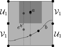
Figure 15. $\mu_{*}(a\otimes b)$ and $e^{\mathfrak{h}^{\prime}}$ intersect once, transversely inside $C_{2}(\mathcal{S})$.

Then the cycle $\kappa(p^{\prime},\underline{\alpha}^{\prime},\underline{u}^{\prime},\underline{v}^{\prime})$ consists uniquely of one tuple

$$\mathfrak{h}^{\prime}=(1,\underline{x}^{\prime}=(x^{\prime}_{1}=2),\underline{u}^{\prime}=(u^{\prime}_{1}=0),\underline{v}^{\prime}=(v^{\prime}_{1}=0)).$$

The corresponding cell $e^{\mathfrak{h}^{\prime}}$ intersects once, transversely, the cycle $\mu_{*}(a\otimes b)$, which is represented by the curve of configurations of two points in $\mathring{\mathcal{S}}$, one of which is fixed at $a$ whereas the other runs along $b$: there is exactly one position on $b$ lying under $a$.

Hence the algebraic intersection between these two classes is $1$, and since $p^{\prime}>p$ this is an entry strictly above the diagonal in the matrix considered in the proof of Lemma 4.9.

The proof of Theorem 3.2 can be easily generalised to surfaces with more than one boundary curve. Let $\Sigma_{g,n}$ be a surface of genus $g$ with $n\geq 1$ parametrised boundary curves and let $\Gamma_{g,n}$ be the group of connected components of the topological group $\operatorname{Diff}(\Sigma_{g,n};\partial\Sigma_{g,n})$: then there is an isomorphism of bigraded $\mathbb{Z}_{2}$-representations

(14) $$\bigoplus_{m\geq 0}H_{*}\left(C_{m}(\Sigma_{g,n})\right)\simeq\mathbb{Z}_{2}\left[Q^{j}\varepsilon\,|\,j\geq 0\right]\otimes\operatorname{Sym}_{\bullet}(H_{1}(\Sigma_{g,n})),$$

where the action of $\Gamma_{g,n}$ on the right-hand side is induced by the natural action on $H_{1}(\Sigma_{g,n})$.

For $n\geq 2$ the intersection form on the vector space $H_{1}(\Sigma_{g,n})$ is degenerate, but it is still invariant under the action of $\Gamma_{g,n}$, so there is still a map from $\Gamma_{g,n}$ to the subgroup of $GL_{2g+n-1}(\mathbb{Z}_{2})$ fixing this bilinear form, and in this sense we can say that the representation in (14) is symplectic.

The proof of the isomorphism (14) is almost verbatim the same; the main difference is in the construction of the model $\mathcal{T}(\Sigma_{g,n})$ for $\mathring{\Sigma}_{g,n}$: we divide the vertical segments $\left\{0,1\right\}\times[0,1]\subset[0,1]^{2}$ into $2g+n-1$ equal parts, that we call $I_{i}^{l}$ and $I_{i}^{r}$ according to their order; we identify, for each $i>2g$, the interval $I_{i}^{l}$ with the interval $I_{i}^{r}$; the other couples of intervals, yielding the genus, are identified just as before.

One can further generalise to non-orientable surfaces with non-empty boundary: it suffices, in the above construction, to glue some of the intervals $I_{i}^{l}$ and $I_{i}^{r}$ reversing their orientation. We leave all details of these generalisations to the interested reader.

5. Proof of Theorem 1.1

We will prove Theorem 1.1 by induction on $m$. The case $m=0$ is trivial.

For all $m\geq 0$ we let $E(m)$ be the Leray-Serre spectral sequence associated with the bundle (4): its second page has the form

$$E(m)^{2}_{k,q}=H_{k}(B\operatorname{Diff}(\mathcal{S};\partial\mathcal{S}\cup\mathcal{D});H_{q}(C_{m}(\mathcal{S})))=H_{k}(\Gamma_{g,1};H_{q}(C_{m}(\mathcal{S}))).$$

From Theorem 3.2 we know that this spectral sequence is concentrated on the rows $q=0,\dots,m$.

We want to prove the vanishing of all differentials appearing in the pages $E(m)^{r}$ with $r\geq 2$; the $r$-th differential takes the form

$$\partial_{r}\colon E(m)^{r}_{k,q}\to E(m)^{r}_{k-r,q+r-1}.$$

In particular any differential $\partial_{r}$ exiting from the row $q=m$ is trivial, because it lands in a higher, hence trivial row.

Fix now $q=m-l<m$, in particular $l\geq 1$; by Theorem 3.2, and in particular by Lemma 4.9, we have a splitting of $H_{k}(\Gamma_{g,1};H_{m-l}(C_{m}(\mathcal{S})))$ as

(15) $$\bigoplus_{p=l}^{m}H_{k}\left(\Gamma_{g,1};\mu_{*}\left(H_{p-l}(C_{p}(\mathcal{D}))\otimes H_{m-p}(C_{m-p}(\mathcal{S}^{\prime}))\right)\right).$$

We fix now $l\leq p\leq m$ and show the vanishing of all differentials $\partial_{r}$ exiting from the summand with label $p$ in the previous equation.

Consider the map $\mu^{\mathcal{F}}$ from Definition 2.4 as a map of bundles over the space $B\operatorname{Diff}(\mathcal{S};\partial\mathcal{S}\cup\mathcal{D})$:

$$\mu^{\mathcal{F}}\colon C_{p}(\mathcal{D})\times C_{m-p}(\mathcal{F}_{\mathcal{S}^{\prime}})\to C_{m}(\mathcal{F}_{\mathcal{S},\mathcal{D}}).$$

Note that the first bundle $C_{p}(\mathcal{D})\times C_{m-p}(\mathcal{F}_{\mathcal{S}^{\prime}})\to B\operatorname{Diff}(\mathcal{S};\partial\mathcal{S}\cup\mathcal{D})$ is the product of the space $C_{p}(\mathcal{D})$ with the bundle $C_{m-p}(\mathcal{F}_{\mathcal{S}^{\prime}})\to B\operatorname{Diff}(\mathcal{S};\partial\mathcal{S}\cup\mathcal{D})$; therefore the spectral sequence associated with $C_{p}(\mathcal{D})\times C_{m-p}(\mathcal{F}_{\mathcal{S}^{\prime}})$ is isomorphic, from the second page on, to the tensor product of $H_{*}(C_{p}(\mathcal{D}))$ and the spectral sequence associated with the bundle $C_{m-p}(\mathcal{F}_{\mathcal{S}^{\prime}})$; the latter spectral sequence is isomorphic, in our notation, to the spectral sequence $E(m-p)$. In particular $\mu^{\mathcal{F}}$ induces a map of spectral sequences

$$\mu^{\mathcal{F}}_{*}\colon H_{*}(C_{p}(\mathcal{D}))\otimes E(m-p)\to E(m);$$

that in the second page, on the $(m-l)$-th row and $k$-th column, restricts to the inclusion of one of the direct summands in equation (15):

$$H_{k}\left(\Gamma_{g,1};\mu_{*}(H_{p-l}(C_{p}(\mathcal{D}))\otimes H_{m-p}(C_{m-p}(\mathcal{S}^{\prime})))\right)\subset H_{k}\left(\Gamma_{g,1};H_{m-l}(C_{m}(\mathcal{S}))\right).$$

In particular if we prove the vanishing of all differentials $\partial_{r}$ in the first spectral sequence, then also all differentials $\partial_{r}$ exiting from this direct summand in the second spectral sequence $E(m)$ must vanish.

The differentials in the spectral sequence $H_{*}(C_{p}(\mathcal{D}))\otimes E(m-p)$ are obtained by tensoring the identity of $H_{*}(C_{p}(\mathcal{D}))$ with the differentials of the spectral sequence $E(m-p)$; as $p\geq l\geq 1$ we know by inductive hypothesis that the latter vanish. Theorem 1.1 is proved.

One can generalise Theorem 1.1 to orientable or non-orientable surfaces with non-empty boundary, following the generalisation of Theorem 3.2 discussed at the end of Section 4.

6. Comparison with the work of Bödigheimer and Tillmann

In this section we will compare Theorems 1.1 and 3.2 with the results in [4]. In particular we consider the following two theorems, that we formulate in an equivalent, but different way as in [4], fitting in our framework. In the entire section homology is taken with coefficients in $\mathbb{Z}_{2}$ unless explicitly stated otherwise.

Theorem 6.1 (Corollary 1.2 in [4]).

Let $\mathbb{F}$ be a field, and let $m\geq 0$, $g\geq 0$. Then the following graded vector spaces are isomorphic in degrees $*\leq\frac{2}{3}g-\frac{2}{3}$

$$H_{*}\left(\Gamma_{g,1}^{m};\mathbb{F}\right)\cong H_{*}\left(\Gamma_{g,1};\mathbb{F}\right)\otimes_{\mathbb{F}}H_{*}\left(\mathfrak{S}_{m};\mathbb{F}[x_{1},\dots,x_{m}]\right).$$

Here each variable $x_{1},\dots,x_{m}$ has degree 2 and the symmetric group $\mathfrak{S}_{m}$ acts on the polynomial ring $\mathbb{F}[x_{1},\dots,x_{m}]$ by permuting the variables.

We point out that the range of degrees $*\leq\frac{2}{3}g-\frac{2}{3}$ is the stable range for the homology $H_{*}(\Gamma_{g,1};\mathbb{F})$ of the mapping class group, see [11] for the original stability theorem and [5, 15] for the improved stability range.

Theorem 6.2 (Theorem 1.3 in [4]).

For all $m\geq 0$ the map $\mu^{\mathcal{F}}\colon C_{1}(\mathcal{D})\times C_{m}(\mathcal{F}_{\mathcal{S}^{\prime}})\to C_{m+1}(\mathcal{F}_{\mathcal{S},\mathcal{D}})$ from Definition 2.4 induces a split-injective map in homology

$$\mu^{\mathcal{F}}_{*}\colon H_{*}\left(C_{m}(\mathcal{F}_{\mathcal{S}^{\prime}})\right)\cong H_{0}\left(C_{1}(\mathcal{D})\right)\otimes_{\mathbb{F}}H_{*}\left(C_{m}(\mathcal{F}_{\mathcal{S}^{\prime}})\right)\hookrightarrow H_{*}\left(C_{m+1}(\mathcal{F}_{\mathcal{S},\mathcal{D}})\right).$$

In other words, the inclusion of groups $\Gamma_{g,1}^{m}\hookrightarrow\Gamma_{g,1}^{m+1}$ given by adding a puncture near the boundary induces a split injective map $H_{*}(\Gamma_{g,1}^{m};\mathbb{F})\hookrightarrow H_{*}(\Gamma_{g,1}^{m+1};\mathbb{F})$.

We first reformulate Theorems 1.1 and 3.2 in a convenient way.

Definition 6.3.

We introduce some abbreviations for the following disjoint unions:

$$C_{\bullet}(\mathcal{D})=\coprod_{m\geq 0}C_{m}(\mathcal{D});$$

$$C_{\bullet}(\mathcal{S})=\coprod_{m\geq 0}C_{m}(\mathcal{S});$$

$$C_{\bullet}(\mathcal{F}_{\mathcal{S},\mathcal{D}})=\coprod_{m\geq 0}C_{m}(\mathcal{F}_{\mathcal{S},\mathcal{D}}).$$

Then $C_{\bullet}(\mathcal{D})$ is a (homotopy associative) topological monoid, with associated Pontryagin ring $H_{*}\left(C_{\bullet}(\mathcal{D})\right)\cong\mathbb{Z}_{2}[Q^{j}\varepsilon|j\geq 0]$ (see Equation 5). This is a bigraded ring, where the two gradings are the homological degree and the weight.

The maps $\mu$ from Definition 2.4 make $C_{\bullet}(\mathcal{S})$ into a (homotopy associative) module over the monoid $C_{\bullet}(\mathcal{D})$; correspondingly $H_{*}\left(C_{\bullet}(\mathcal{S})\right)$ is a bigraded module over $H_{*}\left(C_{\bullet}(\mathcal{D})\right)$. The structure of this module is described by the following reformulation of Theorem 3.2, see in particular the proof of Lemma 4.9.

Theorem 6.4.

There is an isomorphism of $\Gamma_{g,1}$-representations in (bigraded) modules over the ring $H_{*}\left(C_{\bullet}(\mathcal{D})\right)$

$$H_{*}\left(C_{\bullet}(\mathcal{S})\right)\cong H_{*}\left(C_{\bullet}(\mathcal{D})\right)\otimes\operatorname{Sym}_{\bullet}(\mathcal{H}).$$

Similarly, Theorem 1.1 can be reformulated as follows, considering at the same time all values of $m\geq 0$.

Theorem 6.5.

There is an isomorphism of (bigraded) modules over $H_{*}\left(C_{\bullet}(\mathcal{D})\right)$

$$H_{*}\left(C_{\bullet}(\mathcal{F}_{\mathcal{S},\mathcal{D}})\right)\cong H_{*}\left(C_{\bullet}(\mathcal{D})\right)\otimes H_{*}\left(\Gamma_{g,1};\operatorname{Sym}_{\bullet}(\mathcal{H})\right).$$

The proof follows from the arguments used in Section 5: we have actually shown that the direct sum of the spectral sequences $\bigoplus_{m\geq 0}E(m)$ is itself a free module over $H_{*}\left(C_{\bullet}(\mathcal{D})\right)$ on the second page, with the same description as above.

By virtue of homological stability in $g$ for the sequences of groups $\left(\Gamma_{g,1}\right)_{g\geq 0}$ and $\left(\Gamma_{g,1}^{m}\right)_{g\geq 0}$, Theorem 6.1 can be equivalently rephrased as an isomorphism of graded vector spaces

$$H_{*}\left(\Gamma_{\infty,1}^{m};\mathbb{F}\right)\cong H_{*}\left(\Gamma_{\infty,1};\mathbb{F}\right)\otimes_{\mathbb{F}}H_{*}\left(\mathfrak{S}_{m};\mathbb{F}[x_{1},\dots,x_{m}]\right).$$

Here $\Gamma_{\infty,1}=\mathop{\mathrm{colim}}\nolimits_{g\to\infty}\Gamma_{g,1}$ and $\Gamma_{\infty,1}^{m}=\mathop{\mathrm{colim}}\nolimits_{g\to\infty}\Gamma_{g,1}^{m}$.

Let $\Gamma_{\infty,1}^{\bullet}$ denote the disjoint union $\coprod_{m\geq 0}\Gamma_{\infty,1}^{m}$, which we consider as a groupoid. Then Theorem 6.1 is equivalent to the isomorphism of bigraded vector spaces

$$H_{*}\left(\Gamma_{\infty,1}^{\bullet};\mathbb{F}\right)\cong H_{*}\left(\Gamma_{\infty,1};\mathbb{F}\right)\otimes_{\mathbb{F}}\left(\bigoplus_{m\geq 0}H_{*}\left(\mathfrak{S}_{m};\mathbb{F}[x_{1},\dots,x_{m}]\right)\right).$$

We consider $\bigoplus_{m\geq 0}H_{*}\left(\mathfrak{S}_{m};\mathbb{F}[x_{1},\dots,x_{m}]\right)$ as a free module over the Pontryagin ring $H_{*}(\mathfrak{S}_{\bullet};\mathbb{F})$, where $\mathfrak{S}_{\bullet}=\coprod_{m\geq 0}\mathfrak{S}_{m}$ and the Pontryagin product is induced by the natural maps of groups $\mathfrak{S}_{m}\times\mathfrak{S}_{m^{\prime}}\to\mathfrak{S}_{m+m^{\prime}}$. This module structure is induced by the natural maps

$$H_{*}\left(\mathfrak{S}_{m};\mathbb{F}[x_{1},\dots,x_{m}]\right)\otimes_{\mathbb{F}}H_{*}\left(\mathfrak{S}_{m^{\prime}};\mathbb{F}\right)\to H_{*}\left(\mathfrak{S}_{m}\times\mathfrak{S}_{m^{\prime}};\mathbb{F}[x_{1},\dots,x_{m}]\otimes_{\mathbb{F}}\mathbb{F}\right)\to$$

$$\to H_{*}\left(\mathfrak{S}_{m+m^{\prime}};\mathbb{F}[x_{1},\dots,x_{m+m^{\prime}}]\right),$$

where the first arrow is given by the homology cross product and the second by the aforementioned inclusion $\mathfrak{S}_{m}\times\mathfrak{S}_{m^{\prime}}\to\mathfrak{S}_{m+m^{\prime}}$ together with the (equivariant) inclusion of coefficients

$$\mathbb{F}[x_{1},\dots,x_{m}]\otimes_{\mathbb{F}}\mathbb{F}=\mathbb{F}[x_{1},\dots,x_{m}]\subset\mathbb{F}[x_{1},\dots,x_{m+m^{\prime}}].$$

From now on we assume $\mathbb{F}=\mathbb{Z}_{2}$. Let $\beta_{m}=\beta_{m}(\mathcal{D})$ denote the braid group on $m$ strands of the disc, and let $\beta_{\bullet}=\coprod_{m\geq 0}\beta_{m}$. Then the natural projections $\beta_{m}\to\mathfrak{S}_{m}$ induce an inclusion of Pontryagin rings

$$H_{*}(C_{\bullet}(\mathcal{D}))\cong H_{*}(\beta_{\bullet})\hookrightarrow H_{*}(\mathfrak{S}_{\bullet}).$$

See again the appendix to [6, Chap.III] for a computation of $H_{*}(\beta_{\bullet})$, and [14] or [10] for a computation of $H_{*}(\mathfrak{S}_{\bullet})$.

Hence $\bigoplus_{m\geq 0}H_{*}\left(\mathfrak{S}_{m};\mathbb{Z}_{2}[x_{1},\dots,x_{m}]\right)$ becomes a free module over $H_{*}(C_{\bullet}(\mathcal{D}))$. Theorem 6.5 gives then the following isomorphism, which turns out to be an isomorphism of free $H_{*}(C_{\bullet}(\mathcal{D}))$-modules.

(16) $$\begin{split}H_{*}\left(\Gamma_{\infty,1}^{\bullet}\right)&\cong H_{*}(C_{\bullet}(\mathcal{D}))\otimes H_{*}\left(\Gamma_{\infty,1};\operatorname{Sym}_{\bullet}(\mathcal{H}_{\infty})\right)\\ &\cong H_{*}\left(\Gamma_{\infty,1}\right)\otimes\left(\bigoplus_{m\geq 0}H_{*}\left(\mathfrak{S}_{m};\mathbb{Z}_{2}[x_{1},\dots,x_{m}]\right)\right).\end{split}$$

Here $\mathcal{H}_{\infty}=\mathop{\mathrm{colim}}\nolimits_{g\to\infty}H_{1}(\Sigma_{g,1})$ is the first homology of the surface of infinite genus with one boundary component.

Recall that $H_{*}\left(\Gamma_{\infty,1}\right)$ is also a Pontryagin ring: there are natural maps of groups $\Gamma_{g,1}\times\Gamma_{g^{\prime},1}\to\Gamma_{g+g^{\prime},1}$ inducing a Pontryagin product on the homology $H_{*}\left(\Gamma_{\infty,1}\right)=\mathop{\mathrm{colim}}\nolimits_{g\to\infty}H_{*}\left(\Gamma_{g,1}\right)$.

Equation 16 gives an isomorphism of modules over the ring $H_{*}\left(\Gamma_{\infty,1}\right)\otimes H_{*}(C_{\bullet}(\mathcal{D}))$. The action of the ring $H_{*}\left(\Gamma_{\infty,1}\right)$ on $H_{*}\left(\Gamma_{\infty,1}^{\bullet}\right)$ is induced on the colimit by the maps of groups $\Gamma_{g,1}\times\Gamma_{g^{\prime},1}^{m}\to\Gamma_{g+g^{\prime},1}^{m}$. The corresponding action of $H_{*}\left(\Gamma_{\infty,1}\right)$ on $H_{*}(C_{\bullet}(\mathcal{D}))\otimes H_{*}\left(\Gamma_{\infty,1};\operatorname{Sym}_{\bullet}(\mathcal{H})\right)$ comes from the action on $H_{*}\left(\Gamma_{\infty,1};\operatorname{Sym}_{\bullet}(\mathcal{H})\right)$ which is induced on the colimit by the natural maps

$$H_{*}(\Gamma_{g,1})\otimes H_{*}(\Gamma_{g^{\prime},1};\operatorname{Sym}_{m}(H_{1}(\Sigma_{g^{\prime},1})))\to H_{*}(\Gamma_{g+g^{\prime},1};\operatorname{Sym}_{m}(H_{1}(\Sigma_{g+g^{\prime},1}))).$$

The right-hand side $H_{*}\left(\Gamma_{\infty,1}\right)\otimes\left(\bigoplus_{m\geq 0}H_{*}\left(\mathfrak{S}_{m};\mathbb{Z}_{2}[x_{1},\dots,x_{m}]\right)\right)$ in Equation 16 is a free module over the ring $H_{*}\left(\Gamma_{\infty,1}\right)\otimes H_{*}(C_{\bullet}(\mathcal{D}))$. As a consequence we have that $H_{*}\left(\Gamma_{\infty,1};\operatorname{Sym}_{\bullet}(\mathcal{H}_{\infty})\right)$ is a free module over $H_{*}\left(\Gamma_{\infty,1}\right)$; this last statement is of independent interest, and regards only the homology of the group $\Gamma_{\infty,1}$ with twisted coefficients in $\operatorname{Sym}_{\bullet}(\mathcal{H}_{\infty})$.

We turn now to Theorem 6.2, and for the moment we assume again that $\mathbb{F}$ is a generic field and that the genus $g$ is fixed and finite. Considering all values of $m$ at the same time, we can equivalently write

(17) $$H_{*}\left(C_{\bullet}(\mathcal{F}_{\mathcal{S},\mathcal{D}});\mathbb{F}\right)\simeq\mathbb{F}[\varepsilon]\otimes_{\mathbb{F}}\left(\bigoplus_{m\geq 0}H_{*}\left(C_{m}(\mathcal{F}_{\mathcal{S},\mathcal{D}}),C_{m-1}(\mathcal{F}_{\mathcal{S},\mathcal{D}})\right);\mathbb{F}\right).$$

Here we use the convention $C_{-1}(\mathcal{F}_{\mathcal{S},\mathcal{D}})=\emptyset$, and we regard $C_{m-1}(\mathcal{F}_{\mathcal{S},\mathcal{D}})$ as a subspace of $C_{m}(\mathcal{F}_{\mathcal{S},\mathcal{D}})$ by using the map $\mu^{\mathcal{F}}$ in the statement of Theorem 6.2, with first input any fixed point $*\in C_{1}(\mathcal{D})$. The class $\varepsilon$ is the canonical generator of $H_{0}(C_{1}(\mathcal{D});\mathbb{F})$.

In the case $\mathbb{F}=\mathbb{Z}_{2}$, Theorem 6.5 improves Equation 17 by exhibiting $H_{*}\left(C_{\bullet}(\mathcal{F}_{\mathcal{S},\mathcal{D}})\right)$ as a free module over the ring $H_{*}(C_{\bullet}(\mathcal{D}))\cong\mathbb{Z}_{2}[Q^{j}\varepsilon|j\geq 0]$, rather than over its subring $\mathbb{Z}_{2}[\varepsilon]$.

7. A rational counterexample

In this section we prove that a statement as in Theorem 3.2 cannot hold if we consider homology with coefficients in $\mathbb{Q}$. We do not know if the analogue of Theorem 1.1 holds in homology with coefficients in $\mathbb{Q}$ or in fields of odd characteristic.

We point out that $H_{*}(C_{m}(\Sigma_{g,1});\mathbb{Q})$ has been computed as a bigraded $\mathbb{Q}$-vector space by Bödigheimer, Cohen and Milgram in [2], and more recently by Knudson in [12]. A description of these homology groups as a $\Gamma_{g,1}$-representation seems to be still missing in the literature.

We will prove the following theorem:

Theorem 7.1.

Let $g\geq 2$ and $m\geq 2$; then $H_{2}(C_{2}(\Sigma_{g,1});\mathbb{Q})$ is not a symplectic representation of $\Gamma_{g,1}$.

Proof.

Let again $\mathcal{S}=\Sigma_{g,1}$. We will use the following strategy:

• we define a homology class $[a]\in H_{2}(C_{2}(\mathcal{S});\mathbb{Q})$ represented by a cycle $a$;

• we prove that $[a]\neq 0$ by computing the algebraic intersection of $[a]$ with a homology class in $\tilde{H}_{2}(C_{m}(\mathcal{S})^{\infty};\mathbb{Q})$: note that the manifold $C_{m}(\mathcal{S})$ is orientable, hence Poincaré-Lefschetz duality holds also with rational coefficients;

• we define another homology class $[b]\in H_{2}(C_{m}(\mathcal{S});\mathbb{Q})$ and show that $[b]$ is mapped to $[b]+2[a]$ by some element in the Torelli group $\mathcal{I}_{g,1}$.

Recall that the Torelli group $\mathcal{I}_{g,1}$ is the kernel of the surjective homomorphism $\Gamma_{g,1}\to Sp_{2g}(\mathbb{Z})$ induced by the action of $\Gamma_{g,1}$ on $H_{1}\left(\Sigma_{g,1};\mathbb{Z}\right)$; if an element of the Torelli group acts non-trivially on some class in $H_{2}(C_{2}(\mathcal{S});\mathbb{Q})$, the latter cannot be a symplectic representation of $\Gamma_{g,1}$.

We consider again $\mathcal{T}(\mathcal{S})$ as model for $\mathring{\mathcal{S}}$. Let $c$ be an simple closed curve representing the homology class $\mathfrak{u}_{1}$, and assume that $c$ intersects $\mathcal{U}_{1}$ once transversely and is disjoint from all other $\mathcal{U}_{i}$’s and from all $\mathcal{V}_{i}$’s. Let $c^{\prime}$ be a parallel copy of $c$.

We consider the torus $a=c\times c^{\prime}$ of configurations in $C_{2}(\mathcal{S})$ having one point lying on $c$ and one lying on $c^{\prime}$; we let $[a]\in H_{2}(C_{2}(\mathcal{S});\mathbb{Q})$ be the fundamental class of $a$ associated with one orientation of $a$.

Let $\mathfrak{h}=(0,\underline{u},\underline{v})$ with $\underline{u}=(2,0)$ and $\underline{v}=(0,0)$. Then the map

$$\Phi_{\mathfrak{h}}\colon(\Delta^{\mathfrak{h}},\partial\Delta^{\mathfrak{h}})\to(C_{2}(\mathcal{S})^{\infty},\infty)$$

maps the fundamental class in $H_{2}(\Delta^{\mathfrak{h}},\partial\Delta^{\mathfrak{h}};\mathbb{Q})$ to a class in $\tilde{H}_{2}(C_{2}(\mathcal{S})^{\infty};\mathbb{Q})$, that we call $[\kappa(0,\underline{u},\underline{v})]_{\mathbb{Q}}$.

The cell $e^{\mathfrak{h}}$ intersects once, transversely the torus $a$, therefore the algebraic intersection $[a]\cap[\kappa(0,\underline{u},\underline{v})]_{\mathbb{Q}}$ is $\pm 1$, where the signs depends on how we have chosen orientations on $a$, $e^{\mathfrak{h}}$ and $C_{2}(\mathcal{S})$ itself. In particular $[a]\neq 0$.

The action of $\Gamma_{g,1}$ on isotopy classes of non-separating simple closed curves is transitive, so we can repeat the construction of the torus $a$ with any other copy of parallel, non-separating simple closed curves $c$ and $c^{\prime}$, and the resulting class $[a]$ will always be non-trivial in $H_{2}(C_{2}(\mathcal{S});\mathbb{Q})$.

See Figure 16 to visualize the following discussion. Let $d$ and $d^{\prime}$ be disjoint, non-separating simple closed curves such that the following holds: if we cut $\mathcal{S}$ along $d$ and $d^{\prime}$ we separate $\mathcal{S}$ into two pieces, one of which is a subsurface $\tilde{\mathcal{S}}\simeq\Sigma_{1,2}$ of genus 1, with boundary curves $d$ and $d^{\prime}$. Here we use that the genus of $\mathcal{S}$ is at least 2.

Suppose now that $c$ is a non-separating simple closed curve in $\tilde{\mathcal{S}}$, and let $c^{\prime},c^{\prime\prime}$ be two parallel copies of $c$ in $\Sigma_{1,2}$, one on each side of a small tubular neighborhood of $c$. Then $d,d^{\prime},c^{\prime},c^{\prime\prime}$ are the boundary of a subsurface $\check{\mathcal{S}}\simeq\Sigma_{0,4}\subset\tilde{\mathcal{S}}$. Orient all curves $d,d^{\prime},c,c^{\prime},c^{\prime\prime}$ in such a way that the following equalities hold:

• $[d]=[d^{\prime}]\in H_{1}(\mathcal{S};\mathbb{Q})$, as witnessed by the subsurface $\tilde{\mathcal{S}}$;

• $[c]=[c^{\prime}]=[c^{\prime\prime}]\in H_{1}(\mathcal{S};\mathbb{Q})$;

• $[d]-[d^{\prime}]+[c^{\prime}]-[c^{\prime\prime}]=0\in H_{1}(\mathcal{S}\setminus c;\mathbb{Q})$, as witnessed by the subsurface $\check{\mathcal{S}}$.

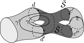
Figure 16. The curves $d,d^{\prime},c,c^{\prime},c^{\prime\prime},\gamma,\gamma^{\prime\prime}$ and the subsurfaces $\tilde{\mathcal{S}},\check{\mathcal{S}}$.

The four tori $c\times c^{\prime}$, $c\times c^{\prime\prime}$, $c\times d$ and $c\times d^{\prime}$ are contained in $C_{2}(\mathcal{S})$ and the equality

$$[c\times d]-[c\times d^{\prime}]+[c\times c^{\prime}]-[c\times c^{\prime\prime}]=0\in H_{2}(C_{2}(\mathcal{S}))$$

holds, as witnessed by the homology $c\times\check{\mathcal{S}}\subset C_{2}(\mathcal{S})$.

Moreover the classes $[c\times c^{\prime}]$ and $-[c\times c^{\prime\prime}]$ are equal: indeed there is an isotopy of $\mathcal{S}$ mapping $c$ to $c^{\prime}$ and $c^{\prime\prime}$ to $c$, as oriented curves; the class $[c\times c^{\prime\prime}]$ is mapped to the class $[c^{\prime}\times c]=-[c\times c^{\prime}]$.

Let again $[a]=[c\times c^{\prime}]$ and let $[b]=[c\times d]$: then the class $[b^{\prime}]=[c\times d^{\prime}]$ is equal to $[b]+2[a]\in H_{2}(C_{2}(\mathcal{S});\mathbb{Q})$.

Consider now an element of the Torelli group that fixes $c$ and maps $d$ to $d^{\prime}$ preserving the orientation, for example the bounding pair $D_{\gamma}\circ D_{\gamma^{\prime}}^{-1}$, where $\gamma$ and $\gamma^{\prime}$ are represented in Figure 16: then the class $b$ is mapped to $b^{\prime}=b+2a\neq b$. ∎

The previous proof works verbatim if we replace $\mathbb{Q}$ by any field of odd characteristic. Moreover all the arguments in the previous proof can be adapted to show that $H_{*}(F_{2}(\mathcal{S});\mathbb{F})$ is not a symplectic representation of $\Gamma_{g,1}$ (see Definition 2.1), where $\mathbb{F}$ is any field, including $\mathbb{Z}_{2}$.

Therefore, at least for orientable surfaces $\Sigma_{g,1}$ of genus $g\geq 2$, being a symplectic representation of the mapping class group seems to be a peculiarity of the homology of unordered configuration space and of the characteristic 2.

References

- [1] Joan S. L. Birman. Mapping class groups and their relationships to braid groups. Communications on Pure and Applied Math., 22:213–238, 1969.
- [2] Carl-Friedrich Bödigheimer, Frederick R. Cohen, and R. James Milgram. Truncated symmetric products and configuration spaces. Math. Zeitschrift, 214:179–216, 1993.
- [3] Carl-Friedrich Bödigheimer, Frederick R. Cohen, and Laurence R. Taylor. On the homology of configuration spaces. Topology, 28:111–123, 1989.
- [4] Carl-Friedrich Bödigheimer and Ulrike Tillmann. Stripping and splitting decorated mapping class groups. Progress in Mathematics, Birkäuser Verlag (Basel), 196, 2001.
- [5] Søren K. Boldsen. Improved homological stability for the mapping class group with integral or twisted coefficients. Mathematische Zeitschrift, 270:297–329, 2012.
- [6] Frederick R. Cohen, Thomas J. Lada, and J. Peter May. The homology of iterated loop spaces, volume 533 of Lecture Notes in Math. Springer Verlag, 1976.
- [7] Clifford J. Earle and Alfred Schatz. Teichmüller theory for surfaces with boundary. Journal of Diff. Geometry, 4:169–185, 1970.
- [8] Edward Fadell and Lee Neuwirth. Configuration spaces. Mathematica Scandinavica, 10:111–118, 1962.
- [9] Dmitry B. Fuchs. Cohomologies of the braid group mod 2. Functional Analysis and its Applications, 4:2:143–151, 1970.
- [10] Chad Giusti, Paolo Salvatore, and Dev Sinha. The mod-2 cohomology rings of symmetric groups. Journal of Topology, 5:169–198, 2012.
- [11] John Harer. Stability of the homology of the mapping class group of orientable surfaces. Annals of Mathematics, 121:215–249, 1985.
- [12] Ben Knudson. Betti numbers and stability for configuration spaces via factorization homology. Alg. and Geom. Topology, 17:3137–3187, 2017.
- [13] Peter Löffler and R. James Milgram. The structure of deleted symmetric products. Contemporary Math., 78:415–424, 1988.
- [14] Minoru Nakaoka. Homology of the infinite symmetric group. Annals of Mathematics, 73(2):229–257, 1961.
- [15] Oscar Randal-Williams. Resolutions of moduli spaces and homological stability. Journal of the European Mathematical Society, 18:1–81, 2016.