Computing the Scope of Applicability for Acquired Task Knowledge
in Experience-Based Planning Domains

Abstract

Experience-based planning domains have been proposed to improve problem solving by learning from experience. They rely on acquiring and using task knowledge, i.e., activity schemata, for generating solutions to problem instances in a class of tasks. Using Three-Valued Logic Analysis (TVLA), we extend previous work to generate a set of conditions that determine the scope of applicability of an activity schema. The inferred scope is a bounded representation of a set of problems of potentially unbounded size, in the form of a 3-valued logical structure, which is used to automatically find an applicable activity schema for solving task problems. We validate this work in two classical planning domains.

1 Introduction

Planning is a key ability for intelligent robots, increasing their autonomy and flexibility through the construction of sequences of actions to achieve their goals Ghallab et al. (2004). Planning is a hard problem and even what is known historically as classical planning is PSPACE-complete over propositional state variables Bylander (1994). To carry out increasingly complex tasks, robotic communities make strong efforts on developing robust and sophisticated high-level decision making models and implement them as planning systems. One of the most challenging issues is to find an optimum in a trade-off between computational efficiency and needed domain expert engineering work to build a reasoning system. In a recent work, Mokhtari et al. [2016b; 2016c; 2017b; 2017a] have proposed and integrated the notion of Experience-Based Planning Domain (EBPD)—a framework that integrates important concepts for long-term learning and planning—into robotics. An EBPD is an extension of the standard planning domains which in addition to planning operators, includes experiences and methods (called activity schemata) for solving classes of problems. The EBPDs framework consist of three components: experience extraction, conceptualization and planning. Experience extraction provides a human-robot interaction for teaching tasks and recording experiences of past robot’s observations and activities. Experiences are used to learn activity schemata, i.e., methods of guiding a search-based planner for finding solutions to other related problems. Conceptualization combines several techniques, including deductive generalization, different forms of abstraction, feature extraction and loop detection to generate activity schemata from experiences. Planning is a hierarchical problem solver which applies learned activity schemata for problem solving. In previous work, algorithms have been developed for experience extraction, activity schema learning and task planning [Mokhtari et al. 2016b; 2017b; 2017a].

As a contribution of this paper, we extend and improve the EBPDs framework to automatically retrieve an applicable activity schema for solving a task problem. We propose an approach to infer a set of conditions from an experience that determines the scope of applicability of an activity schema for solving a set of task problems. The inferred scope is a $3$-valued logical structure Kleene (1952) (i.e., a structure that extends Boolean logic by introducing an indefinite value $\frac{1}{2}$ to denote either $0$ or $1$) which associates a bounded representation for a set of $2$-valued logical structures of potentially unbounded size. We employ Three-Valued Logic Analysis (TVLA) Sagiv et al. (2002) both to infer the scope of applicability of activity schemata and to test whether existing activity schemata can be used to solve given task problems.

We recapitulate the prior work and present our approach to abstracting an experience and inferring the scope of applicability of an activity schema using the TVLA. We validate our system over two classical planning domains.

2 Related Work

The EBPDs’ objective is to perform tasks. Learning of Hierarchical Task Networks (HTNs) is among the most related works to EBPDs. In HTN planning, a plan is generated by decomposing a method for a given task into simpler tasks until primitive tasks are reached that can be directly achieved by planning operators. CaMeL Ilghami et al. (2002, 2005) is an HTN learner which receives as input plan traces and the structure of an HTN method and tries to identify under which conditions the HTN is applicable. CaMeL requires all information about methods except for the preconditions. The same group transcends this limitation in a later work Ilghami and Nau (2006) and presents the HDL algorithm which starts with no prior information about the methods but requires hierarchical plan traces produced by an expert problem-solver. HTN-Maker Hogg et al. (2008, 2016) generates an HTN domain model from a STRIPS domain model, a set of STRIPS plans, and a set of annotated tasks. HTN-Maker generates and traverses a list of states by applying the actions in a plan, and looks for an annotated task whose effects and preconditions match some states. Then it regresses the effects of the annotated task through a previously learned method or a new primitive task. Overall, identifying the hierarchical structure is an issue, and most of the techniques in HTN learning rely on the hierarchical structure of the HTN methods specified by a human expert. By contrast, the EBPDs framework presents a fully autonomous approach to learning activity schemata with loops (an alternative to recursive HTN methods) from single experiences.

Aranda Srivastava et al. (2011) takes a planning problem and finds a plan that includes loops. Using TVLA Lev-Ami and Sagiv (2000) and back-propagation, Aranda finds an abstract state space from a set of concrete states of problem instances with varying numbers of objects that guarantees completeness, i.e., the plan works for all inputs that map onto the abstract state. These strong guarantees come at a cost: (i) restrictions on the language of actions; and (ii) high running times. Indeed computing the abstract state is worst-case doubly-exponential in the number of predicates. In contrast, the EBPDs system assumes standard PDDL actions. We also use TVLA to compute an abstract structure that determines the scope of applicability of an activity schema, however, we trade completeness for a polynomial time algorithm, which results in dramatically better performance.

LoopDistill Winner and Veloso (2007) also learns plans with loops from example plans. It identifies the largest matching sub-plan in a given example and converts the repeating occurrences of the sub-plans into a loop. The result is a domain-specific planning program (dsPlanner), i.e., a plan with if-statements and while-loops that can solve similar problems of the same class. LoopDistill, nonetheless, does not address the applicability test of plans.

Other approaches in AI planning including case based planning Hammond (1986); Borrajo et al. (2015), and macro operators Fikes et al. (1972); Chrpa (2010) can also be related to our work. These methods tend to suffer from the utility problem, in which learning more information can be counterproductive due to the difficulty with storage and management of the information and with determining which information should be used to solve a particular problem. In EBPDs, by combining generalization with abstraction in task learning, it is possible to avoid saving large sets of concrete cases. Additionally, since in EBPDs, task learning is supervised, solving the utility problem can be to some extent delegated to the user, who chooses which tasks and associated procedures to teach.

3 The Prior Work

An EBPD $\mathcal{D=\langle A,O,E,M\rangle}$ relies on a set of abstract planning operators $\mathcal{A}$, a set of concrete planning operators $\mathcal{O}$, a set of experiences $\mathcal{E}$, and a set of activity schemata (i.e., task planning models) $\mathcal{M}$, for problem solving.

Any planning operator $o\in(\mathscr{A\lor O})$ is a tuple $\langle h,S,P,E\rangle$, where $h$ is the operator head, $S$ is a set of atoms describing the static part of the world information, $P$ is the precondition (a conjunction of atoms that must be available in a state in order to apply $o$), and $E$ is the effect (a set of atoms that specifies the changes on a state effected by $o$). The abstract and concrete planning operators are linked together using an operator abstraction hierarchy (specified by a parent property in concrete planning operators), for example, (pick ?block ?table) is an abstract operator for the concrete operator (pick ?hoist ?block ?table ?location). More in Mokhtari et al. (2017b).

An experience $e\in\mathcal{E}$ is a triple of ground structures $\langle t,K,\pi\rangle$, where $t$ is the task achieved in an experience, e.g., (stack t1 t2), $K$ is a set of key-properties, i.e., a set of predicates with temporal symbols, to describe the experience, and $\pi$ is a plan to achieve $t$. The temporal symbols for representing key-properties are: static—always true during an experience, init—true at the initial state, and end—true at the final state. Listing 1 shows part of an experience . This experience is used to illustrate the proposed approach in this paper.

⬇

(:task stack

:parameters (t1 t2)

:key-properties ((static(table t1))

(static(pile t2))

(static(location l1))

(static(hoist h1))

(static(attached t2 l1))

(static(attached t1 l1))

(static(belong h1 l1))

(static(pallet p1))

(static(block b1))

(static(block b2))

$\cdots$

(static(block b7))

(static(block b8))

(static(blue b1))

(static(blue b2))

$\cdots$

(static(red b7))

(static(red b8))

(init(top p1 t2))

(init(ontable b1 t1))

(init(ontable b2 t1))

$\cdots$

(init(ontable b7 t1))

(init(ontable b8 t1))

(init(at h1 t1))

(init(empty h1))

(end(on b1 p1))

(end(on b2 b1))

$\cdots$

(end(on b7 b6))

(end(on b8 b7))

(end(top b8 t2)))

:plan ((pick h1 b1 t1 l1)

(move h1 t1 t2 l1)

(stack h1 b1 p1 t2 l1)

(move h1 t2 t1 l1)

(pick h1 b2 t1 l1)

(move h1 t1 t2 l1)

(stack h1 b2 b1 t2 l1)

$\cdots$

(pick h1 b8 t1 l1)

(move h1 t1 t2 l1)

(stack h1 b8 b7 t2 l1)))

Listing 1: Part of the ‘stack’ experience in the stack domain. There are 8 (4 blue and 4 red) blocks in this experience. The goal of the task in this experience is to stack the blocks (that are initially on a table) on a pile with blue blocks at the bottom and red blocks on the top. The key-properties describe the initial, final and static world information of the experience. The solution plan contains 31 actions.

An activity schema $m\in\mathcal{M}$ is a pair of ungrounded structures $\langle h,\Omega\rangle$, where $h$ is the target task, e.g., (stack ?t1 ?t2), and $\Omega$ is an abstract plan to achieve the task in $m$, i.e., a sequence or loops of abstract operators. Each abstract operator in the abstract plan is in the form $(a,F)$ where $a$ is an abstract operator head, and $F$ is a set of features, i.e., key-properties in an experience that describe the arguments of $a$. A concrete example of an activity schema is given in the rest of the paper.

3.1 Acquiring Activity Schemata in EBPDs

Activity schemata are acquired from single experiences through a conceptualization methodology:

Following the tradition of PLANEX Fikes et al. (1972) and Explanation-Based Generalization [Mitchell et al., 1986], all constants appearing in the actions as well as in the key-properties of an experience are variablized. The obtained generalized experience forms the basis of the activity schema.

After the generalization, concrete actions in the plan of the generalized experience are replaced with abstract actions, as specified in the operator abstraction hierarchy. That is, some concrete actions are excluded from the abstract plan, and some arguments of the concrete actions are excluded from the arguments of the respective abstract actions.

Then, all potential key-properties (i.e., features) that link the arguments of the abstract actions with the parameters of the experience are extracted and associated to the abstract actions. For example in Listing 1, the key-property (init(ontable b1 t1)) is a feature that links b1, an argument of an (abstract) action pick, to t1, a parameter of the task stack. During problem solving features determine which objects in a given problem are preferable to instantiate abstract actions.

Finally, potential loops of actions in the activity schema are detected. Mokhtari et al. Mokhtari et al. (2017b) propose a Contiguous Non-overlapping Longest Common Prefix (CNLCP) algorithm. CNLCP is an extension of the standard function of constructing the Longest-Common-Prefix (LCP) array—an array storing the lengths of the longest common-prefixes of consecutive suffixes in a suffix array Manber and Myers (1993). CNLCP first computes a Non-overlapping LCP (NLCP) array between all consecutive suffixes (in a suffix array) such that the lengths of the longest common prefixes between every two suffixes must be at most equal to the difference in lengths between the two suffixes, and then preserves only consecutive NLCPs. When a loop is detected, the respective loop iterations are merged together. Listing 2 shows part of the learned activity schema for the ‘stack’ experience in Listing 1.

3.2 Task Planning in EBPDs

Task planning in EBPDs is achieved by a hierarchical planning system, called Schema-Based Planner (SBP), consisting of an abstract and a concrete planner Mokhtari et al. (2017b). A task planning problem is a tuple $\mathcal{P}=\langle t,\sigma,s_{0},g\rangle$ where $t$ is the target task, e.g., (stack t1 t2), $\sigma$ is static world information, $s_{0}$ is the initial state, and $g$ is the goal.

Given the abstract and concrete planning operators $(\mathscr{A,O})$, and an activity schema $m$, SBP applies $m$ to generate a plan for $\mathscr{P}$. The abstract planner first drives an abstract solution to $\mathscr{P}$ by generating instances of the abstract actions (of the abstract plan) in $m$. It also extends possible loops in $m$ for the applicable objects in $\mathscr{P}$. To extend a loop, the abstract planner simultaneously generates all successors for an iteration of the loop as well as for the following abstract action after the loop. It then computes a cost for all generated successors based on the number of features of abstract actions (in $m$) verified with the features extracted for the instantiated abstract actions, and selects the best current action with the lowest cost during the search. Finally, the abstract planner generates a ground abstract plan when it gets the end of (the abstract plan of) $m$.

The produced ground abstract plan becomes the main skeleton of the final solution based on which the concrete planner generates a final plan by instantiating and substituting concrete actions for the abstract actions (as specified in the operator abstraction hierarchy).

See [Mokhtari et al. 2017a; 2017b] for the algorithms of learning activity schemata and task planning in EBPDs.

⬇

(:method stack

:parameters (?t1 ?t2)

:abstract-plan

((!pick ?b1 ?t1)

((static(blue ?b1))$\cdots$)

(!stack ?b1 ?p1 ?t2)

((static(blue ?b1))(static(pallet ?p1))$\cdots$)

(loop (!pick ?b2 ?t1)

((static(blue ?b2))$\cdots$)

(!stack ?b2 ?b1 ?t2)

((static(blue ?b1))(static(blue ?b2))$\cdots$))

(!pick ?b5 ?t1)

((static(red ?b5))$\cdots$)

(!stack ?b5 ?b4 ?t2)

((static(blue ?b4))(static(red ?b5))$\cdots$)

(loop (!pick ?b6 ?t1)

((static(red ?b6))$\cdots$)

(!stack ?b6 ?b5 ?t2)

((static(red ?b5))(static(red ?b6))$\cdots$))

(!pick ?b8 ?t1)

((static(red ?b8))(end(top ?b8 ?t2))$\cdots$)

(!stack ?b8 ?b7 ?t2)

((static(red ?b7))(static(red ?b8))$\cdots$)))

Listing 2: Part of a learned activity schema for the ‘stack’ task with two loops. From Listing 1, the constants are replaced with variables (Generalization), some actions are excluded from the abstract plan (Operator abstraction), abstract actions are associated with features (Feature extraction), and repetitive abstract actions with same features form loops (Loop detection). See Mokhtari et al. (2017b).

4 Inferring the Scope of Applicability

In the previous work, the EBPDs framework lacked a strategy to find an applicable activity schema, among several learned activity schemata, for solving a task problem. We extend the EBPDs framework to infer the scope of an activity schema from the key-properties of an experience in the form of a $3$-valued logical structure. This allows for the applicability test of an activity schema to solve a set of task problems. We employ Canonical Abstraction Sagiv et al. (2002) which associates a bounded representation for any (possibly infinite) set of logical structures of potentially unbounded size.

To infer the scope of an activity schema, we first represent (the key-properties of) an experience in a $2$-valued structure:

Definition 1.

A $2$-valued logical structure, also called a concrete structure, over a finite set of predicates $\mathscr{V}$ is a pair, $S=\langle U,\iota\rangle$, where $U$ is the universe of the $2$-valued structure and $\iota$ is the interpretation function that maps predicates to their truth-values in the structure: for every predicate $p^{k}\in\mathscr{V}$ of arity $k$, $\iota(p):U^{k}\to\{0,1\}$.

We convert a set of key-properties $K$ to the $2$-valued structure $\textit{Struc}(K)=(U,\iota)$ as follows:

$$\small\begin{array}[]{rcl}U&=&\bigcup\limits_{\tau(p(t_{1},\ldots,t_{k}))\in K}\{t_{1},\ldots,t_{k}\}\\ \mathscr{V}&=&\bigcup\limits_{\tau(p(t_{1},\ldots,t_{k}))\in K}\big{\{}\tau(p)~{}|~{}\tau\in\{\small\text{static},\text{init},\text{end}\}\big{\}}\\ \iota&=&\lambda\tau(p^{k})\in\mathscr{V}.\\ &&\lambda(t_{1},\ldots,t_{k})\in{U}^{k}.\ \left\{\begin{array}[]{ll}1,&\hbox{if}\enspace\tau(p(t_{1},\ldots,t_{k}))\in K\hbox{;}\\ 0,&\hbox{otherwise.}\end{array}\right.\end{array}$$

That is, the universe of $\textit{Struc}(K)$ consists of the objects appearing in the key-properties of $K$, and the interpretation is defined over the key-properties of $K$. The interpretation of a key-property $\tau(p)$, where $\tau\in\{\text{static},\text{init},\text{end}\}$, is $1$ if the corresponding key-property appears in $K$; and $0$ otherwise.

Fig. 1(a) shows a $2$-valued structure $C$ representing the (generalized) experience in Listing 1. In this example, the universe, the set of predicates and truth-values (interpretations) of the predicates over the universe of $C$ are as follows:

$$U =\{\text{?t1,?t2,?l1,?h1,?p1,?b1,?b2,?b3,}\dots\}$$

$$\mathscr{V} =\{\text{(static(block)),(init(ontable)),(end(on)),}\dots\}$$

$$\iota =\{\text{(static(table ?t1)),(static(block ?b1)),}\dots\}\enspace.$$

The scope inference (i.e., abstraction) is based on Kleene’s $3$-valued logic Kleene (1952), which extends Boolean logic by introducing an indefinite value $\frac{1}{2}$, to denote either $0$ or $1$.

Definition 2.

A $3$-valued logical structure, also called an abstract structure, over a finite set of predicates $\mathscr{V}$ is a pair $S=\langle U,\iota\rangle$ where $U$ is the universe of the $3$-valued structure and $\iota$ is the interpretation function mapping predicates to their truth-values in the structure: for every predicate $p\in\mathscr{V}$ of arity $k$, $\iota(p):U^{k}\to\{0,1,\frac{1}{2}\}$.

A $3$-valued structure may include summary objects, i.e., objects that correspond to one or more objects in a $2$-valued structure represented by the $3$-valued structure.

Fig. 1(b) shows a $3$-valued structure $S$ of the $2$-valued structure $C$ in Fig. 1(a). Double circles stand for summary objects and solid (dashed) arrows represent truth-values of $1$ ($\frac{1}{2}$). Intuitively, because of the summary objects, the $3$-valued structure $S$ represents the $2$-valued structure $C$ and all other ‘stack’ problems that have exactly one table, one pile, one location, one hoist, one pallet, and at least one blue block and one red block such that the blocks are initially on a table and finally red blocks are on top of blue blocks in a pile.

The objects in a $2$-valued structure are merged into a summary object in a $3$-valued structure as follows:

Definition 3.

Let $\mathscr{V}^{(k)}$ denotes a set of predicates of arity $k$, and $C=\langle U,\iota\rangle$ is a $2$-valued structure. The canonical name of an object $u\in U$, also called an abstraction predicate, denoted by ${\text{canon}}(u)$, is a set of unary predicates that hold for $u$ in $C$: ${\text{canon}}(u)=\{p\in\mathscr{V}^{(1)}\mid\iota(p)(u)=1\}.$

For example, the canonical names of the objects in structure $C$ of Fig. 1(a) are the following:

$$\small\begin{array}[]{rcl}{\text{canon}}(\text{?t1})&=&\{\text{static(table)}\}\\ {\text{canon}}(\text{?t2})&=&\{\text{static(pile)}\}\\ {\text{canon}}(\text{?l1})&=&\{\text{static(location)}\}\\ {\text{canon}}(\text{?h1})&=&\{\text{static(hoist),init(empty)}\}\\ {\text{canon}}(\text{?p1})&=&\{\text{static(pallet)}\}\\ {\text{canon}}(\text{?b1..?b4})&=&\{\text{static(block),static(blue)}\}\\ {\text{canon}}(\text{?b5..?b8})&=&\{\text{static(block),static(red)}\}\enspace.\end{array}$$

Definition 4.

Let $\mathscr{V}$ be a set of predicates, $C=\langle U,\iota\rangle$ a $2$-valued structure, and $S=\langle U^{\prime},\iota^{\prime}\rangle$ a $3$-valued structure, over $\mathscr{V}$. A summary object $w\in U^{\prime}$ corresponds to two objects $(u,v)\in U$, if ${\text{canon}}(u)={\text{canon}}(v)$.

For example, the objects (?b1..?b4) in Fig. 1(a) with the same canonical name are merged into a summary object.

Each $2$-valued structure $C$ is represented by its canonical abstraction, i.e., a $3$-valued structure in which all objects in $C$ with the same canonical name are merged into a summary element of that canonical name:

Definition 5.

Let $\mathscr{V}$ be a set of predicates, and $C=\langle U,\iota\rangle$ a $2$-valued structure. The Canonical abstraction of $C$, denoted by $\beta(C)$, is a $3$-valued structure $S=\langle U^{\prime},\iota^{\prime}\rangle$ as follow:

$$U^{\prime}=\{{\text{canon}}(u)\mid u\in U\}$$

$$\iota^{\prime}(p)(t_{1}^{\prime},\ldots,t_{k}^{\prime})=$$

$$\bigsqcup\limits_{t_{1},\ldots,t_{k}}\{\iota(p)(t_{1},\ldots,t_{k})\mid\forall i=1..k.\ t_{i}^{\prime}={\text{canon}}(t_{i})\}\enspace.$$

The canonical abstraction is based on Kleene’s join operation $\sqcup:2^{\{0,1,\frac{1}{2}\}}\rightarrow\{0,1,\frac{1}{2}\}$, which overapproximates non-empty sets of logical values as follows:

$$\sqcup\mathscr{V}=\left\{\begin{array}[]{ll}v,&\hbox{if}\enspace\mathscr{V}=\{v\}\hbox{;}\\ \frac{1}{2},&\hbox{otherwise.}\end{array}\right.$$

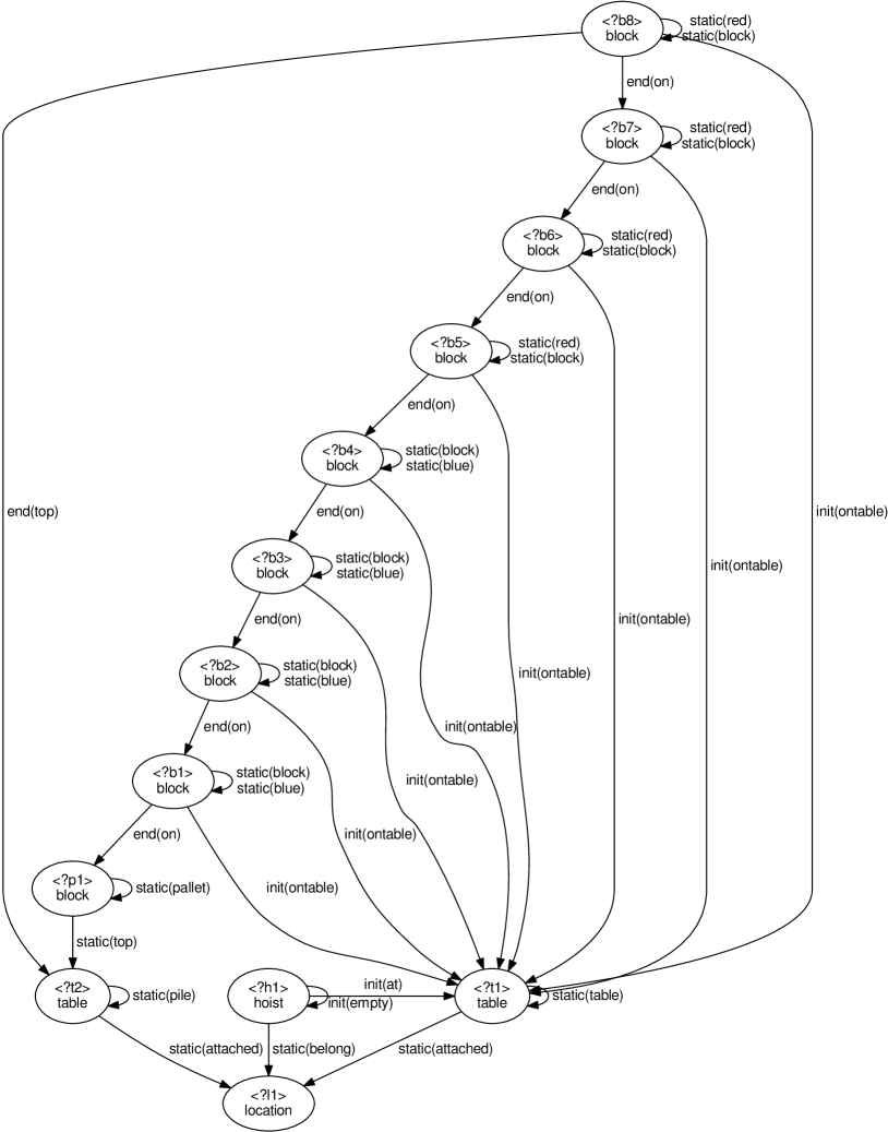
(a) A $2$-valued structure $C$.

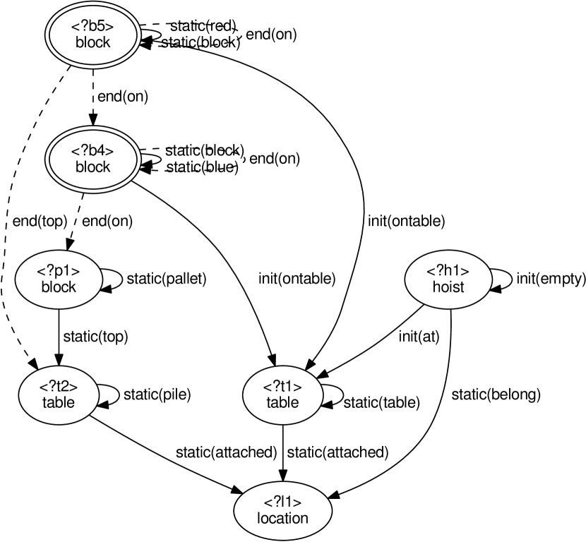
(b) A $3$-valued structure $S=\beta(C)$.

Figure 1: Canonical abstraction of the (generalized) ‘stack’ experience (see Listing 1). Nodes constitute the universe of a structure and edges represent the truth-values of the key-properties. The nodes ?b4 and ?b5 are summary objects that represent all blocks of the same properties (i.e., blue/red) in an experience (or in a problem).

Kleene’s join operation determines the truth-value (interpretation) of key-properties in a $3$-valued structure. The interpretation of a key-property in the $3$-valued structure is $1$ (solid arrows) if that key-property exists for all objects of the same canonical name in the $2$-valued structure; the truth-value is $\frac{1}{2}$ if the key-property exists for some objects of the same canonical name (dashed arrows); and $0$ otherwise.

The inferred scope is finally represented as a set of key-properties. A summary object ?o is represented by a proposition of the form (summary ?o). An indefinite (i.e., $\frac{1}{2}$-valued) key-property $p$ appears as (maybe $p$). Listing 3 shows the inferred scope for the ‘stack’ activity schema.

⬇

(:method stack

:parameters (?table ?pile)

:scope ((summary ?b4)

(summary ?b5)

(static(red ?b5))

(static(attached ?t2 ?l1))

(static(attached ?t1 ?l1))

(static(block ?b4))

(static(block ?b5))

(static(belong ?h1 ?l1))

(static(pallet ?p1))

(static(blue ?b4))

(static(pile ?t2))

(static(top ?p1 ?t2))

(static(table ?t1))

(init(ontable ?b4 ?t1))

(init(ontable ?b5 ?t1))

(init(at ?h1 ?t1))

(init(empty ?h1))

(maybe(end(top ?b5 ?t2)))

(maybe(end(on ?b5 ?b5)))

(maybe(end(on ?b4 ?p1)))

(maybe(end(on ?b5 ?b4)))

(maybe(end(on ?b4 ?b4))))

:abstract-plan (the same as in Listing 2))

Listing 3: The scope of the activity schema for the ‘stack’ task.

5 Testing the Scope of Applicability

An activity schema is applicable for solving a task problem if the task problem is embedded in the scope of the activity schema (i.e., the task problem maps onto the scope of the activity schema). For this purpose, we convert a task problem $\mathscr{P}=\langle t,\sigma,s_{0},g\rangle$ into a $2$-valued structure (as described in the previous section), and then test if the obtained $2$-valued structure is embedded in the scope of an activity schema:

Definition 6.

We say that a $2$-valued structure (i.e., a task problem represented in a $2$-valued structure) $C=\langle U,\iota\rangle$ is embedded in a $3$-valued structure (i.e., the scope of an activity schema) $S=\langle U^{\prime},\iota^{\prime}\rangle$, denoted by $C\sqsubseteq S$, if there exists a function $f:U\to U^{\prime}$ such that $f$ is surjective and for every predicate $p$ of arity $k$ and tuple of objects $u_{1},...,u_{k}\in U$, one of the following conditions holds:

$$\begin{array}[]{c}\iota(p)(u_{1},...,u_{k})=\iota^{\prime}(p)(f(u_{1}),...,f(u_{k}))\quad\text{or}\\ \iota^{\prime}(p)(f(u_{1}),...,f(u_{k}))=\frac{1}{2}\enspace.\end{array}$$ (1)

Further, a $3$-valued structure $S$ represents the set of $2$-valued structures embedded in it: $\{C\mid C\sqsubseteq S\}$.

Proposition 1.

Canonical abstraction is sound with respect to the embedding relation. That is, $C\sqsubseteq\beta(C)$ holds for every $2$-valued structure $C$.

We implemented and integrated an Embedding function into the EBPDs’ planning system which finds an applicable activity schema $m$ with the scope of applicability $S$ to a task problem $\mathscr{P}$, by checking whether $\textit{Struc}(\mathscr{P})\sqsubseteq S$ holds.

6 Experimental Resutls

We implemented a prototype of this system in Prolog and used TVLA Lev-Ami et al. (2004) as an engine, implemented in Java, for computing the scope of applicability of activity schemata. We develop two EBPDs based on classical planning domains and evaluate our system in classes of tasks in these domains.

STACK. In the first experiment, we develop the stack domain, based on the blocks world domain, containing the concrete planning operators, move/4, pick/4, put/4, stack/5, unstack/5, and the abstract planning operators, pick/3, put/3, stack/4, unstack/4 (i.e., the numbers indicate arities). The main objective of this experiment is to learn different activity schemata (tasks) with the same goal but different scopes of applicability, and to evaluate how the scope testing (embedding) function allows the system to automatically find an applicable activity schema to a given task problem.

In the paper, we described a class of ‘stack’ problems with an experience (in Listing 1), a learned activity schema (in Listing 2), and its scope of applicability (in Listing 3 and Fig. 1(b)). Additionally, we define three other classes of the ‘stack’ problems with the same goal but different initial configurations as follows: (i) a pile of red and blue blocks, with red blocks at the bottom and blue blocks on the top; (ii) a pile of alternating red and blue blocks, with a blue block at the bottom and a red block on the top; and (iii) a pile of alternating red and blue blocks, with a red block at the bottom and a blue block on the top. In all classes of problems, the goal is to make a new pile of red and blue blocks with blue blocks at the bottom and red blocks on the top.

To show the effectiveness of the proposed scope inference, we simulated an experience (containing an equal number of $20$ blocks of red and blue colors) in each of the above classes. Based on these experiences the system generates three activity schemata with distinct scopes of applicability (see Fig. 2).

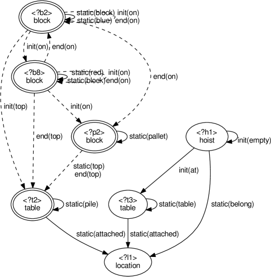
(a) This scope of applicability (abstract structure) represents all ‘stack’ problems that have exactly one table and at least one pile, one pallet, one blue block and one red block such that blue blocks are initially on top of red blocks and finally red blocks are on top of blue blocks (on a pallet) on a pile.

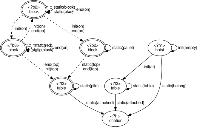
(b) This scope of applicability represents all ‘stack’ problems that have exactly one table and at least one pile, one pallet, one blue block and one red block such that alternate red and blue blocks are initially on a pile with a blue block at the bottom (on a pallet) and a red block on top and finally red blocks are on top of blue blocks.

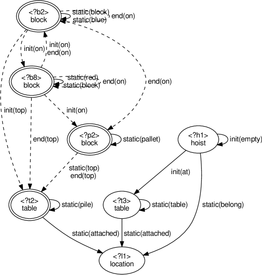
(c) This scope of applicability represents all ‘stack’ problems that have exactly one table and at least one pile, one pallet, one blue block and one red block such that alternate red and blue blocks are initially on a pile with a red block at the bottom (on a pallet) and a blue block on top and finally red blocks are on top of blue blocks.

Figure 2: The scope of applicability, i.e., canonical abstraction, of the additional three classes of the ‘stack’ task in the stack domain.

To evaluate the system over the learned activity schemata, we randomly generated $60$ task problems in all four classes of the ‘stack’ tasks, ranging from $20$ to $50$ equal number of red and blue blocks in each problem. In this experiment, the system found applicable activity schemata to solve given task problems in under $60\text{ms}$ for testing the scope of applicability (see Fig. 3) and then successfully solved all problems. To show the efficiency of the system, we also evaluated and compared the performance of the SBP with a state-of-the-art planner, Madagascar Rintanen (2012), based on four measures: time, memory, number of evaluated nodes and plan length (see Fig. 4). In this experiment, SBP was extremely efficient in terms of memory and evaluated nodes in the search tree. Note that the time comparison is not accurate, since SBP has been implemented in Prolog, in contrast to Madagascar that has been implemented in C++.

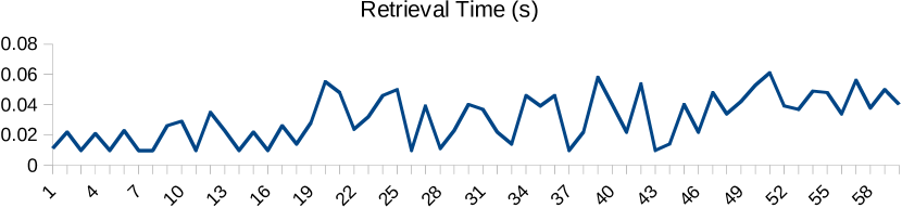
Figure 3: CPU time used by SBP to find an applicable activity schema (among 4) for solving problems in the stack domain.

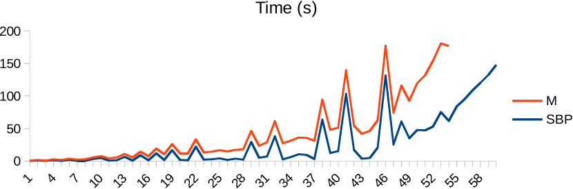
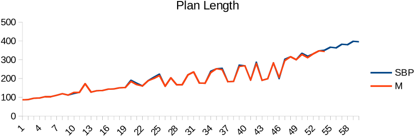
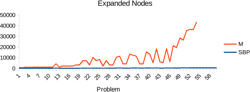
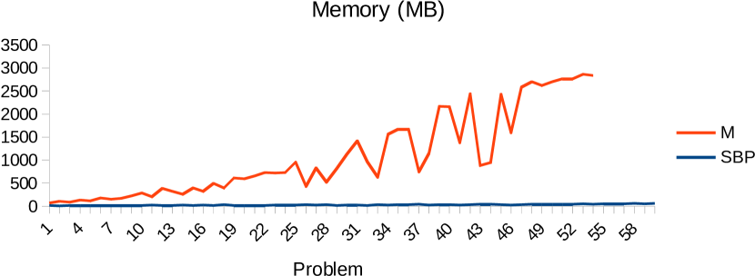
Figure 4: Performance of the SBP and Madagascar (M) in the stack domain.

ROVER. In the second experiment, we used the rover domain from the 3rd International Planning Competition (IPC-3). In this experiment, we adopt a different approach for evaluating the proposed scope inference technique. We randomly generated $50$ problems containing exactly $1$ rover and ranging from $1$ to $3$ waypoints, $5$ to $30$ objectives, $5$ to $10$ cameras and $5$ to $20$ goals in each problem. Using the scope inference procedure, the problems are classified into $9$ sets of problems. That is, problems that converge to the same $3$-valued structure are put together in the same set. Hence, each set of problems is identified with a distinct scope of applicability. Fig. 5(a) shows the time required to classify the problems into different sets, i.e., the time required by TVLA to generate $3$-valued structures for the problems and test which problems converge to the same $3$-valued structure. Fig. 5(b) shows the distribution of the problems in the obtained sets of problems. In each set of problems, we simulated an experience and generated an activity schema for problem solving. Fig. 6 shows the time required to retrieve an applicable activity schema (among 9 activity schemata in this experiment) for solving given problems, i.e., the time required to check whether a given problem is embedded in the scope of an activity schema. SBP successfully solved all problems in each class.

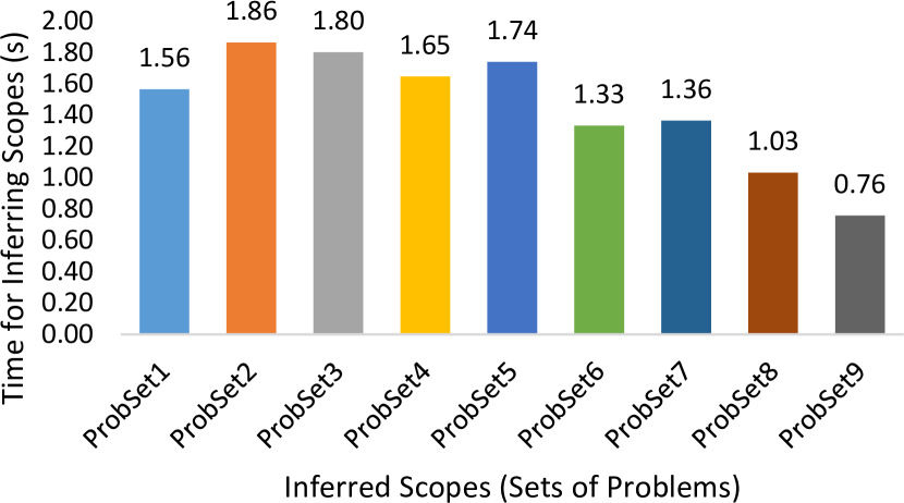
(a)

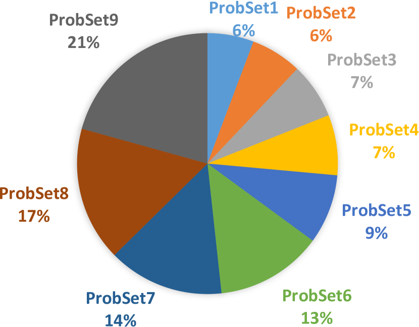
(b)

Figure 5: CPU time used by TVLA to classify the problems (a), and distribution of the problems in the obtained problem sets (b) in the rover domain

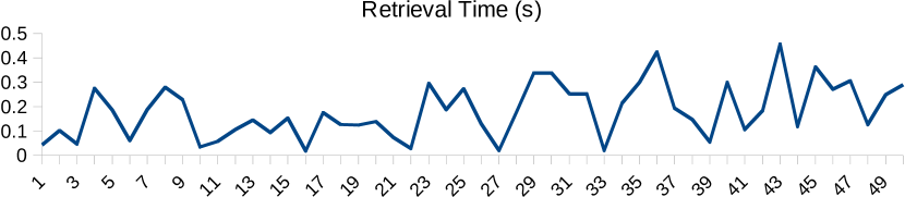
Figure 6: CPU time used by SBP to find an applicable activity schema (among 9) for solving problems in the rover domain.

7 Conclusion and Future Work

Using TVLA we generated a set of conditions that determine the scope of applicability of an activity schema in experience-based planning domains (EBPDs). The inferred scope allows an EBPD system to automatically find an applicable activity schema for solving a task problem. We validated this work in two classical planning domains. The initial results show good scalability, however, engineering optimizations are possible on the prototype implementation of the proposed algorithms. This work is extensively presented in Mokhtari et al. (2019).

References

- Borrajo et al. [2015] Daniel Borrajo, Anna Roubíčková, and Ivan Serina. Progress in case-based planning. ACM Computing Surveys (CSUR), 47(2):35:1–35:39, Jan 2015.
- Bylander [1994] Tom Bylander. The computational complexity of propositional STRIPS planning. Artificial Intelligence, 69(1-2):165–204, 1994.
- Chrpa [2010] Lukáš Chrpa. Generation of macro-operators via investigation of action dependencies in plans. The Knowledge Engineering Review, 25(03):281–297, 2010.
- Fikes et al. [1972] Richard E Fikes, Peter E. Hart, and Nils J Nilsson. Learning and executing generalized robot plans. Artificial intelligence, 3:251–288, 1972.
- Ghallab et al. [2004] Malik Ghallab, Dana Nau, and Paolo Traverso. Automated planning: theory & practice. Elsevier, 2004.
- Hammond [1986] Kristian J Hammond. CHEF: a model of case-based planning. In Proceedings of the Fifth National Conference on Artificial Intelligence, pages 267–271. AAAI Press, 1986.
- Hogg et al. [2008] Chad Hogg, Héctor Munoz-Avila, and Ugur Kuter. HTN-MAKER: learning HTNs with minimal additional knowledge engineering required. In Proceedings of the Twenty-Third AAAI Conference on Artificial Intelligence, pages 950–956. AAAI Press, 2008.
- Hogg et al. [2016] Chad Hogg, Héctor Muñoz-Avila, and Ugur Kuter. Learning hierarchical task models from input traces. Computational Intelligence, 32(1):3–48, 2016.
- Ilghami and Nau [2006] Okhtay Ilghami and Dana S Nau. Learning to do HTN planning. In 16st International Conference on Automated Planning and Scheduling (ICAPS), pages 390–393. AAAI Press, 2006.
- Ilghami et al. [2002] Okhtay Ilghami, Dana S Nau, Héctor Munoz-Avila, and David W Aha. CaMeL: learning method preconditions for HTN planning. In Proceedings of the Sixth International Conference on Artificial Intelligence Planning Systems (AIPS), pages 131–142, 2002.
- Ilghami et al. [2005] Okhtay Ilghami, Dana S Nau, Héctor Munoz-Avila, and David W Aha. Learning preconditions for planning from plan traces and HTN structure. Computational Intelligence, 21(4):388–413, 2005.
- Kleene [1952] Stephen Cole Kleene. Introduction to metamathematics, volume 483. D. Van Nostrand Co., Inc., New York, N. Y., 1952.
- Lev-Ami and Sagiv [2000] Tal Lev-Ami and Shmuel Sagiv. TVLA: A system for implementing static analyses. In Static Analysis, 7th International Symposium, SAS 2000, Santa Barbara, CA, USA, June 29 - July 1, 2000, Proceedings, pages 280–301, 2000.
- Lev-Ami et al. [2004] Tal Lev-Ami, Roman Manevich, and Mooly Sagiv. TVLA: a system for generating abstract interpreters. In Building the Information Society, pages 367–375. Springer, 2004.
- Manber and Myers [1993] Udi Manber and Gene Myers. Suffix arrays: a new method for on-line string searches. SIAM Journal on Computing, 22(5):935–948, 1993.
- Mitchell et al. [1986] Tom M. Mitchell, Richard M. Keller, and Smadar T. Kedar-Cabelli. Explanation-based generalization: a unifying view. Machine Learning, 1(1):47–80, 1986.
- Mokhtari et al. [2016a] Vahid Mokhtari, GiHyun Lim, Luís Seabra Lopes, and Armando J. Pinho. Gathering and conceptualizing plan-based robot activity experiences. In Emanuele Menegatti, Nathan Michael, Karsten Berns, and Hiroaki Yamaguchi, editors, Intelligent Autonomous Systems 13, volume 302 of Advances in Intelligent Systems and Computing, pages 993–1005. Springer International Publishing, 2016.
- Mokhtari et al. [2016b] Vahid Mokhtari, Luís Seabra Lopes, and Armando J. Pinho. Experience-based planning domains: an integrated learning and deliberation approach for intelligent robots. Journal of Intelligent & Robotic Systems, 83(3):463–483, 2016.
- Mokhtari et al. [2016c] Vahid Mokhtari, Luís Seabra Lopes, and Armando J. Pinho. Experience-based robot task learning and planning with goal inference. In 26st International Conference on Automated Planning and Scheduling (ICAPS), pages 509–517. AAAI Press, June 2016.
- Mokhtari et al. [2017a] Vahid Mokhtari, Luís Seabra Lopes, and Armando J. Pinho. An approach to robot task learning and planning with loops. In 2017 IEEE/RSJ International Conference on Intelligent Robots and Systems (IROS), pages 6033–6038, September 2017.
- Mokhtari et al. [2017b] Vahid Mokhtari, Luís Seabra Lopes, and Armando J. Pinho. Learning robot tasks with loops from experiences to enhance robot adaptability. Pattern Recognition Letters, 99(Supplement C):57 – 66, 2017. User Profiling and Behavior Adaptation for Human-Robot Interaction.
- Mokhtari et al. [2019] Vahid Mokhtari, Luís Seabra Lopes, Armando Pinho, and Roman Manevich. Learning task knowledge and its scope of applicability in experience-based planning domains. arXiv preprint arXiv:1902.10770, 2019.
- Rintanen [2012] Jussi Rintanen. Planning as satisfiability: heuristics. Artificial Intelligence, 193:45 – 86, 2012.
- Sagiv et al. [2002] Shmuel Sagiv, Thomas W. Reps, and Reinhard Wilhelm. Parametric shape analysis via 3-valued logic. ACM Trans. Program. Lang. Syst., 24(3):217–298, 2002.
- Srivastava et al. [2011] Siddharth Srivastava, Neil Immerman, and Shlomo Zilberstein. A new representation and associated algorithms for generalized planning. Artificial Intelligence, 175(2):615 – 647, 2011.
- Winner and Veloso [2007] Elly Winner and Manuela M. Veloso. LoopDISTILL: learning domain-specific planners from example plans. In Workshop on AI Planning and Learning, ICAPS, 2007.