An Exact Algorithm for Minimum Weight Vertex Cover Problem in Large Graphs

Abstract

This paper proposes a novel branch-and-bound (BMWVC) algorithm to exactly solve the minimum weight vertex cover problem (MWVC) in large graphs. The original contribution is several new graph reduction rules, allowing to reduce a graph $G$ and the time needed to find a minimum weight vertex cover in $G$. Experiments on large graphs from real-world applications show that the reduction rules are effective and the resulting BMWVC algorithm outperforms relevant exact and heuristic MWVC algorithms.

Introduction

Nowadays, very large graphs are often used in information technology to model things such as computer networks, social networks, mobile call networks, and biological networks. These graphs usually share common characteristics: very low density, a huge number of vertices, and the vertex degrees following some statistical property Newman (2003). Recently, algorithms in large sparse graphs have become an extensively studied topic with a large number of applications. Vertex cover problem is one of the earliest and most common graph problems. A vertex cover of an undirected graph $G=(V,E)$, where $V$ is a set of vertices and $E$ is a set of edges, is a subset of vertices $S\subseteq V$ such that every edge of $E$ has at least one of its endpoint vertices in $S$. The minimum vertex cover problem (MVC) of $G$ is to find a vertex cover with the smallest number of vertices. An important generalized version of MVC is the minimum weight vertex cover problem (MWVC), in which a weight is associated with each vertex of $G$, and the problem is to find a vertex cover of minimum total weight in $G$.

MWVC is NP-hard Garey (1979), and is closely related to the well-known maximum weight independent set problem (MWIS) and the maximum weight clique problem (MWC). MWVC, MWIS and MWC are three important vertex-weighted graph problems that play a vital role in numerous real-world applications such as wireless communication Wang et al. (2015, 2017), network flows Benlic and Hao (2013), protein structure prediction Mascia et al. (2010), coding theory Zhian et al. (2013), and computer vision Ma and Jan Latecki (2013).

A remarkable number of local search algorithms for MWVC have been proposed in the literature, including the ant colony optimization algorithms Shyu et al. (2004); Jovanovic and Tuba (2011), simulated annealing algorithm Xu and Ma (2006), randomized gravitational emulation search algorithm Balachandar and Kannan (2009); Bouamama et al. (2012), tabu search algorithm Zhou et al. (2016), asymmetric game algorithm Tang et al. (2017), support ratio algorithm Balaji et al. (2010), message passing algorithm Nakajima et al. (2018), local search based algorithms DLSWCC Li et al. (2016), NuMWVC Li et al. (2018), Dynwvc1 and Dynwvc2 Cai et al. (2018), etc.

Although local search algorithms can find solutions of good quality, exact algorithms are needed to guarantee the optimality of the solutions. Many existing exact algorithms for MVC and MWVC are FPT (fixed-parameter tractable) algorithms, such as Niedermeier and Rossmanith (2003),Kratsch et al. (2009), and Iwata et al. (2014)… Although these algorithms are well studied theoretically, they are not really used in practice to solve MVC and MWVC. As far as we know, the only one exact solver specially designed for really solving MVC is B$\&$R Akiba and Iwata (2016), and no exact algorithm is specially designed to solve MWVC in practice. Note that MWVC is much more complicated than MVC, and effective techniques for MVC implemented in B$\&$R are not applicable or ineffective for MWVC because of vertex weights.

Since there are a number of efficient exact algorithms for MWC, see e.g., Jiang et al. (2017, 2018); Hebrard and Katsirelos (2018), an approach to solve MWVC exactly in a small or medium graph $G$ is to find a maximum clique $C$ in the complementary graph of $G$ and deduce a minimum vertex cover of $G$ from $C$. However, this approach is not feasible for a large sparse graph, because the complementary graph is very dense and the current exact MWC algorithms are not able to solve MWC in large dense graphs. Another approach to solve MWVC exactly in a small or medium graph $G$ is to encode it into a series of SAT instances and then use a SAT solver to find a minimum weight vertex cover Xu et al. (2016).

In this paper, we propose an exact solver to solve MWVC in large graphs. The proposed algorithm is called BMWVC because it is based on the branch-and-bound scheme. BMWVC has three main components. The first component uses 4 novel reduction rules to simplify a large vertex weighted graph. The second component is a heuristic to select the branching vertex. The third component is a lower bound to prune non-promising branches, by computing the weights of disjoint cliques in the graph. To the best of our knowledge, BMWVC is the first exact solver specially designed to solve MWVC exactly in large real-world graphs without calling a solver for another problem such as SAT or MWC.

BMWVC is evaluated on real-world graphs from Network Data Repository and benchmarks designed for practical applications of MWC. The results show that the reduction rules we proposed are highly effective and BMWVC greatly outperforms relevant exact and heuristic algorithms on large graphs.

Preliminaries

Let $G=(V,E,w)$ be a vertex-weighted undirected graph with a set $V$ of vertices, a set $E$ of edges, and a weight function $w$ that assigns a non-negative integer called weight to each vertex. The weight of a vertex $v$ is represented by $w(v)$. The weight of a vertex cover $S$, denoted by $w(S)$, is the total weights of the vertices in $S$. The minimum weight vertex cover problem (MWVC) consists in finding a vertex cover of minimum weight in $G$, denoted by $S_{m}$.

The neighbourhood of a vertex $v$ in $G$, denoted by $N(v)$, is the set containing all vertices adjacent to $v$, i.e., $N(v)=\{u\in V:\{u,v\}\in E\}$. The closed neighbourhood of $v$, denoted by $N^{*}(v)$, is the set $N^{*}(v)=N(v)\cup\{v\}$. The degree of $v$ is defined as the cardinality of $N(v)$, i.e., $d(v)=|N(v)|$. Let $i$ be an integer, $N_{i}(v)$ denotes the subset of the vertices in $N(v)$ with degree $i$, i.e., $N_{i}(v)=\{u|(u\in N(v))\wedge\ (d(u)=i)\}$. $N^{*}_{i}(v)$ denotes $N_{i}(v)\cup\{v\}$.

Let $T$ be a subset of $V$. $G[T]$ denotes the subgraph of $G$ induced by $T$. The neighbourhood of $T$, denoted by $N(T)$ is defined to be $\{u|(u\in N(v))\wedge\ (v\in T)\}$. We use $w(T)$ to denote the total weight of the vertices in $T$ and $G\setminus T$ to denote $G[V\setminus T]$. $G\setminus T$ is in fact obtained from $G$ by removing all vertices of $T$ and all edges with at least a vertex in $T$. We say that $T$ covers an edge $(u,v)$ if $u\in T$ or $v\in T$.

An independent set $I$ is a subset of vertices of $G$ among which there are no edges. A clique $C$ is a subset of vertices of $G$ in which every two vertices are adjacent. The complement graph of $G$ is $\overline{G}=(V,\overline{E})$, where $\overline{E}=\{(u,v)|u,v\in V\wedge u\neq v\wedge(u,v)\notin E\}$. A clique of $G$ is an independent set of $\overline{G}$ and vice versa. If $S$ is a vertex cover of $G$, then there are no edges among the vertices in $V\setminus S$. So, $V\setminus S$ is an independent set of $G$. For a minimum weight vertex cover $S_{m}$ of $G$, $V\setminus S_{m}$ is a maximum weight independent set of $G$ or a maximum weight clique of $\overline{G}$.

The density $D$ of $G$ is computed as $2\times|E|/(|V|\times(|V|-1))$ and the density of $\overline{G}$ is equal to $1-D$. It is clear that searching for a minimum weight vertex cover in $G$ could be implemented by searching for a maximum weight clique in $\overline{G}$. Unfortunately, when $G$ is large and sparse, searching for a maximum weight clique in $\overline{G}$ is very hard in practice, because $\overline{G}$ is large and dense. For example, if $|V|=10^{6}$ and $|E|=10^{10}$ ($D\simeq 0.02$), then $\overline{G}$ contains more than $10^{11}$ edges. Managing so many edges to search for a maximum weight clique is a very challenging task! So, an effective genuine exact algorithm is needed to solve MWVC exactly in large sparse graphs.

Graph Reductions

In this section, we introduce some novel reduction rules for MWVC and prove their soundness. Applying each reduction rule to a vertex-weighted graph $G$, we obtain a simplified graph $G^{\prime}$. Then a minimum weight vertex cover $S^{\prime}_{m}$ can be computed from $G^{\prime}$ more easily than from $G$. For each reduction rule, we specify the relation of a minimum weight vertex cover $S_{m}$ of $G$ with $S^{\prime}_{m}$, so that $S_{m}$ can be easily obtained from $S^{\prime}_{m}$.

All the reductions rules are based on the following fundamental property of a vertex cover: if a vertex $v$ is not in a vertex cover, then all the neighbours of $v$ should be in the cover. As will be shown later, these rules are crucial to solve MWVC in large sparse graphs.

Degree-0 Rule

For any vertex $v\in V$, if $d(v)=0$, then $G^{\prime}=G\setminus\{v\}$ and $S_{m}=S^{\prime}_{m}$.

Adjacent Rule

For any vertex $v\in V$, if $w(v)\geq w(N(v))$, then $G^{\prime}=G\setminus N^{*}(v)$ and $S_{m}=S^{\prime}_{m}\cup N(v)$.

Proof. It is easy to see that $S^{\prime}_{m}\cup N(v)$ is a vertex cover of $G$ and has smaller weight than $S^{\prime}_{m}\cup\{v\}$. So, $S^{\prime}_{m}\cup N(v)$ is a minimum weight vertex cover of $G$. $\Box$

Example 1

Let $G=(V,E,w)$ be the vertex-weighted undirected graph of Figure 1, where $v_{i}^{w}$ denotes vertex $v_{i}$ with weight $w(v_{i})$. Obviously, $w(v_{5})>w(v_{4})+w(v_{3})$. Then we can remove $v_{5}$, $v_{3}$ and $v_{4}$ to obtain a subgraph $G^{\prime}=(\{v_{1},v_{2},v_{6}\},\{(v_{1},v_{2})\},w)$ by Adjacent Rule. It is easy to see $S^{\prime}_{m}=\{v_{1}\}$ for $G^{\prime}$. Because $N(v_{5})=\{v_{3},v_{4}\}$, $S_{m}=S^{\prime}_{m}\cup N(v_{5})=\{v_{1},v_{3},v_{4}\}$. $\Box$

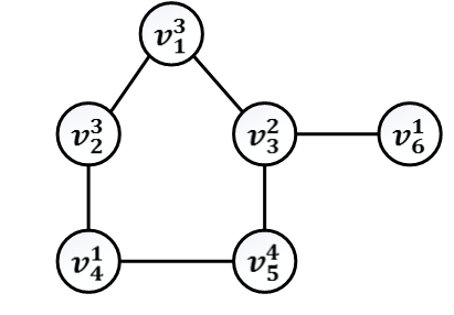
Figure 1: A vertex-weighted undirected graph $G$

Jiang et al. (2017)

Degree-1 Rule

For any vertex $v\in V$, if $w(v)\leq w(N_{1}(v))$, then $G^{\prime}=G\setminus N^{*}_{1}(v)$, and $S_{m}=S^{\prime}_{m}\cup\{v\}$.

Proof. Note that vertices in $N_{1}(v)$ do not have any neighbour other than $v$. Either $v$ or all vertices in $N_{1}(v)$ should be in a vertex cover of $G$ to cover the edges between $v$ and the vertices in $N_{1}(v)$. Since $w(v)\leq w(N_{1}(v))$, $S_{m}=S^{\prime}_{m}\cup\{v\}$ covers all edges of $G$ with minimum weight.

Example 2

Let $G=(V,E,w)$ be the vertex-weighted undirected graph of Figure 1 but the weight of $v_{6}$ is 3 (instead of 1). Since $N^{*}_{1}(v_{3})=\{v_{3},w_{6}\}$ and $w(v_{3})<w(v_{6})$, we can remove $v_{3}$ and $v_{6}$ from $G$ to obtain $G^{\prime}$. We then compute easily $S^{\prime}_{m}=\{v_{1},v_{4}\}$ for $G^{\prime}$ and $S_{m}=S^{\prime}_{m}\cup\{v_{3}\}=\{v_{1},v_{3},v_{4}\}$ for $G$. $\Box$

Degree-2 Rule

Let $A\subseteq V$ be a set of vertices with degree 2 that are all adjacent to vertices $v_{i}$ and $v_{j}$. If $w(v_{i})+w(v_{j})\leq w(A)$, then $G^{\prime}=G\setminus(A\cup\{v_{i},v_{j}\})$ and $S_{m}=S^{\prime}_{m}\cup\{v_{i},v_{j}\}$.

Proof. Note that there are no edges between any vertex in $A$ and any vertex other than $v_{i}$ and $v_{j}$ in $G$. It is easy to see that all edges that are in $G$ but not in $G^{\prime}$ are covered by $\{v_{i},v_{j}\}$. In addition, $w(v_{i})+w(v_{j})\leq w(A)$. Therefore, the set $S^{\prime}_{m}\cup\{v_{i},v_{j}\}$ covers all edges of $G$ and has minimum weight. $\Box$

Example 3

Let $G=(V,E,w)$ be the vertex-weighted undirected graph of Figure 1. Consider vertices $v_{3}$ and $v_{4}$ and $A=\{v_{5}\}$, because $v_{5}$ is adjacent to both $v_{3}$ and $v_{4}$ and has degree 2. Since $w(v_{3})+w(v_{4})<w(A)$, we can remove $v_{3}$, $v_{4}$ and $v_{5}$ from $G$ to obtain $G^{\prime}$. Then, $S^{\prime}_{m}=\{v_{1}\}$ is a minimum weight vertex cover of $G^{\prime}$ and $S_{m}=S^{\prime}_{m}\cup\{v_{3},v_{4}\}=\{v_{1},v_{3},v_{4}\}$ is a minimum weight vertex cover of $G$. $\Box$

Note that when $|N_{1}(v)|=1$ or $|A|=1$, Degree-1 Rule and Degree-2 Rule are equivalent to Adjacent Rule. To see this, let $N_{1}(v)=\{u\}$. Then, $N(u)=\{v\}$. So, $w(v)\leq w(N_{1}(v))$ is equivalent to $w(u)\geq w(N(u))$. Applying Adjacent Rule to $u$ is equivalent to applying Degree-1 Rule to $v$ in this case. The rules are different when $|N_{1}(v)|>1$ or $|A|>1$. For example, if $N_{1}(v)=\{u_{1},u_{2}\}$, $w(v)>w(u_{1})$, $w(v)>w(u_{2})$, but $w(v)\leq w(u_{1})+w(u_{2})$, Adjacent Rule is not applicable, but Degree-1 Rule is applicable.

Reduction Algorithm

We implemented Degree-0 Rule, Adjacent Rule, Degree-1 Rule and Degree-2 Rule in a reduction procedure to simplify $G$. The application of each rule results in a simplified graph $G^{\prime}$. Algorithm 1 shows the reduction procedure, which applies the rules in the ordering Degree-0 Rule, Adjacent Rule, Degree-1 Rule and Degree-2 Rule, each rule being repeatedly applied until it is no longer applicable. This ordering is chosen according to the increasing complexity of the rules.

Note that when a rule is applied after another rule, it can make the other rule applicable again. This is why the rule applications are implemented in a “do while” loop in Algorithm 1 to simplify as much as possible the graph. For example, when Degree-2 Rule is applied to remove $v_{3}$, $v_{4}$ and $v_{5}$ from $G$ in Figure 1 (See Example 3), the degree of $v_{6}$ becomes 0, enabling Degree-0 Rule. The loop stops when no rule is applicable. After using Algorithm 1, we obtain a simplified graph and a partial vertex cover, which is of great significance to the subsequent search.

Input: a graph $G=(V,E,w)$

Output: a reduced graph $G^{\prime}$ and a partial vertex cover $S$

1 begin

2       $S\leftarrow\emptyset$;

3      

4      do

5             $V^{\prime}\leftarrow V$;

6             while $v$ in $V$ satisfies Degree-0 Rule do

7                  $G\leftarrow$ Degree0Rule($G$);

8            while $v$ in $V$ satisfies Adjacent Rule do

9                  $G\leftarrow$ AdjacentRule($G$);

10                   move the vertices of $N(v)$ from $V$ to $S$;

11            while $v$ in $V$ satisfies Degree-1 Rule do

12                  $G\leftarrow$ Degree1Rule($G$);

13                   move $v$ from $V$ to $S$;

14            while $v_{i}$ and $v_{j}$ in $V$ satisfies Degree-2 Rule do

15                  $G\leftarrow$ Degree2Rule($G$);

16                   move $v_{i}$ and $v_{j}$ from $V$ to $S$;

17            

18      while $|V^{\prime}|\neq|V|$;

19      return $G[V^{\prime}]$ and $S$ ;

20      

21

Algorithm 1 Reduce($G$)

Input: a graph $G=(V,E,w)$

Output: A minimum weight vertex cover of $G$

1

2($G^{\prime},S$) $\leftarrow$ Reduce($G$);

3 Let $G^{\prime}$ consist of disjoint subgraphs $G_{1}=(V_{1},E_{1},w)$, $G_{2}=(V_{2},E_{2},w)$, …,$G_{k}=(V_{k},E_{k},w)$; /*$k\geq 1$*/

4 return $S$ $\cup$ Search$(G_{1},\emptyset,V_{1})$ $\cup$ Search$(G_{2},\emptyset,V_{2})$ $\cup\cdots\cup$ Search$(G_{k},\emptyset,V_{k})$;

Algorithm 2 BMWVC$(G)$

Input: a graph $G(V,E,w)$, a growing vertex cover $S$, the best vertex cover $S_{b}$ found so far

Output: a minimum weight vertex cover of $G$ extended from $S$

1

2if $G$ is empty then

3       return $S$;

4if LowerBound$(G)+w(S)\geq w(S_{b})$ then

5       return $S_{b}$;

6select a vertex $v$ from $G$ using a heuristic;

7 $S_{b}\leftarrow$ Search$(G\setminus\{v\},S\cup\{v\},S_{b})$;

8 return Search$(G\setminus N^{*}(v),S\cup N(v),S_{b})$;

Algorithm 3 Search$(G,S,S_{b})$

BMWVC: A Branch-and-Bound Algorithm for MWVC

In this section, we present our branch-and-bound algorithm BMWVC for MWVC, which is shown in Algorithm 2. Given a vertex-weighted graph $G$, BMWVC begins by simplifying $G$ using the reduction rules. The reduction produces a set of vertices $S$ that must be included in a minimum weight vertex cover of $G$, and can result in several disjoint subgraphs of $G$: $G_{1},G_{2},\ldots,G_{k}$ ($k\geq 1$). Then, BMWVC calls a Search procedure for each of the subgraph $G_{i}$ to independently searching for a minimum weight vertex cover of $G_{i}$. The union of these minimum weight vertex covers, together with $S$ and $S^{\prime}$, is returned as an optimal solution of $G$.

The Search procedure, showed in Algorithm 3, searches for a minimum weight vertex cover of $G$, beginning from an empty growing partial vertex cover $S$. It uses the best solution $S_{b}$ of $G$ found so far to prune search, because it should find a solution better than $S_{b}$ for $G$. For this purpose, it computes a lower bound of the best solution of $G$ and compares the lower bound with $S_{b}$. If the lower bound is smaller than the total weight of $S_{b}$, the search cannot be pruned and a vertex is chosen for branching. A minimum weight vertex cover of $G$ containing $\{v\}$ and another not containing $v$ (so, it should contain all vertices of $N(v)$) are respectively searched for, and the best one is returned. Note that a solution better than $S_{b}$ is returned only when $G$ becomes empty in a recursive call, because only in this case, the search was not pruned because of $S_{b}$. In all other cases, the Search procedure returns $S_{b}$.

There are two crucial components in the Search procedure. The first component is a branching heuristic that selects a vertex $v$ and implicitly divide the set of all vertex covers of $G$ into the subset of vertex covers that contain $v$ and the subset of vertex covers that do not contain $v$. In the first case, the search continue to search for a minimum weight vertex cover of $G\setminus\{v\}$, and in the second case, the vertices in $N(v)$ should be in the vertex covers in the subset and the search continue to search for a minimum weight vertex cover of $G\setminus N^{*}(v)$.

The branching heuristic is important because it may impact greatly on the search tree size. We consider the following four heuristic strategies related to degree and weight of a vertex.

• H1: select a vertex $v$ from $V$ with the greatest $d(v)$.

• H2: select a vertex $v$ from $V$ randomly.

• H3: select a vertex $v$ from $V$ with the smallest $w(v)$.

• H4: select a vertex $v$ from $V$ with the greatest $d(v)/$ $w(v)$.

The reason why we take degree and weight as the heuristic factors is that more vertices and edges can be deleted after a vertex with the greater $d(v)$ is selected, which can reduce the size of the explored search tree. In addition, since the aim of the MWVC problem is to find a minimum weight vertex cover, we prefer to select a vertex with a smaller weight. When there are more than one vertex as candidates, we select a vertex $v$ with the smallest number of edges whose endpoints are both in $N(v)$.

The second component of BMWVC is a lower bound of $S_{m}$, which is essential to reduce the search space. If the weight of current partial vertex cover plus the lower bound is equal to or bigger than the weight of the best solution found so far, we can prune the current subtree. The tighter the lower bound is, the more search space can be pruned. BMWVC adopts an easy and natural method to calculate the lower bound. It partitions $G$ into a set of disjoint cliques $C_{1}$, $C_{2}$, …,$C_{n}$. Then LowerBound(G) $=\sum\limits_{i=1}^{n}(w(C_{i})-\max\limits_{v_{j}\in C_{i}}(w(v_{j})))$, because $k-1$ vertices are needed to cover all edges of a clique of $k$ vertices.

Table 1: Runtimes in seconds of 4 branching heuristics for a set of graphs. The cut-off time is 1000 seconds

Instance	H1	H2	H3	H4
bio-celegans	0.604	-	-	-
bio-diseasome	0.031	29.946	10.322	0.553
bio-yeast	0.005	0.008	0.008	0.007
bn-macaque-rhesus-brain-2	0.001	0.001	0.001	0.001
boyd2	0.703	-	-	-
ca-CSphd	0.007	0.007	0.007	0.006
ca-Erdos992	0.006	0.006	0.007	0.007
ca-netscience	0.025	265.614	52.346	0.530
can-96	0.104	1.435	1.102	0.019
com-youtube	0.092	0.097	0.097	0.099
dwt-59	0.251	0.153	0.717	0.137
gent113	0.017	0.290	0.161	0.017
GD95-c	0.017	0.073	0.066	0.030
ia-email-EU	0.029	0.029	0.029	0.030
ia-enron-only	0.568	-	-	52.192
ia-reality	0.011	0.011	0.011	0.012
inf-contiguous-usa	0.013	0.025	0.083	0.026
lp1	0.328	0.344	0.361	0.292
opsahl-southernwomen	0.003	0.002	0.002	0.001
road-chesapeake	0.003	0.012	0.026	0.008
rt-retweet	0.002	0.030	0.003	0.003
rt-retweet-crawl	0.545	18.811	19.172	3.325
rt-twitter-copen	0.005	0.005	0.004	0.005
soc-dolphins	0.007	0.043	0.029	0.020
soc-douban	0.149	0.122	0.123	0.122
soc-gplus	0.023	0.022	0.022	0.030
soc-karate	0.002	0.002	0.002	0.001
tech-as-caida2007	0.036	0.068	0.086	0.048
web-edu	0.055	0.076	0.108	0.047
web-indochina-2004	2.572	-	-	-
web-google	0.031	0.150	0.006	0.061
web-polblogs	0.829	-	-	-
web-webbase-2001	0.566	-	-	-

Experiments

In this section, we evaluate our BMWVC on real-world massive graphs from Network Data Repository Rossi and Ahmed (2015), which are used to evaluate MWVC and MWC problems in Cai et al. (2018); Jiang et al. (2017) and the graphs from practical applications McCreesh et al. (2017). The weights in the first dataset are assigned $w(v_{i})=(i+1)\ mod\ 200$ to each vertex $v_{i}$ as in Cai et al. (2018); Jiang et al. (2017). The weights in the second dataset represent real meanings. We implement our algorithm BMWVC in Java and compile it using jdk (version 1.7). The experiments are carried out on a workstation under CentOS Linux, using 12 core Intel(R) Xeon(R) E5-2650 v4 2.20 GHz CPU and 128 GB RAM. In all experiments, the runtimes are in seconds and “-” means timeout or out of memory.

Heuristic Selection

In the subsection, we test four heuristic strategies H1, H2, H3, and H4 described above to select the best one. Table 1 shows the running time of the four heuristic strategies with a cut-off time of 1000 seconds. From the table, we can find that H1 performs the best on most instances. In contrast, H2, H3 and H4 fail to solve more than 5 instances, which can be solved by H1 very easily. On the whole, H1 is the best heuristic strategy and we select it as the branching heuristic of BMWVC in all subsequent experiments.

Table 2: Remaining number of vertices after applying one or several reduction rules to a graph. The last column gives the number of subgraphs after applying all reduction rules in $R_{a12}$

Instance	$|V|$	$R_{a}$	$R_{a12}$	$N_{G}$
bio-celegans	453	422	419	1
bio-diseasome	516	335	303	13
bio-yeast	1458	297	118	18
bn-macaque-rhesus-brain-2	91	0	0	0
boyd2	466316	140180	120666	1
ca-CSphd	1882	394	77	14
ca-Erdos992	5094	429	0	0
ca-netscience	379	275	257	22
can-96	96	96	96	1
com-youtube	6320737	653	0	0
dwt59	59	51	51	1
ia-email-EU	32430	605	0	0
ia-enron-only	143	138	138	1
ia-reality	6809	0	0	0
inf-contiguous-usa	49	42	42	1
GD95-c	62	62	62	1
gent113	113	104	104	1
lp1	534388	5115	2831	320
opsahl-southernwomen	18	18	18	1
road-chesapeake	39	39	39	1
rt-retweet-crawl	1112702	89603	2309	289
rt-retweet	96	24	5	1
rt-twitter-copen	761	248	65	13
soc-dolphins	62	50	50	1
soc-douban	154908	26164	38	4
soc-gplus	23628	115	0	0
soc-karate	34	20	8	1
tech-as-caida2007	26475	2657	272	46
web-edu	3031	1177	985	28
web-indochina-2004	11358	9280	9026	483
web-google	1299	516	363	24
web-polblogs	643	255	194	1
web-webbase-2001	16062	3141	1996	76

Effectiveness of Reduction Rules

To evaluate the effectiveness of the proposed reduction rules, we implemented two different reduction algorithms: $R_{a}$ and $R_{a12}$. Specially, $R_{a}$ employs Adjacent reduction and $R_{a12}$ use Adjacent Rule, Degree-1 Rule and Degree-2 Rule and is exactly Algorithm 1. Note that the trivial Degree-0 rule is executed in all reduction algorithms.

Table 2 shows the remaining vertices after performing the three reduction algorithms to simplify a set of graphs. Since the application of these reduction rules to a graph can result in several subgraphs, we also count the number of subgraphs, denoted by $N_{G}$ after applying $R_{a12}$. From the table, we see that reduction rules are effective. Comparing the size of the graph after the reduction, we find $R_{a12}$ produces smaller graphs than $R_{a}$.

We also studied the effectiveness of our reduction rules. Figure 2 compares BMWVC and OBMWVC, a variant of BMWVC without using any reduction rule. It is easy to see from Figure 2 that BMWVC is much faster than OBMWVC.

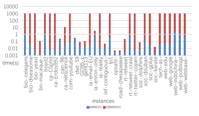
Figure 2: Runtimes of BMWVC(blue) and OBMWVC(red)

Table 3: Experimental results in large spare graphs

Instance	$S_{m}$	BMWVC	WLMC	SBMS	Dynwvc1/Dynwvc2
					best	avgt
bio-celegans	20099	0.60	6.04	-	20100$\uparrow$	0.03
bio-diseasome	22205	0.03	377.82	-	22205	<0.01
bio-yeast	36168	<0.01	-	-	36168	<0.01
bn-macaque-rhesus-brain-2	284	<0.01	0.15	-	284	<0.01
boyd2	17025951	0.70	-	-	17032631$\uparrow$	0.71
ca-CSphd	48899	<0.01	-	-	48899	0.02
ca-dblp-2010	15636204*	90.41*	-	-	12156739	966.98
ca-dblp-2012	19995803*	127.29*	-	-	15026140	988.05
ca-Erdos992	40710	<0.01	-	-	41110 $\uparrow$	<0.01
ca-netscience	19292	0.03	0.50	201.88	19292	<0.01
can-96	3360	0.10	0.19	7.37	3360	<0.01
com-youtube	58549	0.09	-	-	58549	0.71
dwt59	1031	0.25	0.16	3.58	1031	<0.01
GD95-c	1215	0.02	0.16	3.63	1215	<0.01
gent113	3152	0.02	0.15	12.30	3152	<0.01
ia-email-EU	78310	0.03	-	-	78311$\uparrow$	<0.01
ia-enron-only	5988	0.57	0.27	-	5988	<0.01
ia-reality	3601	0.01	-	-	3601	<0.01
inf-contiguous-usa	741	0.01	0.14	3.39	741	<0.01
inf-roadNet-CA	194721905*	0.0*	-	-	97206712	999.92
inf-roadNet-PA	68980405*	986.45*	-	-	53268783	416.69
lp1	24165495	0.33	-	-	24190047$\uparrow$	103.32
opsahl-southernwomen	97	<0.01	0.24	3.07	97	<0.01
rec-amazon	4071861	17.56	-	-	4121394$\uparrow$	813.93
road-chesapeake	446	<0.01	0.14	3.22	446	<0.01
rt-retweet	1339	<0.01	0.15	10.16	1339	<0.01
rt-retweet-crawl	7821627	0.55	-	-	7821858$\uparrow$	816.47
rt-twitter-copen	19353	<0.01	-	-	19353	<0.01
soc-dolphins	969	<0.01	0.14	5.41	969	<0.01
soc-douban	857460	0.15	-	-	857462$\uparrow$	1.70
soc-flixster	9428344	1.21	-	-	9529398$\uparrow$	740.35
soc-FourSquare	63580619*	0.0*	-	-	8768847	812.02
soc-gplus	12406	0.02	-	-	12406	0.03
soc-karate	226	<0.01	0.02	3.14	226	<0.01
soc-lastfm	7698963	0.92	-	-	7778530$\uparrow$	471.64
soc-twitter-follows	231887	0.19	-	-	234249$\uparrow$	1.06
socfb-A-anon	308165360*	0.0*	-	-	37022624	188.89
socfb-B-anon	29555630	4.85	-	-	29901404$\uparrow$	999.61
tech-as-caida2007	310840	0.04	-	-	310860$\uparrow$	50.26
tech-internet-as	487337	0.06	-	-	492656$\uparrow$	61.57
tech-ip	6653664	1.48	-	-	6653664	720.43
web-edu	138214	0.06	-	-	138214	0.03
web-indochina-2004	713983	2.57	-	-	714003$\uparrow$	268.00
web-google	41511	0.03	-	-	41511	0.02
web-polblogs	20093	0.83	-	-	20093	<0.01
web-webbase-2001	254341	0.57	-	-	254343$\uparrow$	75.93
web-wikipedia2009	185508394*	0.0*	-	-	57518328	330.00

Comparison in Large Spare Graphs

We conducted an experiment on real-world large graphs to compare BMWVC with WLMC Jiang et al. (2017), the most competitive exact solver for MWC, SBMS Xu et al. (2016), a solver encoding MWVC into SAT, Dynwvc1 and Dynwvc2 Cai et al. (2018), two best heuristic MWVC solvers. The cut-off time of all solvers is 1000 seconds. For MWC solver WLMC, we execute it for the complementary graphs. For the sake of space, we only show the results on the 47 graphs with $|E|/|V|$ less than 7.

Table 3 indicates runtimes of the five solvers. The first column gives the name of the graphs. The second column $S_{m}$ gives the solutions MWVC of these graphs found by BMWVC. BMWVC proved the optimality of these solutions, except those marked by “*”, where “*” indicates that BMWVC encountered memory overflow and stopped the search and that the corresponding solutions are the best solutions found by BMWVC before memory overflow. The next three columns gives the runtimes of BMWVC, WLMC and SBMC. The last two columns give the best solutions found by two heuristics Dynwvc1 and Dynwvc2 over the 10 independent runs (the cut-off time of each run is 1000 seconds) and the mean time to reach the best solution in each run (avgt), “$\uparrow$” indicating that the heuristic algorithms don’t find the optimal solution. The best times are in bold (for heuristic solvers, times are not in bold if the best weight found is not optimal or has not been proved to be optimal by an exact solver).

From table 3, we observe that BMWVC finds the optimum for most graphs, while Dynwvc1 and Dynwvc2 fail to find the optimum on 16 instances; WLMC and SBMS fail to solve more than 32 instances. Surprisingly, BMWVC needs less time than heuristic solvers on 17 instances to find and prove the optimal solution. In general, these results indicate that BMWVC is an extremely competitive exact solver.

Comparison in Application Graphs

We also compare our BMWVC with MLMC, SBMS, Dynwvc1, and Dynwvc2 in application graphs, whose densities (($2*|E|)/(|V|*(|V|-1))$) range from 0.04 to 0.98. These graphs, which are used to evaluate MWC solvers in Jiang et al. (2018); Hebrard and Katsirelos (2018), are derived from four important practical problems: the winner determination problem (WDP), error-correcting codes (ECC), kidney-exchange schemes (KES), and the research excellence framework (REF). Table 4 indicates the number of successfully solved instances grouped by families within a cut-off time of 5 hours for exact solvers and heuristic solvers, where “$\#$” is the total instances of each family. Note that the MWVC solvers BMWVC, SBMS, Dynwvc1, and Dynwvc2 are performed on the complementary graphs.

From Table 4, it is easy to see that BMWVC performs significantly better than SBMS, Dynwvc1 and Dynwvc2. It performs slightly less well than WLMC, because these graphs arise from MWC practical applications, and some of them are too sparse so that the complementary graphs are too dense for all MWVC solvers. The purpose of this experiment is to show that BMWVC is competitive even for these applications not exactly in its field and is substantially better than other MWVC solving approaches.

Table 4: The number of solved graphs

Instance	$\#$	BMWVC	WLMC	SBMS	Dyn1/Dyn2
WDP	50	50	50	10	39
KES	100	89	100	71	27
ECC	15	13	15	1	15
REF	128	103	104	4	128
total	293	255	269	86	209

Conclusions

We proposed BMWVC, a new exact MWVC algorithm, which involves four reduction rules, a tight lower bound, and an efficient branching heuristic. The reported experiments show that the reduction rules are very effective in reducing massive graphs to tractable sizes; the tight lower bound can successfully prune search; and the efficient branching heuristic greatly decreases the running time. They also show that BMWVC outperforms relevant exact and heuristic MWVC solving approaches for real-world large graphs and application instances.

References

- Akiba and Iwata [2016] Takuya Akiba and Yoichi Iwata. Branch-and-reduce exponential/fpt algorithms in practice: A case study of vertex cover. Theoretical Computer Science, 609:211–225, 2016.
- Balachandar and Kannan [2009] S Raja Balachandar and K Kannan. A meta-heuristic algorithm for vertex covering problem based on gravity. International Journal of Mathematical and Statistical Sciences, 1(3):130–136, 2009.
- Balaji et al. [2010] S Balaji, V Swaminathan, and K Kannan. An effective algorithm for minimum weighted vertex cover problem. Int. J. Comput. Math. Sci, 4:34–38, 2010.
- Benlic and Hao [2013] Una Benlic and Jin-Kao Hao. Breakout local search for the max-cutproblem. Engineering Applications of Artificial Intelligence, 26(3):1162–1173, 2013.
- Bouamama et al. [2012] Salim Bouamama, Christian Blum, and Abdellah Boukerram. A population-based iterated greedy algorithm for the minimum weight vertex cover problem. Applied Soft Computing, 12(6):1632–1639, 2012.
- Cai et al. [2018] Shaowei Cai, Wenying Hou, Jinkun Lin, and Yuanjie Li. Improving local search for minimum weight vertex cover by dynamic strategies. In IJCAI, pages 1412–1418, 2018.
- Garey [1979] Michael R Garey. A guide to the theory of np-completeness. Computers and intractability, 1979.
- Hebrard and Katsirelos [2018] Emmanuel Hebrard and George Katsirelos. Conflict directed clause learning for maximum weighted clique problem. In IJCAI, pages 1316–1323, 2018.
- Iwata et al. [2014] Yoichi Iwata, Keigo Oka, and Yuichi Yoshida. Linear-time fpt algorithms via network flow. In Proceedings of the twenty-fifth annual ACM-SIAM symposium on Discrete algorithms, pages 1749–1761. Society for Industrial and Applied Mathematics, 2014.
- Jiang et al. [2017] Hua Jiang, Chu-Min Li, and Felip Manya. An exact algorithm for the maximum weight clique problem in large graphs. In AAAI, pages 830–838, 2017.
- Jiang et al. [2018] Hua Jiang, Chu-Min Li, Yanli Liu, and Felip Manyà. A two-stage maxsat reasoning approach for the maximum weight clique problem. In AAAI, 2018.
- Jovanovic and Tuba [2011] Raka Jovanovic and Milan Tuba. An ant colony optimization algorithm with improved pheromone correction strategy for the minimum weight vertex cover problem. Applied Soft Computing, 11(8):5360–5366, 2011.
- Kratsch et al. [2009] Kratsch, Stefan, Neumann, and Frank. Fixed-parameter evolutionary algorithms and the vertex cover problem. 2009.
- Li et al. [2016] Ruizhi Li, Shuli Hu, Haochen Zhang, and Minghao Yin. An efficient local search framework for the minimum weighted vertex cover problem. Information Sciences, 372:428–445, 2016.
- Li et al. [2018] Ruizhi Li, Shaowei Cai, Shuli Hu, Minghao Yin, and Jian Gao. Numwvc: A novel local search for minimum weighted vertex cover problem. In AAAI, 2018.
- Ma and Jan Latecki [2013] Tianyang Ma and Longin Jan Latecki. Graph transduction learning with connectivity constraints with application to multiple foreground cosegmentation. In Proceedings of the IEEE Conference on Computer Vision and Pattern Recognition, pages 1955–1962, 2013.
- Mascia et al. [2010] Franco Mascia, Elisa Cilia, Mauro Brunato, and Andrea Passerini. Predicting structural and functional sites in proteins by searching for maximum-weight cliques. In AAAI, 2010.
- McCreesh et al. [2017] Ciaran McCreesh, Patrick Prosser, Kyle Simpson, and James Trimble. On maximum weight clique algorithms, and how they are evaluated. In International Conference on Principles and Practice of Constraint Programming, pages 206–225. Springer, 2017.
- Nakajima et al. [2018] Masaru Nakajima, Hong Xu, and Sven Koenig TK Satish Kumar. Towards understanding the min-sum message passing algorithm for the minimum weighted vertex cover problem: An analytical approach. In The International Symposium on Artificial Intelligence and Mathematics, page 1, 2018.
- Newman [2003] Mark EJ Newman. The structure and function of complex networks. SIAM review, 45(2):167–256, 2003.
- Niedermeier and Rossmanith [2003] Rolf Niedermeier and Peter Rossmanith. On efficient fixed-parameter algorithms for weighted vertex cover. Journal of Algorithms, 47(2):63–77, 2003.
- Rossi and Ahmed [2015] Ryan A. Rossi and Nesreen K. Ahmed. The network data repository with interactive graph analytics and visualization. In Proceedings of the Twenty-Ninth AAAI Conference on Artificial Intelligence, 2015.
- Shyu et al. [2004] Shyong Jian Shyu, Peng-Yeng Yin, and Bertrand MT Lin. An ant colony optimization algorithm for the minimum weight vertex cover problem. Annals of Operations Research, 131(1-4):283–304, 2004.
- Tang et al. [2017] Changbing Tang, Ang Li, and Xiang Li. Asymmetric game: A silver bullet to weighted vertex cover of networks. IEEE transactions on cybernetics, 2017.
- Wang et al. [2015] Limin Wang, Xiaoyan Zhang, Zhao Zhang, and Hajo Broersma. A ptas for the minimum weight connected vertex cover p3 problem on unit disk graphs. Theoretical computer science, 571:58–66, 2015.
- Wang et al. [2017] Limin Wang, Wenxue Du, Zhao Zhang, and Xiaoyan Zhang. A ptas for minimum weighted connected vertex cover p 3 problem in 3-dimensional wireless sensor networks. Journal of Combinatorial Optimization, 33(1):106–122, 2017.
- Xu and Ma [2006] Xinshun Xu and Jun Ma. An efficient simulated annealing algorithm for the minimum vertex cover problem. Neurocomputing, 69(7-9):913–916, 2006.
- Xu et al. [2016] Hong Xu, TK Satish Kumar, and Sven Koenig. A new solver for the minimum weighted vertex cover problem. In International Conference on AI and OR Techniques in Constriant Programming for Combinatorial Optimization Problems, pages 392–405. Springer, 2016.
- Zhian et al. [2013] Hootan Zhian, Masoud Sabaei, Nastooh Taheri Javan, and Omid Tavallaie. Increasing coding opportunities using maximum-weight clique. In Computer Science and Electronic Engineering Conference (CEEC), 2013 5th, pages 168–173. IEEE, 2013.
- Zhou et al. [2016] Taoqing Zhou, Zhipeng Lü, Yang Wang, Junwen Ding, and Bo Peng. Multi-start iterated tabu search for the minimum weight vertex cover problem. Journal of Combinatorial Optimization, 32(2):368–384, 2016.