Semileptonic decays of the scalar tetraquark $Z_{bc;\overline{u}\overline{d}}^{0}$

Abstract

We study semileptonic decays of the scalar tetraquark $Z_{bc;\overline{u}\overline{d}}^{0}$ to final states $T_{bs;\overline{u}\overline{d}}^{-}e^{+}\nu_{e}$ and $T_{bs;\overline{u}\overline{d}}^{-}\mu^{+}\nu_{\mu}$, which run through the weak transitions $c\to se^{+}\nu_{e}$ and $c\to s\mu^{+}\nu_{\mu}$, respectively. To this end, we calculate the mass and coupling of the final-state scalar tetraquark $T_{bs;\overline{u}\overline{d}}^{-}$ by means of the QCD two-point sum rule method: these spectroscopic parameters are used in our following investigations. In calculations we take into account the vacuum expectation values of the quark, gluon, and mixed operators up to dimension ten. We use also three-point sum rules to evaluate the weak form factors $G_{i}(q^{2})$ ($i=1,~{}2$) that describe these decays. The sum rule predictions for $G_{i}(q^{2})$ are employed to construct fit functions $F_{i}(q^{2})$, which allow us to extrapolate the form factors to the whole region of kinematically accessible $q^{2}$. These functions are required to get partial widths of the semileptonic decays $\Gamma\left(Z_{bc}^{0}\rightarrow Te^{+}\nu_{e}\right)$ and $\Gamma\left(Z_{bc}^{0}\rightarrow T\mu^{+}\nu_{\mu}\right)$ by integrating corresponding differential rates. We analyze also the two-body nonleptonic decays $Z_{bc;\overline{u}\overline{d}}^{0}\to T_{bs;\overline{u}\overline{d}}^{-}\pi^{+}$ and $Z_{bc;\overline{u}\overline{d}}^{0}\to T_{bs;\overline{u}\overline{d}}^{-}K^{+}$, which are necessary to evaluate the full width of the $Z_{bc;\overline{u}\overline{d}}^{0}$. The obtained results for $\Gamma_{\mathrm{full}}=(3.18\pm 0.39)\times 10^{-11}~{}\mathrm{MeV}$ and mean lifetime $20.7_{-2.3}^{+2.9}~{}\mathrm{ps}$ of the tetraquark $Z_{bc;\overline{u}\overline{d}}^{0}$ can be used in experimental investigations of this exotic state.

I Introduction

Investigations of double-heavy tetraquarks composed of a heavy $QQ$ diquark [$Q$ is the heavy $c$ or $b$ quark] and a light antidiquark are among interesting topics in physics of exotic hadrons. The interest to such kind of quark configurations is connected with a possible stability of some of them against the strong and electromagnetic decays. The relevant problems were addressed already in the pioneering papers Ader:1981db ; Lipkin:1986dw ; Zouzou:1986qh , in which a stability of the exotic four-quark mesons $QQ\bar{Q}\bar{Q}$ and $QQ\bar{q}\bar{q}$ was examined. It was found that the heavy $Q$ and light $q$ quarks with a large mass ratio $m_{Q}/m_{q}$ may form the stable tetraquarks $QQ\bar{q}\bar{q}$. The similar conclusions were drawn in Ref. Carlson:1987hh as well, in accordance of which the isoscalar $J^{P}=1^{+}$ tetraquark $T_{bb;\overline{u}\overline{d}}^{-}$ lies below the two B-meson threshold and can decay only weakly.

All available theoretical tools of high energy physics were exploited to study properties of double-heavy exotic mesons; the chiral and dynamical quark models, the relativistic quark model and sum rules method were mobilized to calculate their parameters Pepin:1996id ; Janc:2004qn ; Cui:2006mp ; Vijande:2006jf ; Ebert:2007rn ; Navarra:2007yw ; Du:2012wp ; Hyodo:2012pm ; Esposito:2013fma . Interest to these mesons renewed after experimental observation by the LHCb Collaboration of the $\Xi_{cc}^{++}=ccu$ baryon Aaij:2017ueg . Its mass was used as an input information in a phenomenological model to estimate the mass of the axial-vector tetraquark $T_{bb;\overline{u}\overline{d}}^{-}$ Karliner:2017qjm . The obtained prediction $m=(10389\pm 12)~{}\mathrm{MeV}$ is $215~{}\mathrm{MeV}$ below the $B^{-}\overline{B}^{\ast 0}$ threshold and $170~{}\mathrm{MeV}$ below the threshold for decay $B^{-}\overline{B}^{0}\gamma$, which means that $T_{bb;\overline{u}\overline{d}}^{-}$ is stable against the strong and electromagnetic decays and dissociates only weakly. The conclusion about the strong-interaction stability of the tetraquarks $T_{bb;\overline{u}\overline{d}}^{-}$, $T_{bb;\overline{u}\overline{s}}^{-}$, and $T_{bb;\overline{d}\overline{s}}^{0}$ was made in Ref. Eichten:2017ffp on the basis of the relations derived from heavy-quark symmetry. The mass $m=10482~{}\mathrm{MeV}$ of the axial-vector tetraquark $T_{bb;\overline{u}\overline{d}}^{-}$ found there is $121~{}\mathrm{MeV}$ below the open-bottom threshold.

In Ref. Agaev:2018khe we calculated the spectroscopic parameters of the axial-vector tetraquark $T_{bb;\overline{u}\overline{d}}^{-}$ and analyzed also its semileptonic decay to the scalar state $Z_{bc;\overline{u}\overline{d}}^{0}$. Our result for its mass $m=(10035~{}\pm 260)~{}\mathrm{MeV}$ confirms once more that it is stable against the strong and electromagnetic decays. We evaluated the total width and mean lifetime of $T_{bb;\bar{u}\bar{d}}^{-}$  using the semileptonic decay channels $T_{bb;\overline{u}\overline{d}}^{-}\rightarrow Z_{bc;\overline{u}\overline{d}}^{0}l\bar{\nu_{l}}$, where $l=e,\mu$ and $\tau$. The predictions $\Gamma=(7.17\pm 1.23)\times 10^{-8}~{}\mathrm{MeV}$ and $\tau=9.18_{-1.34}^{+1.90}~{}\mathrm{fs}$ provide information useful for experimental investigation of the double-heavy exotic mesons. Details of performed analysis and references to earlier and recent articles devoted to different aspects of the doubly and fully heavy tetraquarks can be found in Ref. Agaev:2018khe .

We determined the mass and coupling of the scalar four-quark meson $Z_{bc;\overline{u}\overline{d}}^{0}$ (hereafter $Z_{bc}^{0}$) as well Agaev:2018khe , because these parameters were necessary to evaluate the width of the semileptonic decay $T_{bb;\overline{u}\overline{d}}^{-}\rightarrow Z_{bc}^{0}l\bar{\nu_{l}}$. For these purposes we employed the QCD sum rule approach and found $m_{Z}=(6660\pm 150)~{}\mathrm{MeV}$. This prediction is considerably below the threshold $7145~{}\mathrm{MeV}$ for strong decays of $Z_{bc}^{0}$ to heavy mesons $B^{-}D^{+}$ and $\overline{B^{0}}D^{0}$. The state $Z_{bc}^{0}$ cannot decay to a pair of heavy and light mesons as well; this fact differs it qualitatively from the open charm-bottom scalar tetraquarks $cq\overline{b}\overline{q}$ and $cs\overline{b}\overline{s}$, which decay to $B_{c}\pi$ and $B_{c}\eta$ mesons Agaev:2016dsg , respectively. The thresholds for the electromagnetic decays $Z_{bc}^{0}\rightarrow\overline{B^{0}}D_{1}^{0}\gamma$ and $B^{\ast}D_{0}^{\ast}\gamma$ exceed $7600~{}\mathrm{MeV}$ and are higher than the mass of $Z_{bc}^{0}$. In other words, the tetraquark $Z_{bc}^{0}$ as the state $T_{bb;\bar{u}\bar{d}}^{-}$ is the strong- and electromagnetic-interaction stable particle.

The scalar and axial-vector states $bc\overline{u}\overline{d}$ were subjects of interesting theoretical investigations with, sometimes, controversial predictions. In fact, the analysis performed in Ref. Karliner:2017qjm showed that $Z_{bc}^{0}$ resides $11~{}\mathrm{MeV}$ below the threshold $7145~{}\mathrm{MeV}$ for $S$-wave decays to conventional heavy $B^{-}D^{+}$ and $\overline{B^{0}}D^{0}$ mesons. Computations of the ground-state $QQ^{\prime}\overline{u}\overline{d}$ tetraquarks’ masses carried out in the context of the Bethe-Salpeter method led to similar conclusions Feng:2013kea . The mass of $Z_{bc}^{0}$ found there (for some set of used parameters) equals to $6.93~{}\mathrm{GeV}$ and is lower than the relevant strong threshold. On the contrary, for the masses of the scalar and axial-vector $bc\overline{u}\overline{d}$ states the heavy-quark symmetry predicts $7229~{}\mathrm{MeV}$ and $7272~{}\mathrm{MeV}$ Eichten:2017ffp , which means that they can decay to ordinary mesons $B^{-}D^{+}/\overline{B^{0}}D^{0}$ and $B^{\ast}D$, respectively. The charged exotic scalar mesons $Z_{bc;\overline{u}\overline{u}}^{-}$ and $Z_{bc;\overline{d}\overline{d}}^{+}$ were explored by means of the QCD sum rule method as well Chen:2013aba ; the mass of these particles $m=(7.14\pm 0.10)~{}\mathrm{GeV}$ is higher than our prediction for $m_{Z}$.

The recent lattice simulations prove the strong-interaction stability of the $I(J^{P})=0(1^{+})$ four-quark meson $Z_{ud;\overline{c}\overline{b}}^{0}$ with the mass in the range $15$ to $61$ $\mathrm{MeV}$ below $\overline{D}B^{\ast}$ threshold Francis:2018jyb . But, because of theoretical uncertainties the authors could not determine whether this tetraquark would decay electromagnetically to $\overline{D}B\gamma$ or can transform only weakly. Another confirmation of the $bc\overline{u}\overline{d}$ tetraquarks stability came from Ref. Caramees:2018oue ; there it was demonstrated that both the $J^{P}=0^{+}$ and $1^{+}$ isoscalar tetraquarks $bc\overline{u}\overline{d}$ are stable against the strong decays. The isoscalar $J^{P}=0^{+}$ state is also electromagnetic-interaction stable, whereas $J^{P}=1^{+}$ may undergo the electromagnetic decay to $\overline{B}D\gamma$.

In light all of these theoretical predictions, it becomes evident that decays of the tetraquark $Z_{bc}^{0}$ are sources of a valuable information about this exotic meson. In the present work we explore the semileptonic decays of the tetraquark $Z_{bc}^{0}$ which are important for some reasons. First of all, $Z_{bc}^{0}$ may be produced copiously at the LHC Ali:2018xfq , hence it is necessary to fix processes, where it has to be searched for. The second reason is exploration of the tetraquark $T_{bb;\overline{u}\overline{d}}^{-}$ itself, and decay channels appropriate for its discovery. As usual, all states classified till now as candidates to tetraquarks were seen through their decays to conventional mesons. If a tetraquark is stable against strong and electromagnetic decays, then it should be observed due to products of its weak decays. In the case under discussion at the first stage $T_{bb;\overline{u}\overline{d}}^{-}$ decays to $Z_{bc}^{0}$ and $l\bar{\nu_{l}}$. But, because the scalar tetraquark $Z_{bc}^{0}$ does not transform directly to conventional mesons, one needs to consider its weak decays, as well.

The weak decays of $Z_{bc}^{0}$ can proceed through different channels. The dominant semileptonic decay modes of $Z_{bc}^{0}$ are the processes $Z_{bc}^{0}\rightarrow T_{bs;\overline{u}\overline{d}}^{-}e^{+}\nu_{e}$ and $Z_{bc}^{0}\rightarrow T_{bs;\overline{u}\overline{d}}^{-}\mu^{+}\nu_{\mu}$, which run due to transitions $c\rightarrow W^{+}s$ and $W^{+}\rightarrow\overline{l}\nu_{l}$. The channels triggered by the decays $c\rightarrow W^{+}d$ and $W^{+}\rightarrow\overline{l}\nu_{l}$ lead to creation of the tetraquark $T_{bd;\overline{u}\overline{d}}^{-}$, and are suppressed relative to the first modes by a factor $|V_{cd}|^{2}/|V_{cs}|^{2}\simeq 0.05$. The similar arguments can be applied to other semileptonic decays of $Z_{bc}^{0}$ generated by a chain of transitions $b\rightarrow W^{-}c$ $\rightarrow cl\overline{\nu}_{l}$ and $b\rightarrow W^{-}u$ $\rightarrow ul\overline{\nu}_{l}$, respectively. In fact, the Cabibbo-Kobayashi-Maskawa (CKM) matrix element $|V_{bc}|$, which is small numerically, and the ratio $|V_{bu}|^{2}/|V_{bc}|^{2}$ $\simeq 0.01$ demonstrates a subdominant nature of the decays $b\rightarrow cl\overline{\nu}_{l}$ and $b\rightarrow ul\overline{\nu}_{l}$. The weak decay $c\rightarrow W^{+}s$ may be followed by transitions $W^{+}\rightarrow u\overline{d}$ and $W^{+}\rightarrow u\overline{s}$, which give rise to nonleptonic decays of $Z_{bc}^{0}$. In the hard-scattering mechanism, for example, a pair $u\overline{d}$ may form ordinary mesons with $q\overline{q}$ quarks appeared due to a gluon from one of $u$ or $\overline{d}$ quarks. These processes lead to final states $Z_{bc}^{0}\rightarrow T_{bs;\overline{u}\overline{d}}^{-}M_{1}(u\overline{q})M_{2}(q\overline{d})$ which are suppressed relative to the semileptonic decays by the factor $\alpha_{s}^{2}|V_{ud}|^{2}$. But $u\overline{d}$ and $u\overline{s}$ quarks can form $\pi^{+}$ and $K^{+\text{ }}$mesons and generate the two-body nonleptonic decays of the tetraquark $Z_{bc}^{0}$, i.e., the processes $Z_{bc}^{0}\rightarrow T_{bs;\overline{u}\overline{d}}^{-}\pi^{+}$ and $Z_{bc}^{0}\rightarrow T_{bs;\overline{u}\overline{d}}^{-}K^{+}$ . There is also a class of multimeson processes, when $u\overline{d}$ and $u\overline{s}$ combine directly with quarks from $T_{bs;\overline{u}\overline{d}}^{-}$ and create three-meson final states. The two-body and three-meson nonleptonic decays do not suppressed by additional factors relative to the semileptonic decays, and their contributions to full width of $Z_{bc}^{0}$ may be sizeable. Parameters of these channels may provide a valuable new information on features of the exotic meson $Z_{bc}^{0}$.

The tetraquark $T_{bs;\overline{u}\overline{d}}^{-}$ can bear different quantum numbers. We treat $T_{bs;\overline{u}\overline{d}}^{-}$ as a scalar particle, and in what follows denote it by $T$ . To calculate the width of aforementioned decays, one needs the mass and coupling of the tetraquark $T$ ; they enter as parameters to the sum rules for the weak form factors that determine width of the decays. The spectroscopic parameters of this tetraquark can be extracted from the two-point correlation function by means of the sum rule approach, which is one of the powerful nonperturbative tools in QCD Shifman:1978bx ; Shifman:1978by . It can be applied to compute spectroscopic parameters and decay width not only of the conventional hadrons but also the exotic states [for the recent review, see Ref. Albuquerque:2018jkn ].

In the present work the mass and coupling of $T$ are calculated by taking into account vacuum expectation values of various quark, gluon, and mixed local operators up to dimension ten. The weak form factors $G_{i}(q^{2})$, ($\,i=1,2$) are extracted from the QCD three-point sum rules, which allow us to find numerical values of $G_{i}(q^{2})$ at momentum transfer $q^{2}$ accessible for sum rule computations. Later we fit $G_{i}(q^{2})$ by functions $F_{i}(q^{2})$, and extrapolate them to a whole domain of physical $q^{2}$. The fit functions are used to integrate the differential decay rates and obtain the width of the semileptonic decays $\Gamma\left(Z_{bc}^{0}\rightarrow Te^{+}\nu_{e}\right)$ and $\Gamma\left(Z_{bc}^{0}\rightarrow T\mu^{+}\nu_{\mu}\right)$. We also calculate the widths of the nonleptonic decays $Z_{bc}^{0}\rightarrow T\pi^{+}$ and $Z_{bc}^{0}\rightarrow TK^{+}$, and use this information to evaluate the full width of $Z_{bc}^{0}$.

This article is structured in the following form: In Sec. II we derive the QCD two-point sum rules for the mass and coupling of the tetraquark $T$, and find their numerical values. In Sec. III the QCD three-point correlation functions are utilized to get sum rules for the form factors $G_{i}(q^{2})$. Here we carry out also numerical analysis of derived expressions and determine the fit functions, and evaluate the width of the semileptonic decays of concern. Section IV is devoted to analysis of the two-body nonleptonic decays of the tetraquark $Z_{bc}^{0}$, where we calculate the partial widths of the processes $Z_{bc}^{0}\rightarrow T\pi^{+}$ and $Z_{bc}^{0}\rightarrow TK^{+}$. In Sec. V we evaluate the full width and mean lifetime of $Z_{bc}^{0}$, and analyze decay channels of the tetraquarks $Z_{bc}^{0}$ and $T_{bb;\overline{u}\overline{d}}^{-}$. This section contains also our concluding remarks.

II Spectroscopic parameters of the tetraquark $T_{bs;\overline{u}\overline{d}}^{-}$

The spectroscopic parameters of the tetraquark $T$ are important to calculate the width of the exotic $Z_{bc}^{0}$ meson’s semileptonic decays. The $T$ state contains four quarks $b,s,u,$ and $d$ of different flavors and has the heavy-light structure. In other words, the $b$-quark and $s$-quark, which is considerably heavier than $q=u,d$ , groups to form the heavy diquark, whereas the antidiquark is built of light $u$ and $d$ quarks. This is the main difference of $T$ and the famous resonance $X(5568)$; the latter has the same quark content, but $b$ and $s$ quarks are distributed between a diquark and an antidiquark Agaev:2016mjb . The scalar tetraquark $T$ can be composed using diquarks of a different type. The ground-state scalar particle $T$ should be composed of the scalar diquark $\epsilon^{abc}[b_{b}^{T}C\gamma_{5}s_{c}]$ in the color antitriplet and flavor antisymmetric state and the antidiquark $\epsilon^{ade}[\overline{u}_{d}\gamma_{5}C\overline{d}_{e}^{T}]$ in the color triplet state. The reason is that they are most attractive diquark configurations, and exotic mesons composed of them should be lighter and more stable than four-quark mesons made of other diquarks Jaffe:2004ph . Therefore, we assume that $T$ has such favorable structure, and accordingly choose the interpolating current $J(x)$

$$J(x)=\epsilon\widetilde{\epsilon}[b_{b}^{T}(x)C\gamma_{5}s_{c}(x)][\overline{u}_{d}(x)\gamma_{5}C\overline{d}_{e}^{T}(x)],$$ (1)

where $\epsilon\widetilde{\epsilon}=\epsilon^{abc}\epsilon^{ade}$. In this expression $a,b,c,d$ and $e$ are color indices and $C$ is the charge-conjugation operator.

The mass and coupling of the tetraquark $T$ can be obtained from the QCD two-point sum rules. To derive the sum rules for the mass $m_{T}$ and coupling $f_{T}$ of $T$, we analyze the correlation function

$$\Pi(p)=i\int d^{4}xe^{ipx}\langle 0|\mathcal{T}\{J(x)J^{{\dagger}}(0)\}|0\rangle.$$ (2)

To find the phenomenological side of the sum rule $\Pi^{\mathrm{Phys}}(p)$, we treat $T$ as a ground-state particle and use the ”ground-state + continuum” scheme. Then $\Pi^{\mathrm{Phys}}(p)$ contains a contribution of the ground-state particle and contributions arising from higher resonances and continuum states

$$\Pi^{\mathrm{Phys}}(p)=\frac{\langle 0|J|T(p)\rangle\langle T(p)|J^{\dagger}|0\rangle}{m_{T}^{2}-p^{2}}+\ldots,$$ (3)

which are denoted in Eq. (3) by dots. This expression for the phenomenological side is obtained by inserting into the correlation function $\Pi(p)$ a full set of relevant states and carrying out integration in Eq. (2) over $x$.

Computation of $\Pi^{\mathrm{Phys}}(p)$ can be continued by introducing the matrix element of the scalar tetraquark

$$\langle 0|J|T(p)\rangle=f_{T}m_{T}.$$ (4)

After simple manipulations we get

$$\Pi^{\mathrm{Phys}}(p)=\frac{f_{T}^{2}m_{T}^{2}}{m_{T}^{2}-p^{2}}+\ldots$$ (5)

At the next step one should choose in $\Pi^{\mathrm{Phys}}(p)$ some Lorentz structure and fix the corresponding invariant amplitude. The correlation function $\Pi^{\mathrm{Phys}}(p)$ contains only the trivial structure $\sim I$, therefore the amplitude $\Pi^{\mathrm{Phys}}(p^{2})$ is given by the function from Eq. (5).

We need also to determine $\Pi(p)$ by employing the perturbative QCD and express it in terms of the quark propagators. For these purposes, we utilize the explicit expression of the interpolating current $J(x)$ and calculate $\Pi(p)$ by contracting in Eq. (2) the relevant heavy and light quark fields. As a result, we get

$$\Pi^{\mathrm{OPE}}(p) = i\int d^{4}xe^{ipx}\epsilon\widetilde{\epsilon}\epsilon^{\prime}\widetilde{\epsilon}^{\prime}\mathrm{Tr}\left[\gamma_{5}\widetilde{S}_{b}^{bb^{\prime}}(x)\gamma_{5}S_{s}^{cc^{\prime}}(x)\right]$$ (6)

$$\times\mathrm{Tr}\left[\gamma_{5}\widetilde{S}_{d}^{e^{\prime}e}(-x)\gamma_{5}S_{u}^{d^{\prime}d}(-x)\right],$$

where $S_{b}(x)$ and $S_{u(d,s)}(x)$ are the heavy $b$- and light $u(d,s)$-quark propagators, respectively. Here we also use the shorthand notation

$$\widetilde{S}(x)=CS^{T}(x)C.$$ (7)

The explicit expressions of the heavy and light quark propagators can be found in Ref. Sundu:2018uyi , for example.They contain the perturbative and nonperturbative components: the latter depends on vacuum expectation values of various quark, gluon, and mixed operators which generate dependence of $\Pi^{\mathrm{OPE}}(p)$ on the nonperturbative quantities.

The sum rule can be extracted by equating the amplitudes $\Pi^{\mathrm{Phys}}(p^{2})$ and $\Pi^{\mathrm{OPE}}(p^{2})$, which is the first stage of the analysis. Afterwards, we apply the Borel transformation to both sides of this equality, this is required to suppress contributions of higher resonances and continuum states. Next, we carry out the continuum subtraction by invoking the assumption on the quark-hadron duality. The obtained equality can be used to derive sum rules for $m_{T}$ and $f_{T}$, but there is a necessity to find the second expression. As usual, it is obtained from the first equality by applying the operator $d/d(-1/M^{2})$. We also follow this recipe and find

$$m_{T}^{2}=\frac{\int_{\mathcal{M}^{2}}^{s_{0}}dss\rho^{\mathrm{OPE}}(s)e^{-s/M^{2}}}{\int_{\mathcal{M}^{2}}^{s_{0}}ds\rho^{\mathrm{OPE}}(s)e^{-s/M^{2}}},$$ (8)

and

$$f_{T}^{2}=\frac{1}{m_{T}^{2}}\int_{\mathcal{M}^{2}}^{s_{0}}ds\rho^{\mathrm{OPE}}(s)e^{(m_{T}^{2}-s)/M^{2}},$$ (9)

where $\mathcal{M}=m_{b}+m_{s}$. In Eqs. (8) and (9) $\rho^{\mathrm{OPE}}(s)$ is the two-point spectral density, which is proportional to the imaginary part of the correlation function $\Pi^{\mathrm{OPE}}(p)$. It is seen also that the obtained sum rules have acquired a dependence on the auxiliary parameters $M^{2}$ and $s_{0}$. The first of them is the Borel parameter introduced during the corresponding transformation. The $s_{0}$ is the continuum threshold parameter that separates the ground-state and continuum contributions to $\Pi^{\mathrm{OPE}}(p^{2})$ from one another.

Apart from $M^{2}$ and $s_{0}$, which are specific for each considering problem, Eqs. (8) and (9) contain vacuum condensates

$$\langle\bar{q}q\rangle=-(0.24\pm 0.01)^{3}\ \mathrm{GeV}^{3},\ \langle\bar{s}s\rangle=0.8\ \langle\bar{q}q\rangle,$$

$$m_{0}^{2}=(0.8\pm 0.1)\ \mathrm{GeV}^{2},\ \langle\overline{q}g_{s}\sigma Gq\rangle=m_{0}^{2}\langle\overline{q}q\rangle,$$

$$\langle\overline{s}g_{s}\sigma Gs\rangle=m_{0}^{2}\langle\bar{s}s\rangle,$$

$$\langle\frac{\alpha_{s}G^{2}}{\pi}\rangle=(0.012\pm 0.004)\,\mathrm{GeV}^{4},$$

$$\langle g_{s}^{3}G^{3}\rangle=(0.57\pm 0.29)~{}\mathrm{GeV}^{6}.$$ (10)

There is also a dependence on the $b$ and $s$-quark masses, for which we use $m_{b}=4.18_{-0.03}^{+0.04}\ \mathrm{GeV}$ and $m_{s}=96_{-4}^{+8}\ \mathrm{MeV}$, respectively.

In numerical computations we vary the auxiliary parameters $M^{2}$ and $s_{0}$ within the ranges

$$M^{2}\in[3.4,\ 4.8]\ \mathrm{GeV}^{2},\ s_{0}\in[35,\ 37]\ \mathrm{GeV}^{2}.$$ (11)

These windows satisfy all requirements imposed on $M^{2}$ and $s_{0}$. Namely, the pole contribution

$$\mathrm{PC}=\frac{\Pi(M^{2},\ s_{0})}{\Pi(M^{2},\ \infty)},$$ (12)

where $\Pi(M^{2},\ s_{0})$ is the Borel-transformed and subtracted invariant amplitude $\Pi^{\mathrm{OPE}}(p^{2})$, at $M^{2}=\ 4.8\ \mathrm{GeV}^{2}$ is $0.18$, whereas at $M^{2}=3.4~{}\mathrm{GeV}^{2}$ it amounts to $0.63$. These two values of $M^{2}$ determine the boundaries of the region within of which the Borel parameter can be varied. The lower limit of $M^{2}$ should meet also the very important constraint:  the minimum of $M^{2}$ has to ensure the convergence of the operator product expansion (OPE). This restriction is quantified by the ratio

$$R(M^{2})=\frac{\Pi^{\mathrm{DimN}}(M^{2},\ s_{0})}{\Pi(M^{2},\ s_{0})}.$$ (13)

Here $\Pi^{\mathrm{DimN}}(M^{2},\ s_{0})$ denotes a contribution to the correlation function of the last term (or a sum of last few terms) in OPE. Numerical analysis shows that for $\mathrm{DimN}=\mathrm{Dim(8+9+10)}$ this ratio is $R(3.4~{}\mathrm{GeV}^{2})=0.013$, which guarantees the convergence of the sum rules. Additionally, at minimal value of the Borel parameter the perturbative term gives $62\%$ of the total result exceeding considerably the nonperturbative contributions.

Because $M^{2}$ and $s_{0}$ are the auxiliary parameters, the mass $m_{T}$ and coupling $f_{T}$ should not depend on them. But in real calculations there is a residual dependence of $m_{T}$ and $f_{T}$ on these parameters. Therefore, the choice of $M^{2}$ and $s_{0}$ should minimize these non-physical effects. The working windows for the parameters $M^{2}$ and $s_{0}$ given by Eq. (11) satisfy these conditions as well. To visualize effects of $M^{2}$ and $s_{0}$ on the mass $m_{T}$ and coupling $f_{T}$ we depict them in Figs. 1 and 2 as functions of these parameters. As is seen both $m_{T}$ and $f_{T}$ depend on $M^{2}$ and $s_{0}$, which is a main source of the theoretical uncertainties inherent to the sum rule computations. For the mass $m_{T}$ these uncertainties are small $\pm 3\%$, because the relevant sum rule (8) is the ratio of the integrals of the functions $s\rho^{\mathrm{OPE}}(s)$ and $\rho^{\mathrm{OPE}}(s)$ which smooths these effects, but even in the case of the coupling $f_{T}$ they do not exceed $\pm 24\%$ part of the central value.

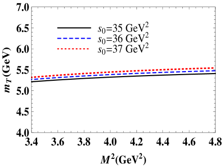
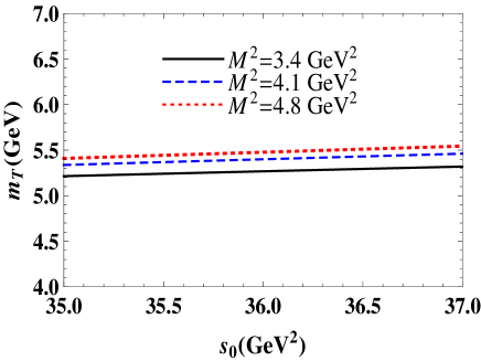
Figure 1: The mass of the tetraquark $T$ as a function of the Borel parameter $M^{2}$ at fixed $s_{0}$ (left panel) and as a function of the continuum threshold $s_{0}$ at fixed $M^{2}$ (right panel).

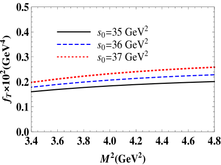
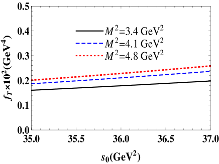
Figure 2: The same as in Fig. 1, but for the coupling $f_{T}$ of the state $T$.

Our calculations for the spectroscopic parameters of the tetraquark $T$ lead to the following results:

$$m_{T} = (5380~{}\pm 170)~{}\mathrm{MeV},$$

$$f_{T} = (2.1\pm 0.5)\times 10^{-3}\ \mathrm{GeV}^{4}.$$ (14)

The mass of the tetraquarks $T$ allows us to see whether this four-quark meson is strong-interaction stable or not. As we have emphasized above, $T$ contains the same quark species like the resonance $X(5568)$, but differs from it by an internal organization. The resonance $X(5568)$ with the content $su\overline{b}\overline{d}$ was originally studied in our work Agaev:2016mjb . It is a scalar particle, but has the heavy diquark-antidiquark structure. The mass of the resonance $X(5568)$ evaluated there

$$m_{X}=(5584~{}\pm 137)~{}\mathrm{MeV}$$ (15)

is higher than the mass of the tetraquark $T$; structures with a heavy diquark and a light antidiquark seem are more compact than ones composed of a pair of heavy diquark and antidiquark. The resonance $X(5568)$ is unstable against the strong interactions and decays to the conventional mesons $B_{s}^{0}\pi^{+}$. It is clear that $T$ cannot decay to such final states, but its quark content and quantum numbers does not forbid $S$-wave decays to $\overline{B^{0}}K^{-}/\overline{K^{0}}B^{-}$ mesons, thresholds of which $5774/5777~{}\mathrm{MeV}$ however, are above the mass $m_{T}$. Thresholds for $P$-wave decays of the scalar tetraquark $bs\overline{u}\overline{d}$ are higher than $m_{T}$ as well. The possible electromagnetic decay $T\rightarrow B^{-}K_{1}\gamma$ may be realized only if $m_{T}\geq 6552\ \mathrm{MeV}$, which is not the case. Therefore, transformation of the tetraquark $T$ to ordinary mesons runs only due to its weak decays.

III Semileptonic decays $Z_{bc}^{0}\rightarrow Te^{+}\nu_{e}$ and $Z_{bc}^{0}\rightarrow T\mu^{+}\nu_{\mu}$

In this section we explore the semileptonic decays $Z_{bc}^{0}\rightarrow Te^{+}\nu_{e}$ and $Z_{bc}^{0}\rightarrow T\mu^{+}\nu_{\mu}$ of the scalar four-quark meson $Z_{bc}^{0}$. The spectroscopic parameters of $Z_{bc}^{0}$ evaluated in Ref. Agaev:2018khe , as well as the mass and coupling of the final-state tetraquark $T$ , obtained in the previous section provide necessary information to calculate the differential rate and width of these decays.

The decay $Z_{bc}^{0}\rightarrow T\overline{l}\nu_{l}$ runs through the sequence of transformations $c\rightarrow W^{+}s$ and $W^{+}\rightarrow\overline{l}\nu_{l}$, and processes with $l=e$ and $\mu$ are kinematically allowed ones. At the tree level the transition $c\rightarrow s$ is described by the effective Hamiltonian

$$\mathcal{H}^{\mathrm{eff}}=\frac{G_{F}}{\sqrt{2}}V_{cs}\overline{s}\gamma_{\mu}(1-\gamma_{5})c\overline{l}\gamma^{\mu}(1-\gamma_{5})\nu_{l},$$ (16)

where $G_{F}$ is the Fermi coupling constant and $V_{cs}$ is the CKM matrix element. Sandwiching $\mathcal{H}^{\mathrm{eff}}$ between the initial and final tetraquarks, and factoring out the lepton fields we get the matrix element of the current

$$J_{\mu}^{\mathrm{tr}}=\overline{s}\gamma_{\mu}(1-\gamma_{5})c.$$ (17)

In terms of the weak form factors $G_{i}(q^{2})$ this matrix element has the form

$$\langle T(p^{\prime})|J_{\mu}^{\mathrm{tr}}|Z(p)\rangle=G_{1}(q^{2})P_{\mu}+G_{2}(q^{2})q_{\mu},$$ (18)

where $p$ and $p^{\prime}$ are the momenta of the tetraquarks $Z_{bc}^{0}$ and $T$, respectively. In Eq. (18) the form factors $G_{1}(q^{2})$ and $G_{2}(q^{2})$ parameterize the long-distance dynamics of the weak transition. Here we also use $P_{\mu}=p_{\mu}^{\prime}+p_{\mu}$ and $q_{\mu}=p_{\mu}-p_{\mu}^{\prime}$. The $q_{\mu}$ is the momentum transferred to the leptons, and evidently $q^{2}$ changes within the limits $m_{l}^{2}\leq q^{2}\leq(m_{Z}-m_{T})^{2}$, where $m_{l}$ is the mass of a lepton $l$.

To derive the sum rules for the form factors $G_{i}(q^{2}),i=1,2$ we begin from the three-point correlation function

$$\Pi_{\mu}(p,p^{\prime}) = i^{2}\int d^{4}xd^{4}ye^{i(p^{\prime}y-px)}$$ (19)

$$\times\langle 0|\mathcal{T}\{J(y)J_{\mu}^{\mathrm{tr}}(0)J^{Z\dagger}(x)\}|0\rangle,$$

where $J(y)$ and $J^{Z}(x)$ are the interpolating currents for the states $T$ and $Z_{bc}^{0}$, respectively. The current $J(y)$ has been defined above by Eq. (1): for $J^{Z}(x)$ we use the expression Agaev:2018khe

$$J^{Z}(x) = b_{a}^{T}(x)C\gamma_{5}c_{b}(x)\left[\overline{u}_{a}(x)\gamma_{5}C\overline{d}_{b}^{T}(x)\right.$$ (20)

$$\left.-\overline{u}_{b}(x)\gamma_{5}C\overline{d}_{a}^{T}(x)\right].$$

The current $J^{Z}(x)$ is composed of the $S$-wave diquark fields, has the antisymmetric color structure $[\overline{3}_{c}]_{bc}\otimes[3_{c}]_{\overline{u}\overline{d}}$ and describes the ground-state tetraquark $Z_{bc}^{0}$.

As usual, we express the correlation function $\Pi_{\mu}(p,p^{\prime})$ in terms of the spectroscopic parameters of the involved particles, and find the physical side of the sum rule $\Pi_{\mu}^{\mathrm{Phys}}(p,p^{\prime})$.  The function $\Pi_{\mu}^{\mathrm{Phys}}(p,p^{\prime})$ can be easily written down as

$$\Pi_{\mu}^{\mathrm{Phys}}(p,p^{\prime})=\frac{\langle 0|J|T(p^{\prime})\rangle\langle T(p^{\prime})|J_{\mu}^{\mathrm{tr}}|Z(p)\rangle}{(p^{2}-m_{Z}^{2})(p^{\prime 2}-m_{T}^{2})}$$

$$\times\langle Z(p)|J^{Z\dagger}|0\rangle+\ldots,$$ (21)

where we take explicitly into account contribution only of the ground-state particles, and denote by dots effects of the excited and continuum states.

The phenomenological side of the sum rules can be further simplified by rewriting the relevant matrix elements in terms of the tetraquark’s parameters, and employing for $\langle T(p^{\prime})|J_{\mu}^{\mathrm{tr}}|Z(p)\rangle$ its expression through the weak transition form factors $G_{i}(q^{2})$. To this end, we use Eq. (4) and the matrix element of the state $Z_{bc}^{0}$ defined by

$$\langle Z(p)|J^{Z\dagger}|0\rangle=f_{Z}m_{Z}.$$ (22)

Then it is not difficult to find that

$$\Pi_{\mu}^{\mathrm{Phys}}(p,p^{\prime}) = \frac{f_{T}m_{T}f_{Z}m_{Z}}{(p^{2}-m_{Z}^{2})(p^{\prime 2}-m_{T}^{2})}$$ (23)

$$\times\left[G_{1}(q^{2})P_{\mu}+G_{2}(q^{2})q_{\mu}\right].$$

We determine also $\Pi_{\mu}(p,p^{\prime})$ by employing the interpolating currents and quark propagators, which lead to its expression in terms of quark, gluon, and mixed vacuum condensates. In terms of the quark-gluon degrees of freedom $\Pi_{\mu}(p,p^{\prime})$ takes the form

$$\Pi_{\mu}^{\mathrm{OPE}}(p,p^{\prime})=i^{2}\int d^{4}xd^{4}ye^{i(p^{\prime}y-px)}\epsilon\widetilde{\epsilon}\mathrm{Tr}\left[\gamma_{\mu}(1-\gamma_{5})\right.$$

$$\left.\times S_{c}^{ib^{\prime}}(-x)\gamma_{5}\widetilde{S}_{b}^{ba^{\prime}}(y-x)\gamma_{5}S_{s}^{ci}(y)\right]\left\{\mathrm{Tr}\left[\gamma_{5}\widetilde{S}_{d}^{a^{\prime}e}(x-y)\right.\right.$$

$$\left.\left.\times\gamma_{5}S_{u}^{b^{\prime}d}(x-y)\right]-\mathrm{Tr}\left[\gamma_{5}\widetilde{S}_{d}^{b^{\prime}e}(x-y)\gamma_{5}S_{u}^{a^{\prime}d}(x-y)\right]\right\},$$

(24)

where $a^{\prime}$, $b^{\prime}$ and $i$ are the color indices of the currents $J^{Z}(x)$ and $J_{\mu}^{\mathrm{tr}}$, respectively.

We extract the sum rules for the form factors $G_{i}(q^{2})$ by equating the invariant amplitudes corresponding to the same Lorentz structures in $\Pi_{\mu}^{\mathrm{Phys}}(p,p^{\prime})$ and $\Pi_{\mu}^{\mathrm{OPE}}(p,p^{\prime})$. After that, we carry out the double Borel transformation over the variables $p^{\prime 2}$ and $p^{2}$ necessary to suppress contributions of the higher excited and continuum states, and finally carry out the continuum subtraction. These manipulations yield the sum rules

$$G_{i}(\mathbf{M}^{2},\ \mathbf{s}_{0},~{}q^{2})=\frac{1}{f_{T}m_{T}f_{Z}m_{Z}}\int_{(m_{b}+m_{c})^{2}}^{s_{0}}ds$$

$$\times\int_{\mathcal{M}^{2}}^{s_{0}^{\prime}}ds^{\prime}\rho_{i}(s,s^{\prime},q^{2})e^{(m_{Z}^{2}-s)/M_{1}^{2}}e^{(m_{T}^{2}-s^{\prime})/M_{2}^{2}}.$$ (25)

Here $\mathbf{M}^{2}=(M_{1}^{2},\ M_{2}^{2})$ and $\mathbf{s}_{0}=(s_{0},\ s_{0}^{\prime})$ are the Borel and continuum threshold parameters, respectively. It is worth noting that the set $(M_{1}^{2},s_{0})$ describes $Z_{bc}^{0}$, whereas $(M_{2}^{2},s_{0}^{\prime})$ corresponds to the $T$ tetraquark channel. The spectral densities $\rho_{i}(s,s^{\prime},q^{2})$ are calculated as the imaginary parts of the correlation function $\Pi_{\mu}^{\mathrm{OPE}}(p,p^{\prime})$ with dimension-five accuracy, and contain both the perturbative and nonperturbative contributions.

For numerical computations of $G_{i}(\mathbf{M}^{2},\ \mathbf{s}_{0},~{}q^{2})$ one needs to employ various parameters, values some of which are collected in Eq. (10). The mass and coupling of the tetraquark $Z_{bc}^{0}$ and $(M_{1}^{2},s_{0})$ are borrowed from Ref. Agaev:2018khe , whereas for $m_{T}$ and $f_{T}$, and $(M_{2}^{2},s_{0}^{\prime})$ we use results of the previous section.

To obtain the width of the decay $Z_{bc}^{0}\rightarrow T\overline{l}v_{l}$ we have to integrate the differential decay rate $d\Gamma/dq^{2}$ within the kinematical limits $m_{l}^{2}\leq q^{2}\leq(m_{Z}-m_{T})^{2}$, whereas the QCD sum rules lead to reliable results only for $m_{l}^{2}\leq q^{2}\leq 1.25$ $\mathrm{GeV}^{2}$. To cover all values of $q^{2}$ we replace the weak form factors by the functions $F_{i}(q^{2})$, which at accessible for the sum rule computations $q^{2}$ coincide with $G_{i}(q^{2})$, but can be extrapolated to the whole integration region.

In the present work for the fit functions we utilize the analytic expressions

$$F_{i}(q^{2})=f_{i}^{0}\exp\left[c_{1}^{i}\frac{q^{2}}{m_{Z}^{2}}+c_{2}^{i}\left(\frac{q^{2}}{m_{Z}^{2}}\right)^{2}\right].$$ (26)

Here, $f_{i}^{0},~{}c_{1}^{i}$ and $c_{2}^{i}$ are fitting parameters, values of which are presented below

$$f_{1}^{0} = 0.144,\ c_{1}^{1}=7.68,\ c_{2}^{1}=1505.10,$$

$$f_{2}^{0} = 3.282,\ c_{1}^{2}=7.69,\ c_{2}^{2}=1504.40.$$ (27)

In Fig. 3, as an example, we plot the sum rule predictions for the form factor $G_{1}(q^{2})$ and the fit function $F_{1}(q^{2})$ : It is seen that the fit function coincides well with the sum rule predictions in the region $m_{l}^{2}\leq q^{2}\leq 1.25$ $\mathrm{GeV}^{2}$.

The differential rate $d\Gamma/dq^{2}$ of the semileptonic decay $Z_{bc}^{0}\rightarrow T\overline{l}\nu_{l}$ is given by the formula

$$\frac{d\Gamma}{dq^{2}} = \frac{C_{F}^{2}|V_{cs}|^{2}}{64\pi^{3}m_{Z}^{3}}\lambda\left(m_{Z}^{2},m_{T}^{2},q^{2}\right)\left(\frac{q^{2}-m_{l}^{2}}{q^{2}}\right)^{2}\left\{(2q^{2}+m_{l}^{2})\left[|G_{1}(q^{2})|^{2}\left(\frac{q^{2}}{2}-m_{Z}^{2}-m_{T}^{2}\right)-|G_{2}(q^{2})|^{2}\frac{q^{2}}{2}\right.\right.$$ (28)

$$\left.+(m_{T}^{2}-m_{Z}^{2})\mathrm{\operatorname{Re}}\left[G_{1}(q^{2})G_{2}^{\ast}(q^{2})\right]\right]+\frac{q^{2}+m_{l}^{2}}{q^{2}}\left[|G_{1}(q^{2})|^{2}(m_{Z}^{2}-m_{T}^{2})^{2}+|G_{2}(q^{2})|^{2}q^{4}+2\mathrm{\operatorname{Re}}\left[G_{1}(q^{2})G_{2}^{\ast}(q^{2})\right]\right.$$

$$\left.\left.\times(m_{Z}^{2}-m_{T}^{2})q^{2}\right]\right\},$$

where

$$\lambda\left(m_{Z}^{2},m_{T}^{2},q^{2}\right)=\left[m_{Z}^{4}+m_{T}^{4}+q^{4}-2\left(m_{Z}^{2}m_{T}^{2}+m_{Z}^{2}q^{2}+m_{T}^{2}q^{2}\right)\right]^{1/2}.$$ (29)

To fulfil the numerical computations using Eq.(28) one also needs the Fermi coupling constant $G_{F}=1.16637\times 10^{-5}~{}\mathrm{GeV}^{-2}$ and CKM matrix element $|V_{cs}|=0.997\pm 0.017$. Obtained results for the width of semileptonic decays $Z_{bc}^{0}\rightarrow T\overline{l}\nu_{l}$ ($l=e,~{}\mu$) read

$$\Gamma\left(Z_{bc}^{0}\rightarrow Te^{+}\nu_{e}\right) = \left(1.19\pm 0.26\right)\times 10^{-11}\ \mathrm{MeV},$$

$$\Gamma\left(Z_{bc}^{0}\rightarrow T\mu^{+}\nu_{\mu}\right) = \left(1.18\pm 0.25\right)\times 10^{-11}\ \mathrm{MeV}.$$

These results are important part of the information to evaluate the full width and mean lifetime of the tetraquark $Z_{bc}^{0}$, and estimate branching ratios of its weak decay channels.

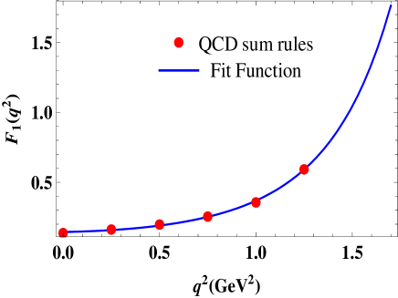
Figure 3: The sum rule predictions for the weak form factor $G_{1}(q^{2})$ and the fit function $F_{1}(q^{2})$.

IV Nonleptonic two-body decays $Z_{bc}^{0}\rightarrow T\pi^{+}$ and $Z_{bc}^{0}\rightarrow TK^{+}$

The nonleptonic two-body decays $Z_{bc}^{0}\rightarrow T\pi^{+}$ and $Z_{bc}^{0}\rightarrow TK^{+}$ of the tetraquark $Z_{bc}^{0}$ can be considered in the context of the QCD factorization approach, which allows us to calculate the amplitudes and widths of these processes. This method was successfully applied to study two-body weak decays of the conventional mesons Beneke:1999br ; Beneke:2000ry , and is used here to investigate two-body decays of the tetraquark $Z_{bc}^{0}$, when one of the final particles is an exotic meson.

At the quark level, the effective Hamiltonian for the decay $Z_{bc}^{0}\rightarrow T\pi^{+}$ is given by the expression

$$\widetilde{\mathcal{H}}^{\mathrm{eff}}=\frac{G_{F}}{\sqrt{2}}V_{cs}V_{ud}^{\ast}\left[c_{1}(\mu)Q_{1}+c_{2}(\mu)Q_{2}\right],$$ (31)

where

$$Q_{1} = \left(\overline{u}_{i}d_{i}\right)_{\mathrm{V-A}}\left(\overline{s}_{j}c_{j}\right)_{\mathrm{V-A}},$$

$$Q_{2} = \left(\overline{u}_{i}d_{j}\right)_{\mathrm{V-A}}\left(\overline{s}_{j}c_{i}\right)_{\mathrm{V-A}},$$ (32)

and $i$ , $j$ are the color indices. Here $c_{1}(\mu)$ and $c_{2}(\mu)$ are the short-distance Wilson coefficients evaluated at the scale $\mu$ at which the factorization is assumed to be correct. The shorthand notation $\left(\overline{q}_{1}q_{2}\right)_{\mathrm{V-A}}$ in Eq. (32) means

$$\left(\overline{q}_{1}q_{2}\right)_{\mathrm{V-A}}=\overline{q}_{1}\gamma_{\mu}(1-\gamma_{5})q_{2}.$$ (33)

The amplitude of this decay can be written down in the following factorized form

$$\mathcal{A} = \frac{G_{F}}{\sqrt{2}}V_{cs}V_{ud}^{\ast}a_{1}(\mu)\langle\pi^{+}(q)|\left(\overline{u}_{i}d_{i}\right)_{\mathrm{V-A}}|0\rangle$$ (34)

$$\times\langle T(p^{\prime})|\left(\overline{s}_{j}c_{j}\right)_{\mathrm{V-A}}|Z(p)\rangle,$$

where

$$a_{1}(\mu)=c_{1}(\mu)+\frac{1}{N_{c}}c_{2}(\mu),$$ (35)

with $N_{c}$ being the number of quark colors. The amplitude $\mathcal{A}$ corresponds to the process in which the pion $\pi^{+}$ is generated directly from the color-singlet current $\left(\overline{u}_{i}d_{i}\right)_{\mathrm{V-A}}$. The matrix element $\langle T(p^{\prime})|\left(\overline{s}_{j}c_{j}\right)_{\mathrm{V-A}}|Z(p)$ has been defined above in Eq. (18), whereas the matrix element of the pion in given by the expression

$$\langle\pi^{+}|\left(\overline{u}_{i}d_{i}\right)_{\mathrm{V-A}}|0\rangle=if_{\pi}q_{\mu}.$$ (36)

and is determined by its decay constant $f_{\pi}$.

Then, it is not difficult to see that $\mathcal{A}$ takes the form

$$\mathcal{A} = i\frac{G_{F}}{\sqrt{2}}f_{\pi}V_{cs}V_{ud}^{\ast}a_{1}(\mu)$$ (37)

$$\times\left[G_{1}(q^{2})Pq+G_{2}(q^{2})q^{2}\right].$$

The width of the decay $Z_{bc}^{0}\rightarrow T\pi^{+}$ is equal to:

$$\Gamma\left(Z_{bc}^{0}\rightarrow T\pi^{+}\right)=\frac{G_{F}^{2}f_{\pi}^{2}}{32\pi m_{Z}^{3}}|V_{cs}|^{2}|V_{ud}|^{2}a_{1}^{2}(\mu)$$

$$\times\lambda\left[|G_{1}(m_{\pi}^{2})|^{2}(m_{Z}^{2}-m_{T}^{2})^{2}+|G_{2}(m_{\pi}^{2})|^{2}m_{\pi}^{4}\right.$$

$$\left.+2\operatorname{Re}\left[G_{1}(m_{\pi}^{2})G_{2}^{\ast}(m_{\pi}^{2})\right](m_{Z}^{2}-m_{T}^{2})m_{\pi}^{2}\right],$$ (38)

where $\lambda=\lambda(m_{Z}^{2},m_{T}^{2},m_{\pi}^{2})$ is the function given by Eq. (29). The similar analysis is valid for the second decay $Z_{bc}^{0}\rightarrow TK^{+}$, as well: relevant formulas can by obtained by replacements $V_{ud}\rightarrow V_{us}$, $f_{\pi}\rightarrow f_{K}$, and $m_{\pi}\rightarrow m_{K}$.

Numerical computations can be carried out after fixing the spectroscopic parameters of the light mesons $\pi^{+}$ and $K^{+}$. In calculations we use $m_{\pi}=139.570\ \mathrm{MeV}$, $f_{\pi}=131\ \mathrm{MeV}$, and $m_{K}=\left(493.677\pm 0.016\right)\ \mathrm{MeV}$, $f_{K}=(155.72\pm 0.51)\ \mathrm{MeV}$, respectively. The weak form factors $G_{1}(q^{2})$ and $G_{2}(q^{2})$, which are main ingredients of $\Gamma\left(Z_{bc}^{0}\rightarrow T\pi^{+}(K^{+})\right)$, have been obtained in the previous section. For CKM matrix elements we use $|V_{ud}|=0.974$ and $|V_{us}|=0.224$. The Wilson coefficients at the factorization scale $\mu=m_{c}$ are borrowed from Ref. Colangelo:2001cv

$$c_{1}(m_{c})=1.263,\ c_{2}(m_{c})=-0.513.$$ (39)

For the decay $Z_{bc}^{0}\rightarrow T\pi^{+}$, our calculations lead to the result

$$\Gamma\left(Z_{bc}^{0}\rightarrow T\pi^{+}\right)=\left(7.05\pm 1.52\right)\times 10^{-12}\ \mathrm{MeV},$$

(40)

which is smaller than widths of the semileptonic decays, but nevertheless is comparable with them. For the second process $Z_{bc}^{0}\rightarrow TK^{+}$ we get

$$\Gamma\left(Z_{bc}^{0}\rightarrow TK^{+}\right)=\left(1.02\pm 0.21\right)\times 10^{-12}~{}\mathrm{MeV}.$$

(41)

It is not difficult to see that effect of this decay to formation of the full width of the tetraquark $Z_{bc}^{0}$ is very small. The partial widths of the nonleptonic two-body decays obtained in this section will be used below to find the full width of $Z_{bc}^{0}$.

V Analysis and concluding remarks

The partial widths of the dominant semileptonic and two nonleptonic decay modes of $Z_{bc}^{0}$ allow us to evaluate its full width and mean lifetime

$$\Gamma_{\mathrm{full}} = (3.18\pm 0.39)\times 10^{-11}~{}\mathrm{MeV},\$$

$$\tau = 2.07_{-0.23}^{+0.29}\times 10^{-11}~{}\mathrm{s}.$$ (42)

As is seen, the scalar tetraquark $Z_{bc}^{0}$ is narrower than the master particle $T_{bb;\overline{u}\overline{d}}^{-}$, and its mean lifetime $20.7_{-2.3}^{+2.9}~{}\mathrm{ps}$ is considerably longer that the same parameter for $T_{bb;\overline{u}\overline{d}}^{-}$.

The weak decays of $Z_{bc}^{0}$ occur via the following channels:

i) $Z_{bc}^{0}\rightarrow Te^{+}\nu_{e}$,

ii) $Z_{bc}^{0}\rightarrow T\mu^{+}\nu_{\mu}$,

iii) $Z_{bc}^{0}\rightarrow T\pi^{+}$,

and

iv) $Z_{bc}^{0}\rightarrow TK^{+}$.

All of them leads to appearance of the strong- and electromagnetic-interaction stable tetraquark $T\equiv T_{bs;\overline{u}\overline{d}}^{-}$ that at next stages of the process dissociates weakly. The branching ratio for production, for example, of the final state $Te^{+}\nu_{e}$ is given by

$$\mathcal{BR}(Z_{bc}^{0}\rightarrow Te^{+}\nu_{e})=\Gamma\left(Z_{bc}^{0}\rightarrow Te^{+}\nu_{e}\right)/\Gamma_{\mathrm{full}}.$$ (43)

It is not difficult to find that

$$\mathcal{BR}(Z_{bc}^{0} \rightarrow Te^{+}\nu_{e})\simeq 0.38,~{}\mathcal{BR}(\ Z_{bc}^{0}\rightarrow T\mu^{+}\nu_{\mu})\simeq 0.37$$

$$\mathcal{BR}(Z_{bc}^{0} \rightarrow T\pi^{+})\simeq 0.22,~{}\mathcal{BR}(\ Z_{bc}^{0}\rightarrow TK^{+})\simeq 0.03.$$

The weak decays of $T_{bb;\overline{u}\overline{d}}^{-}$ can be analyzed by the same way. The relevant semileptonic modes at the final state contain the tetraquark $T_{bs;\overline{u}\overline{d}}^{-}$ and two opposite sign leptons accompanying by corresponding neutrinos $e^{-}e^{+}\nu_{e}\overline{\nu}_{e}$, $e^{-}\mu^{+}\overline{\nu}_{e}\nu_{\mu}$, $e^{+}\mu^{-}\nu_{e}\overline{\nu}_{\mu}$, $\mu^{+}\mu^{-}\nu_{\mu}\overline{\nu}_{\mu}$, $\tau^{-}e^{+}\nu_{e}\overline{\nu}_{\tau}$ and $\tau^{-}\mu^{+}\overline{\nu}_{\tau}\nu_{\mu}$. Other decay channels are formed by the final states $Te^{-}\overline{\nu}_{e}\pi^{+}$, $Te^{-}\overline{\nu}_{e}K^{+}$,  $T\mu^{-}\overline{\nu}_{\mu}\pi^{+}$, $T\mu^{-}\overline{\nu}_{\mu}K^{+}$, $T\tau^{-}\overline{v}_{\tau}\pi^{+}$, and $T\tau^{-}\overline{v}_{\tau}K^{+}$. The branching ratios of these channels can be found using the fact, that $\mathcal{BR}(T_{bb;\overline{u}\overline{d}}^{-}\rightarrow Z_{bc}^{0}e^{-}\overline{\nu}_{e})\simeq\mathcal{BR}(T_{bb;\overline{u}\overline{d}}^{-}\rightarrow Z_{bc}^{0}\mu^{-}\overline{\nu}_{\mu})=0.37$ and $\mathcal{BR}(T_{bb;\overline{u}\overline{d}}^{-}\rightarrow Z_{bc}^{0}\tau^{-}\overline{v}_{\tau})=0.26$ (see, Ref. Agaev:2018khe ). For some of decay modes we get:

$$\mathcal{BR}(T_{bb;\overline{u}\overline{d}}^{-} \rightarrow Te^{-}e^{+}\nu_{e}\overline{\nu}_{e})\simeq 0.141,$$

$$\mathcal{BR}(T_{bb;\overline{u}\overline{d}}^{-} \rightarrow T\mu^{+}\mu^{-}\nu_{\mu}\overline{\nu}_{\mu})\simeq 0.137,$$

$$\mathcal{BR}(T_{bb;\overline{u}\overline{d}}^{-} \rightarrow T\tau^{-}e^{+}\nu_{e}\overline{\nu}_{\tau})\simeq 0.099,$$

$$\mathcal{BR}(T_{bb;\overline{u}\overline{d}}^{-} \rightarrow Te^{-}\overline{\nu}_{e}\pi^{+})\simeq 0.081,$$

$$\mathcal{BR}(T_{bb;\overline{u}\overline{d}}^{-} \rightarrow Te^{-}\overline{\nu}_{e}K^{+})\simeq 0.011.$$ (45)

We have explored the weak decays of the scalar tetraquark $Z_{bc}^{0}$ including its dominant semileptonic transformations to $Te^{+}\nu_{e}$ and $T\mu^{+}\nu_{\mu}$, as well as the two-body nonleptonic decays $Z_{bc}^{0}\rightarrow T\pi^{+}$ and $Z_{bc}^{0}\rightarrow TK^{+}$, and estimated branching ratios of these final states. Because $Z_{bc}^{0}$ is stable against strong and electromagnetic decays, weak modes are important for its experimental studies: in accordance with recent analysis the production rate of the tetraquarks with the heavy diquark $bc$ at the LHC would be higher by two order of magnitude than four-quark mesons with $bb$ Ali:2018xfq .

Another issue studied here is decays of the tetraquark $T_{bb;\overline{u}\overline{d}}^{-}$. We have analyzed its decay chains consisting of sequential weak transformations to final states with $T$ and evaluated their branching ratios. These calculations are important to fix processes, where the axial-vector tetraquark $T_{bb;\overline{u}\overline{d}}^{-}$ should be searched for.

The predictions for the width and lifetime of $Z_{bc}^{0}$, as well as for the branching ratios (LABEL:eq:BR2) and (45) should be considered as first results for these quantities obtained using dominant weak decays of $Z_{bc}^{0}$ and $T_{bb;\overline{u}\overline{d}}^{-}$. In fact, here we have taken into account only processes $Z_{bc}^{0}\rightarrow Te^{+}\nu_{e}$, $Z_{bc}^{0}\rightarrow T\mu^{+}\nu_{\mu}$, $Z_{bc}^{0}\rightarrow T\pi^{+}$ and $Z_{bc}^{0}\rightarrow TK^{+}$, but subdominant semileptonic decays of $Z_{bc}^{0}$ may correct these predictions. We have treated $T$ as a scalar particle, whereas $Z_{bc}^{0}$ can decay also to exotic mesons with another quantum numbers. By including into analysis these options one can open up new decay modes of $Z_{bc}^{0}$, and improve predictions for the branching ratios presented above. Finally, there are nonleptonic three-meson decay channels, effects of which on the full width and mean lifetime of $Z_{bc}^{0}$ maybe sizeable. In other words, nonleading semileptonic decays of $Z_{bc}^{0}$, its decays to a tetraquark $T$ with another quantum numbers, and to multimeson nonleptonic final states may improve and correct the picture described here. Detailed investigations of these problems, left beyond the scope of the present work, are necessary to gain more precise knowledge about properties of the exotic states $T_{bb;\bar{u}\bar{d}}^{-}$ and $Z_{bc}^{0}$.

.

References

(1) J. P. Ader, J. M. Richard and P. Taxil,
Phys. Rev. D 25, 2370 (1982).
(2) H. J. Lipkin,
Phys. Lett. B 172, 242 (1986).
(3) S. Zouzou, B. Silvestre-Brac, C. Gignoux and
J. M. Richard, Z. Phys. C 30, 457 (1986).
(4) J. Carlson, L. Heller and J. A. Tjon,
Phys. Rev. D 37, 744 (1988).
(5) S. Pepin, F. Stancu, M. Genovese and J. M. Richard,
Phys. Lett. B 393, 119 (1997).
(6) D. Janc and M. Rosina,
Few Body Syst. 35, 175 (2004)
(7) Y. Cui, X. L. Chen, W. Z. Deng and S. L. Zhu,
HEPNP 31, 7 (2007).
(8) J. Vijande, A. Valcarce and K. Tsushima,
Phys. Rev. D 74, 054018 (2006).
(9) D. Ebert, R. N. Faustov, V. O. Galkin and W. Lucha,
Phys. Rev. D 76, 114015 (2007).
(10) F. S. Navarra, M. Nielsen and S. H. Lee,
Phys. Lett. B 649, 166 (2007).
(11) M. L. Du, W. Chen, X. L. Chen and S. L. Zhu,
Phys. Rev. D 87, 014003 (2013).
(12) T. Hyodo, Y. R. Liu, M. Oka, K. Sudoh and S. Yasui,
Phys. Lett. B 721, 56 (2013).
(13) A. Esposito, M. Papinutto, A. Pilloni,
A. D. Polosa and N. Tantalo,
Phys. Rev. D 88, 054029 (2013).
(14) R. Aaij et al. [LHCb Collaboration],
Phys. Rev. Lett. 119, 112001 (2017).
(15) M. Karliner and J. L. Rosner,
Phys. Rev. Lett. 119, 202001 (2017).
(16) E. J. Eichten and C. Quigg,
Phys. Rev. Lett. 119, 202002 (2017).
(17) S. S. Agaev, K. Azizi, B. Barsbay and H. Sundu,
Phys. Rev. D 99, 033002 (2019).
(18) S. S. Agaev, K. Azizi and H. Sundu,
Phys. Rev. D 95, 034008 (2017).
(19) G.-Q. Feng, X.-H. Guo and B.-S. Zou,
arXiv:1309.7813 [hep-ph].
(20) W. Chen, T. G. Steele and S. L. Zhu,
Phys. Rev. D 89, 054037 (2014).
(21) A. Francis, R. J. Hudspith, R. Lewis and
K. Maltman,
arXiv:1810.10550 [hep-lat].
(22) T. F. Carames, J. Vijande and A. Valcarce,
arXiv:1812.08991 [hep-ph].
(23) A. Ali, Q. Qin and W. Wang,
Phys. Lett. B 785, 605 (2018).
(24) M. A. Shifman, A. I. Vainshtein and V. I. Zakharov,
Nucl. Phys. B 147, 385 (1979).
(25) M. A. Shifman, A. I. Vainshtein and V. I. Zakharov,
Nucl. Phys. B 147, 448 (1979).
(26) R. M. Albuquerque, J. M. Dias,
K. P. Khemchandani, A. Martinez Torres, F. S. Navarra, M. Nielsen and
C. M. Zanetti, arXiv:1812.08207 [hep-ph].
(27) S. S. Agaev, K. Azizi and H. Sundu,
Phys. Rev. D 93, 074024 (2016).
(28) R. L. Jaffe, Phys. Rept. 409, 1 (2005).
(29) H. Sundu, B. Barsbay, S. S. Agaev and K. Azizi,
Eur. Phys. J. A 54, 124 (2018).
(30) M. Beneke, G. Buchalla, M. Neubert and
C. T. Sachrajda, Phys. Rev. Lett. 83, 1914 (1999).
(31) M. Beneke, G. Buchalla, M. Neubert and
C. T. Sachrajda, Nucl. Phys. B 591, 313 (2000).
(32) P. Colangelo, and F. De Fazio, Phys. Lett. B
520, 78 (2001).