A set of $4d-3$ observables to determine any pure qudit state

Abstract

We present a tomographic method which requires only $4d-3$ measurement outcomes to reconstruct any pure quantum state of arbitrary dimension $d$. Using the proposed scheme we have experimentally reconstructed a large number of pure states of dimension $d=7$, obtaining a mean fidelity of $0.94$. Moreover, we performed numerical simulations of the reconstruction process, verifying the feasibility of the method for higher dimensions. In addition, the a priori assumption of purity can be certified within the same set of measurements, what represents an improvement with respect to other similar methods and contributes to answer the question of how many observables are needed to uniquely determine any pure state.

Quantum information processing is a field of research in constant growth since the last decades. It has been crucial both in the fundamental tests of quantum mechanics as well in the development of a vast number of technological applications Alber et al. (2003). A fundamental problem that transverse the entire field is that of determining the unknown state of a quantum system Paris and Řeháček (2004). In this regard, the process of reconstructing a general state of dimension $d$, known as quantum tomography, consists in finding its density matrix $\rho$, a positive semidefinite matrix with unit trace that fully describes the system. As the number of independent parameters that defines an arbitrary density matrix $\rho$ is $d^{2}-1$, typical quantum tomography schemes require a number of measurement outcomes that increases as $d^{2}$ James et al. (2001); Wootters and Fields (1989); Adamson and Steinberg (2010), leading to time consuming measurements and post processing, that can become prohibitive for high dimension systems Kaznady and James (2009); Moroder et al. (2012). Furthermore, several applications such as quantum key distribution Cerf et al. (2002); Dada et al. (2011); Mower et al. (2013); Zhong et al. (2015); Mirhosseini et al. (2015), quantum communication complexity problems Martínez et al. (2019) or fundamental tests of quantum mechanics Cañas et al. (2014); Vértesi et al. (2010), can be improved by using $d$-level quantum systems of dimension grater than two (qudits). Therefore, it is of great interest to develop alternative methods that employ fewer measurement settings.

A significantly reduction in the number of measurements is feasible if a priori information about the unknown state is taken into account in the tomographic process. For example, in the case of permutationally invariant states, a set of measurements that scales polynomially with the number of qubits $n$ ($d=2^{n}$) is enough to perform the reconstruction of the matrix $\rho$ Moroder et al. (2012); Schwemmer et al. (2014), instead of applying the habitual process with exponential growth. In the case of mixed states of $n$ qudits a reconstruction scheme which employs only local measurements can efficiently give an estimation of the state Baumgratz et al. (2013), provided they are well approximated by matrix product operators. For low-rank states, compressed sensing techniques allow the reconstruction of $\rho$ from a number of measurement outcomes of the order of $d(\log d)^{2}$ by measuring the expectation values of enough observables chosen at random Flammia et al. (2012); Gross (2011).

Special attention has been paid to the reconstruction of pure states. It has been shown Finkelstein (2004) that there exists a positive-operator-valued measure (POVM) which consists of $2d$ projectors from whose probability outcomes it is possible to distinguish almost all pure states, except for a set of measure zero; when all the pure states are included, the number of required measurement outcomes increases. In Ref. Wang and Shang (2018), Wang et al. have proven that a set of $4d-3$ fixed projectors are enough to reconstruct any pure qudit. Additionally, they showed that this number can be reduced to at most $3d-2$ in an adaptive scheme, where the results of a first measurement of the particular unknown state in the canonical base ($d$ projections) are used to choose the remaining projectors.

A highly desirable feature of a tomographic scheme that uses a priori information, is that it also allows to verify if the initial assumption about the unknown state is true Chen et al. (2013). In this regard, Goyeneche et al. Goyeneche et al. (2015) have proposed, and experimentally tested, an adaptive method that requires a set of five measurement bases to determine any pure qudit in arbitrary dimension, and additionally certify the assumption of purity without extra measurement outcomes. In addition, Carmelli et al. have constructed in Carmeli et al. (2016) a set of five fixed bases for the tomography of any pure state.

Recently Pears Stefano et al. (2017), we have reported a quantum tomography method to reconstruct any pure photonic spatial qudit of arbitrary dimension from a set of only $4d$ measurement outcomes, in case of a fixed measurement settings, or $4d-3$ when the procedure is performed in an adaptive way. In that work, the qudits were codified in the discretized transverse momentum of single photons (slit states) Neves et al. (2004). The proposed experimental setup exploited the spatial nature of the codification to set a Mach-Zehnder interferometer in the state-estimation stage. This interferometer is used to implement the three-step Phase Shifting Interferometry technique (PSI) Creath (1988), which is ideally suited to find the phase of a light wavefront. As the method allows to reconstruct the whole wavefront from the interference pattern, the $4d$ measurement outcomes can be obtained in parallel by means of an image detector, reducing the measurement settings to only four, independently of the dimension $d$ of the quantum system Pears Stefano et al. (2017). This measurement scheme is extremely efficient, and work properly for spatial qudits where it is straightforward to parallelize the measurements. However, still missing an experimental implementation of such tomographic method for more general encoding systems.

In this Letter we generalize that result to reconstruct any unknown pure qudit of arbitrary dimension $d$ from the outcome frequencies of $4d-3$ projectors, which do not depend on the physical representation of the state. While this amount of projectors represents approximately $d$ more measurement outcomes than reported in Ref. Wang and Shang (2018) for an adaptive scheme, our method allows us to certify the assumption of purity. Conversely, our method requires in the order of $d$ measurements less than the method reported in Ref. Carmeli et al. (2016), but at the expense of using adaptive measurements. Then, our scheme close the gap in the number of measurement between both kind of methods suggesting that, in order to have a fixed set of observables, the number of measurements has to be increase to $5d$. Instead of that, if the number of measurements is expected to be reduced to $\sim 3d$, the possibility of discriminate pure from mixed states is lost.

Let us to start by describing the reconstruction process scheme. Any pure quantum state of dimension $d$ can be expressed as

$$|\Psi\rangle=\sum_{k=0}^{d-1}c_{k}|k\rangle,$$ (1)

where the $c_{k}~{}^{\prime}s$ are complex coefficients and $|k\rangle$ denotes one of the $d$ states of some base of the Hilbert space, in particular the canonical base. These complex coefficients can be explicitly written as $c_{k}=|c_{k}|e^{i\varphi_{k}}$, being $\varphi_{k}$ a real number. For each element $|k\rangle$ of the canonical base such that $k=0,2,3,...,d-1$, we can define a set of $d$-dimensional states

$$|\Psi_{\ell}^{(k)}\rangle=\left(|0\rangle+e^{i\pi/2\times\left(\ell-1/2\right)}|k\rangle\right)/\sqrt{2},~{}\ \ \ \ \ \ \ \ell=1,2,3$$ (2)

from which $3d-3$ projectors $\hat{P}_{\ell}^{(k)}=|\Psi_{\ell}^{(k)}\rangle\langle\Psi_{\ell}^{(k)}|$ are obtained. The outcome probabilities of these projectors $p_{\ell}^{(k)}=\langle\Psi|\hat{P}_{\ell}^{(k)}|\Psi\rangle=|\langle\Psi_{\ell}^{(k)}|\Psi\rangle|^{2}$, i. e., the probabilities of measuring every state $|\Psi_{\ell}^{(k)}\rangle$ in the state $|\Psi\rangle$, are related to the coefficients $c_{k}~{}^{\prime}s$ by the set of $d-1$ equations

$$\sqrt{2}c_{0}c_{k}^{*}=\left(p_{1}^{(k)}-p_{2}^{(k)}\right)+i\left(p_{3}^{(k)}-p_{2}^{(k)}\right),$$ (3)

where, without loss of generality, we have define $c_{0}$ as real. Thus, with the knowledge of $c_{0}\equiv+\sqrt{p_{0}}$, which is obtained from the probability $|\langle 0|\Psi\rangle|^{2}=p_{0}$, the remaining $c_{k}$ are determined. These $3d-2$ measurement outcomes are sufficient for determining a generic pure state, with the exception of a set of measure zero, corresponding to those with a null value of $c_{0}$. This limitation can be overcome with the addition of a previous measurement of the unknown state onto the canonical base, from which we redefine the element $|0\rangle$ to satisfy the condition $|c_{0}|=\underset{k}{Max}\{|c_{k}|\}$. This leads to require determining the average values of $4d-3$ observables to completely solve the the pure-states reconstruction problem.

A remarkable feature of the method is that the same set of $4d-3$ measurement outcomes allows to verify the a priori assumption of purity. Following a similar argument to the one in Ref. Goyeneche et al. (2015), lets us consider a quantum state of dimension $d$ represented by the density matrix $\rho$. If the state is pure, there is an unitary matrix $U$ that diagonalizes $\rho$ such that $\rho=U\tilde{\rho}U^{\dagger}$, with $\tilde{\rho}_{kl}=1$ for $k=l=1$ and $0$ in any other case. Hence, it is easy to see that:

$$\rho~{}~{}\mathrm{is~{}pure}\Leftrightarrow|\rho_{k,l}|^{2}=|\rho_{k,k}||\rho_{l,l}|~{},~{}~{}\forall k,l=0,\ldots,d-1.$$ (4)

Additionally, being $\rho$ a Hermitian matrix it can be written as $\rho=AA^{\dagger}$ for some operator $A$. As a consequence, its elements can be expressed as $\rho_{k,l}=\langle\textbf{v}_{k},\textbf{v}_{l}\rangle$, where $\{\textbf{v}_{k}\}_{k=0}^{d-1}$ are the row vectors of $A$, and $\langle~{},~{}\rangle$ indicates the inner product. According to the Cauchy-Schwarz statement Eq. (4) holds iff $\textbf{v}_{k}$ and $\textbf{v}_{l}$ are linearly dependent, and therefore the state will be pure iff the rows of $A$ are all parallel. Finally, to validate the purity assumption is enough to verify the $d-1$ equations

$$|\rho_{0,k}|^{2}=|\rho_{0,0}||\rho_{k,k}|~{},~{}~{}k=1,\ldots,d-1,$$ (5)

which are hold iff every $\textbf{v}_{k}$ with $k=1,\ldots,d-1$ is parallel to $\textbf{v}_{0}$, and by transitivity, they are all parallel to each other. Physically, $|\rho_{0,k}|$ is the visibility of the two slits interference pattern, and in the context of the present tomographic scheme, it can be calculated as $\sqrt{\frac{\left(p_{1}^{(k)}-p_{2}^{(k)}\right)^{2}+\left(p_{2}^{(k)}-p_{3}^{(k)}\right)^{2}}{2}}$. Besides, the right-hand side of Eq. (5) is the product of the relative intensities of these two slits in the encoding state, which are readily evaluated from a measurement in the canonical base. It is worth to remember the close relationship between the set of projectors $\hat{P}_{\ell}^{(k)}$ and the method of three step PSI. The index $\ell$ in Eq. (2) is related to an increment in steps of $\pi/2$ of the phase difference between $|k\rangle$ and the reference state $|0\rangle$. For every $k$, these three projectors correspond to the interference between the object beam and the reference beam for phase differences of $\pi/2$, $\pi$ and $\pi/2$. In fact, it can be shown that Eq. (3) leads to $\varphi_{k}=\arctan\frac{p_{3}^{(k)}-p_{2}^{(k)}}{p_{1}^{(k)}-p_{2}^{(k)}},$ which is the explicit solution for the phases $\varphi_{k}$ in the PSI method Creath (1988).

To experimentally test the tomographic method in the context of projective measurements we have used the set-up schematically depicted in Figure 1.

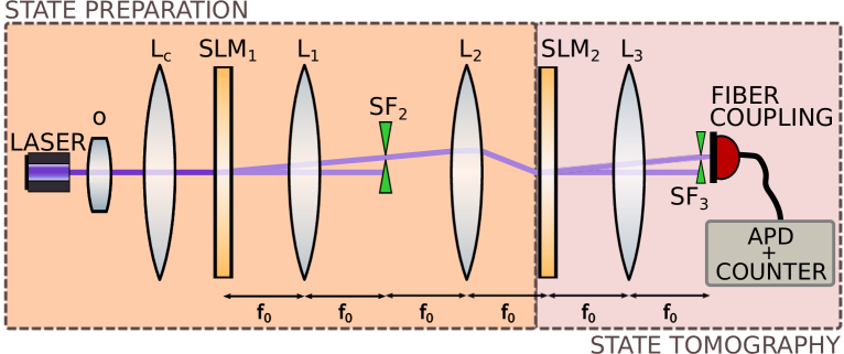
Figure 1: Experimental setup. The light source is a 405nm cw laser diode, attenuated down to the single photon level.
Ls: convergent lenses; SLMs: pure phase spatial light modulators; SFs: spatial filters. The detection in the centre of the interference pattern is performed with a fiber-coupled APD.

This setup can be divided in two modules, the first one is employed for the state preparation (SP) and the second one is used to perform the state tomography (ST). Let us start by describing the SP part that is basically a 4-f optical processor. The light source is a 405nm laser diode, attenuated to the single photon level. The beam is expanded by a microscope objective (O), spatially filtered ($\mathrm{SF}_{1}$) and then collimated by the $\mathrm{L}_{c}$ lens in such a way that onto the first Spatial Light Modulator (SLM), placed at the front focal plane of lens $\mathrm{L}_{1}$, a plane wave impinges with almost constant intensity distribution onto the region of interest (ROI). The SLM consists of a Sony liquid crystal television panel model LCX012BL that in combination with polarizers and wave plates, that provide the adequate state of polarization of light, allows a full phase modulation of the incident wavefront for the operating wavelength Marquez et al. (2001). By using the method described in the Ref. Solís-Prosser et al. (2013) it is possible to obtain at the back focal plane of lens $\mathrm{L}_{2}$ the complex amplitudes $c_{k}$ of an arbitrary slit state. Briefly, in this method each slit is represented by a phase grating. The absolute amplitude of each slit is controlled by means of the phase modulation of the grating as the diffraction efficiency depends on it. To encode this information we chose the first diffracted order, which is selected by ($\mathrm{SF}_{2}$). The argument of $c_{k}$ is obtained by adding an adequate uniform phase on the grating modulation. The ST is performed by using ($\mathrm{SLM}_{2}$) to provide the necessary phase modulation to encode the projector state by applying the same method used in the SP part. This second SLM is placed at the front focal plane of lens $\mathrm{L}_{3}$, so, after filtering the first diffracted order by means of $\mathrm{SF}_{3}$, the exact Fourier transform of the projected spatial qudit is obtained at the detector plane. The light distribution corresponds to the interference pattern projection between the prepared state and the selected projector state. The single photon count rate in the centre of the interference pattern is proportional to the probability of projection of the two states Lima et al. (2011). The detector module is a fiber-coupled avalanche photodiode (APD) photon counting module Perkin Elmer SPCM-AQRH-13-FC. The core aperture of the fiber ($\Phi=$ $62.5\,\,\mu\mathrm{m}$) acts as a pupil that selects the centre of the interference pattern.

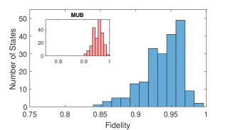
Figure 2: Histogram of the experimental reconstruction fidelity for 200 random states of dimension $d=7$. The mean fidelity is $\bar{F}=0.94$ and the standard deviation is $\sigma_{F}=0.03$. The inset shows the experimental reconstruction fidelity, for the same 200 states using the MUB method. The mean fidelity in this case is $\bar{F_{\mathrm{mub}}}=0.95$, and the standard deviation is $\sigma_{F_{\mathrm{mub}}}=0.03$. For this dimension our method only requires 25 projective measurements, while the MUB method requires 56.

We performed the reconstruction of a large number of pure states for dimension $d=7$. As a figure of merit of the reconstruction process we calculated the fidelity $F\equiv\mathrm{Tr}\left(\sqrt{\sqrt{\varrho}\rho\sqrt{\varrho}}\right)$ between the state intended to be prepared, $\varrho$, and the density matrix of the reconstructed state, $\rho$ Jozsa (1994). Fig. 2 shows an histogram of the reconstruction fidelity for 200 random pure states of dimension $d=7$. The mean fidelity is 0.94, with a standard deviation of 0.03. For comparison, we have also reconstructed the same set of states by means of a standard quantum tomography method using mutually unbiased bases (MUBs) Wootters and Fields (1989). In this case the mean fidelity is 0.95, with a standard deviation of 0.03. However, in our method only 25 projective measurements are necessary instead of the 56 used for implementing the MUBs method.

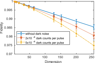
Figure 3: Simulated reconstruction fidelity as a function of the dimension. For each dimension, 2000 random states are reconstructed. The points represent the mean fidelity value, while the error bars are the standard deviation. Each curve corresponds to one simulation with a different average dark noise per pulse.

The feasibility of this technique was also tested numerically for several dimensions of the quantum system and different levels of experimental noise. To represent a realistic experimental implementation we assumed a pulsed attenuated laser as a source of weak coherent states, with a low mean number of photons per pulse $\mu$. We also include in our simulation a parameter $\lambda_{\mathrm{dc}}$ representing the mean dark counts per pulse caused by self triggering effects in the APD. As both, the photon emission process and the dark counts effect, are assumed to have a Poissonian statistic, the probability of detecting a photon after projecting $|\Psi\rangle$ onto the state $|\Psi_{\ell}^{(k)}\rangle$, within a given light pulse, is

$$\mathrm{Prob}\left(1\ \mathrm{count};\hat{P}_{\ell}^{(k)}\right)=1-\exp\left(-\mu p_{\ell}^{(k)}-\lambda_{\mathrm{dc}}\right).$$ (6)

If a fixed number of pulses $N$ is considered, the distribution for the detected counts is a Binomial distribution where the success probability is given by Eq. (6), and the mean number of counts in the state $|\Psi_{\ell}^{(k)}\rangle$ results

$$\macc@depth\char 1\relax\frozen@everymath{\macc@group}\macc@set@skewchar\macc@nested@a 111{n_{\ell}^{(k)}}=N\left\{1-\exp\left(-\mu p_{\ell}^{(k)}-\lambda_{\mathrm{dc}}\right)\right\}.$$ (7)

For small $\mu$ Eq. (7) is reduced to $\macc@depth\char 1\relax\frozen@everymath{\macc@group}\macc@set@skewchar\macc@nested@a 111{n_{\ell}^{(k)}}\approx N\mu p_{\ell}^{(k)}+N\lambda_{\mathrm{dc}},$ which makes straightforward to evaluate the state-reconstruction equation (Eq. (3)). Moreover, in our simulations we have used Eq. (7) to yield a closer estimation of the projection probabilities for every value of the parameters $\mu$ and $\lambda_{\mathrm{dc}}$.

In order to perform the numerical simulations we selected $\mu=0.18$ what results in $84\%$ of empty pulses and about $2\%$ of pulses with more than one photon, and a value $N=5\times 10^{4}$ to guarantee good statistics. Figure 3 shows the mean fidelity of the simulated results as a function of the state dimension for three levels of noise: without dark counts per pulse (solid line), $\lambda_{\mathrm{dc}}=2\times 10^{-4}$ (dotted line) and $\lambda_{\mathrm{dc}}=5\times 10^{-4}$ (dashed line) counts per pulse respectively. These last values are consistent with typical experimental situations, i. e., a pulse duration of the order of microseconds and an APD operating in the range of $100\mathrm{counts/sec}$. The error bar represents the standard deviation on the totality of states chosen randomly in the Hilbert space of dimension $d$. The fidelity values obtained from these simulations show that the proposed reconstruction method can be implemented in real high dimension systems.

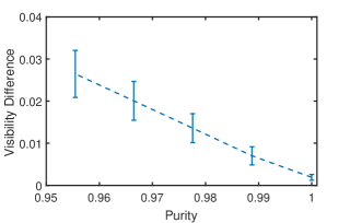
Figure 4: Visibility difference as a function of the degree of purity of the state. The curve is averaged over 2000 random states of dimension $d=8$. The points represent the average over states, while the error bars represent the standard deviation.

As the Eq. (5) only holds for pure states, the difference between both sides of the equality, i.e., the visibility difference between a pure quantum state compatible with the given measurement results and the unknown state that was actually measured, can be used as a discriminator between pure and mixed states. We tested this fact by numerically simulating the reconstruction with our tomographic scheme for random states of dimension $d=8$ affected by white noise. These states can be written as

$$\rho_{\mathrm{w}}(|\Psi\rangle,\lambda)=(1-\lambda)|\Psi\rangle\langle\Psi|+\lambda\mathbf{1}/d,$$ (8)

with $\lambda$ a real parameter related to the state purity by means of $\mathcal{P}(\rho_{\mathrm{w}})\equiv\mathcal{P}(\lambda)=\frac{d-1}{d}(\lambda-1)^{2}+\frac{1}{d}.$ Figure 4 shows the maximum difference between both size of Eqs. (5) as a function of the purity of the state $\rho_{\mathrm{w}}$, for a fixed value of $\lambda$. Each point in the curve represents the mean value of such a difference averaged over 2000 random states $|\Psi\rangle$. Hence, given a threshold of purity, this difference can be used to certify that the state surpass this value.

Summarizing, we have proposed a tomographic method to reconstruct any pure qudit state from only $4d-3$ projective measurement outcomes. Experimentally, we found good reconstruction fidelities for states of dimension $d=7$, comparable with the reconstruction fidelities obtained from the standard quantum tomography method using MUBs, but with the advantage of requiring a number of measurement outcomes that scale linearly with $d$, instead of $d^{2}$. Furthermore, we have shown through simulations that our scheme works properly in higher dimension systems, and it is suitable to distinguishing between pure and mixed states.