Rejoinder:
“Gene Hunting with Hidden Markov Model Knockoffs”

Abstract

In this paper we deepen and enlarge the reflection on the possible advantages of a knockoff approach to genome wide association studies (Sesia et al., 2018), starting from the discussions in Bottolo & Richardson (2019); Jewell & Witten (2019); Rosenblatt et al. (2019) and Marchini (2019). The discussants bring up a number of important points, either related to the knockoffs methodology in general, or to its specific application to genetic studies. In the following we offer some clarifications, mention relevant recent developments and highlight some of the still open problems.

1 Conditional vs. marginal hypotheses

The model-X framework of knockoffs (Candès et al., 2018) addresses a general multiple testing problem in which the $j$th null hypothesis states that the response $Y$ is independent of the explanatory variable $X_{j}$ conditional on all other predictors $X_{-j}$. In the very special case where the joint distribution of $X$ and $Y$ is multivariate Gaussian, this is equivalent to testing for the presence of conditional or partial correlations (Rosenblatt et al., 2019). In general, the non-null variables in the model-X framework are those belonging to the Markov blanket of $X$ on $Y$ (Candès et al., 2018).

There is little sense in arguing that, generally speaking, conditional or marginal hypotheses are the “right ones” to test: the choice between these two approaches will clearly depend on the problem at hand. For example, if $Y$ describes the cancer status of a tissue sample, and each $X_{j}$ the expression level of gene $j$, one might be interested in testing the hypotheses that $Y\mathchoice{\mathrel{\hbox to0.0pt{$\displaystyle\perp$\hss}\mkern 2.0mu{\displaystyle\perp}}}{\mathrel{\hbox to0.0pt{$\textstyle\perp$\hss}\mkern 2.0mu{\textstyle\perp}}}{\mathrel{\hbox to0.0pt{$\scriptstyle\perp$\hss}\mkern 2.0mu{\scriptstyle\perp}}}{\mathrel{\hbox to0.0pt{$\scriptscriptstyle\perp$\hss}\mkern 2.0mu{\scriptscriptstyle\perp}}}X_{j}$. The rejections of these null hypotheses would describe all genes whose expression level changes with cancer status. Whenever we think of relating a response $Y$ with a linear (or generalized linear) model in term of $X$, and test the hypotheses that the regression coefficients vanish, we are testing hypotheses that are of a conditional flavor (these hypotheses correspond exactly to the conditional ones in the case where the response follows a generalized linear model, see Candès et al. (2018)).

In a genome-wide association study, we find ourselves precisely in a situation of the latter type. The traits of interest are polygenic—they are influenced by the contribution of many genetic variants—and the models most commonly used by the scientific community are either linear or log-linear. Testing conditional hypotheses corresponds to trying to identify those genetic variants whose coefficients are nonzero in these models. As we pointed out in our paper, the literature has attempted to apply multivariate models since the very beginning; see for example Hoggart et al. (2008). While the scientific interest of the conditional hypotheses was never in question, the genetic community encountered a number of challenges in the application of multivariate methods that only recently we have begun to be able to address. A fundamental difficulty has been the inability to couple the findings of procedures such as the Lasso with precise reproducibility guarantees: in order to be able to associate a p-value to each of the genetic variants in the study, researchers resorted to marginal analysis. The knockoffs approach, by guaranteeing control of the false discovery rate over the selected variants, bypasses this difficulty and therefore opens the possibility of analyzing the data with those models that geneticists always thought provided a more accurate description of reality.

Rather than repeating ourselves, we would like to take the occasion to augment the discussion of this topic with some additional references. Firstly, let us point out that, as underscored by Marchini (2019), the standard methods of analysis of genome-wide association data already depart from an entirely marginal framework. By relying on linear mixed models (Zhang et al., 2010; Kang et al., 2010) with a covariance matrix estimated from the entire genotype data, geneticists effectively try to estimate the contribution of a specific variant $X_{j}$ in addition to that of the rest of the genome $X_{-j}.$ While this approach has proven a step forward, it still suffers from some important limitations: for example, it relies on fairly restrictive distributional assumptions, and requires the researcher to postulate a different model relating the phenotype $Y$ to the genotype $X$ for every variable that is analyzed. Possibly one of its most important limits is that it is unable to resolve the contribution of multiple variants in linkage disequilibrium—a topic that we shall discuss in greater depth later.

Secondly, we would like to refer the reader to two recent contributions (Buzdugan et al., 2016; Klasen et al., 2016) to the literature of genome-wide association studies going in a direction similar to ours; that is to say, enabling a multivariate analysis with some reproducibility guarantees. While these authors attempt to control the family-wise error rate, Buzdugan et al. (2016) in particular has interesting remarks on the conditional versus marginal hypotheses: they observe how, under appropriate assumptions, if “the coefficient [for the single nucleotide polymorphism (SNP) $j$] in the multivariate linear regression is different from zero, […] there exists a non-zero direct causal effect from SNP $j$ to the phenotype $Y$. This statement is not true with marginal associations (i.e. if SNP $j$ is only marginally associated with $Y$) since adjusting for all other SNPs (different from SNP $j$) is crucial for causal statements.” Since the ultimate scientific goal is to identify causal variants (Edwards et al., 2013; Visscher et al., 2017), this is a strong argument in favor of conditional hypotheses.

Finally, we want to underscore another sense in which marginal hypotheses are becoming less interesting in genome-wide association studies. As sample sizes $n$ increase, it has become apparent that polygenic traits are indeed influenced by a very large number of genetic variants (Boyle et al., 2017). Coupling this with the presence of linkage disequilibrium and the fact that large $n$ allows one to detect even small departures from independence, one realizes that, soon enough, we will be in the position to reject the marginal null $Y\mathchoice{\mathrel{\hbox to0.0pt{$\displaystyle\perp$\hss}\mkern 2.0mu{\displaystyle\perp}}}{\mathrel{\hbox to0.0pt{$\textstyle\perp$\hss}\mkern 2.0mu{\textstyle\perp}}}{\mathrel{\hbox to0.0pt{$\scriptstyle\perp$\hss}\mkern 2.0mu{\scriptstyle\perp}}}{\mathrel{\hbox to0.0pt{$\scriptscriptstyle\perp$\hss}\mkern 2.0mu{\scriptscriptstyle\perp}}}X_{j}$ for every $X_{j}$ in the genome, an utterly uninteresting result.

2 False discovery rate vs. family-wise error rate

Even though the family-wise error rate is still the most commonly used measure of type-I errors in genome-wide association studies (Rosenblatt et al., 2019), we feel quite strongly that the false discovery rate is arguably more appropriate. As modern studies of complex traits often lead to the discovery of several hundreds of loci (Visscher et al., 2017; Boyle et al., 2017), it seems excessive to worry about the probability of reporting a single false finding, especially when large leaps of faith are involved in the traditional postulation of the null hypotheses and in the assumptions of the linear models. The statistical genetics community has already widely accepted the concept of false discovery rate for the analysis of gene expression and other genomic measurements (Battle et al., 2017). It is more plausible that its adoption in genome-wide association studies has been hindered by the methodological difficulties arising from the correlations among the variants, rather than any fundamental objections to its principle. Therefore, as new statistical methods are developed, we expect that the use of the false discovery rate in genome-wide association studies will keep on expanding.

3 The resolution of conditional testing

In a genome-wide association study, each explanatory variable $X_{j}$ can naturally be chosen to represent a single nucleotide polymorphism, so that feature selection will be performed at the highest possible resolution allowed by the genotyped data. However, unless the signals are sufficiently strong, conditional testing may be a hopeless task and different hypotheses should be analyzed instead. For example, if $X_{1}$ and $X_{2}$ are nearly identical within the collected sample, it may be wiser to ask whether $Y\rotatebox[origin={c}]{90.0}{$\models$}(X_{1},X_{2})\mid X_{-\{1,2\}}$ rather than $Y\rotatebox[origin={c}]{90.0}{$\models$}X_{1}\mid X_{2},X_{-\{1,2\}}$ and $Y\rotatebox[origin={c}]{90.0}{$\models$}X_{2}\mid X_{1},X_{-\{1,2\}}$. Consequently, if knockoffs are applied to the individual hypotheses, $\tilde{X}_{1}$ and $\tilde{X}_{2}$ will certainly almost be equal to $X_{1}$ and $X_{2}$, and thus powerless (Rosenblatt et al., 2019). It is important to underline that this is not a limitation of our method. Instead, it is an inevitable reflection of the fundamental undecidability of the question that was asked, as conditional testing may only be performed at the resolution allowed by the data.

The solution adopted in our paper is that suggested in Candès et al. (2018): the variants are grouped based on their empirical correlations and knockoffs are only constructed for a set of promising prototypes identified through a suitable data carving scheme. Even though the choice of a resolution may be somewhat arbitrary in our paper, our methods can be easily applied with different values of the clumping correlation threshold. It is left to future research to determine whether an optimal choice exists, and how to combine the results obtained at different resolutions. As correctly pointed out in Jewell & Witten (2019), our approach formally amounts to asking whether $Y\rotatebox[origin={c}]{90.0}{$\models$}X^{*}_{j}\mid X^{*}_{-j}$, where $X^{*}_{j}$ indicates the prototype for the $j$th group.

Alternatively, one could directly test group-wise hypotheses of the type $Y\rotatebox[origin={c}]{90.0}{$\models$}(X_{1},X_{2})\mid X_{-\{1,2\}}$ by extending the notion of group knockoffs (Dai & Barber, 2016; Katsevich & Sabatti, 2017) to our methods. This approach arguably offers a more elegant interpretation as it completely avoids the pruning of any markers (Marchini, 2019), at some additional computational cost. For this purpose, we have already developed new efficient algorithms that will soon be presented as part of our follow-up work.

To put this in the context of the genetics literature, we note how the standard analysis of genome-wide association studies allows only the identification of loci that are (marginally) associated with the trait of interest, without discriminating between the many variants that are present at these loci. To increase the resolution of the findings, one resorts to what are known as “fine-mapping” methods (Hormozdiari et al., 2014; Spain & Barrett, 2015). These invariably rely on a multivariate model, and are also faced with the impossibility of resolving the signal beyond the level of information present in the data. For example, Hormozdiari et al. (2014) output a “causal set” of variants that is guaranteed to contain the truly causal ones, but will also include others, practically indistinguishable from these. An interesting feature of the knockoff-based approach to genome-wide association studies is that, effectively, it performs simultaneously locus identification and fine mapping.

4 Confounders

The confounding effect of an inhomogeneous population is a major source of concern in the marginal analysis of genome-wide association studies (Pritchard et al., 2000) and it is not surprising that the discussants bring this up (Marchini, 2019; Bottolo & Richardson, 2019). Because we do not expect the wide readership to be familiar with this issue, it is best to explain it in a few lines through a stylized example. Imagine that the statistician has available genotypes of individuals blindly sampled from the European and African populations, which have substantially different diets. Suppose further that our statistician is interested in the genetic determinants of blood lipid levels, which are also influenced by dietary intakes, and hence have a different mean level in the European and African population. Then all the variants $X_{j}$ which differ in frequency across the two populations (and there are many) will show a strong association with the response $Y$ and may get picked up. However, they may have no direct genetic link to blood lipids. Rather, a strong signal may be observed simply because the value of a marker is correlated to the population an individual belongs to, and different populations have different diets, and that diets influence blood lipid levels.

As recognized before (Klasen et al., 2016), conditional testing already implicitly accounts for any population structure. To quote from Klasen et al. (2016), “testing of markers with a high-dimensional variable selection procedure, which can account for the correlations between the markers, does not require any population structure correction at all.” This is simply because we are asking whether a particular variant $X_{j}$ provides information about the phenotype in addition to anything that can already be inferred from the value $X_{-j}$ of all the other hundreds of thousands of variables. Conditioning on $X_{-j}$ implies conditioning on the different ancestries of the individuals. To return to our example, if we get to see hundreds of thousands of genetic variants about an individual, then we already know which population this individual belongs to. In our analysis of the Northern Finland 1966 Birth Cohort study, the first 5 principal components of the genotype matrix are therefore included mainly to increase power.

The real issue here concerns the validity of the sampling mechanism. As observed in Bottolo & Richardson (2019), the hidden Markov model of Scheet & Stephens (2006) is better suited to describe populations that are homogeneous and unrelated, or that contain known patterns. If the structure of the sub-populations is unknown, more complex models (Falush et al., 2003; Delaneau et al., 2012; O’Connell et al., 2014, 2016) should be used to generate knockoffs. Since the modeling of inhomogeneous populations typically relies on more refined hidden Markov models, we can say in response to Bottolo & Richardson (2019) that the extension of our work is, at least conceptually, rather straightforward. This merely involves novel computational challenges that will be addressed in future work. Meanwhile, our current approach can be further justified by observing that knockoffs tend to be quite robust to some degree of model misspecification (Candès et al., 2018; Barber et al., 2018; Romano et al., 2018).

5 Case-control studies

Marchini (2019) asks about the impact of the artificial inflation in the frequency of the haplotypes surrounding the causal variants in case-control studies, and we pause to discuss this carefully. There are two populations we may want to think about: a prospective population $G_{XY}$ of individuals obeying certain characteristics; for instance, all adult males living in the UK; and a retrospective population $F_{XY}$ in which, to quote from Marchini, cases are usually more prevalent. In the retrospective population, the proportion of cases versus controls takes on an arbitrary value, which is typically higher than that in the prospective population. Formally, the relationship between the prospective and retrospective populations is as follows:

$$G_{X|Y}=F_{X|Y},\quad G_{Y}\neq F_{Y}.$$

The equality follows directly from the assumption that cases and controls in the study are randomly sampled from the prospective population of diseased and healthy individuals. The inequality is due to the fact that the proportions of cases typically differ. Consequently, the marginals are different as well, i.e., $G_{X}\neq F_{X}$.

In our work, we get independent samples from the retrospective population $F_{XY}$. Thus, as long as the hidden Markov model provides a good approximation for the marginal $F_{X}$, the method applies and the inference is valid. Since we estimate $F_{X}$ by relying on the genotypes of the cases and controls contained in our sample, we control the false discovery rate for testing $Y\mathchoice{\mathrel{\hbox to0.0pt{$\displaystyle\perp$\hss}\mkern 2.0mu{\displaystyle\perp}}}{\mathrel{\hbox to0.0pt{$\textstyle\perp$\hss}\mkern 2.0mu{\textstyle\perp}}}{\mathrel{\hbox to0.0pt{$\scriptstyle\perp$\hss}\mkern 2.0mu{\scriptstyle\perp}}}{\mathrel{\hbox to0.0pt{$\scriptscriptstyle\perp$\hss}\mkern 2.0mu{\scriptscriptstyle\perp}}}X_{j}|X_{-j}$ whenever $(X,Y)\sim F$. Although we do not prove this here, the definition of a null does not change whether $(X,Y)\sim G$ or $(X,Y)\sim F$ (we can loosely say that the definition of conditional independence does not depend on the distribution of the covariates). We believe this answers Marchini’s comment on type-1 error control.

There is a broader issue of interest as well. To be sure, we often claim that one attractive feature of the knockoffs approach is that we may want to use lots of unlabeled data to ‘learn’ the distribution of the covariates $X$. If this were the case, we would learn $G_{X}$, not $F_{X}$! We would then construct features that are exchangeable when $X\sim G_{X}$, perhaps not when $X\sim F_{X}$. What is the implication of this? A cool result is that despite this apparent mismatch, knockoffs constructed in this way provide valid inference as well when $X\sim F_{X}$! This fact will be rigorously established in a future publication. Our intent here is merely to explain that our approach allows considerable flexibility in the way we construct knockoff variables in case-control studies.

Marchini (2019) also asks about power. In light of our discussion, we may ask whether we should build knockoffs based upon $G_{X}$ or upon $F_{X}$ as to maximize power. This is an interesting but delicate question, which requires more analysis than we can possibly offer here.

6 What makes good negative control variables?

The idea to use pseudo-variables to guide the selection of important features is not new and goes back at least to Miller (1984), as remarked in Barber & Candès (2015). Having said this, there is a profound distinction between a vague program and an operational procedure that achieves clearly stated goals. This is best explained by focusing our remarks on the work of Wu et al. (2007), which is brought up by Rosenblatt et al. (2019), and on permutation techniques discussed in Bottolo & Richardson (2019).

Wu et al. (2007) state that ideal pseudo or phony variables should obey two properties recalled in Rosenblatt et al. (2019): “(A1) real unimportant variables and phony unimportant variables have the same probability of being selected on average”, and “(A2) real important variables have the same probability of being selected whether or not phony variables are present”. This is a wishful list that their paper does not show how to implement. In contrast, the knockoffs framework gives us (1) some precise rules for constructing synthetic features which can be safely used as negative controls and (2) a concrete selection procedure—a filter—which sifts through variable and knockoff scores computed via any method the statistician suspects to be powerful while rigorously controlling the false discovery rate (Barber & Candès, 2015); this filter is unlike anything we have seen in the literature. We expand on these two novelties below.

Knockoff variables are entirely different from existing pseudo-variables, including variables obtained by permutations, and we make this clear through the simplest possible example. Imagine we have $n$ i.i.d. samples $(X_{1}^{(i)},X_{2}^{(i)},Y^{(i)})$, $i=1,\ldots,n$, drawn from a population in which

$$(X_{1},X_{2})\sim\mathcal{N}(0,\Sigma)\quad\text{and}\quad Y|X_{1},X_{2}\sim\mathcal{N}(X_{1},1),$$

so that the first variable belongs to the linear model while the second does not. We assume that $X_{1}$ and $X_{2}$ have unit variance and that $\operatorname{corr}(X_{1},X_{2})=1/2$. By definition, knockoff variables obey $(\tilde{X}_{1},\tilde{X}_{2})\stackrel{{\scriptstyle\mathrm{d}}}{{=}}({X}_{1},\tilde{X}_{2})\stackrel{{\scriptstyle\mathrm{d}}}{{=}}(X_{1},X_{2})$, so that a knockoff feature correlates with a true feature in exactly the same way as a pair of true features; $\operatorname{corr}(X_{1},\tilde{X}_{2})=1/2$. How do the four pseudo-variable proposals of Wu et al. (2007) compare? In the first case, the pseudo variables $X_{1}^{*}$ and $X_{2}^{*}$ are independent standard normal and independent of anything else (the proposal would be the same if the covariates are not Gaussian as long as each marginal has mean zero and variance one). Clearly, $(X_{1}^{*},X_{2}^{*})$ is not at all distributed as $(X_{1},X_{2})$ and, moreover, $\operatorname{corr}(X_{1},X^{*}_{2})=0$.

In the second proposal, the pseudo-variables $(X_{1}^{*},X_{2}^{*})$ are obtained by applying a random permutation, see also Bottolo & Richardson (2019): concretely, the pseudo-variables for the $i$th observation are $\{(X_{1}^{(\pi(i))},X_{2}^{(\pi(i))})\}$, where $\pi$ is a random permutation from $\{1,\ldots,n\}$. By construction, we now have $(X_{1}^{*},X_{2}^{*})\stackrel{{\scriptstyle\mathrm{d}}}{{=}}(X_{1},X_{2})$. However, a simple calculation shows that whereas

$$\operatorname{corr}(X_{1},\tilde{X}_{2})=\frac{1}{2},\quad\operatorname{corr}(X_{1},X_{2}^{*})=\frac{1}{2n}.$$

In the limit of large samples, the correlation between $X_{1}$ and $X_{2}^{*}$ vanishes. So it is, once again, completely different. The remaining proposals in Wu et al. (2007) are refinements of the first two and operate by projecting the pseudo variables above onto the orthogonal complement of the space spanned by the original covariates.

Consider now what happens when we compute statistics for testing whether variables are in the model or not. Here, the sample correlation between $X_{2}$ and $Y$ has mean $1/2$ whereas that between $X_{2}^{*}$ and $Y$ vanishes (it is equal to $0.5/n$). Hence, the permutation $X_{2}^{*}$ cannot serve in any way as a negative control. To serve as a negative control, a phony variable needs to have the same explanatory power than the null variable being tested; colloquially, we might say that it needs to have the same $R^{2}$. A phony variable generated by a random permutation, however, is essentially independent of the response and has, therefore, no explanatory power whatsoever. These facts also apply to the forward selection method of Wu et al. (2007) as it is easy to imagine examples in which true nulls have a much higher chance of being selected than permuted features. In summary, permutation methods may be useful to test the existence of any relationship between a response and a family of covariates but they generally cannot be used to provide any finer-grained information (J. DiCiccio & Romano, 2016). It is, therefore, impossible to understand how the insights of Wu et al. (2007) “will later be formalized by knockoffs” as suggested by Rosenblatt et al. (2019).

A slightly more sophisticated example of the same principle is shown in the numerical experiment of Figure 1. Here, the performance of knockoffs is compared with that of permuted variables and independent Gaussian pseudo features, and the results provide a striking visual representation of why such phony variables cannot be used for calibration.

We turn to the second novelty. We live in an age where researchers have powerful and extremely complex data fitting strategies right at their fingertips; think of deep learning methods, sophisticated Bayesian computations, or a combination thereof. Knockoffs are designed to work with any feature-importance measures the statistician would like to use—not just the time of entry in a forward selection algorithm.

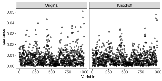
(a) Knockoffs can be safely used as negative controls because they are as likely to be selected as the unimportant original variables.

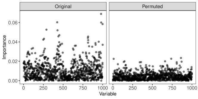
(b) Permuted variables cannot be used as negative controls because they are less likely to be selected than the unimportant original variables.

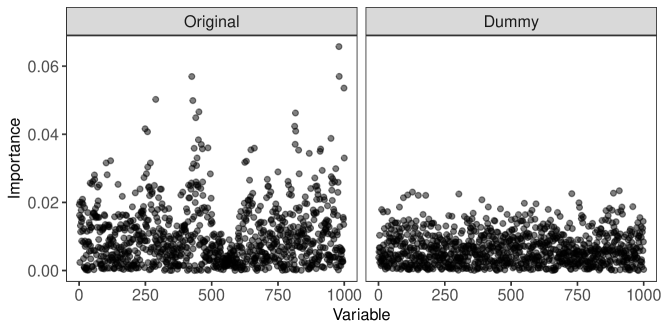
(c) White-noise dummy variables cannot be used as negative controls because they are less likely to be selected than the unimportant original variables.

Figure 1: Measures of feature importance computed with ridge regression on $n=1000$ independent realizations of $p=1000$ variables sampled from a hidden Markov model and augmented with different types of artificial covariates. The response is simulated from a linear model with 60 nonzero coefficients. The 60 truly important variables, i.e., those whose coefficients in the linear model are nonzero, are not shown.

7 Modeling the distribution of the explanatory variables

Generating valid knockoffs requires in principle perfect knowledge of the distribution $F_{X}$ of the explanatory variables. Fortunately, this goal is not unrealistic and a good degree of approximation can be achieved in practice for genome-wide association studies by leveraging the large amounts of available data and the prior knowledge encoded in the hidden Markov models of genetic variation (Li & Stephens, 2003). It is however natural to wonder about the behaviour of knockoffs under model misspecification in practice. The numerical results in Figure 2 of Jewell & Witten (2019) are consistent with our experience that knockoffs are typically quite robust. In fact, requiring that the joint distribution of $\tilde{X}$ and $X$ be exchangeable in the sense of Candès et al. (2018) is much stronger than asking for false discovery rate control at a nominal level for a specific choice of importance statistics. However, concrete examples can be found where an incorrect sampling mechanism leads to an inflation of the type-I errors (Romano et al., 2018).

For hidden Markov models, the approximate knockoffs of Candès et al. (2018) based on the Gaussian assumption are not rigorously guaranteed to control the false discovery rate and they are often less powerful than our exact construction. In order to show this point with an example, we have replicated the experiment of Figure 1 in Jewell & Witten (2019), with a small technical modification, as shown in Figures 2 and 3. Since the empirical covariance matrix of $X$ is almost singular in this simulation, Gaussian knockoffs based on the second-order approximation in Candès et al. (2018) have no power. The reason why our results in Figure 2 are different is that the empirical covariance matrix was shrunk in Jewell & Witten (2019), in the attempt to generate non-trivial Gaussian knockoffs. On the other hand, our algorithm provided with knowledge of the hidden Markov model structure can generate powerful knockoffs without violating exchangeability.

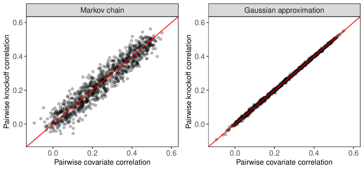
Figure 2: Simulation with $p=1000$ covariates distributed as a Markov chain and exact knockoffs generated using the approach in Sesia et al. (2018), as well as approximate Gaussian knockoffs obtained by applying the method of Candès et al. (2018). The experiment is the same as that of Figure 1 in Jewell & Witten (2019), although the covariance matrix for the Gaussian knockoffs is estimated differently. The figure shows the pairwise correlations among the covariates, $\text{Cor}(X_{j},X_{j-1})$, versus the pairwise correlations among the knockoffs, $\text{Cor}(\tilde{X}_{j},\tilde{X}_{j-1})$, for $j\in\{2,\ldots,p\}$. Left: exact knockoffs for the Markov chain; right: approximate Gaussian knockoffs. Both knockoff constructions generate synthetic features whose second moments are exchangeable with the original variables.

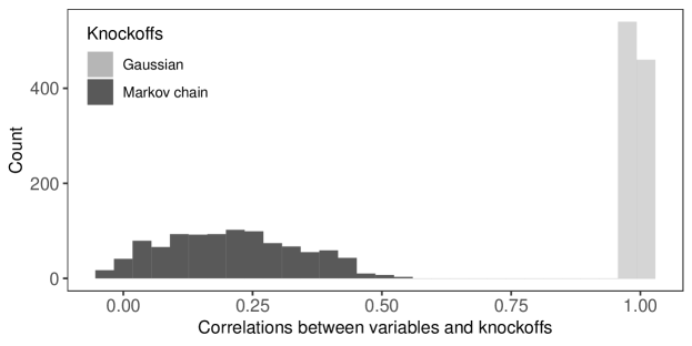
Figure 3: Histogram of the pairwise correlations between variables and knockoffs, $\text{Cor}(X_{j},\tilde{X}_{j})$, for $j\in\{1,\ldots,p\}$, for the same experiment as in Figure 2. The approximate Gaussian knockoffs are almost identical to the original variables and will thus have very little power in practice.

8 Sampling knockoffs

The conditional distribution of knockoffs $\tilde{X}$ given the observed $X$ is not uniquely defined for any fixed data distribution $F_{X}$ (Rosenblatt et al., 2019). For example, $\tilde{X}=X$ satisfies the required exchangeability properties, despite having no practical use. A continuous family of conditional knockoff distributions is known for Gaussian variables, in which case one is typically chosen by solving a semi-definite program to minimize the pairwise correlations between $X_{j}$ and $\tilde{X}_{j}$, in order to maximize power (Candès et al., 2018). Even though a similar optimization problem does not arise as naturally in the context of hidden Markov models, different constructions are available. For instance, the suggestion of Rosenblatt et al. (2019) to set $\tilde{Z}=Z$ in Algorithm 2 of Sesia et al. (2018) would also generate exact knockoffs, albeit more correlated with $X$.

The recent work of Romano et al. (2018) proposes an alternative machine that can produce approximate knockoffs in great generality, without making modeling assumptions on $F_{X}$ (Bottolo & Richardson, 2019; Rosenblatt et al., 2019). The approach of Romano et al. (2018) is based on deep generative models and it can be powerful because it is driven by the effort to make $\tilde{X}$ as uncorrelated with $X$ as possible in the spirit of Barber & Candès (2015). However, deep knockoffs are more computationally expensive and are not exactly exchangeable when applied to hidden Markov models. Whether ideas from our paper can be combined with those in Romano et al. (2018) to obtain an improved knockoff sampler is an open question. In any event, deep knockoffs may offer a practical solution for the analysis of other types of data for which a reliable model of $F_{X}$ is either unavailable or intractable.

9 Computational efficiency

We believe that a multivariate analysis with knockoffs is in principle feasible even for very large datasets (Rosenblatt et al., 2019), although some computational aspects of our pipeline can be improved. The computational cost of the algorithms for sampling knockoff copies of hidden Markov models described in this paper is $\mathcal{O}(npK^{2})$, where $K$ is the number of latent states. Even though this is not exorbitant compared to that of estimating $F_{X}$ and evaluating multivariate measures of feature importance, it can become important when $K$ is large (Marchini, 2019; Bottolo & Richardson, 2019; Rosenblatt et al., 2019). Moreover, all three of the major aforementioned steps in our variable selection procedure can be expensive when many samples must be considered. A solution mitigating this limitation will be presented soon, as we have developed a significantly faster implementation of our methods and we are applying it to the genetic analysis of the UK Biobank data (Bycroft et al., 2018). We will be excited to share the genotype knockoffs for this resource, as soon as we have been able to generate them with all the properties we have discussed here (Marchini, 2019). In any case, knockoffs are already more computationally efficient in this paper than the existing alternatives for high-dimensional conditional testing, such as the randomization test (Rosenblatt et al., 2019), discussed in Candès et al. (2018).

10 Aggregating dependent discoveries

We have observed in several numerical experiments that the results obtained from different realizations of the knockoffs can often be combined while empirically controlling the false discovery rate; e.g., keeping only those variables that are selected at least 50% of the times (Bogdan, 2017). Whether more stable procedures and rigorous results can be derived is still under investigation, since it is plausible that such simple heuristics may fail in certain cases. We are optimistic that future work will bring further improvements in this direction, even though aggregating the results of different dependent tests is a problem that goes well beyond the scope of knockoffs (Jewell & Witten, 2019). Most statistical findings are more or less randomized, as they involve some form of data splitting, resampling, cross-validation or simply the discretion of the practitioner to choose a model, use prior knowledge, or tune hyperparameters.

11 The statistical power of knockoffs

Methods based on knockoffs may enjoy substantial power as a result of the flexibility offered in the choice of the importance statistics. In fact, a variety of sparse estimators, cross-validation techniques, Bayesian models and very complex machine learning tools can be summoned at will to evaluate importance measures for the augmented set of original predictors and knockoffs. Of course, the choice of the most appropriate importance statistics for the problem is left to the user, who has to balance power and computational costs, and not dictated by the knockoff procedure. With this regard, we find the suggestion of Marchini (2019) particularly useful: it certainly seems promising to leverage the advantages of linear mixed model methodologies for the analysis of genome-wide association studies. For example, one can imagine using a screening procedure that is based on the results of linear mixed models on original and knockoff genotypes to obtain a smaller set of variables to pass on to a lasso estimation. We will certainly invest some effort in identifying which importance statistics are most effective and we would be thrilled to see other scientists contribute to this effort.

The argument made by Rosenblatt et al. (2019) in their hypothetical example to illustrate the potential lack of power of knockoffs rests on the assumption that knockoffs must rely on linear regression. Although this assumption is unjustified, knockoffs prove to be very successful even in this adversarial setting that they describe. In order to test this claim, we have implemented the experiment outlined in Rosenblatt et al. (2019), using $p=500$ variables divided in blocks of size 2 with internal correlations equal to $\rho=0.9$. The number of non-null variables is $|\mathcal{S}|=20$ and their signal amplitude is equal to $\beta_{j}=0.25$. The performance of knockoffs with Lasso statistics is compared to that of the linear regression method suggested by Rosenblatt et al. (2019), combined with the Benjamini-Hochberg procedure (Benjamini & Hochberg, 1995) at the nominal level $q=0.1$. This choice is intended to make the comparison with knockoffs as fair as possible, although the Benjamini-Hochberg procedure is not theoretically guaranteed to control the false discovery rate in this multivariate regression problem. The results reported in Figure 4 show that knockoffs are much more powerful than the proposed alternative, even though the experiment was designed to be “clearly unfavorable”, quoting from Rosenblatt et al. (2019).

The presence of strong correlations among the covariates always makes the variable selection problem harder, but it has no more effect on knockoffs than it would have on any other procedure, as shown in the experiment above. In general, knockoffs methods perform well for essentially two reasons: they can exploit powerful measures of variable importance and they can leverage prior information on the structure of the predictors. We leveraged predictor information in the experiment as $\tilde{X}$ was generated using knowledge of the covariance of $X$. As long as this information is available, at least approximately, knockoffs methods can prove powerful while controlling the false discovery rate. This justifies deployment in genome-wide association studies since a great deal of prior information is available about the structure of the explanatory variables.

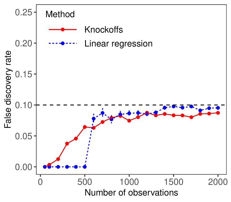
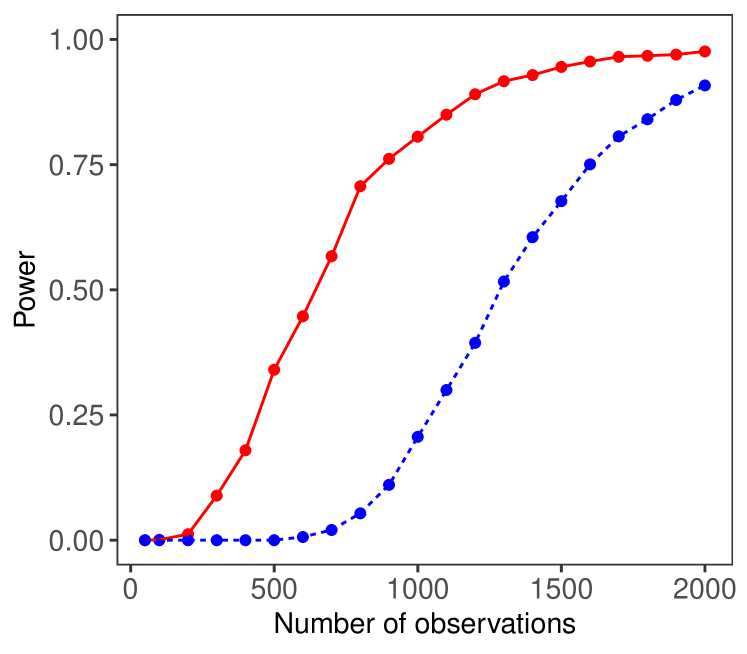
Figure 4: Numerical experiment comparing the performance of knockoffs and linear regression for variable selection with $p=500$ variables, in the adversarial setting designed by Rosenblatt et al. (2019) to be unfavorable to knockoffs. The false discovery rate (left) and power (right) are averaged over 1000 independent experiments. Both methods are applied at the nominal false discovery rate level $q=0.1$, although only knockoffs are rigorously guaranteed to control it.

12 Supplementary material

The code to reproduce the numerical simulations described in this discussion is available online at https://bitbucket.org/msesia/gene_hunting_discussion/.

References

- Barber & Candès (2015) Barber, R. F. & Candès, E. J. (2015). Controlling the false discovery rate via knockoffs. Ann. Statist. 43, 2055–2085.
- Barber et al. (2018) Barber, R. F., Candès, E. J. & Samworth, R. J. (2018). Robust inference with knockoffs. arXiv:1801.03896 .
- Battle et al. (2017) Battle, A., Brown, C. D., Engelhardt, B. E., Montgomery, S. B. et al. (2017). Genetic effects on gene expression across human tissues. Nature 550, 204–213.
- Benjamini & Hochberg (1995) Benjamini, Y. & Hochberg, Y. (1995). Controlling the false discovery rate: a practical and powerful approach to multiple testing. J. R. Statist. Soc. B 57, 289–300.
- Bogdan (2017) Bogdan, M. (2017). personal communication.
- Bottolo & Richardson (2019) Bottolo, L. & Richardson, S. (2019). Discussion of “Gene hunting with hidden Markov model knockoffs”. Biometrika 106, 19–22.
- Boyle et al. (2017) Boyle, E. A., Li, Y. I. & Pritchard, J. K. (2017). An expanded view of complex traits: from polygenic to omnigenic. Cell 169, 1177–1186.
- Buzdugan et al. (2016) Buzdugan, L., Kalisch, M., Navarro, A., Schunk, D., Fehr, E. & Buhlmann, P. (2016). Assessing statistical significance in multivariable genome wide association analysis. Bioinformatics 32, 1990–2000.
- Bycroft et al. (2018) Bycroft, C., Freeman, C., Petkova, D., Band, G., Elliott, L. T., Sharp, K., Motyer, A., Vukcevic, D., Delaneau, O., O’Connell, J., Cortes, A., Welsh, S., Young, A., Effingham, M., McVean, G., Leslie, S., Allen, N., Donnelly, P. & Marchini, J. (2018). The UK Biobank resource with deep phenotyping and genomic data. Nature 562, 203–209.
- Candès et al. (2018) Candès, E. J., Fan, Y., Janson, L. & Lv, J. (2018). Panning for gold: “model-X” knockoffs for high dimensional controlled variable selection. J. R. Statistic. Soc. B 80, 551–577.
- Dai & Barber (2016) Dai, R. & Barber, R. (2016). The knockoff filter for FDR control in group-sparse and multitask regression. In Proceedings of The 33rd International Conference on Machine Learning, M. F. Balcan & K. Q. Weinberger, eds., vol. 48 of Proceedings of Machine Learning Research. New York, New York, USA.
- Delaneau et al. (2012) Delaneau, O., Marchini, J. & Zagury, J.-F. (2012). A linear complexity phasing method for thousands of genomes. Nature Meth. 9, 179.
- Edwards et al. (2013) Edwards, S. L., Beesley, J., French, J. D. & Dunning, A. M. (2013). Beyond GWASs: illuminating the dark road from association to function. Am. J. Hum. Genet. 93, 779–797.
- Falush et al. (2003) Falush, D., Stephens, M. & Pritchard, J. K. (2003). Inference of population structure using multilocus genotype data: linked loci and correlated allele frequencies. Genetics 164, 1567–1587.
- Hoggart et al. (2008) Hoggart, C. J., Whittaker, J. C., De Iorio, M. & Balding, D. J. (2008). Simultaneous analysis of all SNPs in genome-wide and re-sequencing association studies. PLOS Genet. 4, 1–8.
- Hormozdiari et al. (2014) Hormozdiari, F., Kostem, E., Kang, E. Y., Pasaniuc, B. & Eskin, E. (2014). Identifying causal variants at loci with multiple signals of association. Genetics , genetics–114.
- J. DiCiccio & Romano (2016) J. DiCiccio, C. & Romano, J. (2016). Robust permutation tests for correlation and regression coefficients. J. Am. Statist. Assoc. 112.
- Jewell & Witten (2019) Jewell, S. W. & Witten, D. M. (2019). Discussion of “Gene hunting with hidden Markov model knockoffs”. Biometrika 106, 23–26.
- Kang et al. (2010) Kang, H. M., Sul, J. H., Service, S. K., Zaitlen, N. A., Kong, S., Freimer, N. B., Sabatti, C. & Eskin, E. (2010). Variance component model to account for sample structure in genome-wide association studies. Nature Genet. 42, 348–354.
- Katsevich & Sabatti (2017) Katsevich, E. & Sabatti, C. (2017). Multilayer Knockoff Filter: Controlled variable selection at multiple resolutions. ArXiv:1706.09375, forthcoming in Ann. Appl. Stat. .
- Klasen et al. (2016) Klasen, J. R., Barbez, E., Meier, L., Meinshausen, N., Buhlmann, P., Koornneef, M., Busch, W. & Schneeberger, K. (2016). A multi-marker association method for genome-wide association studies without the need for population structure correction. Nat. Commun. 7, 13299.
- Li & Stephens (2003) Li, N. & Stephens, M. (2003). Modeling linkage disequilibrium and identifying recombination hotspots using single-nucleotide polymorphism data. Genetics 165, 2213–2233.
- Marchini (2019) Marchini, J. L. (2019). Discussion of “Gene hunting with hidden Markov model knockoffs”. Biometrika 106, 27–28.
- Miller (1984) Miller, A. J. (1984). Selection of subsets of regression variables. J. R. Statistic. Soc. A , 389–425.
- O’Connell et al. (2014) O’Connell, J., Gurdasani, D., Delaneau, O., Pirastu, N., Ulivi, S., Cocca, M., Traglia, M., Huang, J., Huffman, J. E., Rudan, I. et al. (2014). A general approach for haplotype phasing across the full spectrum of relatedness. PLOS Genet. 10, e1004234.
- O’Connell et al. (2016) O’Connell, J., Sharp, K., Shrine, N., Wain, L., Hall, I., Tobin, M., Zagury, J.-F., Delaneau, O. & Marchini, J. (2016). Haplotype estimation for biobank-scale data sets. Nature Genet. 48, 817.
- Pritchard et al. (2000) Pritchard, J. K., Stephens, M. & Donnelly, P. (2000). Inference of population structure using multilocus genotype data. Genetics 155, 945–959.
- Romano et al. (2018) Romano, Y., Sesia, M. & Candès, E. J. (2018). Deep Knockoffs. ArXiv:1811.06687 .
- Rosenblatt et al. (2019) Rosenblatt, J. D., Ritov, Y. & Goeman, J. J. (2019). Discussion of “Gene hunting with hidden Markov model knockoffs”. Biometrika 106, 29–33.
- Scheet & Stephens (2006) Scheet, P. & Stephens, M. (2006). A fast and flexible statistical model for large-scale population genotype data: applications to inferring missing genotypes and haplotypic phase. Am. J. Hum. Genet. 78, 629–644.
- Sesia et al. (2018) Sesia, M., Sabatti, C. & Candès, E. J. (2018). Gene hunting with hidden Markov model knockoffs. Biometrika 106, 1–18.
- Spain & Barrett (2015) Spain, S. L. & Barrett, J. C. (2015). Strategies for fine-mapping complex traits. Human molecular genetics 24, R111–R119.
- Visscher et al. (2017) Visscher, P. M., Wray, N. R., Zhang, Q., Sklar, P., McCarthy, M. I., Brown, M. A. & Yang, J. (2017). 10 years of gwas discovery: biology, function, and translation. Am. J. Hum. Genet. 101, 5–22.
- Wu et al. (2007) Wu, Y., Boos, D. D. & Stefanski, L. A. (2007). Controlling variable selection by the addition of pseudovariables. J. Am. Statist. Assoc. 102, 235–243.
- Zhang et al. (2010) Zhang, Z., Ersoz, E., Lai, C.-Q., Todhunter, R. J., Tiwari, H. K., Gore, M. A., Bradbury, P. J., Yu, J., Arnett, D. K., Ordovas, J. M. et al. (2010). Mixed linear model approach adapted for genome-wide association studies. Nature Genet. 42, 355.