Reactive sensing and multiplicative frame super-resolution

Abstract.

The problem is to evaluate the behavior of an object when primary sources of information about the object become unavailable, so that any information must be obtained from the intelligent use of available secondary sources. This evaluative process is reactive sensing. Reactive sensing is initially viewed in terms of spatial super-resolution. The theory of reactive sensing is based on two equivalent ideas, one physical and one mathematical. The physical idea models volume, e.g., engine volume in the case of analyzing engine health, and the sensitivity of sensors to such volume. The mathematical idea of multiplicative frames provides the factorization theory to compare quantitatively such volume and sensitivity. This equivalence is the foundation for reactive sensing theory and its implementation.

1. Introduction

1.1. Background and modeling

Sensing problems such as those dealing with RADAR, SONAR, and general engine health, in the context of disabled primary sensors and in noisy environments, led us to the theory of reactive sensing. Our formulation of this theory necessitates the understanding of secondary sensors in evaluating primary objects. With this point of view, we see that reactive sensing can be thought of in terms of spatial super-resolution, e.g., [21], [13], [31], [32], [23], [30]. (This is in contrast to recent advances in spectral super-resolution, e.g., [10], [11].[7].) In fact, the secondary sensors can be considered analogous to the role of obtaining a high resolution (HR) image from observed multiple low-resolution (LR) images. In this case, the multiple LR images represent different “snapshots” of the same scene, and can be combined to give the desired HR image, see [13], Chapter 4. In our case, the LR images correspond to secondary sensors and the HR image corresponds to the primary object, that could be disabled or whose primary sensor is not functioning.

Notwithstanding this significant connection between our formulation of reactive sensing and spatial super-resolution, we do not use any of the usual super-resolution methodology in developing our theory. For example, in the case of engine health, the understanding of secondary sensors is based on a physical modeling of inherent engine volume or vibration and the sensitivity of sensors to such volume, We show that this physical modeling is equivalent to a mathematical modeling formulated in terms of what we call multiplicative frames. This also leads us to the concept of sensing scenario health space determined by data dependent dimension reduction.

1.2. Idea and techniques

Our main objective in reactive sensing is to evaluate the behavior of an object when primary sources of information about the object become unavailable so that any information must be obtained from the intelligent use of available secondary sources. For example, if our object is an engine evaluated by a sensor and the sensor is disabled, we wish to quantify to what extent neighboring sensors, that have primary tasks of their own, can evaluate the behavior of the engine.

The idea and techniques we shall introduce to understand reactive sensing, at the level of obtaining quantifiable and computationally useful results, involve an interleaving of the following:

• The theory of frames, see Section 4 and Subsection 5.1; and

• Sensing scenario health space, see Section 3.

The theory of frames has a long history, based on the work of Paley-Wiener, Beurling, and Henry Landau, and was explicitly developed by Duffin and Schaeffer (1952). In recent decades there has been an explosion of activity related to the emergence of Gabor (time-frequency) and wavelet theories, as well as to applicability in the context of noise reduction, robust signal decomposition, and numerical stability. See [18], [6], Chapters 3 and 7, [14], and [25], [26]. The interaction of frame theory with the data sets we analyze has led us to develop a theory of multiplicative frames.

Health space can be described functionally as a space where decision making algorithms operate to provide required data analysis. Its dimension will be given by the number of parameters required to perform the analysis. The name health space is used because of questions about machine health, but the same notion can be applied in other detection and classification contexts, see Definition 3.1 and Remark 3.2 for specifics on our point of view.

1.3. Theme and implementation

A natural strategy inherent in implementing the idea and technique of Subsection 1.2 is to choose an efficient method of finding relevant data and discarding redundant information and noise. While this paradigm may work well when all of the data streams are available and all of the sensors are operating, problems can arise when some of the data streams are unavailable because of various possible failures. The theme of reactive sensing is to construct mappings of the data streams that are robust under sensor failure. A critical aspect of our mathematical approach for this construction, necessitating the use of multiplicative frames, is that an individual sensor may be capable of reporting on parameters which are not its primary responsibility.

Our theme leads to a genuine implementation in Section 6 by the following process. Once we have shown the equivalence of our physical modeling with multiplicative frames (Sections 3 and 4.2), we define frame mappings (Definition 5.2 b) which allow us to prove fundamental theorems on the existence of multiplicative frames in Section 5. The definition is technical but motivated by the inherent over-completeness of frames. The definition itself and these theorems are essential for the quantitative results in Section 6, as well as in a host of other applications.

1.4. Outline

We begin in Section 2 with some relevant examples. These examples provide the backdrop for the mathematical model we formulate in Section 3 for the physical setting of a reactive sensing scenario.

It is in Section 3 that we introduce the notions of a separable sensing scenario and health space, that are essential for a useful theory of reactive sensing. Further, the physical notions of radiativity and dominance are quantified in terms of the notions of volume and sensitivity used in the definition of the model. The examples in Section 2 and the consequent model of Section 3 lead to the theory of frames as a natural tool for effective reactive sensing.

Subsection 4.1 gives a background on frames, with a comparison to bases, in the context of our setting. It is in Subsection 4.2 that we introduce multiplicative frames. This is a mathematical concept directly formulated because of the physical implications of the model of Section 3, see especially the paragraph before Definition 3.1, Definition 3.1 itself, Example 3.3, Remark 3.5, Remark 3.9, and Remark 3.15. In fact, our mathematical constructions of multiplicative frames in Theorem 4.5, Corollary 4.6, and Theorem 5.12, that of themselves are independent of reactive sensing, depend essentially on the reactive sensing ideas of radiativity and dominance defined in Definition 3.8.

Section 5 presents the theory of reactive sensing in which multiplicative frames play an essential role. It is here that we define and analyze basis and frame mappings. In the context of super-resolution, individual LR sensor outputs that are combined by means of basis mappings do not improve resolution, i.e., do not lead to reconstructing the primary HR object, described in Subsection 1.1. On the other hand, frame mappings, by their over-complete nature, piece together LR sensor outputs to optimize the chances of such HR reconstruction.

The DFT plays a fundamental role in our exposition and for our explanations. As such, we give DFT examples throughout as various notions are introduced. In particular, we give a simplified version of the turbine assembly example, Example 2.3, in terms of the DFT.

In Subsection 6.2 we construct a data base, and in Subsection 6.4, we give DFT turbine simulations that give proof of concept of our reactive sensing theory using this data base. Using the signal-to-noise (SNR) as a metric, we verify improvement in fault detection in the case of sensor failure. We also note that this improvement comes at the expense of lowering SNR in a controlled fashion when all sensors are working. This is the content of Subsection 6.6.

The epilogue, Section 7, gives a summary of the salient features of reactive sensing with remarks on future tasks.

2. Examples

Example 2.1 (RADAR).

Consider a collection of RADAR sites which is responsible for detecting incoming targets in a given sensing scenario, see Figure 1. Doppler and range returns for a target might be at the limit of detectability for RADARs $A$ and $C$ but be within the main analysis area for RADAR $B.$ However, if RADAR $B$ is disabled, the data from RADARs $A$ and $C$ might be combined to give a noisier but adequate return from the target. Indeed, for the situation described in Figure 1, a target at $X$ can be detected by both RADARs $A$ and $B.$ While the return from RADAR $A$ is noisier than that from $B,$ it may still be sufficient to provide adequate detectability, see Example 3.19 dealing with non-harmonious scenarios. In fact, this may allow RADAR $B$ to be temporarily repurposed, repaired, or relocated as required, while still maintaining an acceptable level of coverage, see [36], [28], [16], [37], [29], [34].

Figure 1. RADAR scenario

Example 2.2 (SONAR).

Similarly, consider a SONAR sensing scenario, where a section of coastal waters is observed by two SONAR arrays, $A$ and $B,$ see Figure 2. Each array has main beams, where the signal strength is high compared to the noise, as well as beams near endfire, where there is significantly more noise, see, e.g., [38]. These beams close to endfire are illustrated in Figure 2 by the boundary ”petals” in each collection of beams. If we consider both of these arrays as sensors, then array $A$ would be primarily responsible for reporting a threat in its main beams that might be near the endfire beams of array $B$. However, in the event of a failure in array $A,$ array $B$ could also sense the target, although with some degradation due to the additional noise, see Example 3.19 dealing with harmonious scenarios.

Figure 2. Target $X$ as sensed by SONAR arrays $A$ and $B$

Example 2.3 (The DFT and a multi-sensor scenario).

A third example concerns the mechanical health of a complex machine. Consider a machine with several rotating turbines, each attached to several gears and additional rotating shafts to form a collection of turbine assemblies, e.g., [19], [20]. Assume there are vibration sensors attached to each turbine assembly and that each assembly has unique spectral characteristics. A concrete example might be a multi-engine airplane where each of the engine’s turbines is associated with a given sensor, see Section 6.

The sensor attached to a given turbine assembly will have primary responsibility for the frequencies associated with that assembly. This notion of primary responsibility will be quantified more precisely in Subsection 3.1, and takes into account that each sensor will also pick up vibrations from other nearby assemblies at a substantially lower volume. If a sensor fails, it may be possible to use data from the remaining sensors to report characteristics of the failed sensor’s turbine assembly.

It is this point of view that led us to introduce the theory of frames. In fact, this type of data reconstruction is only possible if the fault detection scheme operates with a frame theoretic representation of the vibration parameters. With a basis representation, the loss of a sensor causes a loss of all data associated with that turbine assembly. Indeed, for an airplane, it is important to distinguish between an impact which causes the loss of a sensor and an impact which causes the loss of an engine.

The DFT provides a natural technical tool with which to analyze this particular multi-sensor scenario, see the DFT Example 3.3 and Section 6.

3. A mathematical model for reactive sensing

3.1. Separable sensing scenario

We wish to analyze the sensing problems described in Subsection 1.3 and Section 2 with a mathematical model. To this end, we let $S$ be a set, that we call a set of parameters. To $S$ we associate $N$ sensors, $s_{j},\ j=1,...,N,$ that map subsets of $S$ to their values at a fixed time $k=1,...,K$. Each sensor $s_{j}$ is defined on some subset $T_{j}$ of $S$. To evaluate completely the impact of the parameters in $S$, we require that $\bigcup_{j=1}^{N}T_{j}=S$, i.e., the $T_{j},\,j=1,\ldots,N$, form a covering of $S$.

Each sensor $s_{j}$ will bear primary responsibility for reporting values on some subset $S_{j}\subseteq T_{j}$ in the sense that $S_{j}\bigcap S_{\ell}=\emptyset,$ where $1\leq j,\ell\leq N$ and $j\neq\ell,$ and the values of $s_{j}$ on $T_{j}\setminus S_{j}$ reflect information gathered by $s_{j}$ for parameters disjoint from $S_{j}.$ We assume that the primary responsibility for each parameter is given to one sensor, and that the $S_{j},j=1,\ldots N,$ form a partition of $S$, i.e., $\bigcup_{j=1}^{N}S_{j}=S$ and $S_{j}\bigcap S_{\ell}=\emptyset,$ where $0\leq j,\ell\leq N$ and $j\neq\ell.$

The cardinality of any set $X$ is denoted by ${\rm card}\,(X),$ and $M$ will denote ${\rm card}\,(S).$

In this formulation of a sensor $s_{j}$ as a mapping, we have to be precise about the role of time $k.$ As such, each $s_{j}$ assigns values to the elements of $T_{j}$ at a given time index $k$, i.e., $s_{j}:T_{j}\times\{1,...,K\}\rightarrow{\mathbb{C}}^{M}$, where we write $s_{j}(f,k)=v_{j,k}(f).$ Further, if $f\notin T_{j},$ then we define $s_{j}(f,k)=0.$ Thus, $v_{j,k}\in{\mathbb{C}}^{M}.$ We use the notation, $f\in\{1,\ldots M\},$ to think of the frequency domain of the DFT, even though our theory is far more general.

Given a set $S$ with partition $\{S_{j}\}$, covering $\{T_{j}\}$, and mappings $s_{j}.$ We refer to $S$ as a sensing scenario, see Figure 3.

Figure 3. Sensing scenario $S:$ In (a), $S$ is the rectangle with two disjoint subsets, $S_{1}$ and $S_{2};$ in (b), $T_{1}$ is the hashed area; and in (c), $T_{2}$ is the hashed area.

If a parameter $f$ is in $T_{j}$ then, at each time $k,$ sensor $s_{j}$ assigns a value to it. We can think of this value as the response that sensor is reporting for the parameter, $f,$ at time, $k.$ This process is usually the natural result of two effects: the inherent intensity (or volume or loudness) of the scenario at which the parameter is being generated, and the sensitivity of the sensor to that parameter. In this regard see Example 3.3 and Remark 3.9. As such, we make the following definition (Definition 3.1). The factorization in this definition and its physical motivation with regard to volume and sensitivity are the rationale for our notion of multiplicative frames, defined in Section 4.2. The factorization in Definition 3.1, part b, “without the hats” is what occurs in a health space, ${\mathbb{C}}^{n}.$

Definition 3.1 (Separable sensing scenario and health space).

Let $S$ be a sensing scenario.

a. $S$ is pre-separable if for each $1\leq f\leq M$, $1\leq j\leq N$, and $1\leq k\leq K$, we have the factorization,

$$v_{j,k}(f)={\widehat{\gamma}}_{j}(f)\,{\widehat{\alpha}}_{k}(f).$$

b. A pre-separable sensing scenario $S$ is separable if there are a positive integer $n$ and a mapping,

$$H:{\mathbb{C}}^{M}\longrightarrow{\mathbb{C}}^{n},$$

such that, for each $i=1,\ldots,n$, $j=1,\ldots,N$, and $k=1,\ldots,K$, the image, $H(v_{j,k})\in{\mathbb{C}}^{n}$, factors as

$$H(v_{j,k})(i)={\gamma}_{j}(i)\,{\alpha}_{k}(i),$$

where ${\alpha}_{k},{\gamma}_{j}\in{\mathbb{C}}^{n}$, and such that $H(0)=0\in{\mathbb{C}}^{n}$, see Definition 5.2.

$H$ is a health space mapping, and ${\mathbb{C}}^{n}$ is a health space.

Remark 3.2 (Rationale for health space).

a. Motivation. The motivation behind formulating the notion of health space is to construct a lower dimensional, space, ${\mathbb{C}}^{n}$, in which we can effectively analyze a separable sensing scenario $S$. The dimension $n$ is related to the general theory of dimension reduction, although our implementation in Section 6 only uses a type of PCA. The health space ${\mathbb{C}}^{n}$ and health space mapping $H$ are part and parcel of the concept of a sensing scenario. Indeed, if the number of sensors and parameters is small enough to be analyzed without dimension reduction, there would be no need to develop the theory further. Hence, we shall always consider a sensing scenario with health space ${\mathbb{C}}^{n}$ and health space mapping $H:{\mathbb{C}}^{M}\longrightarrow{\mathbb{C}}^{n}$.

b. The size of $n$. The dimension $n$ should be taken as small as possible, and we must have $n<NM$ or there would be no point in applying reactive sensing theory. Usually, the size of $n$ is determined by the analysis algorithms that will be applied.

For example, suppose we have a scenario where the frequency domain output from a group of vibration sensors is used to diagnose the mechanical health of a device. There may be many components with complex spectral characteristics that need to be evaluated to detect or classify a fault. In this case $n$ may be comparatively large while the number of sensors, $N$, might not be. This is precisely the scenario in Section 6 where $n=28$ and $N=4$.

On the other hand, consider a collection of inexpensive sensors each of which is detecting an energy spike. This might be the case if the sensors were sprinkled across a roadway with the intent of monitoring the amount of traffic. Here $n$ could be small (maybe even 1), while $N$ could be large.

3.2. Examples of separable sensing scenaios

Example 3.3 (A DFT separable sensing scenario).

a. A useful example, of which Example 2.3 is a prototype, results from considering sensors $s_{j}$ that perform a DFT on blocks of $2^{r}$ points. At a time, $k,$ for $k=1,\ldots,K,$ each sensor, $s_{j}$ , will report $2^{r}$ values for the DFT frequency bins. Thus, we can define $S$ to be the set of $2^{r}$ parameters, $f,$ and so $M={\rm card}(S)=2^{r}.$ The sets, $T_{j}$ and $S_{j},$ will be a covering and partition of $S,$ respectively. For example, if we have acoustic or vibration sensors, it may be that $T_{j}=S$ since all sensors hear every frequency, but the sets $S_{j}$ consist of only those frequencies for which sensor $s_{j}$ is the best value, e.g., the loudest or highest SNR value. It is for this reason that we introduced the notion of primary responsibility.

b. In the case of sensors attached to the turbine assemblies of Example 2.3, we shall provide numerical simulations in Section 6 quantifying our formulation of reactive sensing. In fact, we consider each $S_{j}$ in the sensing scenario $S$ as the set of frequencies generated by the $j$-th engine. Thus, each $s_{j}$ is associated with the same engine and maps the frequencies to their values recorded by the sensor. The factor ${\widehat{\gamma}}_{j}(f)\in{\mathbb{C}}$ represents the ability of $s_{j}$ to ”hear” the frequency $f$ of $S_{j};$ and the factor ${\widehat{\alpha}}_{k}(f)\in{\mathbb{C}}$ represents the ”loudness” of the scenario $S$ at frequency $f$ and time $k,$ see Remark 3.9 for a fuller treatment of this mathematical and physical modeling.

Proposition 3.4 (Linear separable sensing scenario – constant ${\widehat{\alpha}}_{k}(f)$).

Let $S$ be a pre-separable sensing scenario with the property that, for each $1\leq k\leq K$,

(1) $$\exists\,{\widehat{\alpha}}_{k}\in{\mathbb{C}}\;{\rm such\,that}\;\forall f,f^{\prime}\in\{1,...,M\},\quad{\widehat{\alpha}}_{k}(f)={\widehat{\alpha}}_{k}(f^{\prime})={\widehat{\alpha}}_{k}.$$

Let $H$ be a linear mapping defined by

$$H:{\mathbb{C}}^{M}\rightarrow{\mathbb{C}}^{n},$$

$$H(x)=Ax,$$

where A is an $n\times M$ matrix of complex numbers. Then, $S$ is a separable sensing scenario and $H$ is a health space mapping in the sense of Definition 3.1.

Proof.

Let $A=[a_{i,f}]$ where $i\in\{1,...,n\}$ and $f\in\{1,...,M\}$. Since $S$ is pre-separable and by (1), we have $v_{j,k}(f)={\widehat{\gamma}}_{j}(f){\widehat{\alpha}}_{k}(f)={\widehat{\gamma}}_{j}(f){\widehat{\alpha}}_{k}.$ Therefore, for each $j=1,\ldots,N$ and $k=1,\ldots,K$, we can apply $H$ as follows:

$$H(v_{j,k})(i)=\sum_{f=1}^{M}a_{i,f}v_{j,k}(f)=\sum_{f=1}^{M}a_{i,f}{\widehat{\gamma}}_{j}(f){\widehat{\alpha}}_{k}=\big{(}\sum_{f=1}^{M}a_{i,f}{\widehat{\gamma}}_{j}(f)\big{)}{\widehat{\alpha}}_{k}=\gamma_{j}(i)\alpha_{k}(i),$$

where we set $\gamma_{j}=A{\widehat{\gamma}}_{j}\in{\mathbb{C}}^{n}$ and $\alpha_{k}(i)={\widehat{\alpha}}_{k}.$ This completes the proof. ∎

Remark 3.5 (Physical systems with and without constant ${\widehat{\alpha}}_{k}(f)$).

Condition (1) requiring ${\widehat{\alpha}}_{k}$ to be constant is reasonable in some physical systems. For example, linear amplifiers will have this property over their intended operational bandwidth, see [39]. However, some physical processes do not have this property. In particular, signal strength loss from free space propagation in both the radio frequency and acoustic regimes is highly dependent on frequency, e.g., [33]. High frequencies are more attenuated than low frequencies, and this means that the ${\widehat{\alpha}}_{k}(f),f\in\{1,\ldots,M\}$, values may vary. Hence, the DFT example in Section 6 will not satisfy condition (1). On the other hand, if the matrix $A$ of Proposition 3.4 is sufficiently simple, then condition (1) is not necessary to ensure that $S$ is separable, as the following result shows.

Proposition 3.6 (Linear separable sensing scenario – matrix constraint).

Let $S$ be a pre-separable sensing scenario. Let $H$ be a linear mapping defined by

$$H:{\mathbb{C}}^{M}\rightarrow{\mathbb{C}}^{n},$$

$$H(x)=Ax,$$

where A is an $n\times M$ matrix of complex numbers. Suppose the rows of $A$ are constant multiples of rows taken from the rows of the $M\times M$ identity matrix. Then, $S$ is a separable sensing scenario and $H$ is a health space mapping in the sense of Definition 3.1.

Proof.

The $i$-th row of $A$ consists of $M-1$ zeros and one non-zero entry at a position we shall call $f_{i}$, that is, $a_{i,f}=0$ for all $f\neq f_{i}$ and $a_{i,f_{i}}\neq 0$. Therefore, for each $j=1,\ldots,N$ and $k=1,\ldots,K$, we can apply $H$ as follows:

$$H(v_{j,k})(i)=\sum_{f=1}^{M}a_{i,f}v_{j,k}(f)=a_{i,f_{i}}v_{j,k}(f_{i})=a_{i,f_{i}}{\widehat{\gamma}}_{j}(f_{i}){\widehat{\alpha}}_{k}(f_{i})=\gamma_{j}(i)\alpha_{k}(i),$$

where we set $\gamma_{j}(i)=a_{i,f_{i}}{\widehat{\gamma}}_{j}(f_{i})$ and $\alpha_{k}(i)={\widehat{\alpha}}_{k}(f_{i})$. This completes the proof. ∎

Remark 3.7 (Connection with DFT example).

Propositions 3.4 and 3.6 are relevant for showing that the mathematical techniques developed here will be applicable to the DFT scenario of Example 3.3 and Section 6. In particular, Proposition 3.6 shows that the projection mapping described in Section 6 is a health space mapping for a separable sensing scenario. Further, the proof of Proposition 3.4 shows that certain practicalities for dealing with real systems will not cause problems. For example, spectral lines that fall between DFT bins might require weighted averaging of adjacent values of the DFT output. Since these values correspond to adjacent frequencies, we can assume ${\widehat{\alpha}}_{k}(f)\approx{\widehat{\alpha}}_{k}(f+1),$ and the proof of Proposition 3.4 assures separability.

3.3. Radiative, dominant, and harmonious separable sensing scenario

Definition 3.1 allows us to quantify certain natural properties of the sensing scenario. In particular, it allows us to distinguish between a failed sensor and a failed component. It also allows us to quantify the notion of a sensor bearing primary responsibility for a particular parameter and for a parameter to be heard by more than one sensor. In order to justify these claims, we make the following definitions.

Definition 3.8 (Radiative and dominant separable sensing scenario).

Let $S$ be a separable sensing scenario, and let $i\in\{1,\ldots,n\}.$

a. $S$ is i-radiative if

$$\exists\,k_{i}\in\{1,\ldots,K\}\;\text{ such that }\;{\alpha}_{k_{i}}(i)\neq 0.$$

b. $S$ is i-dominant if

$$\exists\,j_{i}\in\{1,\ldots,N\}\;\text{ such that }\;{\gamma}_{j_{i}}(i)\neq 0;$$

and it is strongly i-dominant if

$$\exists\,j_{i}\in\{1,\ldots,N\}\text{ such that }\forall\ell\neq j_{i},\hskip 14.45377pt|{\gamma}_{j_{i}}(i)|>(N-1)|{\gamma}_{\ell}(i)|,$$

where $N$ is the number of sensors.

Remark 3.9 (Rationale for radiativity and dominance).

a. We have chosen the word, radiative, from the notion that in order for a parameter to be sensed, e.g., for a spectral line of a DFT to register at a given sensor, the object must radiate some sort of energy, viz., the $\widehat{{\alpha}}s$. Similarly, we have chosen the word, dominant, since the sensor which bears primary responsibility for reporting a parameter must be able to see/hear it loudly, viz., the $\widehat{{\gamma}}s.$ Naturally, if the object stops sending out energy, no sensor could detect it. Thus, in the case of engines (see Section 6), radiativity has to do with producing noise while dominance has to do with hearing the noise at the sensor.

b. Under a mild condition about the existence of non-zero elements, we have that if a sensor bears primary responsibility for a parameter, then the given separable sensing scenario $S$ is $i$-dominant for some $i$. To see this, suppose we are given a sensor, $s_{j}$, that bears primary responsibility for a parameter, $f\in\{1,\ldots,M\}$, i.e., $f\in S_{j}$. Then, consider the $1$-dimensional subspace ${\mathbb{C}}_{f}={\mathbb{C}}\subseteq{\mathbb{C}}^{M}$ generated by the canonical basis vector for ${\mathbb{C}}^{M}$ with a $1$ in the $f$ position. Since $H:{\mathbb{C}}^{M}\longrightarrow{\mathbb{C}}^{n}$ and ${\mathbb{C}}_{f}\subseteq{\mathbb{C}}^{M}$, we have that $H({\mathbb{C}}_{f})$ is a subset of ${\mathbb{C}}^{n}$. Therefore, if we assume further that $H({\mathbb{C}}_{f})$ has a non-zero element $H(v_{j,k})\in{\mathbb{C}}^{n},$ then

$$\exists i\in\{1,\ldots,n\}\;\text{such that}\;H(v_{j,k})(i)\neq 0;$$

and so

$$\gamma_{j}(i)\neq 0,$$

by the definition of the health space mapping $H$. Consequently, with $j=j_{i}$, we see from Definition 3.8 that $S$ is i-dominant for this $i$.

c. Of course, as the name implies, we would usually like to choose the $j_{i}$ in the definition of $i$-dominance so that $\gamma_{j_{i}}(i)$ is maximal in some sense. However, there are instances, particularly when there are noise considerations in the sensor output, when this may not be the case. For example, the largest $\gamma_{j_{i}}$ may also be significantly noisier, and possibly have a lower SNR, than another choice.

Figure 4. Dominance vs SNR

Example 3.10 (Dominance vs SNR).

Recall that SNR is defined as the ratio of the power of the desired signal to the background noise power, generally measured on a logarithmic scale in terms of decibels (dB), i.e.,

$${\rm SNR}={\rm P}_{{\rm signal}}/{\rm P}_{{\rm noise}}={\rm P}_{{\rm signal},{\rm dB}}-{\rm P}_{{\rm noise},{\rm dB}},$$

where ${\rm P}_{{\rm signal},{\rm dB}}=10\,{\rm log}_{10}({\rm P}_{{\rm signal}})$ and ${\rm P}_{{\rm noise},{\rm dB}}=10\,{\rm log}({\rm P}_{\rm noise})$ for signal and noise power, respectively.

As an example of the effect of SNR considerations on dominance, consider a situation, where there are 2 sensors, a signal source and a noise source, arranged in a line as in Figure 4. The first sensor, $s_{1},$ is located at a distance $d$ from the noise source and the signal source. The second sensor, $s_{2}$, is located at a distance $2d$ from the signal but $4d$ from the noise. This setup works equally well for both acoustic and RF sensing modeling, as long as we assume that the signal and noise propagate according to free space propagation, see [33]. According to such propagation, if the distance between the source and the sensor doubles, the received power level will decline by a factor of 4. Thus, if the signal strength at $s_{1}$ is ${\bf s}$, then the signal strength of $s_{2}$ will be ${\bf s}/4$. Hence, if signal strength were the only determining factor, then $\gamma_{1}$ would be maximal, and consequently it would be the obvious choice for a dominant value. However, if the signal strength of the noise at $s_{1}$ is ${\bf N}$, then, according to free space propagation, the noise power at $s_{2}$ will be ${\bf N}/16$. Therefore, if we compute SNR values, then the SNR at $s_{1}$ is ${\bf s}/{\bf N},$ while at $s_{2}$ it is $({\bf s}/4)/({\bf N}/16)=4{\bf s}/{\bf N}$. Thus, if SNR is a consideration, it is not unreasonable to choose $\gamma_{2}$ as the dominant value.

Example 3.11 (Primary responsibility).

The canonical example of primary responsibility is given by the DFT scenario described in Sections 6.2 and 6.4. There, the health space mapping, H, simply picks out the n significant frequencies from the M-point DFT. Thus, H is a projection mapping. In this case of the DFT, the parameters for which a sensor bears primary responsibility are the frequencies in $\{1,\ldots,M\}$ for which that sensor gives significant information. These frequencies will be mapped by the projection mapping onto the non-zero elements of ${\mathbb{C}}^{n}$. In fact, this defines an explicit mapping of only the significant frequencies, $f\in\{1,...,M\},$ mapping into ${\mathbb{C}}^{n}.$

We want to quantify the idea described in Example 3.11. In particular, given a separable sensing scenario with health space mapping H and health space ${\mathbb{C}}^{n}$, we wish to allow ${\mathbb{C}}^{n}$ to inherit the primary responsibility attributes available in ${\mathbb{C}}^{M}$. To this end, in Definition 3.12 we shall define notation for various parameters and sets of indices that are needed to quantify dominance, see Definition 3.14, and then to define harmonious scenarios, see Definition 3.16.

Definition 3.12 (Subsets of $\{1,\ldots,n\}$ for a separable sensing scenario).

Let $S$ be a separable sensing scenario.

a. Consider the vectors, $H(v_{j,k})\in{\mathbb{C}}^{n},$ where $1\leq j\leq N$ and $1\leq k\leq K$. For each $j=1,\ldots,N,$ construct the set

$$J_{j}=\{i\in\{1,\ldots,n\}:\exists k=k(i)\in\{1,\ldots,K\}\;\text{such that}\,H(v_{j,k})(i)\neq 0\},$$

see Figure 5.

A subset $J_{j}$ could be the empty set. Without loss of generality, we can assume that each $i\in\{1,\ldots,n\}$ can be found in at least one such set of indices. If not, then for that $i$,

$$\forall j,k,\quad H(v_{j,k})(i)=0,$$

in which case the health space mapping could be improved by projecting down to ${\mathbb{C}}^{n-1}$, eliminating the index $i$ altogether.

Further, we could have $J_{j}\cap J_{j^{\prime}}\neq\emptyset$ for some $j\neq j^{\prime}.$ We note here that the $J_{j}$ sets form a covering of the set $\{1,...,n\}$ in much the same way as the sets $T_{j}$ form a covering of $S$, see the beginning of Subsection 3.1.

b. We now wish to construct sets, $I_{j}$, of indices that correspond to the partition $\{S_{j}\}$. $I_{j}$ will have cardinality ${\rm card}\,(I_{j})=n_{j}$, and we would like $\sum_{j=1}^{N}n_{j}=n$. As such, for each $j=1,\ldots,N,$ we choose sets $I_{j}=\{i_{\ell,j}:\ell=1,...,n_{j}\}\subseteq J_{j},\,I_{j}\subseteq J_{j},$ with the properties that $\{I_{j}\}$ is a disjoint collection and $\bigcup_{j=1}^{N}\{I_{j}\}=\{1,...,n\},$ see Figure 6. We note that some of the $I_{j}$ can be the empty set even when $J_{j}\neq\emptyset$; in this case $n_{j}=0$.

Summarizing, we have that

(2) $$\forall i\in\{1,\ldots,n\},\;\exists j=j(i)\in\{1,\ldots,N\}\,\text{and}\,\ell\in\{1,\ldots,n_{j}\}\,\text{such that}\,i\in I_{j}\,{\rm and}\,i=i_{\ell,j},$$

and

(3) $$\forall i=i_{\ell,j}\in I_{j},\,\exists k=k(i)\in\{1,\ldots,K\}\,\text{such that}\,H(v_{j,k})(i_{\ell,j})\neq 0.$$

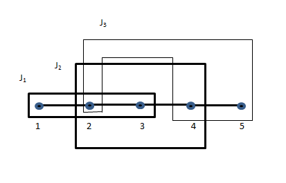
Figure 5. Sets $J_{1}$, $J_{2}$, $J_{3}$

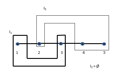
Figure 6. Sets $I_{1}$, $I_{2}$, $I_{3}$

Example 3.13 (Subsets of $\{1,\ldots,n\}$ for a separable sensing scenario).

We illustrate the relationship between the sets $I_{j}$ and $J_{j}$, see Figures 5 and 6. Consider a case where $n=5$ and $N=3$ We could have sets $J_{1}=\{1,2,3\}$, $J_{2}=\{2,3,4\}$, and $J_{3}=\{2,4,5\}$. We may then choose $I_{1}=\{1,3\}$, $I_{2}=\emptyset$, and $I_{3}=\{2,4,5\}$, in which case we have $n_{1}=2$, $n_{2}=0$, and $n_{3}=3$, so that $n_{1}+n_{2}+n_{3}=5=n$.

Definition 3.14 (Operational sensors).

Given the set-up of Definition 3.12, we have that $H(v_{j,k})(i)\neq 0$ for $i\in I_{j}$ and so $\gamma_{j}(i)\neq 0$ as well. In this case we shall say that the sensor $s_{j}$ is operational. If something goes wrong with the sensor, some or all of the $\gamma$s will be affected. We say that $s_{j}$ is non-operational if

$$\exists\ell\in\{1,\ldots,n_{j}\}\neq\emptyset\quad\text{such that}\quad\gamma_{j}(i_{\ell,j})=0.$$

Remark 3.15.

a. [$I_{j}$ and primary responsibility] There is a connection between the $I_{j}$ of Definition 3.12 and the notion of primary responsibility. We noted in Remark 3.9b that if a sensor $s_{j}$ bears primary responsibility for a parameter, $f$, then the scenario is $i$-dominant for some $i=i(j,f)$. In particular, we showed the existence of an $i$ for which $H(v_{j,k})(i)\neq 0$, where $k$ arises in Remark 3.9b. We would like this $i$ to be an element of $I_{j}$. However, this may not be possible since there may be another parameter, $f^{\prime}$, for which a sensor $s_{j^{\prime}}$ bears primary responsibility and for which $f^{\prime}$ gives rise to the same value of $i$.

b. [Non-operational sensors] Clearly, the failure of a sensor, i.e., a sensor becoming non-operational, could have a dramatic affect on the sensing scenario. In particular, if sensor $s_{j}$ becomes non-operational, then $\gamma_{j}(i_{\ell,j})=0$ implies that the scenario may no longer be $i$-dominant for $i=i_{\ell,j}$. Indeed, this will precisely be the case if there is no $j^{\prime}\neq j$ for which $i_{\ell,j}\in J_{j^{\prime}}$. Alternatively, however, it may be that there does exist such a $j^{\prime}$, see Example 2.1 and Figure 1. In this example we can consider RADAR B to play the role of sensor $s_{j}$. We think of the area directly around B as corresponding to indices which are not in any other $J_{j^{\prime}}$ while the area around the X corresponds to indices which are also in the $J$ set associated with RADAR A.

We note that since $H$ operates on the $v_{j,k}$, should we find that $H(v_{j,k})(i)=\alpha_{k}(i)\gamma_{j}(i)=0$, then we have no way of telling if it is because $\alpha_{k}(i)=0$ or because $\gamma_{j}(i)=0$. This can be a crucial difference. In a RADAR/SONAR example, $\alpha_{k}=0$ may simply correspond to a lack of targets in the area, and may not be an unusual event, while a sensor becoming non-operational may lead to a disastrous security breach. On the other hand, for the turbine/DFT example, the opposite is true: a sensor failure would not affect proper operation of the machine while the failure of a turbine might have much more serious consequences. Section 6 explores this possibility in detail.

Definition 3.16 (Harmonious separable sensing scenario).

Let $S$ be a separable sensing scenario, and given the partition of indices described above. $S$ is j-disjoint if

$$\exists\ell\in\{1,...,n_{j}\}\quad\text{ such that }\quad\forall j^{\prime}\neq j,\quad{\gamma}_{j^{\prime}}(i_{\ell,j})=0.$$

If $S$ is not $j$-disjoint then we say $S$ is j-harmonious, and, in this case,

$$\forall\ell\in\{1,...,n_{j}\},\,\exists\,j^{\prime}\neq j\quad\text{ such that }\quad\gamma_{j^{\prime}}(i_{\ell,j})\,\neq\,0.$$

$S$ is harmonious if it is not $j$-disjoint for any $j,$ that is, it is $j$-harmonious for each $j.$

Remark 3.17 (Rationale for harmony).

We have chosen the words, harmonious and disjoint, for the following reasons. Multiple sensors can often sense the same parameters, hence the term, harmonious. On the other hand, there may be a parameter that can only be sensed by the dominant sensor, and so we use the term, disjoint, in this case.

We wish to exploit the property of being harmonious in the following way. In the event of sensor failure, a harmonious scenario may be able to recover some information about parameters even if its primary sensor is the one that failed. On the other hand, a scenario that is $j$-disjoint for all $j$ will not be able to recover any information about a parameter if its dominant sensor fails.

Example 3.18 (RF radio: radiativity, dominance, and harmony).

Consider a pair of RF radios receiving signals from two transmitters at different frequencies. Let the distance from the first transmitter to the first receiver be $d_{1}$ and the distance to the second receiver be $4d_{1}$. Let the distance from the second transmitter to the second receiver be $d_{2}$ and the distance to the first receiver be $4d_{2}$. If we assume free space propagation in a non-fading environment, then each receiver should hear two signals, one $12dB$ down from the other. See Figure 7, where, for simplicity and concreteness, we have arranged the sensors and transmitters linearly and have taken $d=d_{1}=d_{2}$.

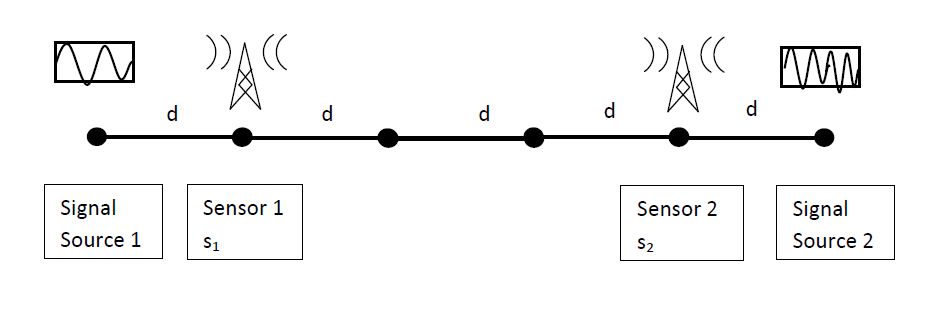
Figure 7. Transmitters and receivers

This situation describes a separable sensing scenario since the received signal level on each frequency at each receiver is given as the transmitted power, $\alpha_{1}$ and $\alpha_{2},$ respectively, multiplied by the free space losses, $\gamma_{1}(1),$ $\gamma_{1}(2),$ $\gamma_{2}(1),$ and $\gamma_{2}(2),$ at each receiver. The scenario is radiative if both transmitters are operating. If one of the transmitters is turned off, it ceases to be radiative. It is $j$-dominant for $j=1,2$; in fact, since $N=2,$ it is strongly $j$-dominant. It is also harmonious since both receivers hear both transmitters.

Now consider adding a third transmitter-receiver pair at some great distance and with substantial blocking, e.g., on the other side of a mountain or, for an extreme case, the other side of a continent. Transmitter 3 cannot be received by either of the first two receivers nor can the third receiver hear either of the first two transmitters. The scenario is still separable, although several of the $\gamma_{j}$ will be zero; and still radiative provided all transmitters are turned on. However, it is no longer harmonious since it is $3$-disjoint.

Example 3.19 (SONAR and RADAR: harmony).

The SONAR sensing scenario described in Example 2.2 can be considered harmonious, assuming the area of concern is to the north. Much of the area covered by sensor A is also covered by sensor B, albeit with greater noise problems since some areas will only be covered by endfire beams. We note that this scenario is not harmonious if the area of concern is to the east or west.

The RADAR scenario of Example 2.1 will not be harmonious over the oblong sensing scenario described in Figure 1. We note, however, that partial recovery of information is possible using noisy bins near the edge of coverage.

4. Bases, frames, and multiplicative frames

4.1. Frames

There is an intimate connection between reactive sensing theory and the theory of frames. In this subsection we shall define frames, and state some of their relevant properties. The theory of frames will be used in Section 5 as a natural tool for the analysis of reactive sensing problems. Such problems led to our concept of multiplicative frames defined in Subsection 4.2.

A frame for ${\mathbb{C}}^{d}$ is a sequence, $X=\{x_{h}\}_{h=1}^{D}\subseteq{\mathbb{C}}^{d},$ that spans ${\mathbb{C}}^{d},$ i.e.,

(4) $$\forall\,x\in{\mathbb{C}}^{d},\;\exists\,c_{1},\dots,c_{D}\in{\mathbb{C}}^{d}\;{\rm such\;that}\quad x=\sum_{h=1}^{D}\,c_{h}\,x_{h}.$$

This innocent and elementary property is the basis (sic) for the power of frames, and it belies the power of finite frames in dealing with numerical stability, robust signal representation, and noise reduction problems, see, e.g., [18], [6] Chapters 3 and 7, [14], [25], and [26]. The following definition for Hilbert spaces is equivalent to the definition of frames for ${\mathbb{C}}^{d},$ but is formulated in terms of bounds that are often useful in computation and coding.

Definition 4.1 (Frames).

a. Let ${\mathbb{H}}$ be a separable Hilbert space over the field ${\mathbb{F}}$, where ${\mathbb{F}}={\mathbb{R}}$ or ${\mathbb{F}}={\mathbb{C}},$ e.g., ${\mathbb{H}}=L^{2}({\mathbb{R}}^{d}),{\mathbb{R}}^{d},{\mathbb{C}}^{d}.$ A finite or countably infinite sequence, $X=\{x_{h}\}_{h\in J},$ of elements of ${\mathbb{H}}$ is a frame for ${\mathbb{H}}$ if

(5) $$\exists A,B>0\;\text{such that}\;\forall x\in{\mathbb{H}},\quad A\left\|x\right\|^{2}\leq\sum_{h\in J}|\langle{x},{x_{h}}\rangle|^{2}\leq B\left\|x\right\|^{2}.$$

The optimal constants, viz., the supremum over all such $A$ and infimum over all such $B$, are called the lower and upper frame bounds respectively. When we refer to frame bounds $A$ and $B$, we shall mean these optimal constants. Otherwise, we use the terminology, a lower frame bound or an upper frame bound.

b. A frame $X$ for ${\mathbb{H}}$ is a tight frame if $A=B.$ If a tight frame has the further property that $A=B=1,$ then the frame is a Parseval frame for ${\mathbb{H}}.$

c. A tight frame $X$ for ${\mathbb{H}}$ is a unit norm tight frame if each of the elements of $X$ has norm $1.$ Finite unit norm tight frames for finite dimensional ${\mathbb{H}}$ are designated as FUNTFs.

d. A sequence of elements of ${\mathbb{H}}$, not necessarily a frame, satisfying an upper frame bound, such as $B\left\|x\right\|^{2}$ in (5), is a Bessel sequence.

e. Let ${\mathbb{V}}$ be a vector space over $\mathbb{C}.$ A sequence, $X=\{x_{h}\}_{h=1}^{D}\subseteq{\mathbb{V}}$, is a basis for ${\mathbb{V}}$ if it spans ${\mathbb{V}}$ as in Equation (4) and if $\{x_{h}\}_{h=1}^{D}$ is a linearly independent set, in which case $D$ is the dimension of ${\mathbb{V}}.$ ${\mathbb{V}}$ is infinite dimensional if it contains an infinite linearly independent set. Clearly, if ${\mathbb{V}}$ is a separable Hilbert space, then every basis for ${\mathbb{V}}$ is a frame for ${\mathbb{V}}$.

Let $X=\{x_{h}\}_{h\in J}$ be a frame for ${\mathbb{H}}$. We define the following operators associated with every frame; they are crucial to frame theory. The analysis operator $L:{\mathbb{H}}\rightarrow\ell^{2}(J)$ is defined by

$$\forall x\in{\mathbb{H}},\quad Lx=\{\langle{x,x_{h}}\rangle\}_{h\in J}.$$

The adjoint of the analysis operator is the synthesis operator $L^{\ast}:\ell^{2}(J)\rightarrow{\mathbb{H}}$, and it is defined by

$$\forall a\in\ell^{2}(J),\quad L^{\ast}a=\sum_{h\in J}a_{h}x_{h}.$$

The frame operator is the mapping $\mathcal{F}:{\mathbb{H}}\rightarrow{\mathbb{H}}$ defined as $\mathcal{F}=L^{\ast}L$, i.e.,

$$\forall x\in{\mathbb{H}},\quad\mathcal{F}(x)=\sum_{h\in J}\langle{x,x_{h}}\rangle x_{h}.$$

The following is a fundamental theorem.

Theorem 4.2 (Frame reconstruction formula).

Let ${\mathbb{H}}$ be a separable Hilbert space, and let $X=\{x_{h}\}_{h\in J}\subseteq{\mathbb{H}}$.

a. $X$ is a frame for ${\mathbb{H}}$ with frame bounds $A$ and $B$ if and only if $\mathcal{F}:{\mathbb{H}}\rightarrow{\mathbb{H}}$ is a topological isomorphism with norm bounds $\left\|\mathcal{F}\right\|_{op}\leq B$ and $\left\|\mathcal{F}\right\|_{op}^{-1}\leq A^{-1}$.

b. In the case of either condition of part a, we have the following:

(6) $$B^{-1}I\leq\mathcal{F}^{-1}\leq A^{-1}I,$$

$\{\mathcal{F}^{-1}x_{h}\}$ is a frame for $H$ with frame bounds $B^{-1}$ and $A^{-1}$, and

(7) $$\forall x\in{\mathbb{H}},\quad x=\sum_{h\in J}\langle{x,x_{h}}\rangle\mathcal{F}^{-1}x_{h}=\sum_{h\in J}\langle{x,\mathcal{F}^{-1}x_{h}}\rangle x_{h}=\sum_{h\in J}\langle{x,\mathcal{F}^{-1/2}x_{h}}\rangle\mathcal{F}^{-1/2}x_{h}.$$

For a proof of part a., see [8], pages 100–104.

For part b., let $X=\{x_{h}\}_{h\in J}$ be a frame for $H$. Then, the frame operator $\mathcal{F}$ is invertible ([18], [3]); and $\mathcal{F}$ is a multiple of the identity precisely when $X$ is a tight frame. Further, $\mathcal{F}^{-1}$ is a positive self-adjoint operator and has a square root $\mathcal{F}^{-1/2}$ (Theorem 12.33 in [35]). This square root can be written as a power series in $\mathcal{F}^{-1}$; consequently, it commutes with every operator that commutes with $\mathcal{F}^{-1},$ and, in particular, with $\mathcal{F}.$ These properties allow us to assert that $\{\mathcal{F}^{-1/2}\,x_{h}\}$ is a Parseval frame for ${\mathbb{H}}$, and give the third equality of (7). see [14], page 155.

Remark 4.3 (Frames and bases for ${\mathbb{C}}^{d}$ and ${\mathbb{H}}$).

In light of the fact that orthonormal bases (ONBs) are frames, it is natural to ask to what extent frames can be constructed in terms of ONBs. This is pertinent because of our frame results in Section 5 and our simulation in Section 6.

• It may be considered surprising that any infinite dimensional ${\mathbb{H}}$ contains a frame for ${\mathbb{H}}$ which does not contain a basis for ${\mathbb{H}}$. The result is due to Casazza and Christensen, see [14], Chapter 7, for details.

• The first result relating frames and sums of bases is due to Casazza [12]. Let ${\mathbb{H}}$ be a separable Hilbert space over the field ${\mathbb{F}}$, and let $X=\{x_{h}\}_{h\in J}$ be a frame for ${\mathbb{H}}$ with upper frame bound $B$. Then, for every $\epsilon>0$, there are ONBs $\{u_{h}\}_{h\in J},\{v_{h}\}_{h\in J},\{w_{h}\}_{h\in J}$ for ${\mathbb{H}}$ and a constant $C=B(1+\epsilon)$ such that

  $$\forall h\in J,\quad x_{h}=C(u_{h}+v_{h}+w_{h}).$$

  The proof depends on an operator-theoretic argument.

4.2. Multiplicative frames

Because of the formulation described in Section 3, we define the notion of a multiplicative frame.

Definition 4.4 (Multiplicative frames).

A sequence, $X=\{x_{j,k}\}\subseteq{\mathbb{C}}^{n},1\leq j\leq N,1\leq k\leq K$ is a multiplicative frame for ${\mathbb{C}}^{n}$ if it is a frame for ${\mathbb{C}}^{n}$ and if

$$\exists\,\{y_{j}:1\leq j\leq N\}\subseteq{\mathbb{C}}^{n}\>\text{ and }\>\exists\,\{z_{k}:1\leq k\leq K\}\subseteq{\mathbb{C}}^{n}\quad\text{ such that }$$

$$\forall\,j=1,\ldots,N,\,\forall\,k=1,\ldots,K,\>\text{ and }\forall\,i=1,\ldots,n,\quad x_{j,k}(i)=y_{j}(i)\,z_{k}(i).$$

In the following constructions of multiplicative frames, it is important to note that they require the hypotheses of radiativity and dominance given in Definition 3.8. In fact, radiativity is manifested by (8) and dominance is manifested by (9) in Theorem 4.5. Besides Corollary 4.6, this should also be compared with Theorem 5.12. We view this as a striking connection between the mathematical concept of a multiplicative frame and the notions of radiativity and dominance that arise from our physical modeling of a sensing scenario.

Theorem 4.5 (A construction of multiplicative frames).

Given $Y=\{y_{j}:1\leq j\leq N\}\subseteq{\mathbb{C}}^{n}\setminus{\{0\}}\>\text{ and }\>Z=\{z_{k}:1\leq k\leq K\}\subseteq{\mathbb{C}}^{n}\setminus{\{0\}}$, and define $X=\{x_{j,k}:x_{j,k}(i)=y_{j}(i)\,z_{k}(i)\}\subseteq{\mathbb{C}}^{n},1\leq j\leq N,1\leq k\leq K,1\leq i\leq n$.

a. Let $Y$ be a frame for ${\mathbb{C}}^{n}$ with frame constants $A_{N}$ and $B_{N}$, and assume

(8) $$\exists\,k\in\{1,\ldots,K\}\;{\rm such\,that}\;{\rm min}_{1\leq i\leq n}\,|z_{k}(i)|=m_{z}>0.$$

Then, $X$ is a multiplicative frame for ${\mathbb{C}}^{n}$; and an upper frame bound B and a lower frame bound A are constructed in the proof.

b. Let $Z$ be a frame for ${\mathbb{C}}^{n}$ with frame constants $A_{K}$ and $B_{K}$, and assume

(9) $$\exists\,j\in\{1,\ldots,N\}\;{\rm such\,that}\;{\rm min}_{1\leq i\leq n}\,|y_{j}(i)|=m_{y}>0.$$

Then, $X$ is a multiplicative frame for ${\mathbb{C}}^{n}$; and an upper frame bound B and a lower frame bound A are constructed in the proof.

Proof.

a. First, ${\rm card}\,\{x_{j,k}\}=NK$. By the multiplicative definition of each $x_{j,k}$, it is sufficient to prove that $X$ is a frame for ${\mathbb{C}}^{n}$.

Let $x=(x(1),x(2),\ldots,x(n))\in{\mathbb{C}}^{n}$. Then,

$$\sum_{j=1,\ldots,N,\,k=1,\dots,K}\,|\langle x,x_{j,k}\rangle|^{2}=\sum_{k=1}^{K}\sum_{j=1}^{N}\,|\langle x,x_{j,k}\rangle|^{2}=\sum_{k=1}^{K}\sum_{j=1}^{N}\,|\langle x,y_{j}z_{k}\rangle|^{2}$$

$$=\sum_{k=1}^{K}\sum_{j=1}^{N}\,|\langle x\overline{z}_{k},y_{j}\rangle|^{2}=\sum_{k=1}^{K}\sum_{j=1}^{N}\,\left|\sum_{i=1}^{n}\,x(i)\overline{z_{k}(i)}\,\overline{y_{j}(i)}\right|^{2}.$$

Thus, since

$$\sum_{k=1}^{K}\sum_{j=1}^{N}\,|\langle x,x_{j,k}\rangle|^{2}=\sum_{k=1}^{K}\,\sum_{j=1}^{N}\,|\langle x\overline{z}_{k},y_{j}\rangle|^{2},$$

we have

(10) $$\sum_{k=1}^{K}\,A_{N}\,\|x\overline{z}_{k}\|_{2}^{2}\leq\sum_{k=1}^{K}\,\sum_{j=1}^{N}\,|\langle x,x_{j,k}\rangle|^{2}\leq\sum_{k=1}^{K}\,B_{N}\,\|x\overline{z}_{k}\|_{2}^{2}.$$

Next, we make the estimate,

(11) $$\sum_{k=1}^{K}\,\|x\overline{z}_{k}\|_{2}^{2}=\sum_{k=1}^{K}\,\left(\sum_{i=1}^{n}\,|x(i)|^{2}|\overline{z_{k}(i)}|^{2}\right)$$

$$\leq\sum_{k=1}^{K}\,{\rm max}_{1\leq i\leq n}\,|z_{k}(i)|^{2}\,\left(\sum_{i=1}^{n}\,|x(i)|^{2}\right)$$

$$=\|x\|_{2}^{2}\,\sum_{k=1}^{K}\,\|z_{k}\|_{\infty}^{2}\leq K\,\left({\rm max}_{1\leq k\leq K}\,\|z_{k}\|_{\infty}^{2}\right)\,\|x\|_{2}^{2}.$$

Therefore,

$$\sum_{j=1,\ldots,N,\,k=1,\dots,K}\,|\langle x,x_{j,k}\rangle|^{2}\leq K\,B_{N}\,\left({\rm max}_{1\leq k\leq K}\,\|z_{k}\|_{\infty}^{2}\right)\,\|x\|_{2}^{2}.$$

Consequently, and only assuming that $\{y_{j}\}$ is a Bessel sequence with Bessel bound $B_{N}$, we obtain that $\{x_{j,k}\}$ is a Bessel sequence for ${\mathbb{C}}^{n}$ with Bessel bound, and an upper frame bound, $K\,B_{N}\,\left({\rm max}_{1\leq k\leq K}\,\|z_{k}\|_{\infty}^{2}\right)$.

Finally, to obtain a lower frame bound, we proceed as follows. We combine (10) and (11) with the hypothesis, (8), to make the estimate,

$$\sum_{k=1}^{K}\,A_{N}\,\|x\overline{z}_{k}\|_{2}^{2}\geq m_{z}\,A_{N}\,\|x\|_{2}^{2}.$$

In particular, a lower frame bound is $m_{z}\,A_{N}$.

b. The proof of part b is analogous to that of part a with the roles of $Y$ and $Z$ reversed. ∎

We state Corollary 4.6 as a corollary of Theorem 4.5. In fact, since none of the elements of $Y$ or $Z$ is the $0$-vector, conditions (8) and (9) are automatically satisfied.

Corollary 4.6 (A construction of multiplicative frames for two frames).

Let $Y=\{y_{j}:1\leq j\leq N\}\subseteq{\mathbb{C}}^{n}\setminus\{0\}\>\text{ and }\>Z=\{z_{k}:1\leq k\leq K\}\subseteq{\mathbb{C}}^{n}\setminus\{0\}$ be frames for ${\mathbb{C}}^{n}$ Then, $X=\{x_{j,k}:x_{j,k}(i)=y_{j}(i)\,z_{k}(i)\}\subseteq{\mathbb{C}}^{n},1\leq j\leq N,1\leq k\leq K,1\leq i\leq n$ is a multiplicative frame for ${\mathbb{C}}^{n}.$

In our forthcoming theory of multiplicative frames we would need to evaluate more refined frame bounds for results such as Theorem 4.5 and Corollary 4.6.

Our intention is to connect the notion of a separable sensing scenario to the theory of frames. In Section 5.1 we shall start with a separable sensing scenario and use the health space mapping $H$ to construct basis and frame mappings from sets $\{v_{j,k}\}$ of sensor data into ${\mathbb{C}}^{n},$ where $j$ indicates one of the $N$ sensors, $k$ designates one of the $K$ times, and each $v_{j,k}$ is evaluated at some $f\in\{1,\ldots,M\}.$ In some cases, these mappings will give rise to multiplicative bases for ${\mathbb{C}}^{n},$ while in other cases they will give rise to multiplicative frames. The former will be called basis mappings, while the latter will be called frame mappings, as defined in Subsection 5.1.

5. Reactive sensing theory

5.1. Basis and frame mappings

Consider a separable sensing scenario $S$ with health space ${\mathbb{C}}^{n}$ and health space mapping $H:{\mathbb{C}}^{M}\longrightarrow{\mathbb{C}}^{n}$. We wish to analyze the state of $S$. At time $k,1\leq k\leq K,$ each sensor $s_{j},1\leq j\leq N,$ generates a vector $v_{j,k}\in{\mathbb{C}}^{M}$, see the beginning of Subsection 3.1 for notation. We use $H$ to map the $v_{j,k}$ to $H(v_{j,k})\in{\mathbb{C}}^{n}.$ Then, generally, we shall have some detection and/or classification scheme in place in ${\mathbb{C}}^{n},$ that allows us to say something about the state of $S$ given the information $H(v_{j,k})\in{\mathbb{C}}^{n}$, see Subsection 6.1.

For example, in the DFT Example 3.3 and later in Section 6, it may be the case that if a particular coordinate $H(v_{j,k})(i)$ is greater than some known value, then a gear fault is indicated.

Remark 5.1 (The role of frames).

One issue that arises immediately is that for a fixed $i\in\{1,\ldots,n\},$ there could be many $H(v_{j,k})(i)$ values from which to choose at time $k$. In fact, we may have one such value for each $j$, $1\leq j\leq N;$ and $N$ could be large. There are applications where a solution may require deploying hundreds of inexpensive sensors, see, e.g., [27], [40], [9].

It is this overdetermined nature of reactive sensing problems that led us to use the theory of frames. In particular, we note that frames are over-complete sets of atoms, as opposed to bases, where the loss of just one basis element can permanently and adversely affect accurate signal representation in terms of the remaining elements of the basis. In this regard, and considering the first signal reconstruction equality of Equation (7) in Section 4, the fact that the $x_{h}$ may form an over-complete set of atoms raises the possibility that the $NK$ vectors $H(v_{j,k})\in{\mathbb{C}}^{n}$ could be a frame for ${\mathbb{C}}^{n},$ see Theorems 5.5 and 5.12.

We now define frame and basis mappings in terms of the mathematical model of Section 3. To set the stage, we consider simultaneously all of the sensor output values in ${\mathbb{C}}^{MN}$ at a fixed time $k,\,1\leq k\leq K$. Our frame and basis mappings are the means of transferring this data to health space, ${\mathbb{C}}^{n}$, where $n$ should typically be less than $MN$. Recall that

$${\rm card}\,\{v_{j,k}\}=KN,\quad{\rm card}\,(S)=M,\quad{\rm and}\quad S=\bigcup_{j=1}^{N}T_{j}.$$

Formally, we define the set,

(12) $$V=\{v_{1,k}\oplus v_{2,k}\oplus\ldots\oplus v_{N,k}:k=1\leq k\leq K\}\subseteq{\mathbb{C}}^{MN},\quad{\rm card}\,(V)=K,$$

consisting of the $K$ $MN-$tuples, $(v_{1,k}(f_{1}),\ldots,v_{1,k}(f_{M}),\ldots,v_{N,k}(f_{1}),\ldots,v_{N,k}(f_{M})),$ and we define the mapping,

$${\mathcal{H}}:{\mathbb{C}}^{MN}\longrightarrow{\mathbb{C}}^{nN},$$

by applying $H$ to each appropriate copy of ${\mathbb{C}}^{M}$ in ${\mathbb{C}}^{MN}$ so that

$${\mathcal{H}}(v_{1,k}\oplus v_{2,k}\oplus\ldots\oplus v_{N,k})=H(v_{1,k})\oplus H(v_{2,k})\oplus\ldots\oplus H(v_{N,k})\in{\mathbb{C}}^{nN}.$$

As noted in Subsection 1.3, Definition 5.2b is technical, and necessarily so in order to obtain the effective quantitative results of Section 6. However, it really only reflects a computational means for using the over-completeness inherent in frames. Definition 5.2a is also technical, and is an analogue for bases in order to compare the roles of bases and frames in reactive sensing implementations.

Definition 5.2 (Basis and frame mappings).

Let $S$ be a separable sensing scenario with health space mapping $H$.

a.i. The first way to describe the state of $S$ at a fixed time, $k,\,k=1,\ldots,K$, is to analyze the values assigned to parameters in $S_{j}$ by sensors $s_{j},$ that bear primary responsibility for those parameters at time $k$, see the beginning of Subsection 3.1. This method will ignore the values assigned to $T_{j}\diagdown S_{j}$ by sensor $s_{j},$ and now allows us to define a mapping,

(13) $$v_{j,k}\mapsto u_{j,k},$$

where $v_{j,k}\in{\mathbb{C}}^{M}$ and $u_{j,k}\in{\mathbb{C}}^{n}$, and where we shall give precise meaning to $u_{j,k}$ for a given $v_{j,k}$.

a.ii. To this end, we begin with a separable sensing scenario $S$ and the sets $I_{j}$ defined in Definition 3.12 of Subsection 3.3. Recall that, notationally,

$$\forall i\in\{1,\ldots,n\},\;\exists j=j(i)\in\{1,\ldots,N\},\,n_{j},\,{\rm and}\,\ell\in\{1,\ldots,n_{j}\}\,{\rm such}\,{\rm that}\,i=i_{\ell,j},$$

where $n=n_{1}+\cdots+n_{N}$. We define the basis mapping,

$$B:{\mathbb{C}}^{MN}\longrightarrow{\mathbb{C}}^{n},$$

by the formula

(14) $$B(\bigoplus_{j^{\prime}=1}^{N}c_{j^{\prime}})(i_{\ell,j})=H(c_{j})(i_{\ell,j})\in{\mathbb{C}},$$

where $j\in\{1,\ldots,N\}$, $H(c_{j})\in{\mathbb{C}}^{n}$ by definition of the given health space mapping $H$ associated with $S$, $\ell\in\{1,\ldots,n_{j}\}$, and each $c_{j^{\prime}}\in{\mathbb{C}}^{M}$, $1\leq j^{\prime}\leq N$. Then, if we fix $j\in\{1,\ldots,N\}$ and $k\in\{1,\ldots,K\}$, and set $c_{j^{\prime}}=0\in{\mathbb{C}}^{M}$ for each $j^{\prime}\neq j$, we write

$$B((0,\ldots,0,v_{j,k},0,\ldots,0))=u_{j,k}\in{\mathbb{C}}^{n}.$$

Thus, for each $j\in\{1,\ldots,N\}$ and $k\in\{1,\ldots,K\}$, we have

(15) $$u_{j,k}=\begin{cases}H(v_{j,k})(i)&\text{if}\,i=i_{\ell,j}\,\text{for some}\,\ell\in\{1,\ldots,n_{j}\},\\ 0&\text{if}\,i=i_{\ell,j^{\prime}}\,\text{for all}\,j^{\prime}\neq j.\end{cases}$$

a.iii. As a simple, illustrative example, consider a scenario with two sensors, $s_{1}$ and $s_{2}$, each of which produces a two dimensional vector for each time $k$. Suppose $s_{1}$ bears primary responsibility for the first coordinate, while $s_{2}$ bears primary responsibility for the second. Let us assume $H$ is the identity mapping, so that ${\mathbb{C}}^{M}={\mathbb{C}}^{n}={\mathbb{C}}^{2}$. Suppose at time $k$, $v_{1,k}=(10,2)$ and $v_{2,k}=(-1,7)$. Then, by (15), we have $u_{1,k}=(10,0)$ and $u_{2,k}=(0,7)$. We also have that one element of $V$, defined by Equation (12), will be $(10,2)\oplus(-1,7)\in{\mathbb{C}}^{2\cdot 2}={\mathbb{C}}^{4}$. Applying the mapping $B$ will pick out the first element of the first vector and the second element of the second to form the result: $B((10,2)\oplus(-1,7))=(10,7)$.

a.iv. We note that $B$ naturally decomposes into a composition. In fact, each element of ${\mathbb{C}}^{MN}$ is mapped into its own copy of health space by means of the ${\mathcal{H}}$ mapping, followed by the mapping, $B^{\prime}$, that uses (14) to select the values from each image $H(c_{j})\in{\mathbb{C}}^{n}$ in order to construct the resulting vector. Thus, we write

$$B=B^{\prime}\circ{\mathcal{H}}.$$

b.i. The second way to describe the state of $S$ at a fixed time $k$ is to analyze all of the reported data supplied by all of the sensors. Thus, rather than only selecting data from the sensor that bears primary responsibility for a parameter, we combine the data from all of the sensors. This approach allows us to define a mapping,

(16) $$v_{j,k}\mapsto w_{j,k},$$

where $v_{j,k}\in{\mathbb{C}}^{M}$, and where $w_{j,k}\in{\mathbb{C}}^{n}$ is only necessarily zero for components corresponding to parameters for which $s_{j}$ does not report any values at all. The result of this strategy is to define what we call frame mappings, and we shall give precise meaning to $w_{j,k}$ for a given $v_{j,k}$ in (18).

b.ii. Unlike the situation for basis mappings described in part a.ii, there are many possible frame mappings that can be formulated. For concreteness we shall define one, in particular, that will exhibit properties that are most useful for frame mappings in general. We define the magnitude sum frame mapping,

$$F:{\mathbb{C}}^{MN}\longrightarrow{\mathbb{C}}^{n},$$

by the formula

(17) $$F(\bigoplus_{j^{\prime}=1}^{N}c_{j^{\prime}})(i)=\sum_{j^{\prime}=1}^{N}|H(c_{j^{\prime}})(i)|\in{\mathbb{C}},\quad 1\leq i\leq n,$$

where $j^{\prime}\in\{1,\ldots,N\}$, $H(c_{j^{\prime}})\in{\mathbb{C}}^{n}$ by definition of the given health space mapping $H$ associated with $S$, and each $c_{j^{\prime}}\in{\mathbb{C}}^{M}$, $1\leq j^{\prime}\leq N$. Then, if we fix $j\in\{1,\ldots,N\}$ and $k\in\{1,\ldots,K\}$, and set $c_{j^{\prime}}=0\in{\mathbb{C}}^{M}$ for each $j^{\prime}\neq j$, we write

(18) $$F((0,\ldots,0,v_{j,k},0,\ldots,0))=w_{j,k},\;{\rm where}\,{\rm each}\;0\in{\mathbb{C}}^{M},$$

taking into account that $H(0)=0\in{\mathbb{C}}^{n}$, see Definition 3.1.

Thus, for each $j=1,\ldots,N,\,k=1,\ldots,K$, and $i=1,\dots,n$, and using the fact that $H(0)=0$, we have

(19) $$w_{j,k}(i)=|H(v_{j,k})(i)|.$$

To see this consider the following $N$-tuple of $M$-tuples for (17):

$$c_{j^{\prime}}=0\in{\mathbb{C}}^{M}\;{\rm if}\;j^{\prime}\neq j\quad{\rm and}\quad c_{j^{\prime}}=v_{j,k}\in{\mathbb{C}}^{M}\;{\rm if}\;j^{\prime}=j.$$

Then,

$$F(\bigoplus_{j^{\prime}=1}^{N}c_{j^{\prime}})(i)=|H(v_{j,k})(i)|,$$

and so (19) is obtained by (18).

b.iii. For the numerical example in part a.iii, the mapping, $v_{j,k}\mapsto w_{j,k}$, is simply the magnitude sum frame mapping on the components, and so $w_{1,k}=(10,2)$ and $w_{2,k}=(1,7)$. Evaluating $F$, we compute that $F((10,2)\oplus(-1,7))=(10,2)+(1,7)=(11,9)$.

b.iv. We note that $F$ naturally decomposes into a composition. In fact, each element of ${\mathbb{C}}^{MN}$ is mapped into its own copy of health space by means of the ${\mathcal{H}}$ mapping, followed by the mapping, $F^{\prime}$, that is defined by computing the sum of the magnitudes of the components of each $H(c_{j})\in{\mathbb{C}}^{n}$ in order to construct the resulting vector, see (17). Thus, we write

$$F=F^{\prime}\circ{\mathcal{H}}.$$

c. The basis mapping $B$ is linear and the magnitude sum frame mapping $F$ is non-linear, although it could be linear on subspaces. In general, linearity is neither necessarily natural nor desirable for some realistic sensing scenarios. For example, if the signal to noise ratio (SNR) of data reported by different sensors varies, it may make sense to scale data non-linearly before performing the addition in the frame mapping $F$, see Subsection 6.6.

Remark 5.3 (A non-commutative diagram).

There is the following natural non-commutative diagram, Figure 8, associated with Definition 5.2.

$$\begin{CD}V\subset{\mathbb{C}}^{MN}@>{\mathcal{H}}>{}>{\mathbb{C}}^{nN}\\ @V{}V{\mathcal{H}}V@V{}V{B^{\prime}}V\\ {\mathbb{C}}^{nN}@>{F^{\prime}}>{}>{\mathbb{C}}^{n}\end{CD}$$

Figure 8. Non-commutative diagram

In order to illustrate the two flows, basis and frame, in Figure 8 and the precise definition of both $B^{\prime}\circ{\mathcal{H}}$ and $F^{\prime}\circ{\mathcal{H}}$, recall that $\{I_{j}\}$ (Definition 3.12) is a partition of $\{1,\ldots,n\}$ and that some of the $I_{j}$ could be empty. Thus, if $i\in\{1,\ldots,n\}$, then $i$ is in a unique $I_{j}$ and there is a unique $\ell\in\{1,\ldots,n_{j}\}$ such that $i=i_{\ell,j}$, see (2) and (3). Also, from the definition of ${\mathcal{H}}$ we have

$${\mathcal{H}}(v_{k})=H(v_{1,k})\oplus H(v_{2,k})\oplus\ldots\oplus H(v_{N,k})\in{\mathbb{C}}^{nN},$$

where $v_{k}=v_{1,k}\oplus v_{2,k}\oplus\ldots\oplus v_{N,k}\in V$.

Thus, for the case of basis mappings and for a fixed $i\in\{1,\ldots,n\}$, we compute for any $k$, that

$$B^{\prime}\circ{\mathcal{H}}(v_{k})(i)=H(v_{j,k})(i_{\ell,j})\in{\mathbb{C}},$$

where $j$ and $\ell$ are specified by the initial choice of $i$. Similarly, for the case of magnitude sum frame mappings and for a fixed $i\in\{1,\ldots,n\}$, we compute for any $k$, that

$$F^{\prime}\circ{\mathcal{H}}(v_{k})(i)=\sum_{j^{\prime}=1}^{N}|H(v_{j,k})(i_{\ell,j})|\in{\mathbb{C}}.$$

For the example of Definition 5.2 a.iii, b.iii, we note that

$$B^{\prime}\circ{\mathcal{H}}\,((10,2)\oplus(-1,7)=(10,7),$$

and

$$F^{\prime}\circ{\mathcal{H}}\,((10,2)\oplus(-1,7)=(11,9).$$

Remark 5.4 (An advantage of frame mappings).

Specific basis and frame mappings, $B$ and $F$, can be constructed depending on the application. In fact, the complexity of the mappings, $B$ and $F$, can be expected to be data and/or problem dependent, and there are many possible definitions. However, in all cases, we want to distinguish quantitatively between the singular role of a single sensor or small group of sensors associated with a component of a sensing scenario (the mappings $B$) and the impact of all of the sensors (the mappings $F$) to deal with the case that a particular sensor or group of sensors might be disabled.

An advantage of a frame mapping is that in the event of the loss of one or more sensors, some of the missing data can be recovered. For example, suppose $s_{j}$ bears primary responsibility for a parameter $f$. As formulated in Remarks 3.9b and 3.15a, suppose there is an $i\in I_{j}$ associated with $f$. If sensor $s_{j}$ becomes non-operational, then the basis mapping vectors $u_{j,k}$ are all $0$. Further, by the formulation of a basis mapping, all of the other basis mapping vectors, $u_{j^{\prime},k},\,j^{\prime}\neq j$, will have the property that $u_{j^{\prime},k}(i)=0$. Thus, all vectors in the image of the basis mapping will have their $i$-th component equal to $0$; and hence vital information has been lost. However, for the frame mapping, there may be a vector $w_{j^{\prime},k},\,j^{\prime}\neq j$ for which $w_{j^{\prime},k}(i)\neq 0$. This will be the case, in particular, when the scenario is $j$-harmonious. We shall explore this phenomenon in Subsection 5.2.

5.2. Fundamental theorems

In this subsection we prove the main results of reactive sensing theory. We shall show that if a basis mapping is applied to an appropriate set, then it will generate a basis, and if a frame mapping is applied to the same set, then it will generate a frame. These facts are essential in order for our mathematical model to distinguish between sensor failure and critical sensed events.

For the basic set-up, consider the set $V$, which contains the $K$ vectors, $v_{1,k}\oplus\ldots\oplus v_{j,k}\oplus\ldots\oplus v_{N,k}\in V\subseteq{\mathbb{C}}^{MN},\,1\leq k\leq K$. Each $v_{j,k}$ is mapped by $H$ to $H(v_{j,k})\in{\mathbb{C}}^{n}.$ Using the notation from Subsection 5.1, we write ${\mathcal{H}}:V\rightarrow{\mathbb{C}}^{nN}$ evaluated at $v_{1,k}\oplus\ldots\oplus v_{j,k}\oplus\ldots\oplus v_{N,k}$ as

$${\mathcal{H}}(v_{1,k}\oplus\ldots\oplus v_{j,k}\oplus\ldots\oplus v_{N,k})=(H(v_{1,j}),...,H(v_{j,k}),...,H(v_{N,k}))\in{\mathbb{C}}^{nN},$$

where each $H(v_{j,k})$ is a vector of the form,

$$(H(v_{j,k})(1),...,H(v_{j,k})(i),...,H(v_{j,k})(n))\in{\mathbb{C}}^{n}.$$

We now look at the individual components for the image vectors under this mapping. Specifically, we define the projective set $X$ as

(20) $$X=\{(0,...,0,H(v_{j,k})(i),0,...,0)\in{\mathbb{C}}^{n}:1\leq i\leq n,\ 1\leq j\leq N,\ 1\leq k\leq K\},$$

where $H(v_{j,k})(i)$ is the $i$-th component of the vector $H(v_{j,k})$ in ${\mathbb{C}}^{n}.$ Note that ${\rm card}\,X=nNK$.

Theorem 5.5 (Conditions for projective multiplicative frames).

Let $S$ be a separable sensing scenario with partition $\{S_{j}\}_{j=0}^{N},$ covering $\{T_{j}\}_{j=1}^{N},$ and mappings $s_{j}:T_{j}\times\{1,\ldots,K\}\rightarrow{\mathbb{C}}^{M}$, where $s_{j}(f,k)=v_{j,k}(f)$ for $f\in T_{j}$ and $v_{j,k}(f)=0$ for $f\in S\backslash T_{j}.$ Let $H:{\mathbb{C}}^{M}\rightarrow{\mathbb{C}}^{n}$ be a health space mapping of the form,

$$\forall\,j=1,\ldots,N\;{\rm and}\;\forall\,k=1,\ldots,K,\quad H(v_{j,k})(i)={\gamma}_{j}(i)\,{\alpha}_{k}(i),$$

where $i=1,\ldots,n.$ If $S$ is $i-$radiative and $i-$dominant for each $i=1,\ldots,n,$ then $X\subseteq{\mathbb{C}}^{n},$ defined by Equation (20), is a multiplicative frame for ${\mathbb{C}}^{n}.$

Proof.

Take any $i\in\{1,...,n\},$ noting it is of the form $i=i_{\ell,j}$ for some $j\in\{1,...,N\}$ and some $\ell\in\{1,...,n_{j}\}$, see Definition 3.12.

From radiativity, for $i=i_{\ell,j},$ there is $k_{i}$ such that $\alpha_{k_{i}}(i)\neq 0$. Since $i=i_{\ell,j}$ and $s_{j}$ is $i$-dominant, we have $\gamma_{j}(i_{\ell,j})\neq 0.$ Therefore, $H(v_{j,k_{i}})(i_{\ell,j})\neq 0$. Consequently,

$$(0,\dots,0,H(v_{j,k_{i}})(i),0,\dots,0)\in X\subseteq{\mathbb{C}}^{n}$$

is not the zero vector. Hence, the $n$ vectors we obtain, one for each $i,$ form a basis for ${\mathbb{C}}^{n}$ and the result is proved. ∎

Theorem 5.6 (Harmonious multiplicative frames).

Let $S$ be a separable sensing scenario as described in Theorem 5.5. Assume $S$ is $i-$radiative and $i-$dominant for each $i=1,\ldots,n$, and assume $S$ is $j$-harmonious. If sensor $s_{j}$ fails and becomes non-operational, then $X\subseteq{\mathbb{C}}^{n}$ is still a multiplicative frame for ${\mathbb{C}}^{n}.$

Proof.

Fix $j$. Since $s_{j}$ is non-operational we have that

$$\exists\ell\in\{1,\ldots,n_{j}\}\neq\emptyset\quad\text{such that}\quad\gamma_{j}(i_{\ell,j})=0.$$

Then, as before,

$$\forall i=i_{\ell,j^{\prime}},\ \ell\in\{1,...,n_{j^{\prime}}\},\ j^{\prime}\neq j,\quad(0,\dots,0,H(v_{j,k_{i}})(i),0,\dots,0)\neq 0\in{\mathbb{C}}^{n}.$$

This gives $n-n_{j}$ non-zero basis vectors.

For $i=i_{\ell,j},\ \ell\in\{1,...,n_{j}\}$, we may have $\gamma_{j}(i_{\ell,j})=0.$ However, by the $j-$harmonious property,

$$\exists j^{\prime}_{\ell,j}\quad\text{such that}\quad\gamma_{j^{\prime}_{\ell,j}}(i_{\ell,j})\neq 0.$$

From $i$-radiativity, there is $k_{i}\ \text{such that}\ \alpha_{k_{i}}(i_{\ell,j})\neq 0$. Therefore, we have

$$H(v_{j^{\prime}_{\ell,j},k_{i}})(i_{\ell,j})=\gamma_{j^{\prime}_{\ell,j}}(i_{\ell,j})\alpha_{k_{i}}(i_{\ell,j})\neq 0.$$

Thus,

$$(0,...,0,H(v_{j^{\prime}_{\ell,j},k_{i}})(i_{\ell,j}),0,...,0)\neq 0\in{\mathbb{C}}^{n}.$$

This gives the remaining $n_{j}$ non-zero basis vectors, thereby creating a basis in ${\mathbb{C}}^{n},$ and this completes the proof. ∎

We now relate Theorems 5.5 and 5.6 to the basis and frame mappings defined in Subsection 5.1.

As above, $V=\{v_{1,k}\oplus v_{2,k}\oplus...\oplus v_{N,k}:k=1,...,K\}\subseteq{\mathbb{C}}^{MN},$ and we have $B(V)\subseteq{\mathbb{C}}^{n}$ and $F(V)\subseteq{\mathbb{C}}^{n},$ as well as the compositions, $B=B^{\prime}\circ{\mathcal{H}}$ and $F=F^{\prime}\circ{\mathcal{H}}.$ We want to examine the component mappings, $B^{\prime}$ and $F^{\prime}$. To this end we look at the coordinate components of the elements of ${\mathcal{H}}(V)\subseteq{\mathbb{C}}^{nN},$ obtained by projecting each image vector onto its $nN$ coordinates. Thus, for each vector $v\in V,v=v_{1,k}\oplus v_{2,k}\oplus...\oplus v_{N,k}$ for some $k$, we obtain $nN$ projection vectors of the form $(0,0,0...,0,(0,0,...,0,H(v_{j,k})(i),0,...,0),0,...,0)$. Note that the 0s inside only one set of parentheses are the $0\in{\mathbb{C}}^{n}$ vectors, while the 0s in the inner set of parentheses are $0\in{\mathbb{C}}$. Further, the cardinality of the set of all such projection vectors is $nNK$. We wish to look at a subset of these vectors obtained by taking radiativity into account. Assuming we are working with a radiative separable sensing scenario, then, for each $i,\ i=1,...,n$, we can find $k=k_{i}$, such that $\alpha_{k_{i}}(i)\neq 0$. As such, we define

$$Z=\{(0,0,..,0,(0,0,...0,H(v_{j,k_{i}})(i),0,...,0),0...,0),j=1,...,N,\text{ and }i=1,...,n\}\subseteq{\mathbb{C}}^{nN},$$

where, once again, the 0s inside only one set of parentheses are the $0\in{\mathbb{C}}^{n}$ vectors, while the 0s in the inner set of parentheses are $0\in{\mathbb{C}}$. Note that card(Z)=$nN$. We now apply the mappings $B^{\prime}$ and $F^{\prime}$ to the set $Z$.

Theorem 5.7 (Basis mappings and a basis for ${\mathbb{C}}^{n}$).

Let $S$ be a separable sensing scenario as described in Theorem 5.5. Assume that $S$ is $i-$radiative and $i-$dominant for each $i=1,\ldots,n$. The set, $B^{\prime}(Z)$, is the union of a basis for ${\mathbb{C}}^{n}$ and the vector, $0\in{\mathbb{C}}^{n}$.

Proof.

Let $z_{j,i}=(0,...,0,(0,...,0,H(v_{j,k_{i}})(i),0,...,0),0,...,0)$. Then, from the definition of $B$ and $B^{\prime},$ we have $B^{\prime}(z_{j,i})=0\in{\mathbb{C}}^{n}$ unless $i=i_{\ell,j}$. In this case we have $B^{\prime}(z_{j,i})(i^{\prime})=0\in{\mathbb{C}}$ except when $i^{\prime}=i=i_{\ell,j}$. $B^{\prime}(z_{j,i})(i)=\gamma_{j}(i)\alpha_{k_{i}}(i)\neq 0$ since $i=i_{\ell,j}$. This gives precisely $n$ non-zero vectors one for each $i_{\ell,j}$, each a different canonical basis vector. ∎

Corollary 5.8 (Non-operational-sensors and non-bases).

Let $S$ be a separable sensing scenario as described in Theorem 5.5. Assume $S$ is $i-$radiative and $i-$dominant for each $i=1,\ldots,n$. Let $s_{j}$ be a sensor with $n_{j}\neq 0$. If $s_{j}$ is non-operational, then $B^{\prime}(Z)$ will no longer span ${\mathbb{C}}^{n}$ and, hence, will no longer contain a basis.

Proof.

$s_{j}$ non-operational implies there exists an $\ell,\ell\in\{1,\ldots,n_{j}\}\neq\emptyset$ with $\gamma_{j}(i_{\ell,j})=0$. Then, from the proof of Theorem 5.7 the set of $n$ vectors given at the end contains $B^{\prime}(z_{j,i})$ which is of the form $(0,0,0,...,H(v_{j,k})(i),0,...,0)=0\in{\mathbb{C}}^{n}$ since $H(v_{j,k})(i)=\gamma_{j}(i)\,\alpha_{k}(i)=0$. Thus, there cannot be more than $n-1$ non-zero vectors in $B^{\prime}(Z)$ and it cannot span ${\mathbb{C}}^{n}$ ∎

The situation for the frame mapping is more complicated since there can be many possible frame mappings. The next result deals with the magnitude sum frame mapping, but similar results can be obtained for other frame mappings.

Theorem 5.9 (Frame mappings and multiplicative frames for ${\mathbb{C}}^{n}$).

Let $S$ be a separable sensing scenario as described in Theorem 5.5. Assume $S$ is $i-$radiative and $i-$dominant for each $i=1,\ldots,n$. Consider the magnitude sum frame mapping, $F$.The set, $F^{\prime}(Z)$, contains a multiplicative frame for ${\mathbb{C}}^{n}$.

Proof.

For each $i=1,\ldots,n$ and each $j=1,\ldots,N$, consider the vector,

$$z_{j,i}=(0,...,0,(0,...,0,H(v_{j,k_{i}})(i),0,...,0),0,...,0)\in Z\subseteq{\mathbb{C}}^{nN},$$

which we can define by the $i$-radiativity. Then, from the definitions of $F$ and $F^{\prime},$ we see that

$$F^{\prime}(z_{j,i})(i^{\prime})=\begin{cases}|\gamma_{j}(i)|\,|\alpha_{k_{i}}(i)|&\text{ if $i^{\prime}=i$,}\\ 0&\text{ otherwise}.\end{cases}$$

Thus, we have

$$F^{\prime}(z_{j,i})=(0,...,0,|H(v_{j,k_{i}})(i)|,0,...,0)=(0,...,0,|\gamma_{j}(i)|\,|\alpha_{k_{i}}(i)|,0,...,0)\in{\mathbb{C}}^{n}.$$

Unlike the basis case, given $j$, $F^{\prime}(z_{j,i})$ may be non-zero even if $i\notin I_{j}$, i.e., even if $i\neq i_{\ell,j}$ for any $1\leq\ell\leq n_{j}$ . However, for each $i$, we do have $i=i_{\ell,j}$ for some $\ell$ and $j$, so in that case $F^{\prime}(z_{j,i})(i)=|\gamma_{j}(i)|\,|\alpha_{k_{i}}(i)|\neq 0$. Thus, for each $i\in 1,\ldots,n$ we have at least one non-zero vector which is only non-zero in the $i$-th position. Choosing one of these vectors for each $i$, we form a basis contained in $F^{\prime}(Z)$ and therefore $F^{\prime}(Z)$ contains a frame. Since this is a separable sensing scenario, the frame vectors satisfy Definition 4.4 and the frame is multiplicative. ∎

Remark 5.10 ($F^{\prime}(Z)$ and $B^{\prime}(Z)$).

We note that $F^{\prime}(Z)$ and $B^{\prime}(Z)$ are different sets. First, ${\rm card}\,B^{\prime}(Z)=n+1$ since $B^{\prime}(Z)$ consists of $n$ basis vectors plus the zero vector. The set, $F^{\prime}(Z)$, on the other hand, may or may not contain the zero vector, since it is possible that $\gamma_{j}(i)\neq 0$ for all $i\in\{1,...,n\}$ and for all $j\in\{1,...,N\}$. However, $F^{\prime}(Z)$ could contain several similar basis vectors depending on how many $j^{\prime}$ have the property that $\gamma_{j^{\prime}}(i_{\ell,j})\neq 0$ for a given $j$. If $\gamma_{j}(i)\neq 0$ for some $i\neq i_{\ell,j}$ and any $\ell$, then there will be duplicate vectors with non-zero $i$-th components. As the following corollary shows, this property turns out to be useful if a sensor fails

Corollary 5.11 (Non-operational sensors and multiplicative frames).

Let $S$ be a separable sensing scenario as described in Theorem 5.5. Assume $S$ is $i-$radiative and $i-$dominant for each $i=1,\ldots,n$; and also assume that $S$ is j-harmonious as in Theorem 5.6. Consider the magnitde sum frame mapping, $F$. Then, even if sensor $s_{j}$ is non-operational, the set, $\{F^{\prime}(Z)\}$, will still contain a multiplicative frame for ${\mathbb{C}}^{n}.$

Proof.

Following the pattern of Theorems 5.6 and 5.9, we let

$$z_{j,i}=(0,...,0,(0,...,0,H(v_{j,k_{i}})(i),0,...,0),0,...,0)$$

for all $j.$ As in Theorem 5.9 we have

$$F^{\prime}(z_{j,i})(i^{\prime})=\begin{cases}|\gamma_{j}(i)|\,|\alpha_{k_{i}}(i)|&\text{ if $i^{\prime}=i$}\\ 0&\text{ otherwise},\end{cases}$$

and

$$F^{\prime}(z_{j,i})=(0,...,0,|H(v_{j,k_{i}})(i)|,0,...,0)=(0,...,0,|\gamma_{j}(i)|\,|\alpha_{k_{i}}(i)|,0,...,0)\in{\mathbb{C}}^{n}.$$

Now, fix a $j$ and assume $s_{j}$ is non-operational. Then,

$$\forall i=i_{\ell,j^{\prime}},\ \ell\in\{1,...,n_{j^{\prime}}\},\ j^{\prime}\neq j,\ \ \ F^{\prime}(z_{j^{\prime},{k_{i}}})\neq 0\in{\mathbb{C}}^{n}$$

as before. This gives $n-n_{j}$ non-zero basis vectors. For $i=i_{\ell,j},\ \ell\in\{1,...,n_{j}\}$ we may have $\gamma_{j}(i_{\ell,j})=0.$ However, by $j$-harmony,

$$\exists j^{\prime}_{\ell,j}\quad{\rm such\,that}\quad\gamma_{j^{\prime}}(i_{\ell,j})\neq 0.$$

Therefore, we have

$$H(v_{j^{\prime}_{\ell,j},k_{i}})(i_{\ell,j})=\gamma_{j^{\prime}}(i_{\ell,j})\alpha_{k_{i}}(i_{\ell,j})\neq 0,$$

and so

$$F^{\prime}(z_{j^{\prime},i})=(0,\ldots,0,|H(v_{j^{\prime}_{\ell,j},k_{i}})(i_{\ell,j})|,0,\ldots,0)\neq 0\in{\mathbb{C}}^{n}.$$

This gives the remaining $n_{j}$ non-zero basis vectors, one for each $i=i_{\ell,j},\,\ell\in\{1,\ldots,n_{j}\}$. Thus, we have constructed a basis for ${\mathbb{C}}^{n},$ in $F^{\prime}(Z)$. Thus, $F^{\prime}(Z)$ contains a frame. Since this is a separable sensing scenario, the frame vectors satisfy Definition 4.4 and the frame is multiplicative. ∎

5.3. A general theorem and constructive technique for multiplicative frames

Theorem 5.12 below should be compared with Theorem 5.5. To this end, recall that the vectors $w_{j,k}\in{\mathbb{C}}^{n}$ are defined as

(21) $$w_{j,k}=F(0,...0,v_{j,k},0,...0),$$

where, for each fixed $k=1,\ldots,K$, $F$ is the magnitude sum frame mapping defined on ${\mathbb{C}}^{MN}$. Because of this, it makes sense to construct multiplicative frames directly from the set $V$ defined in (12) and illustrated in Figure 8. Also, recall that the frame $X$ of Theorem 5.5 has $nNK$ elements, whereas the frame, $\{w_{j,k}\}\subseteq{\mathbb{C}}^{n}$, of Theorem 5.12 has $NK$ elements. Note that we assume $n\leq N$ in Theorem 5.12, cf. Remark 3.2e. This assumption is needed in our proof of Theorem 5.12, but there are examples of sensing scenarios where $\{w_{j,k}\}$forms a frame even when $N<n$.

Theorem 5.12 (Strong dominance and multiplicative frames).

Let $S$ be a separable sensing scenario with partition $\{S_{j}\}_{j=1}^{N},$ covering $\{T_{j}\}_{j=1}^{N},$ and mappings $s_{j}:T_{j}\times\{1,\ldots,K\}\rightarrow{\mathbb{C}}^{M}$, where $s_{j}(f,k)=v_{j,k}(f)$ for $f\in T_{j}$ and $v_{j,k}(f)=0$ for $f\in S\backslash T_{j}.$ Let $H:{\mathbb{C}}^{M}\rightarrow{\mathbb{C}}^{n}$ be a health space mapping of the form,

$$\forall\,j=1,\ldots,N\;{\rm and}\;\forall\,k=1,\ldots,K,\quad H(v_{j,k})(i)={\gamma}_{j}(i)\,{\alpha}_{k}(i),$$

where $i=1,\ldots,n.$ Assume $N>1$ and $n\leq N$. Consider the magnitude sum frame mapping, $F$. If $S$ is $i-$radiative and strongly $i-$dominant for each $i=1,\ldots,n,$ then $\{w_{j,k}:j=1,\ldots,N\,{\rm and}\,k=1,\ldots,K\}\subseteq{\mathbb{C}}^{n}$ defined by $F$ in Equation (21) is a multiplicative frame for ${\mathbb{C}}^{n}.$

Proof.

i. We shall calculate that $\{w_{j,k}:j=1,\ldots,N\;{\rm and}\;k=1,\ldots,K\}$ contains a basis for ${\mathbb{C}}^{n},$ and this proves the result. The calculation is contained in part ii, where we use $i-$radiativity, and in parts iii and iv, where we use strong $i-$dominance to make a basic estimate.

ii. Separability allows us to write $w_{j,k}=\gamma_{j}\alpha_{k},$ where $\gamma_{j},\alpha_{k}\in{\mathbb{C}}^{n}$ for each $j=1,\ldots,N$ and $k=1,\ldots,K$. Clearly, ${\rm card}\{w_{j,k}\}=NK.$

Fix $i\in\{1,\ldots,n\}$. Since $S$ is $i-$radiative, there is a $1\leq k_{i}\leq K$ such that $\alpha_{k_{i}}(i)\neq 0.$ Therefore, we can choose $k_{i}^{\prime}\in\{1,\ldots,K\}$ such that

(22) $$\forall\,k=1,\ldots,K,\quad|\alpha_{k_{i}^{\prime}}(i)|\geq|\alpha_{k}(i)|\quad{\rm and}\quad|{\alpha}_{k_{i}^{{}^{\prime}}}(i)|>0.$$

Equation (22) follows by choosing ${k_{i}^{\prime}},$ among all possible $k_{i},$ that gives the largest value of $|\alpha_{k_{i}}(i)|$.

Taking any $1\leq j\leq N$, we obtain

(23) $$|w_{j,k_{i}^{\prime}}(i)|=|\gamma_{j}(i)||\alpha_{k_{i}^{\prime}}(i)|,$$

and we let $\alpha\equiv{\rm min}_{1\leq i\leq n}|\alpha_{k_{i}}(i)|$. Clearly, $\alpha>0;$ and (23) allows us to assert that

$$\forall\,j=1,\ldots,N\;{\rm and}\;\forall\,i=1,\ldots,n,\quad|w_{j,k_{i}^{\prime}}(i)|\geq\alpha|\gamma_{j}(i)|.$$

iii. We shall prove that $\{\gamma_{j_{i}}\,\alpha_{k_{i}^{\prime}}:i=1,\ldots,n\}$ is a basis for ${\mathbb{C}}^{n}$, using the calculation from part ii.

Take any $i\in\{1,\ldots,n\}$. Then, from $i-$dominance, there is $j_{i}$ such that $\gamma_{j_{i}}(i)\neq 0$; and, hence, by taking the largest such value we can assert that

$$\exists\,j_{i}\;{\rm such}\,{\rm that}\;\forall\ell\neq j_{i}\quad|\gamma_{j_{i}}(i)|\geq|\gamma_{\ell}(i)|.$$

Consider the $n$ vectors, $w_{j_{i},i}=\gamma_{j_{i}}\alpha_{k_{i}^{\prime}}\in{\mathbb{C}}^{n},\,i=1,...,n,$ that is,

$$w_{j_{i},i}=\gamma_{j_{i}}\alpha_{k_{i}^{\prime}}=(\ldots,\gamma_{j_{i}}(h)\alpha_{k_{i}^{\prime}}(h),\ldots)\in{\mathbb{C}}^{n},\;h=1,\ldots,n.$$

Under the stronger assumption of strong $i-$dominance, we can now verify that they form a basis for ${\mathbb{C}}^{n}.$

iv. Let

(24) $$\sum_{i=1}^{n}\,b_{i}\gamma_{j_{i}}\alpha_{k_{i}^{\prime}}=(0,\ldots,0)\in{\mathbb{C}}^{n},$$

where the notation for the sequence, $\{j_{i}\,:\,i=1,\ldots,n\},$ is that used to define strong $i-$dominance. In this situation, whenever Equation (24) is given, we shall show that each $b_{i}$ is $0.$ Thus, we can conclude that $\{\gamma_{j_{i}}\alpha_{k_{i}^{\prime}}\}$ is a basis for ${\mathbb{C}}^{n}.$

Equation (24) can be written as

$$\forall h=1,\ldots,n,\quad\sum_{i=1}^{n}\,b_{i}\gamma_{j_{i}}(h)\alpha_{k_{i}^{\prime}}(h)=0.$$

Thus, for example, when $h=1,$ we have

$$b_{1}\gamma_{j_{1}}(1)\alpha_{k_{1}^{\prime}}(1)+\sum_{i=2}^{n}b_{i}\gamma_{j_{i}}(1)\alpha_{k_{i}^{\prime}}(1)=0.$$

If $b_{1}\neq 0,$ then

$$\gamma_{j_{1}}(1)\alpha_{k_{1}^{\prime}}(1)=-\sum_{i=2}^{n}\,\frac{b_{i}}{b_{1}}\,\gamma_{j_{i}}(1)\alpha_{k_{i}^{\prime}}(1).$$

By $1-$strong dominance, we have $|\gamma_{j_{1}}(1)|\,>\,|\gamma_{j_{i}}(1)|$ for each $i\in\{2,\ldots,n\}$; In particular, $j_{1}\neq j_{i}$. By $1-$radiativity and the definition of $k_{i}^{\prime}$, we have $|\alpha_{k_{1}^{\prime}}(1)|\geq|\alpha_{k_{i}^{\prime}}(1)|$ for each $i\in\{2,\ldots,n\}.$ Consequently, we have the estimate,

$$\left|\sum_{i=2}^{n}\,\frac{b_{i}}{b_{1}}\,\gamma_{j_{i}}(1)\alpha_{k_{i}^{\prime}}(1)\right|\leq\sum_{i=2}^{n}\,\left|\frac{b_{i}}{b_{1}}\right|\,|\gamma_{j_{i}}(1)|\,|\alpha_{k_{i}^{\prime}}(1)|$$

$$<\sum_{i=2}^{n}\,\left|\frac{b_{i}}{b_{1}}\right|\,|\gamma_{j_{1}}(1)|\,|\alpha_{k_{1}^{\prime}}(1)|\leq|\gamma_{j_{1}}(1)|\,|\alpha_{k_{1}^{\prime}}(1)|(n-1)\max_{2\leq i\leq n}\,\left|\frac{b_{i}}{b_{1}}\right|.$$

We can now return directly to our task of proving that if Equation (24) is given, then each $b_{i}$ is $0.$ If this is not true, then let $b_{h}\neq 0,$ and assume $b_{m}$ is the largest such $b_{h}$ in the sense that $|b_{h}|\leq|b_{m}|$ whenever $h\neq m.$ In particular, $b_{m}\neq 0,$ and (24) implies $\sum_{i=1}^{n}b_{i}\gamma_{j_{i}}(m)\alpha_{k_{i}^{\prime}}(m)=0.$ Therefore,

$$|b_{m}\gamma_{j_{m}}(m)\,\alpha_{k_{m}^{\prime}}(m)|=\left|\sum_{i\neq m}\,b_{i}\,\gamma_{j_{i}}(m)\alpha_{k_{i}^{\prime}}(m)\right|$$

$$\leq\sum_{i\neq m}|b_{i}|\,|\gamma_{j_{i}}(m)\alpha_{k_{i}^{\prime}}(m)|<\frac{|b_{m}|}{N-1}\,\sum_{i\neq m}\,|\gamma_{j_{m}}(m)|\,|\alpha_{k_{i}^{\prime}}(m)|,$$

where the last inequality is due to strong $m-$dominance. Hence, we have

$$|\alpha_{k_{m}^{\prime}}(m)|<\frac{1}{N-1}\,\sum_{i\neq m}\,|\alpha_{k_{i}^{\prime}}(m)|\leq\frac{1}{N-1}\,\sum_{i\neq m}\,|\alpha_{k_{m}^{\prime}}(m)|=\frac{n-1}{N-1}\,|\alpha_{k_{m}^{\prime}}(m)|,$$

a contradiction. Here, we use the assumptions that $n\leq N$ and $N>1.$ Thus, $b_{m}=0$ and so $\{\gamma_{j_{i}}\alpha_{k_{i}^{\prime}}\}$ is a basis for ${\mathbb{C}}^{n}.$ ∎

Example 5.13 (A constructive component for Theorem 5.12).

In order to gain insight into the proof of Theorem 5.12, and simultaneously to introduce a linear algebra approach for computational reasons, let us proceed to prove Theorem 5.12 by showing that $\{w_{j,k_{i}^{\prime}}\}\subseteq{\mathbb{C}}^{n}$ spans ${\mathbb{C}}^{n}$, and, hence, that it is a frame for ${\mathbb{C}}^{n}.$ The approach introduces ancillary $N\times n$ matrices, $(c(j,i)),$ that can be used for computation.

i. We begin, as in the proof of Theorem 5.12 by using radiativity to define $\{w_{j,k_{i}^{\prime}}\}$, and note that ${\rm card}\{w_{j,k_{i}^{\prime}}\}=nN\geq n$. Let $W={\rm span}\{w_{j,k_{i}^{\prime}}\}\subseteq{\mathbb{C}}^{n},$ and suppose $W\neq{\mathbb{C}}^{n}.$ Then,

$$\exists\,y\in{\mathbb{C}}^{n}\backslash\{0\}\;{\rm such\;that}\;\forall\,w\in W,\quad\langle y,w\rangle=0.$$

Using the Hahn-Banach theorem our goal is to obtain a contradiction.

Notationally, let $w_{j,k_{i}^{\prime}}\equiv w_{(j,i)}\in{\mathbb{C}}^{n}.$ Hence, we can order the pairs $(j,i)$ from 1 to $nN.$ Instinctively, we would write $w_{(i,j)},$ as well as $c_{(i,j)}$ below, but the $i$ in these cases is dependent on $k$, and this is our way of dealing with the lexicographic order $j,k$.

ii. Now, let

$$y=\sum_{h=1}^{n}y(h)e_{h}\,,\quad e_{h}=(0,....0,1,0,...),$$

where the ”$1$” in the definition of $e_{h}$ appears in the $h$ position. It is critical to note that $e_{h}$ need not be in $W$ or the orthogonal complement of $W$ in ${\mathbb{C}}^{n}.$

Take any $w\in W$ so that

$$w=\sum_{j=1}^{N}\,\sum_{i=1}^{n}\,c(j,i)w_{(j,i)}\in{\mathbb{C}}^{n},$$

since each $w_{(j,i)}\in{\mathbb{C}}^{n}.$ By hypothesis, we have

$$0=\langle w,y\rangle=\sum_{h=1}^{n}\overline{y(h)}\,\langle\sum_{j=1}^{N}\sum_{i=1}^{n}\,c(j,i)w_{(j,i)}\,,\,e_{h}\rangle,$$

and so

$$0=\sum_{h=1}^{n}\overline{y(h)}\sum_{j=1}^{N}\sum_{i=1}^{n}\,c(j,i)\langle w_{(j,i)},e_{h}\rangle=\sum_{h=1}^{n}\overline{y(h)}\sum_{j=1}^{N}\sum_{i=1}^{n}\,c(j,i)(\sum_{l=1}^{n}e_{h}(l)\overline{w_{(j,i)}(l)})$$

$$=\sum_{h=1}^{n}\overline{y(h)}\sum_{j=1}^{N}\sum_{i=1}^{n}\,c(j,i)w_{(j,i)}(h),$$

where

$$w_{(j,i)}(h)=w_{j,k_{i}^{\prime}}(h)=\gamma_{j}(h)\alpha_{k_{i}^{\prime}}(h).$$

Combining these equations, we obtain

(25) $$0=\sum_{h=1}^{n}\overline{y(h)}\sum_{j=1}^{N}\gamma_{j}(h)\sum_{i=1}^{n}c(j,i)\alpha_{k_{i}^{\prime}}(h),$$

where $(y(1),\ldots,y(n))\neq(0,\ldots,0)$ is fixed and $\{c(j,i):j=1,\dots,N\;{\rm and}\;i=1,\dots,n\}$ is any $nN$-tuple.

We can obtain the desired contradiction when we construct an $nN$-tuple $\{c(j,i)\}$ such that the right side of Equation (25) is non-zero. With this contradiction we can then assert that $W={\mathbb{C}}^{n}$ and so $\{w_{(j,i)}\}$ is a frame for ${\mathbb{C}}^{n}.$

iii. We write Equation (25) as

(26) $$0=\sum_{i,j}c(j,i)\left(\sum_{h\in I}\overline{y(h)}\,{\gamma}_{j}(h)\,{\alpha}_{k_{i}^{\prime}}(h)\right),$$

where $I=\{h\in\{1,\ldots,n\}:y(h)\neq 0\}.$ Let $X=\{(j,i):j=1,\ldots,N\;{\rm and}\;i=1,\ldots,n\}$ have the property that

$$\sum_{h\in I}\overline{y(h)}\,{\gamma}_{j}(h)\,{\alpha}_{k_{i}^{\prime}}(h)\equiv d(j,i)\neq 0.$$

iv. If $X\neq\varnothing,$ then set $c(j,i)=\overline{d(j,i)}$ for $(j,i)\in X$ and $c(j,i)=0$ otherwise. Then,

$$0=\sum_{i,j}c(j,i)\left(\sum_{h\in I}\overline{y(h)}\,{\gamma}_{j}(h)\,{\alpha}_{k_{i}^{\prime}}(h)\right)>0,$$

and this contradicts Equation (26). Thus, $W={\mathbb{C}}^{n}.$

v. Now assume $X=\varnothing,$ i.e., assume

$$\forall\;i=1,\ldots,n\;{\rm and}\;\forall\,j=1,\dots,N,\quad\sum_{h\in I}\overline{y(h)}\,\gamma_{j}(h)\,\alpha_{k_{i}^{\prime}}(h)=0.$$

Then, for any $j_{i}\in\{1,\ldots,N\}$ corresponding to $i\in\{1,\ldots,n\},$ we have

(27) $$\forall\,i=1,\ldots,n,\quad\sum_{h\in I}\overline{y(h)}\,\gamma_{j_{i}}(h)\,\alpha_{k_{i}^{\prime}}(h)=0.$$

It is at this point that we go back to the proof of Theorem 5.12, using the hypotheses of strong dominance and the properties of $n$ and $N$, to choose $\{j_{i}:i=1,\dots,n\}$ such that

$$\{\gamma_{j_{i}}\,\alpha_{k_{i}^{\prime}}:i=1,\ldots,n\}\subseteq{\mathbb{C}}^{n}$$

is a basis for ${\mathbb{C}}^{n}.$ Thus, we can conclude from Equation (27) that $y=0\in{\mathbb{C}}^{n},$ and this contradicts our assumption about $y.$ Therefore, $W={\mathbb{C}}^{n}.$

Example 5.14 (An elementary example).

Consider a sensing scenario $S$ with $K=1$ and with three sensors $s_{1},\,s_{2},\,s_{3}$, where $v_{1,1}=(3,1,1),\,v_{2,1}=(1,3,4)$, and $v_{3,1}=(1,1,5)$. Let $H:{\mathbb{C}}^{3}\longrightarrow{\mathbb{C}}^{2}$ be a health-space mapping defined as the projection mapping onto the first two coordinates. Thus, we have $H(v_{1,1})=(3,1),\,H(v_{2,1})=(1,3)$, and $H(v_{3,1})=(1,1)$. We define $\gamma_{1}(1)=3,\,\gamma_{1}(2)=1,\,\gamma_{2}(1)=1,\,\gamma_{2}(2)=3,\,\gamma_{3}(1)=1$, and $\gamma_{3}(2)=1$. We also define $\alpha_{1}(1)=\alpha_{1}(2)=1$. Then, we obtain $H(v_{j,k})(i)=\gamma_{j}(i)\,\alpha_{k}(i)$, for $j=1,\,2,\,3$ and $k=1$; and so $S$ is a separable sensing scenario. Further, $S$ satisfies the criterion for radiativity, since $\alpha_{1}(i)\neq 0$ for $i=1,\,2$. Finally, we can see that $S$ is strongly $i$-dominant for $i=1,\,2$ by defining $j_{1}=1,j_{2}=2$. We now apply Theorem 5.12, and can assert that $\{w_{j,k}:j=1,\,2,\,3\,{\rm and}\,k=1\}=\{(3,1),\,(1,3),\,(1,1)\}$ is a multiplicative frame for ${\mathbb{C}}^{2}$.

6. Data base and DFT turbine simulation

6.1. Detection strategies

Determining the dimension $n$ of health space is critical to obtaining useful algorithms based on this theory. To this end, we can divide problems into two classes depending on whether $n$ is known a priori or a posteriori. Both cases can arise naturally and the theory will be applicable in both cases, but the algorithms for implementation may be different.

a. In the first case, $n$ is known in advance. This will arise in problems where a detection strategy has already been developed. In fact, for a number of engineering problems, detectors already exist for single sensor output. SONAR, RADAR, and machine diagnostic problems all have detectors associated with a single installation or sensor. In the DFT/turbine example of this section, we assume that the existence of engine faults can be determined by looking for certain spectral lines. In problems of this sort, given accurate sensor data from a working sensor, the detector can determine the status of a turbine. This detector maps the output of a single sensor to health space and thus determines $n$. There is dimension reduction when the data from multiple sensors is combined into something the detector can process and also when the detector produces output of lower dimension than the original data stream. Subsections 6.2 - 6.6 deal with this case.

b. The second case arises when a detection strategy is not known in advance. Consider a large collection of data taken by several sensors. For example, each sensor may be recording images or multispectral data, that must be compressed using a dimension reduction technique before being transmitted to a processing center. It is possible that no detector is available for the compressed data stream.

In this case, a machine learning algorithm may be used to determine the state of the situation observed by the sampled data, e.g., see [22] and the remote sensing applications analyzed in [17],[5], [15]. For example, given a set of known positive and negative detection images, an optimal Bayesian detector such as a matched filter or bank of matched filters may be constructed for the compressed data. The output of these filters would then determine health space and the dimension $n$. We also note that matched filters are only one example, but other machine learning techniques may also be used.

6.2. Data base construction

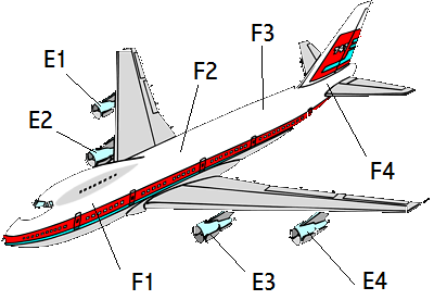
Figure 9. Airplane with engine sensors $E_{j}$ and fuselage sensors $F_{j}$

The theorems and corollaries of Section 5 provide a mathematical framework for the analysis of sensing problems. We now give a detailed example of how this framework applies to a practical simulation for analyzing the DFTs of sensed vibration data. This is, in a way, our canonical situation in that we developed much of the theory of reactive sensing by analyzing the DFT case.

To this end, we now construct a data base to analyze basic vibrations associated with an airplane. We use public domain specification data of major jet engine manufacturers, viz., Boeing, GE, and Pratt-Whitney, see [1], [24], [41]. The engine noise models are simplified since our immediate purpose here is to provide an illustrative sensing scenario, not to solve a complex avionics problem.

Airplane and vibration sensors. In Figure 9, we have an airplane with four engines, $E_{j},\,j=1,2,3,4$, and on each engine there is a vibration sensor $s_{j}$. We also designate sections, $F_{j},\,j=1,2,3,4$, of the fuselage, that may also have sensors attached.

Turbine and gear assumptions. We begin by assuming each engine consists of two turbines spinning at different speeds. Each turbine has fan blades attached to it as well as complex gear assemblies. For simplicity we assume there are only 3 gears in each assembly, one connected to the first turbine and two connected to the second. We assume the basic sounds generated by the engines are spectral lines associated with each of their components. Specifically, each turbine will generate one frequency component at the shaft rotation frequency and another for the blade frequency, which is assumed to be equal to the shaft frequency multiplied by the number of blades. Each of the 3 gears is also assumed to generate a frequency component equal to the gear ratio multiplied by its associated turbine frequency. This gives a total of 7 spectral lines associated with each engine. We assume these spectral lines are unique for each engine. This is a somewhat unrealistic constraint, but it provides an elementary setting in order to evaluate our theory.

Vibration sensor output. So far, we have described the modelling of the engine vibrations themselves. We must now determine what the output of the vibration sensors will be. We assume that the sensor on each engine is primarily responsible for reporting data for that engine, see Subsection 3.1 for the notion of primary responsibility. We also assume that each sensor detects vibrations from the other engines but at a reduced volume. This last assumption is quite natural, but it is significant since it forms the basis for the multiplicative structure developed mathematically in Section 4. Finally, we assume there are noise sources, e.g., air moving across the fuselages, that are also detected by the sensors.

Mixing matrix. To generate the output of the sensors, we define a mixing matrix that determines what proportion of each engine’s vibrations are sensed at each sensor. Specifically, we define a mixing matrix $A=(a_{j,h})$ where each entry $a_{j,h}$ gives the relative volume of engine $E_{h}$ reported by sensor $s_{j}$. For example, we might have $a_{1,1}=1,\ a_{1,2}=0.1,\$ and $a_{1,3}=0.01$, which would mean sensor $s_{1}$ would register engine $E_{1}$ at nominal volume 1, engine $E_{2}$ at 10 dB down from that level, and engine $E_{3}$ a further 10 dB down (20 dB down in all), see [24].

The data base. We choose the engine vibration outputs we wish to combine and apply the mixing matrix to obtain the desired sensor output. For example, to manufacture data for a properly functioning airplane, we take data that models the noise of each properly working engine, and combine these data using the mixing matrix. To manufacture data for a gear fault in $E_{1}$, replace the properly working engine noise data for $E_{1}$ with the gear fault noise and reapply the mixing matrix. In this fashion we can manufacture data for both properly working and faulty engine operation, as sensed by each of the sensors.

The sensor outputs can now be used to generate the data base. The output of each sensor is processed by an 8192 point DFT in blocks giving 4 copies of ${\mathbb{R}}^{8192}$. We wish to map this data from $({\mathbb{R}}^{8192})^{4}$ into a space where the state of the engines can be assessed using an appropriate detector. It is at this stage that we invoke dimension reduction technology, albeit in an elementary way. In fact, we assume that the health of each engine can be estimated based on the magnitude of the 28 relevant spectral lines (7 for each engine). Thus, health space is ${\mathbb{R}}^{28}$. We implement a simple detector, that operates on ${\mathbb{R}}^{28}$ and is capable of distinguishing normal operation, basic engine faults, and catastrophic engine failure. For example, basic faults, such as a missing gear tooth, are registered in terms of large spectral values; while a catastrophic engine failure would be sensed as missing all spectral data from that engine. For more on detectors, and detection and classification strategies, see [38].

6.3. The data base as a sensing scenario

From a mathematical point of view, what we constructed in Subsection 6.2 is a sensing scenario, as defined in Subsection 3.1. In fact, the sensors $s_{j}$ attached to each engine produce spectral lines by repeatedly computing DFTs on the vibration data. Thus, at fixed discrete times $k$, we obtain vectors $v_{j,k}\in{\mathbb{C}}^{M}$ containing frequency information for each sensor $s_{j},j=1,\ldots,N$. Here, $M=8192$ and $\{1,\ldots,M\}$ is the frequency domain of the DFT. Using the data base, we compute the vibration noise coming from each engine, and apply a mixing matrix to compute the sensor outputs. The initial engine vibrations produce frequencies, $f\in\{1,\ldots,M\}$, with varying amplitudes, ${\widehat{\alpha}}_{k}(f)$. These values are generated by the engines, independent of the sensors, and hence the ${\widehat{\alpha}}_{k}$ are independent of $j$. The mixing matrix determines the relative weights that are used to combine the engine vibrations, thus determining the values of ${\widehat{\gamma}}_{j}(f)$ for each spectral line $f$. This mixing is independent of time, and thus does not depend on $k$. Therefore, for each $s_{j}$, we have

$$v_{j,k}(f)={\widehat{\gamma}}_{j}(f){\widehat{\alpha}}_{k}(f),\quad f\in\{1,\ldots,M\}.$$

This means that our sensing scenario is pre-separable as defined in Definition 3.1.

Further, we define an elementary health space mapping,

$$H:{\mathbb{R}}^{8192}\longrightarrow{\mathbb{R}}^{28},$$

by selecting only the coordinates of the 28 relevant spectral components described above. ${\mathbb{R}}^{28}$ will be the associated health space, and this $H$ will be the health space mapping. It is a projection mapping, and is equivalent to PCA under fairly benign assumptions.

We note that $H$ meets the criteria of Proposition 3.6. Specifically, $H$ is the identity mapping on the subspace ${\mathbb{R}}^{28}$ of relevant spectral frequencies, and it is the 0-mapping everywhere else. Since we have shown our scenario is pre-separable, Proposition 3.6 allows us to conclude that we have a separable sensing scenario with health space mapping $H$.

Using the definitions in Subsection 5.1, we can now define basis and frame mappings for the scenario. From a practical point of view, this is a necessary task, since the sensors are each generating a copy of ${\mathbb{R}}^{8192}$, whereas the health space mapping $H$ only operates on one copy. In any case, we require that the basis mapping $B$ and the frame mapping $F$ both map $({\mathbb{R}}^{8192})^{4}$ to health space:

$$B,F:({\mathbb{R}}^{8192})^{4}\longrightarrow{\mathbb{R}}^{28}.$$

The basis mapping $B$ will map the magnitude of each of the 7 spectral lines for $E_{j}$ recorded by $s_{j}$ to one $7$-dimensional subspace of ${\mathbb{R}}^{28}$. $B$ will ignore the rest of the reported data. We shall define the frame mapping $F$ as the sum of the magnitudes of each of the spectral lines as recorded by all the sensors $s_{j}$. Thus, $F$ is the magnitude sum frame mapping defined in Definition 5.2.

Remark 6.1 (Additional sensors).

We note here that there may be additional sensors attached to the airplane, which, for example, might monitor fuselage vibrations. These have not been included in the current data base and analysis, but one can imagine applying reactive sensing theory to these sensors as well. In fact, one envisages tuning such sensors to sense the shape of the broadband noise envelope, and not only processing the sharp spectral lines associated with the engines.

6.4. DFT - turbine simulation

We now use the data base described in Subsections 6.2 and 6.3 to illustrate a practical sensing scenario. We start with the 4 sensors $s_{j}$, which will each hear clearly its engine $E_{j}$, and we assume it will also hear the other engines $E_{\ell},{\ell}\neq j$, at a lower volume, 10dB or more down along with a significant level of noise in the system. The sensors produce spectral output by computing a DFT at each time $k$. Here we use an 8192 point DFT. As described in Subsection 6.3, the sensed outputs of the spectral components from a given sensor at a given time ($v_{j,k}$) is the product of the volume of the components produced by the engines ($\alpha_{k}$) with the sensor’s ability to hear the components ($\gamma_{j}$).

The assumption that a given sensor can hear all of the engines amounts to describing the covering $T_{j}=S$ for each $j=1,\ldots,4$, where S is the frequency spectrum produced by all of the engines. Here, ${\rm card}\,(S)=M=8192$. Note that a sensor $s_{j}$ can be thought of as bearing primary responsibility for the spectral lines produced by the engine $E_{j}$ to which it is attached (once again see Subsection 3.1 about primary responsibility).Further, since every sensor can hear every engine, albeit at a possibly decreased volume, we can assert that the scenario is harmonious as in Definition 3.16.

The magnitudes of the spectral lines give an element of ${\mathbb{R}}^{8192}$ for each sensor. The basis and frame mappings both combine the sensor output to produce a single element of health space, ${\mathbb{R}}^{28}$, which can then be sent to the detector. The detector processes the magnitudes of the 28 significant spectral lines to determine the fault condition of the airplane. We note that this is consistent with the detection strategy described in Subsection 6.1, part a. Specifically, we are assuming that the 28 relevant spectral lines are known, along with the values for the magnitudes of these lines in a working airplane. We can therefore apply the detector to the output of the basis and frame mappings to obtain detection and classification results.

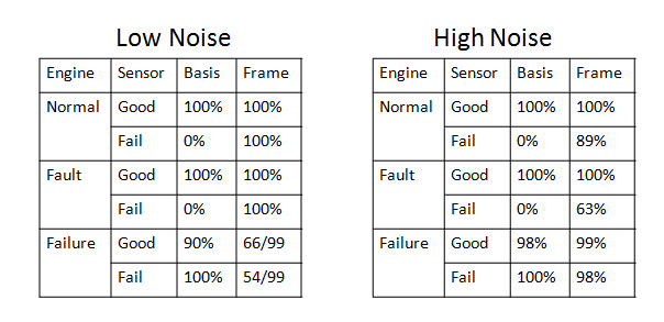
Figure 10. Results

6.5. Results

We now have everything in place to apply the theorems and corollaries of Subsection 5.2. Thus, we can look at the numerical data in Figure 10 to see the relation between these simulated results and the theory. These results were generated by taking samples of data from the database generated in Subsection 6.3. Each sample was processed with an 8192 point DFT. A total of 1024 samples for each of the three different engine states was chosen at random. The three states were the following: normal operation of engine $E_{1}$, gear fault in engine $E_{1}$, and complete failure of engine $E_{1}$.

Figure 10 shows the results of applying the process described in Subsection 6.4 to the data base generated in Subsections 6.2 and 6.3. We consider data from the data base for 12 different conditions: the 3 different engine conditions for $E_{1}$ described above (normal operation, gear fault, and complete engine failure) and 2 different sensor conditions for $s_{1}$ ($s_{1}$ in good operating condition, and $s_{1}$ failure) under the 2 conditions of low background noise and high background noise. For each of these combinations of conditions we report the percentage of correct detections. For the case of complete engine failure in the low background noise environment we report 2 numbers for the frame detector: the first (66 and 54) are strictly engine failure reports, while the second (99 and 99) are combined engine failure and engine fault reports.

The inclusion of additional sensor results in the low noise background tests has caused the frame based approach to confuse fault conditions with failure conditions. Often, multiple fault conditions would be reported.

Good (operational) sensor data from Figure 10. Theorems 5.7 and 5.9 guarantee that the image of certain large sets will form a basis or a frame, respectively, in health space. In either case, we have the ability to span ${\mathbb{R}}^{28}$ and, therefore, our detector should do a good job of classifying the engine condition. Figure 10 shows that when all sensors are operational (Good), normal operation of the engine is correctly identified by both the basis and the frame mappings in both low and high noise environments. This is reflected by the $100\%$ listed in all 4 possible places of the first row of Figure 10. Similarly, both basis and frame processing for operational (Good) sensors correctly identify fault conditions. This is reflected by the $100\%$ listed in all 4 possible places of the third row of Figure 10. The situation is less uniform at identifying engine failure when all sensors are operational (Good). This is the content of the percentages listed in the 4 possible places of the fifth row of Figure 10. When the ambient noise in the system is low, basis processing had a $90\%$ success rate at identifying engine failure. On the other hand, in the same low noise case, the frame mapping sometimes reported an engine fault, or multiple engine faults, when the engine had actually failed. This is reflected by the $66\%$ that is listed. The reason for this is not surprising given the additional noise contributed by the combination of sensors, and the sensitivity of frames in integrating noise into its analysis. The $99\%$ that is listed is the percentage of detecting a fault or engine failure. In the high noise environment, basis and frame processing have an excellent success rate, $98\%$ and $99\%$, respectively, at identifying engine failure when all sensors are operational (Good).

Failed sensor data from Figure 10. The situation is different when a sensor fails. Corollary 5.8 implies that in the case of a basis mapping, there will not necessarily be a corresponding basis in health space; whereas Corollary 5.11 implies that in the case of a frame mapping, there will be a corresponding frame in health space. The results in Figure 10 show that when a sensor fails (Fail), the basis mapping always indicates an engine failure. This is reflected by the two $0\%$ listings in the second row of Figure 10. Of course, sensor failure does not imply engine failure. On the other hand, when a sensor fails, the frame mapping still correctly identifies a normal working engine. This is reflected by the $100\%$ and $89\%$ listings in the second row of Figure 10. Further, when a sensor fails, the frame mapping can still distinguish a normal working engine from a fault or an engine failure, while the basis mapping cannot. This is seen in the fourth line of Figure 10, where the basis mapping reports $0\%$ fault detection while the frame mapping reports $100\%$ in the low noise case and $63\%$ in the high noise case. Of course, the basis mapping will report an engine failure in all cases when the sensor fails, and in the case of an actual engine failure, it will be correct. This is seen in the two $100\%$ entries in the last row. As noted above, the frame mapping has some trouble distinguishing between a fault and an engine failure in the low noise case (the $54\%$ in the bottom row), but does recognize that there is a problem (combined fault and engine failure reports given by the $99\%$ in the bottom row). In the high noise case the frame mapping reports engine failure correctly $98\%$ of the time.

Thus, when a sensor fails, the frame mapping can still give some data about the engine. The basis mapping, however, cannot distinguish between a sensor failure and catastrophic engine failure. In high noise environments, we note that the performance of the frame mapping degrades due to noise, but it is still useful, while the basis mapping is not.

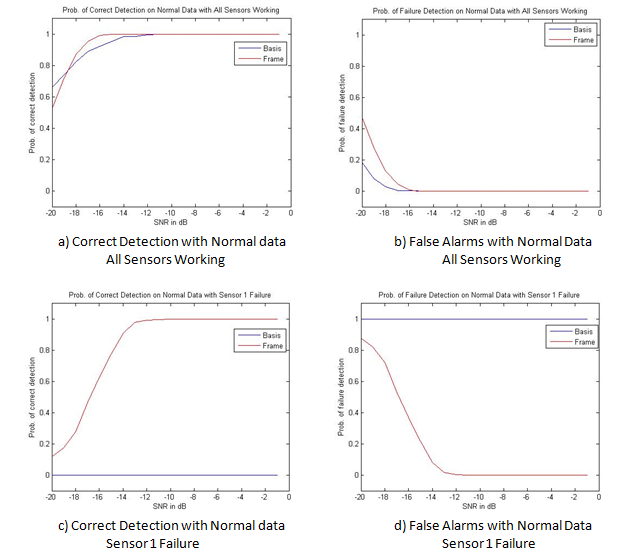
Figure 11. Detection and false alarms

6.6. SNR considerations

The analysis in Subsection 6.5 illustrates some of the features of the frame and basis approaches at a fixed SNR. If we vary the SNR we can gain some insights into the different specific behaviors of each approach. Figure 11 shows what happens to the detector’s ability to determine if there has been a catastrophic failure as the SNR varies from -20 dB to 0 dB.

In each of the four cases in Figure 11 we have assumed all of the engines are working normally. Since the input data is for a properly working engine, all failure and fault detections are false alarms as the result of noise. We only consider statistics for normal engine operation and catastrophic failure. We note that fault detections will count as neither. Further, since all failure and fault detections are the result of noise, we can quantify the performance of each approach as a function of SNR, that is, we can plot the probability of correct detection and the probability of false alarm as functions of SNR in both the cases for properly working sensors and for sensor $s_{1}$ failure. We note that for these results, we have changed the mixing matrix, increasing the levels at which sensor $s_{j}$ will hear engine $E_{\ell}$, for ${\ell}\neq j$, from 10dB down to 5dB. As before we are only looking at results for engine $E_{1}$. Figure 11a shows the correct detections when all sensors are working. When the SNR is high, both the frame and basis approaches give perfect detection, and, as the SNR declines, both show a decline in correct detections. When the SNR falls below -18dB we see that the basis approach has a higher probability than the frame approach of detecting that the engine is performing correctly. This is expected since by looking at other sensors, the frame approach will be forced to contend with additional noise. It is interesting and somewhat counter-intuitive that the frame approach has a higher probability of correct detection between -18 and -12 dB SNR. It turns out that as the noise increases, the basis approach has a greater probability of detecting a fault due to a short term noise spike while the frame approach will average out large noise spikes. However, at low SNR the basis approach detects fewer failures than the frame approach. This can be seen in Figure 11b which shows the false alarms for both approaches. Here it is clear that the elevated noise levels cause the frame approach to report more false alarms.

When sensor $s_{1}$ fails, however, the graphs look significantly different. Figures 11c and 11d show the correct detections and false alarms when sensor $s_{1}$ has failed. Again the data studied is for normal operation, that is, a properly working engine. The frame approach performs well when the SNR is high, giving perfect detection with no false alarms. As the SNR declines we see that for the frame approach, the correct detections decline and the false alarms increase somewhat faster than when sensor $s_{1}$ is working. This is not surprising since effective signal strength is substantially lower without $s_{1}$. The basis approach, however, fails completely as it constantly detects a catastrophic failure regardless of the input data or SNR. This is where the ability of the frame approach to utilize the overdetermined nature of frames comes into play and gives a substantial performance improvement.

7. Epilogue and future

Reactive sensing is an evaluative process to determine the behavior of an object when primary sensor sources of information about the object become unavailable, so that any information must be obtained from the intelligent use of available secondary sensor sources. With regard to a host of applications, e.g., Section 2, loosely connected in terms of machine health, our approach was in terms of physical and mathematical modeling, which in fact interleave and are equivalent.

Our initial, main observation with regard to physical modeling was noting the centrality of combining and relating the volume of a scene and the sensitivity of sensors evaluating that volume, e.g., see Definition 3.1 and Example 3.3 This, in turn, led to the idea of factoring sensor data, and formulating useful notions for this physical modeling, viz., radiative, dominant, and harmonious sensing scenarios, defined in Definitions 3.8 and 3.16 and analyzed throughout Section 3. This factoring of sensor data, coupled with the need to implement our physical modeling led to the development of multiplicative frames, that is the centerpiece of our mathematical modeling. The theory for this development required the content of Section 4.

Reactive sensing, integrating our physical and mathematical modeling, fits naturally into the context of spatial super-resolution. In fact, as noted in Subsection 1.1, the secondary sensor sources can be considered analogous to the role of obtaining a high resolution (HR) image from observed multiple low-resolution (LR) images. In classical super-resolution, the multiple LR images represent different “snapshots” of the same scene, and can be combined to give the desire de facto HR image. In our case, the LR images correspond to secondary sensors and the HR image corresponds to the primary object, that could be disabled or whose primary sensor is not functioning.

Our theory of reactive sensing is given in Section 5. First, we establish the necessity of frames, as opposed to bases, in order to model, both mathematically and effectively, the role of secondary sensor sources, see Subsection 5.1. Then, in Subsection 5.2, we prove the fundamental theorems, that are the basis of our proposed implementation.

Health space ${\mathbb{C}}^{n}$ (Definition 3.1) and dimension reduction are part and parcel of the same idea in reactive sensing with regard to this implementation. In Subsections 6.5 and 6.6, the theory of Section 5 is applied to a DFT turbine simulation.

The experimental results in Section 6 show the efficacy, with some natural qualifications, of frame based reactive sensing theory in detecting engine conditions correctly even in the event of sensor failure. The following are our immediate reactive sensing tasks.

• Apply reactive sensing theory to a spectrum of real data sets, see, e.g., Section 2, and formulate realistic, useful reactive sensing implementations for such sets. This will require more sophisticated dimension reduction technology than PCA, see, e.g., [4].

• Evaluate more deeply the effect of SNR on reactive sensing for scenarios with and without sensor failure. As our simulations have shown, this is a challenging task.

• Develop multiplicative frames as a full-fledged mathematical theory; and especially analyze its relation with frame multiplication theory and group frames, see [2].

8. Acknowledgements

The authors gratefully acknowledge the support of MURI-ARO Grant W911NF-09-1-0383. The first named author also gratefully acknowledges the support of DTRA Grant HDTRA1-13-1-0015, and ARO Grants W911NF-15-1-0112, W911NF-16-1-0008, and W911NF-17-1-0014. This litany of good fortune involved other projects, but also reflects the elephantine gestation period it took for the authors’ original sensor factorization idea to crystalize. Both authors have also benefitted from insightful observations, technical discussions, interest, and support by the following: Drs. David Colella and David Clites (The MITRE Corporation); Kevin Hencke (Systems Engineering Group, Inc. of the Telephonics Corporation, and formerly of the Norbert Wiener Center (NWC)); Tej Phool (MimoCloud); Professors Richard Baraniuk (ECE, Rice University), Alexander Barg (ECE, University of Maryland), Rama Chellapa (ECE, University of Maryland), and Wojciech Czaja (Mathematics, University of Maryland); Drs. Alfredo Nava-Tudela, Matthew Begué (formerly of the NWC), and Celia Rees Evans. Drs. Nava-Tudela and Evans are Scientific Development Officers of the NWC. Finally, we are especially appreciative of the continued confidence of Drs. Liyi Dai, Joseph Myers, and Jay Wilkins Jr.

References

- [1] GE Aviation, Engines 101. http://www.geaviation. com/education/engines101.
- [2] T. Andrews, J. J. Benedetto, and J. J. Donatelli. Frame multiplication theory and a vector-valued dft and ambiguity function. submitted 2917.
- [3] J. J. Benedetto. Frame decompositions, sampling, and uncertainty principle inequalities. In J. J. Benedetto and M. W. Frazier, editors, Wavelets: Mathematics and Applications, pages 247–304. CRC Press, Boca Raton, FL, 1994.
- [4] J. J. Benedetto and W. Czaja. Dimension reduction and remote sensing using modern harmonic analysis. In W. Freeden, Z. Nashed, and T. Sonar, editors, Handbook of Geomathematics, pages 2609–2632. Springer, 2015. Chapter, invited.
- [5] J. J. Benedetto, W. Czaja, J. Dobrosotskaya, T. Doster, and K. Duke. Spatial-spectral operator theoretic methods for hyperspectral image classification. GEM - International Journal on Geomathematics, 7:275–297, 2016.
- [6] J. J. Benedetto and M. Frazier, editors. Wavelets: Mathematics and Applications. Studies in Advanced Mathematics. CRC Press, Boca Raton, FL, 1994.
- [7] J. J. Benedetto and W. Li. Super-resolution by means of Beurling minimal extrapolation. Appl. Comp. Harm. Anlaysis. arXiv:1601.05761, to appear.
- [8] J. J. Benedetto and D. Walnut. Gabor frames for L2 and related spaces. Wavelets: Mathematics and Applications, edited by J.J. Benedetto and M. Frazier, CRC, pages 97–162, 1994.
- [9] R. Boyer. Analysis of the COLD uniform linear array. IEEE 10th Workshop on Signal Processing Advances in Wireless Communications (SPAWC 2009), 2009.
- [10] E. J. Candès and C. Fernandez-Granda. Super-resolution from noisy data. The Journal of Fourier Analysis and Applications, 19(6):1229–1254, 2013.
- [11] E. J. Candès and C. Fernandez-Granda. Towards a mathematical theory of super-resolution. Communications on Pure and Applied Mathematics, LXVII:906–956, 2014.
- [12] P. G. Casazza. Every frame is a sum of three (but not two) orthonormal bases - and other frame representations. J. Fourier Analysis and Applictions, 4(6):727–732, 1998.
- [13] S. Chaudhuri, editor. Super-resolution imaging, chapter 1. SECS 632. Kluwer Academic Publishers, Norwell, Massachusetts 02061 USA, 2001.
- [14] O. Christensen. An Introduction to Frames and Riesz Bases, 2nd edition. Springer-Birkhäuser, New York, 2016 (2003).
- [15] A. Cloninger, W. Czaja, and T. Doster. The pre-image problem for Laplacian eigenmaps utilizing regularization with applications to data fusion. Inverse Problems, to appear.
- [16] H. W. Cole, editor. Understanding Radar. Blackwell Scientific Publications, Amsterdam, 1992.
- [17] W. Czaja, B. Manning, L. McLean, and J. M. Murphy. Fusion of aerial gamma-ray survey and remote sensing data for a deeper understanding of radionuclide fate after radiological incidents: examples from the Fukushima Dai-Ichi response. Journal of Radioanalytical and Nuclear Chemistry, 307:2397–2401.
- [18] I. Daubechies. Ten Lectures on Wavelets. CBMS-NSF Regional Conference Series in Applied Mathematics. Society for Industrial and Applied Mathematics, 1992.
- [19] M. R. Dellomo. Fault detection in helicopter gearboxes using neural networks. J Acoust. Soc., 91 (4):2359, 1992.
- [20] M. R. Dellomo. Helicopter gearbox fault analysis: A neural network approach. ASME Journal of Vibrations and Acoustics, 121(3), July 1999.
- [21] D. L. Donoho. Superresolution via sparsity constraints. SIAM Journal on Mathematical Analysis, 23(5):1309–1331, 1992.
- [22] A. George. Anomaly detection based on machine learning: dimensionality reduction using PCA and classification using SVM. International Journal of Computer Applications, 47, number 21, June 2012, 2012.
- [23] H. Greenspan. Super-resolution in medical imaging. The Computer Journal, 52(1):43–63, 2009.
- [24] K. Hencke. Using a discriminator to improve compressive sesing efficiency. PhD thesis, Norbert Wiener Center, U. of Maryland, College Park, 2012.
- [25] J. Kovačević and A. Chebira. Life beyond bases: The advent of frames (part I). Signal Processing Magazine, IEEE, 24(4):86–104, 2007.
- [26] J. Kovačević and A. Chebira. Life beyond bases: The advent of frames (part II). Signal Processing Magazine, IEEE, 24:115–125, 2007.
- [27] J.-J. Lee, B. Krishnamachari, and C. Kuo. Impact of heterogeneous deployment on lifetime sensing coverage in sensor networks. IEEE Communications Society Conference on Sensor and Ad Hoc Communications and Networks (IEEE SECON), 2004.
- [28] N. Levanon. Radar Principles. John Wiley & Son Inc., 1988.
- [29] N. Levanon and E. Mozeson. Radar Signals. Wiley Interscience, IEEE Press, 2004.
- [30] J. Lindberg. Mathematical concepts of optical superresolution. Journal of Optics, 14(8):083001, 2012.
- [31] S. C. Park, M. K. Park, and M. G. Kang. Super-resolution image reconstruction: a technical overview. IEEE Signal Processing Magazine, pages 21–36, May 2003.
- [32] K. Puschmann and F. Kneer. On super-resolution in astronomical imaging. Astronomy & Astrophysics, 436(1):373–378, 2005.
- [33] T. S. Rappaport. Wireless Communications: Principles and Practice. Dorling Kindersley, 2009.
- [34] M. A. Richards, J. A. Scheer, and W. A. Holm, editors. Principles of Modern Radar. SciTech Publishing, Inc., Raleigh, NC, 2010.
- [35] W. Rudin. Functional Analysis, second edition. McGraw-Hill, 1991 (1973).
- [36] M. I. Skolnik. Introduction to Radar Systems. McGraw-Hill Book Company, New York, 1980.
- [37] G. W. Stimson. Airborne Radar. SciTech Publishing, Inc., Mendham, New Jersey, 1998.
- [38] H. L. V. Trees. Detection, Estimation, and Modulation Theory. Part 4, Optimum Array Processing. Wiley Interscience, New York, NY, 2002.
- [39] J. C. Whitaker. The RF Transmission Systems Handbook, Electronics Handbook Series. CRC Press, Boca Raton, FL, 2002.
- [40] K. Wu, C. Liu, and V. King. Very low cost sensor localization for hostile environments. IEEE International Conference on Communications, 5, 2005.
- [41] J. Yoon. Jet engine types. Aerospaceweb.org – http://www.aerospaceweb.org/question/propulsion/q0033. shtml, 2001.