Minimal Yukawa deflection of AMSB from the Kahler potential

Abstract

We propose a minimal Yukawa deflection scenario of AMSB from the Kahler potential through the Higgs-messenger mixing. Salient features of this scenario are discussed and realistic MSSM spectrum can be obtained. Such a scenario, which are very predictive, can solve the tachyonic slepton problem with less messenger species. Numerical results indicate that the LOSPs predicted by this scenario can not be good DM candidates. So it is desirable to extend this scenario with a Peccei-Quinn sector to solve the strong CP problem and at the same time provide new DM candidates. We propose a way to obtain a light axino mass in SUSY KSVZ axion model with Yukawa deflected anomaly mediation SUSY breaking mechanism. The axino can possibly be the LSP and act as a good DM candidate.

1 Introduction

Low energy supersymmetry(SUSY), which is one of the most attractive extensions of standard model(SM), can solve elegantly the gauge hierarchy problem by introducing various TeV scale superpartners. It can also realize successful gauge coupling unification as well as providing proper dark matter (DM) candidates and baryogensis mechanisms. The Higgs scalar, which was discovered by the ATALS and CMS collaborations of LHC ATLAS:higgs ; CMS:higgs in 2012, lie miraculously in the small ${}^{\prime}115-135^{\prime}$ GeV window predicted by low energy SUSY. Despite of these impressive successes, low energy SUSY confronts many challenges from LHC experiments, especially the null search results of superpartners at LHC which constrain the gluino mass $m_{\tilde{g}}$ to upon 2 TeVCMSSM1 and the top squark mass $m_{\tilde{t}_{1}}$ to upon 1 TeVCMSSM2 in some simplified models. Such difficulties imply that the soft SUSY breaking parameters in low energy SUSY should have an intricate structure.

It is well known that the low energy soft SUSY breaking parameters can be determined by the SUSY breaking mechanism in its UV completed theory. Therefore, it is important to survey which type of SUSY breaking mechanism can accommodate better the phenomenologically favored low energy soft SUSY breaking spectrum, for example, SUGRASUGRA , the gauge mediated SUSY breaking(GMSB)GMSB mechanism or the anomaly mediated SUSY breaking(AMSB)AMSB mechanism. The mSUGRA scenario, which is very predictive, was however disfavored by the global fit of the GAMBIT collaboration even if only the DM relic density upper bound is considered in addition to the muon $g-2$ anomalyGAMBIT . The discovered 125 GeV Higgs boson, which needs a large trilinear coupling $A_{t}$ for TeV scale stop masses, challenges ordinary GMSB scenarios with light stops in which the trilinear couplings are predict to vanish at the messenger scaleGMSB:125 .

Minimal AMSB, which contains only one free parameter $F_{\phi}\simeq m_{3/2}$, is insensitive to the UV theoryAMSB:RGE and predicts a flavor conservation soft SUSY breaking spectrum. Although it is very predictive, minimal AMSB predicts tachyonic slepton masses so that the minimal scenario must be extendedtachyonslepton . The most elegant solution from aesthetical point of view is the deflected AMSBAMSB:deflect ; Nelson:2002sa (dAMSB), in which additional messengers are introduced to deflect the renormalization group equation (RGE) trajectory of AMSB and push the negative slepton squared masses to positive values dAMSB:example . On the other hand, $N\geq 4$ messenger species are always needed to generate positive slepton squared masses with a naturally negative deflection parameter, possibly leading to strong gauge couplings below the GUT scale or Landau pole below the Planck scale. Besides, (radiative) natural SUSY spectrumrnaturalsusy in general is not predicted by ordinary (d)AMSB scenarios. Additional gauge or Yukawa mediation contributions from messenger-matter interactions(mixing) in dAMSB can be advantageous in various aspects. Scenarios with such extensions had been studied in Fei:1508.01299 ; Fei:1602.01699 ; Fei:1703.10894 ; Fei:1704.05079 ; Fei:1710.06105 by one of the authors.

Axion is the pseudo-Goldstone boson associated to the spontaneous breaking of the anomalous Peccei-Quinn(PQ) symmetryPQ that is introduced to solve the ${}^{\prime}strong~{}CP^{\prime}$ problem of QCD. There are two types of popular ${}^{\prime}invisible~{}axion^{\prime}$ model in the literatures, the KSVZ modelKSVZ and the DFSZ modelDFSZ . KSVZ axion model, which can possibly appear in some SUSY breaking mechanisms with a messenger sector, introduces a PQ scalar and additional heavy quarks. Therefore, the induced topological term in its low energy effective theory is the only modification to the standard model Lagrangian. So KSVZ axion model, which predicts no unsuppressed tree-level couplings of axion to standard model matter fields, can evade some of the stringent experimental constraints and is well motivated theoretically. Axino is the fermionic SUSY partner of axion and can act as a cold DM candidatekawasaki . Knowing the axino mass, on the other hand, is essential to determine whether the axino is the LSP or not. In the SUSY extension of KSVZ axion model, the axino mass is always of order $m_{3/2}$ in anomaly mediation scenariosaxino:AMSB and is heavier than ordinary MSSM sparticles. It is therefore interesting to see if the axino can possibly be the LSP and act as the DM particle in anomaly mediation scenarios.

In this paper, we propose to introduce minimal Yukawa deflection by the holomorphic terms in the Kahler potential. Predictive MSSM spectrum can be generated. We also find that the axino can be the LSP through proper Kahler deflection. This paper is organized as follows. In Sec 2, we propose our scenario and discuss the salient features of this scenario. In Sec 3, the soft SUSY parameters are given. The axino mass in an extension of our scenario with a PQ sector is discussed. Our numerical results are given in Sec 4. Sec 5 contains our conclusions.

2 Minimal Yukawa Deflection From Kahler potential

Two approaches are proposed to deflect the AMSB trajectory with the presence of messengers, by pseudo-moduli fieldAMSB:deflect or holomorphic terms (for messengers) in the Kahler potentialNelson:2002sa . Additional Yukawa deflection contributions from messenger-matter interactions(mixing) can also be introduced in both approachesFei:1508.01299 ; Fei:1602.01699 ; Fei:1703.10894 ; Fei:1704.05079 ; Fei:1710.06105 . However, many salient features in scenarioFei:1710.06105 with the Yukawa deflection of the Kahler potential are obscured by the complicate structure of NMSSM. We show that Yukawa deflection from Kaher potential may take the minimal form through Higgs-messenger mixing and its salient features can be seen clearly in this scenario.

We introduce the following holomorphic terms involving the compensator field $\phi$ in the Kahler potential

$$K_{h} \supseteq \phi^{\dagger}\phi\left[c_{1}\bar{X}_{\bf\bar{5}}X_{\bf 5}+c_{2}\bar{H}_{\bf\bar{5}}X_{\bf 5}+c_{3}\bar{X}_{\bf\bar{5}}H_{\bf 5}+c_{4}\bar{H}_{\bf\bar{5}}H_{\bf 5}+\sum\limits_{k=1}^{N_{S}}\kappa_{k}\bar{S}_{k}S_{k}\right]+h.c.~{},$$ (1)

with $\bar{H}_{\bf\bar{5}},H_{\bf 5}$ the Higgs superfields and $X_{\bf 5},\bar{X}_{\bf\bar{5}}$ the messenger superfields in ${\bf 5}$ and ${\bf\overline{5}}$ representations of SU(5), respectively. $\bar{S}_{k},S_{k}$ are respectively the spectator messenger fields in ${\bf\overline{5}}$ and ${\bf 5}$ representations of SU(5), which are introduced to change only the gauge beta functions. Note that $\bar{S}_{k},S_{k}$ cannot be the PQ messengers $Q_{i},\tilde{Q}_{i}$ introduced in KVSZ axion model because the PQ messenger combinations $\tilde{Q}_{i}Q_{i}$ will carry non-trivial PQ charges and cannot appear as holomorphic terms in the Kahler potential.

As any non-singular matrix can be diagonalized by bi-unitary transformations $M_{d}^{\prime}=U^{\dagger}MV$, the previous expressions can be rewritten in the matrix form

$$(\bar{X}_{\bf\bar{5}}~{},\bar{H}_{\bf\bar{5}}) \left(\begin{array}[]{cc}~{}c_{1}{}&~{}c_{2}{}\\ ~{}c_{3}{}&~{}c_{4}{}\end{array}\right)\left(\begin{array}[]{c}X_{\bf 5}\\ H_{\bf 5}\end{array}\right)~{},$$ (6)

$$=(\bar{X}_{\bf\bar{5}}~{},\bar{H}_{\bf\bar{5}})U^{\dagger} \left(\begin{array}[]{cc}~{}c_{a}{}&~{}0{}\\ ~{}0{}&~{}c_{b}{}\end{array}\right)V\left(\begin{array}[]{c}X_{\bf 5}\\ H_{\bf 5}\end{array}\right)~{},$$ (11)

$$\equiv(\bar{X}^{\prime}_{\bf\bar{5}}~{},\bar{H}^{\prime}_{\bf\bar{5}}) \left(\begin{array}[]{cc}~{}c_{a}{}&~{}0{}\\ ~{}0{}&~{}c_{b}{}\end{array}\right)\left(\begin{array}[]{c}X^{\prime}_{\bf 5}\\ H^{\prime}_{\bf 5}\end{array}\right)~{},$$ (16)

with the new mass eigenstates defined as

$$\left(\begin{array}[]{c}X^{\prime}_{\bf 5}\\ H^{\prime}_{\bf 5}\end{array}\right)\equiv V\left(\begin{array}[]{c}X_{\bf 5}\\ H_{\bf 5}\end{array}\right),~{}~{}~{}~{}~{}\left(\begin{array}[]{c}\bar{X}^{\prime}_{\bf\bar{5}}\\ \bar{H}^{\prime}_{\bf\bar{5}}\end{array}\right)\equiv U^{*}\left(\begin{array}[]{c}\bar{X}_{\bf\bar{5}}\\ \bar{H}_{\bf\bar{5}}\end{array}\right).$$ (25)

The eigenvalue of the Higgs fields corresponds to the (negligibly) smaller one. Requiring the MSSM Higgs fields $H^{\prime},\bar{H}^{\prime}$ to stay light and keep naturalness, we require $c_{a}\gg c_{b}\approx 0$. So we can safely neglect the $c_{b}\bar{H}^{\prime}_{\bf\bar{5}}H^{\prime}_{\bf 5}$ term in the following discussions. The coefficients need to satisfy the approximate relation

$$c_{1}c_{4}\approx c_{2}c_{3}~{}.$$ (26)

This requirement is trivially satisfied with $c_{4}=c_{2}=0$ or $c_{4}=c_{3}=0$. For example, with $c_{4}=c_{3}=0$, we can define

$$\bar{X}_{\bf\bar{5}}^{\prime} = \frac{1}{\sqrt{c_{1}^{2}+c_{2}^{2}}}\left(~{}c_{1}\bar{X}_{\bf\bar{5}}+c_{2}\bar{H}_{\bf\bar{5}}\right),~{}~{}~{}~{}X^{\prime}_{\bf 5}=X_{\bf 5}~{},$$

$$\bar{H}_{\bf\bar{5}}^{\prime} = \frac{1}{\sqrt{c_{1}^{2}+c_{2}^{2}}}\left(-c_{2}\bar{X}_{\bf\bar{5}}+c_{1}\bar{H}_{\bf\bar{5}}\right),~{}~{}~{}~{}H^{\prime}_{\bf 5}=H_{\bf 5}~{},$$ (27)

to rewrite the Kahler potential into

$$K\supseteq c_{X}\bar{X}_{\bf 5}^{\prime}X_{\bf 5}+h.c.~{},~{}~{}~{}~{}{\rm with}~{}~{}~{}c_{X}\equiv\sqrt{c_{1}^{2}+c_{2}^{2}}.$$ (28)

In this special case, the mixing angle between $\bar{X}_{\bf\bar{5}}$ and $\bar{H}_{\bf\bar{5}}$ are given by $\tan\theta={c_{2}}/{c_{1}}$.

The holomorphic terms in the Kahler potential reduces to

$$K\supseteq\frac{\phi^{\dagger}}{\phi}\left[c_{a}\bar{X}^{\prime}_{\bf\bar{5}}X^{\prime}_{\bf 5}\right]+h.c.~{},~{}$$ (29)

after the rescaling $\phi\Phi\rightarrow\Phi$. With the F-term VEVs of the compensator fields $\phi=1+F_{\phi}\theta^{2}$, we have

$${\cal L}\supseteq-c_{a}|F_{\phi}|^{2}\bar{X}^{\prime}_{\bf\bar{5}}X^{\prime}_{\bf 5}+F_{\phi}^{\dagger}\int d^{2}\theta c_{a}\bar{X}^{\prime}_{\bf\bar{5}}X^{\prime}_{\bf 5}+h.c.~{}~{}~{}.$$ (30)

We thus arrive at the mass matrix for scalar fields $\bar{X}^{\prime}_{\bf\bar{5}},X^{\prime}_{\bf 5}$

$$(~{}\bar{X}^{\prime}_{\bf\bar{5}},~{}X^{\prime*}_{\bf 5})\left(\begin{array}[]{ccc}~{}c_{a}^{2}&~{}c_{a}\\ c_{a}&c_{a}^{2}\end{array}\right)\left(\begin{array}[]{c}\bar{X}^{\prime*}_{\bf\bar{5}}\\ X^{\prime}_{\bf 5}\end{array}\right)~{}.$$ (35)

We require $|c_{a}|>1$ so that the scalar components of messengers will not acquire lowest component VEVs.

The SUSY breaking effects can be taken into account by a spurion superfields $R$ with the resulting effective Lagrangian

$${\cal L}=\int d^{2}\theta c_{a}\bar{X}^{\prime}_{\bf\bar{5}}X^{\prime}_{\bf 5}R~{},$$ (36)

and the spurion VEV as

$$R\equiv M_{R}+\theta^{2}F_{R}=F_{\phi}(1-\theta^{2}F_{\phi})~{},$$ (37)

The deflection parameter is given by

$$d\equiv\frac{F_{R}}{M_{R}F_{\phi}}-1=-2.$$ (38)

After integrating out the heavy messenger $\bar{X}^{\prime}_{\bf\bar{5}},X^{\prime}_{\bf 5}$, we can obtain the low energy effective theory involving only the MSSM superfields. Besides, the heavy triplet parts within $\bar{H}^{\prime}_{\bf\bar{5}},H^{\prime}_{\bf 5}$ are integrated out by assuming proper doublet-triplet splitting mechanism.

On the other hand, such spurion messenger-matter mixing can affect the AMSB RGE trajectory. The superpotential in terms of SU(5) representation can be written as

$$W = \tilde{y}_{ab}\tilde{P}_{a}\bar{H}_{\bf\bar{5}}Q_{b}+\tilde{y}^{\prime}_{ab}Q_{a}Q_{b}H_{\bf 5}+R\left[c_{a}\bar{X}^{\prime}_{\bf\bar{5}}X^{\prime}_{\bf 5}\right]~{}.$$ (39)

Here $\tilde{P}_{a}$ and $Q_{b}$, with $a,b=1,2,3$ the family indices, are the standard model matter superfields in the $\bar{\bf 5}$ and ${\bf 10}$ representations of SU(5), respectively. At the messenger scale characterized by $F_{\phi}$, the superpotential will reduce to

$$W \supseteq \tilde{y}_{ab}^{U}Q_{L,a}\tilde{H}_{u}{U_{L,b}^{c}}-\tilde{y}_{ab}^{D}Q_{L,a}\tilde{H}_{d}{D_{L,b}^{c}}-\tilde{y}^{E}_{ab}{L_{L,a}}\tilde{H}_{d}E_{L,b}^{c}~{},$$ (40)

$$= \tilde{y}_{ab}^{U}\left[(V^{-1})_{21}X_{u}+(V^{-1})_{22}H_{u}\right]Q_{L,a}{U_{L,b}^{c}}~{}$$

$$- \left[\tilde{y}_{ab}^{D}Q_{L,a}{D_{L,b}^{c}}+\tilde{y}^{E}_{ab}{L_{L,a}}E_{L,b}^{c}\right]\left[(U^{T})_{21}X_{d}+(U^{T})_{22}H_{d}\right]~{},$$

which includes the couplings between the MSSM superfields and messengers. Here $\tilde{H}_{u},\tilde{H}_{d}$ correspond to the doublet components of $H_{\bf 5}$ and $\bar{H}_{\bf\bar{5}}$, respectively. The superfields $H_{u},H_{d}$, on the other hand, correspond to the physical doublet components of $H^{\prime}_{\bf 5}$ and $\bar{H}^{\prime}_{\bf\bar{5}}$, respectively.

We can rewrite the mixing matrix elements as

$$(V^{-1})_{21}=\sin\theta_{1},~{}(V^{-1})_{22}=\cos\theta_{1}~{};~{}~{}~{}~{}(U^{T})_{21}=\sin\theta_{2},~{}(U^{T})_{22}=\cos\theta_{2}~{}.$$ (41)

We should note that the Yukawa couplings $y^{U}_{ab},{y}_{ab}^{D},{y}_{ab}^{E}$ in the MSSM corresponds to

$$y^{U}_{ab}=\tilde{y}_{ab}^{U}\cos\theta_{1}~{},~{}{y}_{ab}^{D}=\tilde{y}_{ab}^{D}\cos\theta_{2}~{},~{}{y}_{ab}^{E}=\tilde{y}_{ab}^{E}\cos\theta_{2}~{},$$ (42)

so we have the messenger-matter interaction strength

$$\tilde{y}_{ab}^{U}(V^{-1})_{21}=y^{U}_{ab}\tan\theta_{1}~{},~{}~{}\tilde{y}_{ab}^{D}(U^{T})_{21}={y}_{ab}^{D}\tan\theta_{2}~{},~{}~{}\tilde{y}^{E}_{ab}(U^{T})_{21}={y}_{ab}^{E}\tan\theta_{2}~{}.$$ (43)

Appearance of scaled Yukawa couplings involving the tangent of the mixing parameters for messenger-matter interaction strengths is one of the salient features of this deflection scenario. They are required to be less than $\sqrt{4\pi}$ in the numerical studies.

The effects of integrating out the messengers can be taken into account by Giudice-Rattazi’s wavefunction renormalizationwavefunction approach. The messenger threshold $M_{mess}^{2}$ is replaced by spurious chiral superfields $X$ with $M_{mess}^{2}=X^{\dagger}X$. The soft gaugino masses at the messenger scale $F_{\phi}$ are given by

$$M_{i}(M_{mess}) = g_{i}^{2}\left(\frac{F_{\phi}}{2}\frac{\partial}{\partial\ln\mu}-\frac{dF_{\phi}}{2}\frac{\partial}{\partial\ln|X|}\right)\frac{1}{g_{i}^{2}}(\mu,|X|)~{},$$ (44)

with

$$\frac{\partial}{\partial\ln|X|}g_{i}(\alpha;|X|)=\frac{\Delta b_{i}}{16\pi^{2}}g_{i}^{3}~{}.$$ (45)

The trilinear soft terms can also be determined by the wavefunction renormalization approach because of the non-renormalization of the superpotential. After integrating out the messenger superfields, the wavefunction will depend on the messenger threshold. The trilinear soft terms at the messenger scale $F_{\phi}$ are given by

$$A_{0}^{ijk}\equiv\frac{A_{ijk}}{y_{ijk}} = \sum\limits_{i}\left(-\frac{F_{\phi}}{2}\frac{\partial}{\partial\ln\mu}+\frac{dF_{\phi}}{2}\frac{\partial}{\partial\ln|X|}\right)Z({\mu};|X|)~{},$$ (46)

$$= \sum\limits_{i}\left(-\frac{F_{\phi}}{2}G_{i}^{-}+dF_{\phi}\frac{\Delta G_{i}}{2}\right)~{},$$

with $\Delta G\equiv G^{+}-G^{-}$ the discontinuity across the messenger threshold. Here ${}^{\prime}G^{+}(G^{-})^{\prime}$ denote respectively the anomalous dimension above (below) the messenger threshold. The soft scalar masses are given by

$$m^{2}_{soft} = -\left|-\frac{F_{\phi}}{2}\frac{\partial}{\partial\ln\mu}+\frac{dF_{\phi}}{2}\frac{\partial}{\partial\ln|X|}\right|^{2}\ln\left[Z_{i}(\mu,|X|)\right]~{},$$

$$= -\left(\frac{F_{\phi}^{2}}{4}\frac{\partial^{2}}{\partial(\ln\mu)^{2}}+\frac{d^{2}F^{2}_{\phi}}{4}\frac{\partial}{\partial(\ln|X|)^{2}}-\frac{dF^{2}_{\phi}}{2}\frac{\partial^{2}}{\partial\ln|X|\partial\ln\mu}\right)\ln\left[Z_{i}(\mu,|X|)\right],$$

at the messenger scale. Details of the expression involving the derivative of $\ln|X|$ can be found in chacko ; shih ; Fei:1508.01299 ; Fei .

3 The soft SUSY breaking parameters

We will discuss the consequence of Yukawa deflection from $H_{u}$( or $H_{d}$)-messenger mixing in the Kahler potential, respectively. The soft SUSY breaking parameters at the scale $F_{\phi}$ after integrating out the messengers can be calculated with the formulas from eqn.(44) to eqn.(2).

3.1 Scenario I: $H_{u}$-Messenger Mixing

This scenario corresponds to $\tan\theta_{2}=0$ in eqn.(40).

• The gaugino masses are given as

  $$M_{i}=-F_{\phi}\frac{\alpha_{i}(\mu)}{4\pi}\left[b_{i}-(-2)\Delta b_{i}\right]~{},$$ (48)

  with

  $$~{}(b_{1}~{},b_{2}~{},~{}b_{3}) = (\frac{33}{5},~{}1,-3)~{},$$ (49)

  and the changes of $\beta$-function for the gauge couplings

  $$\Delta(b_{1}~{},b_{2}~{},~{}b_{3}) = (~{}1+N_{S},~{}1+N_{S},~{}1+N_{S}).$$ (50)

• The non-vanishing trilinear couplings are given as

  $$A_{t} = \frac{F_{\phi}}{16\pi^{2}}\left[\tilde{G}_{y_{t}}-(-2)3y_{t}^{2}\tan^{2}\theta_{1}\right]~{},$$

  $$A_{b} = \frac{F_{\phi}}{16\pi^{2}}\left[\tilde{G}_{y_{b}}-(-2)y_{t}^{2}\tan^{2}\theta_{1}\right]~{},$$

  $$A_{\tau} = \frac{F_{\phi}}{16\pi^{2}}\tilde{G}_{y_{\tau}}~{},$$ (51)

  with the beta function of the Yukawa couplings

  $$\tilde{G}_{y_{t}} = 6y_{t}^{2}+y_{b}^{2}-(\frac{16}{3}g_{3}^{2}+3g_{2}^{2}+\frac{13}{15}g_{1}^{2})~{},$$

  $$\tilde{G}_{y_{b}} = y_{t}^{2}+6y_{b}^{2}+y_{\tau}^{2}-(\frac{16}{3}g_{3}^{2}+3g_{2}^{2}+\frac{7}{15}g_{1}^{2})~{},$$

  $$\tilde{G}_{y_{\tau}} = 3y_{b}^{2}+4y_{\tau}^{2}-(3g_{2}^{2}+\frac{9}{5}g_{1}^{2})~{},$$ (52)

  and the discontinuity of the anomalous dimensions

  $$\Delta\tilde{G}_{Q_{3}} = y_{t}^{2}\tan^{2}\theta_{1}~{},~{}~{}~{}~{}~{}~{}\Delta\tilde{G}_{t_{L}^{c}}=2y_{t}^{2}\tan^{2}\theta_{1}~{}.$$ (53)

• The scalar soft parameters are given by

  $$m^{2}_{{H}_{u}}~{}~{} = \frac{F_{\phi}^{2}}{16\pi^{2}}\left[\frac{3}{2}G_{2}\alpha^{2}_{2}+\frac{3}{10}G_{1}\alpha^{2}_{1}\right]+\frac{F_{\phi}^{2}}{(16\pi^{2})^{2}}\left[3y_{t}^{2}\tilde{G}_{y_{t}}\right]~{},~{}$$

  $$m^{2}_{{H}_{d}}~{}~{} = \frac{F_{\phi}^{2}}{16\pi^{2}}\left[\frac{3}{2}G_{2}\alpha^{2}_{2}+\frac{3}{10}G_{1}\alpha^{2}_{1}\right]+\frac{F_{\phi}^{2}}{(16\pi^{2})^{2}}\left[3y_{b}^{2}\tilde{G}_{y_{b}}+y_{\tau}^{2}\tilde{G}_{y_{\tau}}\right]~{},~{}$$

  $$m^{2}_{\tilde{Q}_{L,a}} = \frac{F_{\phi}^{2}}{16\pi^{2}}\left[\frac{8}{3}G_{3}\alpha^{2}_{3}+\frac{3}{2}G_{2}\alpha^{2}_{2}+\frac{1}{30}G_{1}\alpha^{2}_{1}\right]+\delta_{a,3}\frac{F_{\phi}^{2}}{(16\pi^{2})^{2}}\left[y_{t}^{2}\tilde{G}_{y_{t}}+y_{b}^{2}\tilde{G}_{y_{b}}\right]+\delta_{a,3}\Delta m^{2}_{\tilde{Q}_{L,3}}~{},$$

  $$m^{2}_{\tilde{U}^{c}_{L,a}} = \frac{F_{\phi}^{2}}{16\pi^{2}}\left[\frac{8}{3}G_{3}\alpha^{2}_{3}+\frac{8}{15}G_{1}\alpha^{2}_{1}\right]+\delta_{a,3}\frac{F_{\phi}^{2}}{(16\pi^{2})^{2}}\left[2y_{t}^{2}\tilde{G}_{y_{t}}\right]+\delta_{a,3}\Delta m^{2}_{\tilde{U}^{c}_{L,3}}~{},$$

  $$m^{2}_{\tilde{D}^{c}_{L;a}} = \frac{F_{\phi}^{2}}{16\pi^{2}}\left[\frac{8}{3}G_{3}\alpha^{2}_{3}+\frac{2}{15}G_{1}\alpha^{2}_{1}\right]+\delta_{a,3}\frac{F_{\phi}^{2}}{(16\pi^{2})^{2}}\left[2y_{b}^{2}\tilde{G}_{y_{b}}\right]~{},~{}$$

  $$m^{2}_{\tilde{L}_{L;a}} = \frac{F_{\phi}^{2}}{16\pi^{2}}\left[\frac{3}{2}G_{2}\alpha_{2}^{2}+\frac{3}{10}G_{1}\alpha_{1}^{2}\right]+\delta_{a,3}\frac{F_{\phi}^{2}}{(16\pi^{2})^{2}}\left[y_{\tau}^{2}\tilde{G}_{y_{\tau}}\right]~{},~{}$$

  $$m^{2}_{\tilde{E}_{L;a}^{c}} = \frac{F_{\phi}^{2}}{16\pi^{2}}\frac{6}{5}G_{1}\alpha_{1}^{2}+\delta_{a,3}\frac{F_{\phi}^{2}}{(16\pi^{2})^{2}}\left[2y_{\tau}^{2}\tilde{G}_{y_{\tau}}\right]~{},$$ (54)

  with

  $$G_{i} = -b_{i}~{},~{}~{}~{}~{}~{}~{}~{}~{}~{}~{}(b_{1},b_{2},b_{3})=(\frac{33}{5},1,-3)~{},$$ (55)

  and Yukawa deflection contributions

  $$\Delta m^{2}_{\tilde{Q}_{L,3}} = \frac{d^{2}F_{\phi}^{2}}{(16\pi^{2})^{2}}\left[y_{Q_{3}X_{u}\tilde{t}_{R}}^{2}G^{+}_{Q_{3}X_{u}\tilde{t}_{R}}\right]=\frac{d^{2}F_{\phi}^{2}}{(16\pi^{2})^{2}}\left[y_{t}^{2}\tan^{2}\theta_{1}G^{+}_{Q_{3}X_{u}\tilde{t}_{R}}\right]~{},$$

  $$\Delta m^{2}_{\tilde{U}^{c}_{L,3}} = \frac{d^{2}F_{\phi}^{2}}{(16\pi^{2})^{2}}\left[2y_{Q_{3}X_{u}\tilde{t}_{R}}^{2}G^{+}_{Q_{3}X_{u}\tilde{t}_{R}}\right]=\frac{d^{2}F_{\phi}^{2}}{(16\pi^{2})^{2}}\left[2y_{t}^{2}\tan^{2}\theta_{1}G^{+}_{Q_{3}X_{u}\tilde{t}_{R}}\right]~{}.$$ (56)

  Here $d=-2$ and $\delta_{a,3}$ is the Kronecker delta. The beta function for $y_{Q_{3}X_{u}\tilde{t}_{R}}$ upon the messenger threshold $F_{\phi}$ is given by

  $$G_{Q_{3}X_{u}\tilde{t}_{R}}^{+} = 3y_{t}^{2}+y_{b}^{2}+6y_{t}^{2}\tan^{2}\theta_{1}-\frac{16}{3}g_{3}^{2}-{3}g_{2}^{2}-\frac{13}{15}g_{1}^{2}~{}.$$ (57)

3.2 Scenario II: $H_{d}$-Messenger Mixing

This scenario corresponds to $\tan\theta_{1}=0$ in eqn.(40). Similar to scenario I, the soft SUSY breaking parameters at the scale $F_{\phi}$ after integrating out the messengers can be readily calculated.

• The gaugino masses are given as

  $$M_{i}=-F_{\phi}\frac{\alpha_{i}(\mu)}{4\pi}\left[b_{i}-(-2)\Delta b_{i}\right]~{},$$ (58)

  with

  $$~{}(b_{1}~{},b_{2}~{},~{}b_{3}) = (\frac{33}{5},~{}1,-3)~{},$$ (59)

  and the changes of $\beta$-function for the gauge couplings

  $$\Delta(b_{1}~{},b_{2}~{},~{}b_{3}) = (~{}1+N_{S},~{}1+N_{S},~{}1+N_{S}).$$ (60)

• The non-vanishing trilinear couplings are given as

  $$A_{t} = \frac{F_{\phi}}{16\pi^{2}}\left[\tilde{G}_{y_{t}}-(-2)y_{b}^{2}\tan^{2}\theta_{2}\right]~{},$$

  $$A_{b} = \frac{F_{\phi}}{16\pi^{2}}\left[\tilde{G}_{y_{b}}-(-2)3y_{b}^{2}\tan^{2}\theta_{2}\right]~{},$$

  $$A_{\tau} = \frac{F_{\phi}}{16\pi^{2}}\left[\tilde{G}_{y_{\tau}}-(-2)3y_{\tau}^{2}\tan^{2}\theta_{2}\right]~{},$$ (61)

  with the beta function of the Yukawa couplings

  $$\tilde{G}_{y_{t}} = 6y_{t}^{2}+y_{b}^{2}-(\frac{16}{3}g_{3}^{2}+3g_{2}^{2}+\frac{13}{15}g_{1}^{2})~{},$$

  $$\tilde{G}_{y_{b}} = y_{t}^{2}+6y_{b}^{2}+y_{\tau}^{2}-(\frac{16}{3}g_{3}^{2}+3g_{2}^{2}+\frac{7}{15}g_{1}^{2})~{},$$

  $$\tilde{G}_{y_{\tau}} = 3y_{b}^{2}+4y_{\tau}^{2}-(3g_{2}^{2}+\frac{9}{5}g_{1}^{2})~{},$$ (62)

  and the discontinuity of the anomalous dimension

  $$\Delta\tilde{G}_{Q_{3}} = y_{b}^{2}\tan^{2}\theta_{2}~{},~{}~{}~{}~{}~{}~{}\Delta\tilde{G}_{b_{L}^{c}}=2y_{b}^{2}\tan^{2}\theta_{2}~{},$$

  $$\Delta\tilde{G}_{L_{3}} = y_{\tau}^{2}\tan^{2}\theta_{2}~{},~{}~{}~{}~{}~{}~{}\Delta\tilde{G}_{E_{L}^{c}}=2y_{\tau}^{2}\tan^{2}\theta_{2}~{}.$$ (63)

• The scalar soft parameters are given by

  $$m^{2}_{{H}_{u}}~{}~{} = \frac{F_{\phi}^{2}}{16\pi^{2}}\left[\frac{3}{2}G_{2}\alpha^{2}_{2}+\frac{3}{10}G_{1}\alpha^{2}_{1}\right]+\frac{F_{\phi}^{2}}{(16\pi^{2})^{2}}\left[3y_{t}^{2}\tilde{G}_{y_{t}}\right]~{},~{}$$

  $$m^{2}_{{H}_{d}}~{}~{} = \frac{F_{\phi}^{2}}{16\pi^{2}}\left[\frac{3}{2}G_{2}\alpha^{2}_{2}+\frac{3}{10}G_{1}\alpha^{2}_{1}\right]+\frac{F_{\phi}^{2}}{(16\pi^{2})^{2}}\left[3y_{b}^{2}\tilde{G}_{y_{b}}+y_{\tau}^{2}\tilde{G}_{y_{\tau}}\right]~{},~{}$$

  $$m^{2}_{\tilde{Q}_{L,a}} = \frac{F_{\phi}^{2}}{16\pi^{2}}\left[\frac{8}{3}G_{3}\alpha^{2}_{3}+\frac{3}{2}G_{2}\alpha^{2}_{2}+\frac{1}{30}G_{1}\alpha^{2}_{1}\right]+\delta_{a,3}\frac{F_{\phi}^{2}}{(16\pi^{2})^{2}}\left[y_{t}^{2}\tilde{G}_{y_{t}}+y_{b}^{2}\tilde{G}_{y_{b}}\right]+\delta_{a,3}\Delta m^{2}_{\tilde{Q}_{L,3}}~{},$$

  $$m^{2}_{\tilde{U}^{c}_{L,a}} = \frac{F_{\phi}^{2}}{16\pi^{2}}\left[\frac{8}{3}G_{3}\alpha^{2}_{3}+\frac{8}{15}G_{1}\alpha^{2}_{1}\right]+\delta_{a,3}\frac{F_{\phi}^{2}}{(16\pi^{2})^{2}}\left[2y_{t}^{2}\tilde{G}_{y_{t}}\right]~{},$$

  $$m^{2}_{\tilde{D}^{c}_{L;a}} = \frac{F_{\phi}^{2}}{16\pi^{2}}\left[\frac{8}{3}G_{3}\alpha^{2}_{3}+\frac{2}{15}G_{1}\alpha^{2}_{1}\right]+\delta_{a,3}\frac{F_{\phi}^{2}}{(16\pi^{2})^{2}}\left[2y_{b}^{2}\tilde{G}_{y_{b}}\right]+\delta_{a,3}\Delta m^{2}_{\tilde{D}^{c}_{L;a}}~{},~{}$$

  $$m^{2}_{\tilde{L}_{L;a}} = \frac{F_{\phi}^{2}}{16\pi^{2}}\left[\frac{3}{2}G_{2}\alpha_{2}^{2}+\frac{3}{10}G_{1}\alpha_{1}^{2}\right]+\delta_{a,3}\frac{F_{\phi}^{2}}{(16\pi^{2})^{2}}\left[y_{\tau}^{2}\tilde{G}_{y_{\tau}}\right]+\delta_{a,3}\Delta m^{2}_{\tilde{L}_{L;a}}~{},~{}$$

  $$m^{2}_{\tilde{E}_{L;a}^{c}} = \frac{F_{\phi}^{2}}{16\pi^{2}}\frac{6}{5}G_{1}\alpha_{1}^{2}+\delta_{a,3}\frac{F_{\phi}^{2}}{(16\pi^{2})^{2}}\left[2y_{\tau}^{2}\tilde{G}_{y_{\tau}}\right]+\delta_{a,3}\Delta m^{2}_{\tilde{E}_{L;a}^{c}}~{},$$ (64)

  with

  $$G_{i} = -b_{i}~{},~{}~{}~{}~{}~{}~{}~{}~{}~{}~{}(b_{1},b_{2},b_{3})=(\frac{33}{5},1,-3)~{},$$ (65)

  and Yukawa deflection contributions

  $$\Delta m^{2}_{\tilde{Q}_{L,3}} = \frac{d^{2}F_{\phi}^{2}}{(16\pi^{2})^{2}}\left[y_{Q_{3}X_{d}\tilde{b}_{R}}^{2}G^{+}_{Q_{3}X_{d}\tilde{b}_{R}}\right]=\frac{d^{2}F_{\phi}^{2}}{(16\pi^{2})^{2}}\left[y_{b}^{2}\tan^{2}\theta_{2}G^{+}_{Q_{3}X_{d}\tilde{b}_{R}}\right]~{},$$

  $$\Delta m^{2}_{\tilde{D}^{c}_{L;a}} = \frac{d^{2}F_{\phi}^{2}}{(16\pi^{2})^{2}}\left[2y_{Q_{3}X_{d}\tilde{b}_{R}}^{2}G^{+}_{Q_{3}X_{d}\tilde{b}_{R}}\right]=\frac{d^{2}F_{\phi}^{2}}{(16\pi^{2})^{2}}\left[2y_{b}^{2}\tan^{2}\theta_{2}G^{+}_{Q_{3}X_{d}\tilde{b}_{R}}\right]~{},$$

  $$\Delta m^{2}_{\tilde{L}_{L;a}} = \frac{d^{2}F_{\phi}^{2}}{(16\pi^{2})^{2}}\left[y_{L_{3}X_{d}\tilde{\tau}_{R}}^{2}G^{+}_{L_{3}X_{d}\tilde{\tau}_{R}}\right]=\frac{d^{2}F_{\phi}^{2}}{(16\pi^{2})^{2}}\left[y_{\tau}^{2}\tan^{2}\theta_{2}G^{+}_{L_{3}X_{d}\tilde{\tau}_{R}}\right]~{},$$

  $$\Delta m^{2}_{\tilde{E}_{L;a}^{c}} = \frac{d^{2}F_{\phi}^{2}}{(16\pi^{2})^{2}}\left[2y_{L_{3}X_{d}\tilde{\tau}_{R}}^{2}G^{+}_{L_{3}X_{d}\tilde{\tau}_{R}}\right]=\frac{d^{2}F_{\phi}^{2}}{(16\pi^{2})^{2}}\left[2y_{\tau}^{2}\tan^{2}\theta_{2}G^{+}_{L_{3}X_{d}\tilde{\tau}_{R}}\right]~{}.$$

  Here $d=-2$ and $\delta_{a,3}$ is the Kronecker delta. The beta functions for $y_{Q_{3}X_{u}\tilde{t}_{R}}$ and $y_{L_{3}X_{d}\tilde{\tau}_{R}}$ upon the messenger threshold $F_{\phi}$ are given by

  $$G_{Q_{3}X_{d}\tilde{b}_{R}}^{+} = y_{t}^{2}+3y_{b}^{2}+(6y_{b}^{2}+y_{\tau}^{2})\tan^{2}\theta_{2}-\frac{16}{3}g_{3}^{2}-{3}g_{2}^{2}-\frac{7}{15}g_{1}^{2}~{},$$

  $$G_{L_{3}X_{d}\tilde{\tau}_{R}}^{+} = 3y_{\tau}^{2}+(3y_{b}^{2}+4y_{\tau}^{2})\tan^{2}\theta_{2}-{3}g_{2}^{2}-\frac{9}{5}g_{1}^{2}~{}.$$ (67)

3.3 SUSY KSVZ axion in (deflected)AMSB

It will be seen soon that in the allowed parameter space of the previous SUSY spectrum, the lightest ordinary supersymmetric particle(LOSP) can not act as a good dark matter candidate. Fortunately, the axino, which is the SUSY partner of the axion to solve the strong-CP problem by the PQ mechanism, can act as a DM candidate if it is the true LSPkim ; yamaguchi ; chun ; dine ; baer .

We introduce the following prototype axion superpotential and KSVZ-type coupling involving $N_{PQ}$ species of heavy PQ messengers $Q_{i},\tilde{Q}_{i}$ in the ${\bf 5},\bar{\bf 5}$ representations of SU(5) gauge group

$$W\supseteq\lambda_{0}X(S\tilde{S}-f^{2}\phi^{2})+\sum\limits_{i=1}^{N_{PQ}}y_{Q}^{i}S\tilde{Q}_{i}Q_{i}~{},$$ (68)

with the PQ charge assignments

$$PQ(X)=0,~{}PQ(S)=-PQ(\tilde{S})=1~{},~{}PQ(Q_{i})=PQ(\tilde{Q}_{i})=-1/2.$$ (69)

Since the global $U(1)_{PQ}$ symmetry is anomalous under QCD, the strong CP problem can be solved.

In the SUSY limit, the scalar potential for $X,S,\tilde{S}$ after integrating out the PQ messengers can be given as

$$V_{0}=\lambda^{2}_{0}|X|^{2}\left(|S|^{2}+|\tilde{S}|^{2}\right)+\lambda_{0}^{2}|S\tilde{S}-f^{2}|^{2}~{}.$$ (70)

The PQ scalar, however, will not be stabilized because there is a moduli space characterized by $S\tilde{S}=f^{2}\phi^{2}$ with $X=0$, which parameterize the scale transformation adjunct to the complexified $U(1)_{PQ}$ symmetrykim1 . This argument breaks down if we take into account the SUSY breaking effect. Thus, in order to stabilize the PQ scalar at an appropriate scale, we have to take into account the SUSY breaking effects in the scalar potential. In this scenario, we will include the AMSB-type SUSY breaking effects in the potential.

We have the discontinuity of the anomalous dimension for $S$ across the PQ messenger threshold determined by $\Lambda_{Q}\equiv\lambda_{0}\langle S\rangle$

$$G_{S}^{U} = -\frac{1}{8\pi^{2}}\left[\sum\limits_{i}5(y^{i}_{Q})^{2}+\lambda_{0}^{2}\right]~{},$$

$$\Delta G_{S} = -\frac{1}{8\pi^{2}}\left[\sum\limits_{i}5(y^{i}_{Q})^{2}\right]~{},$$ (71)

with $G_{S}^{U}$ the anomalous dimension of $S$ upon the $\tilde{Q}_{i},Q_{i}$ scale $\Lambda_{Q}$. So we can obtain that the discontinuity of $\beta_{y_{Q}^{i}},\beta_{\lambda_{0}}$ acrossing $\Lambda_{Q}$

$$\Delta\beta_{y_{Q}^{i}} = \frac{1}{16\pi^{2}}\left[2(y^{i}_{Q})^{2}+\sum\limits_{j}5(y^{j}_{Q})^{2}+\lambda_{0}^{2}\right]~{},$$

$$\Delta\beta_{\lambda_{0}} = \frac{1}{16\pi^{2}}\left[\sum\limits_{j}5(y^{j}_{Q})^{2}\right]~{}.$$ (72)

The soft SUSY parameters for $S$ from AMSB with Yukawa deflections can be given similarly as eqn.(2)

$$m^{2}_{S} = \frac{F_{\phi}^{2}}{(16\pi^{2})^{2}}\left\{\frac{}{}3\lambda_{0}^{4}-[(d^{\prime})^{2}+2d^{\prime}]\lambda_{0}^{2}\left[\sum\limits_{i}5(y^{i}_{Q})^{2}\right]\right.$$ (73)

$$~{}~{}~{}~{}~{}~{}~{}~{}\left.\frac{}{}+(d^{\prime})^{2}\sum\limits_{i}5(y_{Q}^{i})^{2}\left[2(y^{i}_{Q})^{2}+\sum\limits_{j}5(y^{j}_{Q})^{2}+\lambda_{0}^{2}\right]\right\},$$

with $d^{\prime}$ a typical deflection parameter to characterize the deflection induced by integrating out the heavy PQ messenger fields.

The soft SUSY parameters for gauge singlets $\tilde{S},X$ come entirely from AMSB, which will not receive additional Yukawa deflection contributions

$$m^{2}_{\tilde{S}}=m^{2}_{X}=\frac{F_{\phi}^{2}}{(16\pi^{2})^{2}}\left[3\lambda_{0}^{4}\right].$$ (74)

The form of the trilinear couplings $A_{\lambda_{0}}XS\tilde{S}$ at the $\Lambda_{Q}$ scale will be generated by

$$A_{\lambda_{0}}=\lambda_{0}\frac{F_{\phi}}{16\pi^{2}}\left[3\lambda_{0}^{2}-d^{\prime}(\sum\limits_{i}5(y^{i}_{Q})^{2})\right]~{}.$$ (75)

So the full potential for $S,\tilde{S},X$ will be given by

$$V(S,\tilde{S},X)=m^{2}_{S}|S|^{2}+m^{2}_{\tilde{S}}|{\tilde{S}}|^{2}+m^{2}_{X}|X|^{2}+A_{\lambda_{0}}XS\tilde{S}+2\lambda_{0}F_{\phi}f^{2}(X+X^{\dagger})+V_{0},$$ (76)

with $V_{0}$ the prototype scalar potential in eqn.(70). The minimum conditions are given by

$$\left[2m^{2}_{X}+2\lambda_{0}^{2}\left(v_{S}^{2}+v_{\tilde{S}}^{2}\right)\right]v_{X}+\left(4\lambda_{0}F_{\phi}f^{2}+A_{\lambda_{0}}v_{S}v_{\tilde{S}}\right)=0~{},$$

$$\left[2m^{2}_{S}+2\lambda_{0}^{2}v_{X}^{2}\right]v_{S}+2\lambda_{0}^{2}\left(v_{S}v_{\tilde{S}}-f^{2}\right)v_{\tilde{S}}+A_{\lambda_{0}}v_{X}v_{\tilde{S}}=0~{},$$

$$\left[2m^{2}_{\tilde{S}}+2\lambda_{0}^{2}v_{X}^{2}\right]v_{\tilde{S}}+2\lambda_{0}^{2}\left(v_{S}v_{\tilde{S}}-f^{2}\right)v_{{S}}+A_{\lambda_{0}}v_{X}v_{{S}}=0~{},$$ (77)

with

$$\langle X\rangle \equiv v_{X},~{}~{}\langle S\rangle\equiv v_{S},~{}~{}\langle\tilde{S}\rangle\equiv v_{\tilde{S}}~{}.$$

We can see that for all $\lambda_{0},y_{Q}^{i}\sim{\cal O}(1)$ and $f\gg F_{\phi}$, the VEVs can be approximately solved to be

$$v_{X} \approx \frac{F_{\phi}}{\lambda_{0}}-\frac{F_{\phi}m_{X}^{2}}{\lambda_{0}^{3}f^{2}}-\frac{A_{\lambda_{0}}}{4\lambda_{0}^{2}}~{},$$

$$v_{S} \approx f+f\frac{{m}^{2}_{\tilde{S}}-{m}^{2}_{S}}{2F^{2}_{\phi}}+\frac{F_{\phi}^{2}}{2\lambda_{0}^{2}f^{2}}\left(1+\frac{{m}^{2}_{\tilde{S}}+{m}^{2}_{S}}{F^{2}_{\phi}}\right)-F_{\phi}\frac{A_{\lambda_{0}}}{2\lambda^{3}_{0}f^{2}}~{},$$

$$v_{\tilde{S}} \approx f-f\frac{{m}^{2}_{\tilde{S}}-{m}^{2}_{S}}{2F^{2}_{\phi}}+\frac{F_{\phi}^{2}}{2\lambda_{0}^{2}f^{2}}\left(1+\frac{{m}^{2}_{\tilde{S}}+{m}^{2}_{S}}{F^{2}_{\phi}}\right)-F_{\phi}\frac{A_{\lambda_{0}}}{2\lambda^{3}_{0}f^{2}}~{}.$$ (78)

In this limit, the deflection parameter $d^{\prime}$ can be determined to be

$$d^{\prime} \equiv \frac{F_{S}}{SF_{\phi}}-1\approx-\lambda_{0}\frac{v_{X}}{F_{\phi}}-1~{}\approx-2.$$ (79)

The PQ breaking scale $f_{PQ}$ can be determined by

$$f_{PQ}\approx\sqrt{v_{S}^{2}+v_{\tilde{S}}^{2}}/N_{DW}\sim f~{},$$ (80)

which is constrained to lie within the ${}^{\prime}axion~{}window^{\prime}$ at $10^{9}{\rm GeV}\lesssim f_{PQ}\lesssim 10^{12}{\rm GeV}$ by astrophysical and cosmological observationsaxion:f . Here $N_{DW}=N_{PQ}$ is the domain wall number. The axino, which is the fermionic components of $(S-\tilde{S})/\sqrt{2}$, acquires a mass $\lambda_{0}v_{X}\approx F_{\phi}$. So we can see that the axino will in general be heavier than the soft SUSY breaking masses predicted by (d)AMSB, which are typically of order $F_{\phi}/16\pi^{2}$. This conclusion agrees with the results in axino:AMSB for ordinary AMSB.

After integrating out the PQ messengers, the following effective term can be generated

$$-{\cal L} \supseteq N_{PQ}\frac{\alpha_{i}}{8\pi}\int d^{2}\theta\ln(S)W_{i}^{a}W^{ia}+h.c.~{},$$ (81)

$$\supseteq N_{PQ}\frac{\alpha_{i}}{8\pi}\int d^{2}\theta\frac{F_{S}}{S}\theta^{2}W_{i}^{a}W^{ia}+h.c.~{},$$

$$= -N_{PQ}\frac{\alpha_{i}}{8\pi}F_{\phi}\lambda^{a}_{i}\lambda^{a}_{i}~{},$$

which will contribute to gaugino masses

$$\delta M_{i}=-N_{PQ}\frac{\alpha_{i}}{4\pi}F_{\phi}~{}.$$ (82)

Combining eqn.(48) [or eqn.(58)] with eqn.(82), the gaugino masses can be given as

$$M_{i}=-F_{\phi}\frac{\alpha_{i}(\mu)}{4\pi}\left[b_{i}-(-2)(1+N_{S})-(-2)\frac{N_{PQ}}{2}\right]~{},$$ (83)

if the RGE effects between $F_{\phi}$ (which typically lies between $10^{5}$ GeV and $10^{8}$ GeV in AMSB) and $f_{PQ}$ are neglected. So it can be seen that ordinary messengers and PQ messengers play a similar role for the deflection contributions to the gaugino masses. Other soft SUSY breaking parameters will neither receive contributions from PQ messengers nor from ordinary messengers at the UV scale.

As noted earlier, the axino, which acquires a mass typically at $F_{\phi}$, is heavier than ordinary SUSY particles. However, there is a possible way to generate a light axino mass. We can add holomorphic terms for $S,\tilde{S},X$ to the Kahler potential in addition to standard canonical kinetic terms

$$K\supseteq(X^{\dagger}X+S^{\dagger}S+\tilde{S}^{\dagger}\tilde{S})+(c_{S}\tilde{S}S+c_{X}X^{2}+h.c.)~{},$$ (84)

Following eqn.(29), the scalar mass parameters for $S$, $\tilde{S}$ and $X$ will receive additional contributions from anomaly mediation

$${\cal L}\supseteq-c_{S}|F_{\phi}|^{2}\tilde{S}S-c_{X}|F_{\phi}|^{2}X^{2}+F_{\phi}^{\dagger}\int d^{2}\theta\left[c_{S}\tilde{S}S+c_{X}X^{2}\right]+h.c.$$ (85)

Then the scalar potential is changed into

$$V(S,\tilde{S},X) = \tilde{m}^{2}_{S}|S|^{2}+\tilde{m}^{2}_{\tilde{S}}|{\tilde{S}}|^{2}+\tilde{m}^{2}_{X}|X|^{2}+c_{X}|F_{\phi}|^{2}(X^{2}+X^{*2})+c_{S}|F_{\phi}|^{2}(\tilde{S}S+\tilde{S}^{*}S^{*})~{},$$ (86)

$$+ A_{\lambda_{0}}XS\tilde{S}+2\lambda_{0}F_{\phi}f^{2}(X+X^{\dagger})+\lambda^{2}_{0}|X|^{2}\left(|S|^{2}+|\tilde{S}|^{2}\right)+\lambda_{0}^{2}|S\tilde{S}-f^{2}|^{2},$$

with

$$\tilde{m}^{2}_{S} = {m}^{2}_{S}+c_{S}^{2}F_{\phi}^{2}~{},~{}~{}~{}\tilde{m}^{2}_{\tilde{S}}={m}^{2}_{\tilde{S}}+c_{S}^{2}F_{\phi}^{2}~{},~{}~{}~{}\tilde{m}^{2}_{X}={m}^{2}_{\tilde{S}}+c_{X}^{2}F_{\phi}^{2}~{}.$$ (87)

The minimum conditions are given by

$$2\left[\tilde{m}^{2}_{X}+\lambda_{0}^{2}\left(v_{S}^{2}+v_{\tilde{S}}^{2}\right)+2c_{X}|F_{\phi}|^{2}\right]v_{X}+\left(4\lambda_{0}F_{\phi}f^{2}+A_{\lambda_{0}}v_{S}v_{\tilde{S}}\right)=0~{},$$

$$2\left[\tilde{m}^{2}_{S}+\lambda_{0}^{2}v_{X}^{2}\right]v_{S}+2c_{S}|F_{\phi}|^{2}v_{\tilde{S}}+2\lambda_{0}^{2}\left(v_{S}v_{\tilde{S}}-f^{2}\right)v_{\tilde{S}}+A_{\lambda_{0}}v_{X}v_{\tilde{S}}=0~{},$$

$$2\left[\tilde{m}^{2}_{\tilde{S}}+\lambda_{0}^{2}v_{X}^{2}\right]v_{\tilde{S}}+2c_{S}|F_{\phi}|^{2}v_{{S}}+2\lambda_{0}^{2}\left(v_{S}v_{\tilde{S}}-f^{2}\right)v_{{S}}+A_{\lambda_{0}}v_{X}v_{{S}}=0~{},$$ (88)

with the minimum

$$v_{X} \approx \frac{F_{\phi}}{\lambda_{0}}-\frac{F_{\phi}(\tilde{m}^{2}_{X}+2c_{X}|F_{\phi}|^{2})}{\lambda_{0}^{3}f^{2}}-\frac{A_{\lambda_{0}}}{4\lambda_{0}^{2}}~{},$$

$$v_{S} \approx f+f\frac{\tilde{m}^{2}_{\tilde{S}}-\tilde{m}^{2}_{S}}{2F^{2}_{\phi}}+\frac{F_{\phi}^{2}}{2\lambda_{0}^{2}f^{2}}\left(1+\frac{\tilde{m}^{2}_{\tilde{S}}+\tilde{m}^{2}_{S}}{F^{2}_{\phi}}\right)-F_{\phi}\frac{A_{\lambda_{0}}+2c_{S}|F_{\phi}|^{2}}{2\lambda^{3}_{0}f^{2}}~{},$$

$$v_{\tilde{S}} \approx f-f\frac{\tilde{m}^{2}_{\tilde{S}}-\tilde{m}^{2}_{S}}{2F^{2}_{\phi}}+\frac{F_{\phi}^{2}}{2\lambda_{0}^{2}f^{2}}\left(1+\frac{\tilde{m}^{2}_{\tilde{S}}+\tilde{m}^{2}_{S}}{F^{2}_{\phi}}\right)-F_{\phi}\frac{A_{\lambda_{0}}+2c_{S}|F_{\phi}|^{2}}{2\lambda^{3}_{0}f^{2}}~{}.$$ (89)

The axino mass are therefore given by

$$m_{\tilde{a}} = \lambda_{0}v_{X}+c_{S}F_{\phi}^{\dagger}~{},$$ (90)

$$\approx F_{\phi}-\frac{F_{\phi}(\tilde{m}^{2}_{X}+2c_{X}|F_{\phi}|^{2})}{\lambda_{0}^{2}f^{2}}-\frac{A_{\lambda_{0}}}{4\lambda_{0}}+c_{S}F_{\phi}~{},$$

which can be much lighter than $F_{\phi}$ for $c_{S}\approx-1$. So the axino can possibly be the LSP and act as the DM candidate.

3.4 The $\mu-B\mu$ problem

In AMSB, the generation of $\mu-B\mu$ term is always troublesome because of the constraints from EWSB. It was argued that the following holomorphic term,

$$\int d^{4}\theta\frac{\phi^{\dagger}}{\phi}c_{b}H_{u}H_{d}~{},$$ (91)

which possibly be present in eqn.(16), will lead to a too large $B\mu$ term. However, if the following $\mu$-type term is also present in the superpotential, the resulting $\mu-B\mu$ term can possibly be consistent with the EWSB condition which typically requires $B\mu\lesssim\mu^{2}$. In fact, the ordinary $\mu$-term in the superpotential in AMSB will receive dependence on the compensator field

$$W \supseteq \mu_{0}\phi\tilde{H}_{u}\tilde{H}_{d}~{},$$ (92)

$$= \mu_{0}\phi\left(X_{u}\sin\theta_{1}+\cos\theta_{1}{H}_{u}\right)\left(X_{d}\sin\theta_{2}+\cos\theta_{2}{H}_{d}\right)~{}.$$

It will change into

$$W\supseteq\mu_{0}\phi\cos\theta_{1}\cos\theta_{2}H_{u}H_{d}~{},$$ (93)

after integrating out the heavy messenger fields. Combining with the eqn.(91), we will obtain

$$\mu = \mu_{0}\cos\theta_{1}\cos\theta_{2}+c_{b}F_{\phi}~{},$$

$$B\mu = \mu_{0}\cos\theta_{1}\cos\theta_{2}F_{\phi}-c_{b}F^{2}_{\phi}~{}.$$ (94)

An important observation is that a minus sign appears within the RHS of $B_{\mu}$. For

$$\left|\frac{\mu_{0}\cos\theta_{1}\cos\theta_{2}-c_{b}F_{\phi}}{c_{b}F_{\phi}}\right|\lesssim c_{b}~{},$$ (95)

we can obtain $B\mu\lesssim\mu^{2}$ with order $1/c_{b}$ fine tuning. The EWSB condition

$$\frac{M_{Z}^{2}}{2} = \frac{m^{2}_{H_{d}}-m_{H_{u}}^{2}\tan\beta^{2}}{\tan^{2}\beta-1}-\mu^{2}~{},~{}~{}$$ (96)

requires $M_{Z}\lesssim\mu\approx 2c_{b}F_{\phi}$, so the value of $c_{b}$ should satisfy

$$c_{b}\sim\frac{1}{16\pi^{2}}~{},$$ (97)

for generic value of $m_{H_{u}}^{2}$ in (d)AMSB.

Csaki et alEWSB1 found the other interesting possibility for EWSB condition which requires

$$\mu^{2}\sim m_{H_{u}}^{2}\ll B\mu\ll m_{H_{d}}^{2}.$$ (98)

Spectrum of this type can be realized by introducing other types of messenger-matter mixing (for example, the lepton-messenger mixing) so as that the $H_{d}$ soft masses can receive additional contributions from new Yukawa couplings while $H_{u}$ not. Such a scenario can not only generate positive slepton masses easily, but also solve the $\mu-B\mu$ problem.

The solution of $\mu-B\mu$ problem is quite model dependent. So we leave $\mu,B\mu$ as free parameters in our numerical studies with their values determined (iteratively) by EWSB conditions.

4 Numerical Results

There are only four free parameters in each scenario, namely

$$F_{\phi},a,0<\tan\theta_{1,2}<50~{},\tan\beta~{},$$ (99)

with $a\equiv N_{S}+N_{PQ}/2$ to replace the $N_{S}$ in eqn.(48) and eqn.(58). This setting do not distinguish between PQ messengers and ordinary messengers. The tiny RGE effects between $F_{\phi}$ and $f_{PQ}$ are neglected.

In our scan, we require that the tachyonic slepton problem which bothers ordinary AMSB should be solved. Besides, we impose the following constraints

• (I) The conservative lower bounds on SUSY particles by LHCCMSSM1 ; CMSSM2 and LEPLEP as well as electroweak precision observablesprecision from LEP:

  • Gluino mass: $m_{\tilde{g}}\gtrsim 1.8$ TeV .

  • Light stop mass: $m_{\tilde{t}_{1}}\gtrsim 0.85$ TeV .

  • Light sbottom mass $m_{\tilde{b}_{1}}\gtrsim 0.84$ TeV.

  • Degenerated first two generation squarks $m_{\tilde{q}}\gtrsim 1.0\sim 1.4$ TeV.

  • $m_{\tilde{\chi}^{\pm}}>103.5{\rm GeV}$ and the invisible decay width $\Gamma(Z\rightarrow\tilde{\chi}_{0}\tilde{\chi}_{0})<1.71~{}{\rm MeV}$.

• (II) The lightest CP-even scalar should lie in the combined mass range for the Higgs boson: $123{\rm GeV}<M_{h}<127{\rm GeV}$.

• (III) Flavor constraints B-physics from B-meson rare decays are imposed as

  $$1.7\times 10^{-9}<Br(B_{s}\rightarrow\mu^{+}\mu^{-})<4.5\times 10^{-9}~{},$$ (100)

  $$0.85\times 10^{-4}<Br(B^{+}\rightarrow\tau^{+}\nu)<2.89\times 10^{-4}~{},$$ (101)

  $$2.99\times 10^{-4}<Br(B_{S}\rightarrow X_{s}\gamma)<3.87\times 10^{-4}~{}.$$ (102)

• (IV) The relic density of the dark matter should satisfy the upper bound of the Planck data $\Omega_{DM}h^{2}=0.1199\pm 0.0027$ Planck in combination with the WMAP data WMAP (with a $10\%$ theoretical uncertainty). In our scenario, the neutralino or axino can be the DM paticle. The axino DM can be generated dominantly from the decay of lightest ordinary supersymmetric particle (LOSP), such as $\tilde{\tau}_{1},\tilde{e}_{R}$. The left-handed sneutrino DM scenario had already been ruled out by DM direct detection experimentsLUX2016 ; PANDAX ; XENON1T2018 , so $\tilde{\nu}_{eL},\tilde{\nu}_{\tau L}$ etc are not good DM candidates. However, the left-handed sneutrino can possibly act as the LOSP and decay into LSP axino after it was produced in the early universe or at the collider.

We have the following numerical discussions:

Scenario I:

• Many points can survive the constraints from (I)-(III) for $a\geq 2$. However, we check that no point can survive the previous constraints for $a=0$ or 1. It is interesting to note that tachyonic slepton problem can not be solved for $N<5$ messenger species in ordinary Kahler deflectionNelson:2002sa of AMSB. With Yukawa deflection induced by messenger-Higgs mixing, $3\leq 1+a<5$ messenger species are adequate to push the negative squared masses for sleptons to positive values in our scenario.

  We show the allowed region of $\tan\theta_{1}$ versus $F_{\phi}$ in figure 1, within which various types of the LOSP are marked by various colors. For $a=3$, the lightest neutralino $\tilde{\chi}_{1}^{0}$ can possibly be the LOSP with $F_{\phi}\sim 10^{7}{\rm GeV}$. However, for $a=2$, the lightest neutralino $\tilde{\chi}_{1}^{0}$ cannot be the LOSP in the whole parameter space. Other types of superpartner, such as $\tilde{\nu}_{eL},\tilde{e}_{R},\tilde{\tau}_{1}$, can also serve as LOSP.

  

  

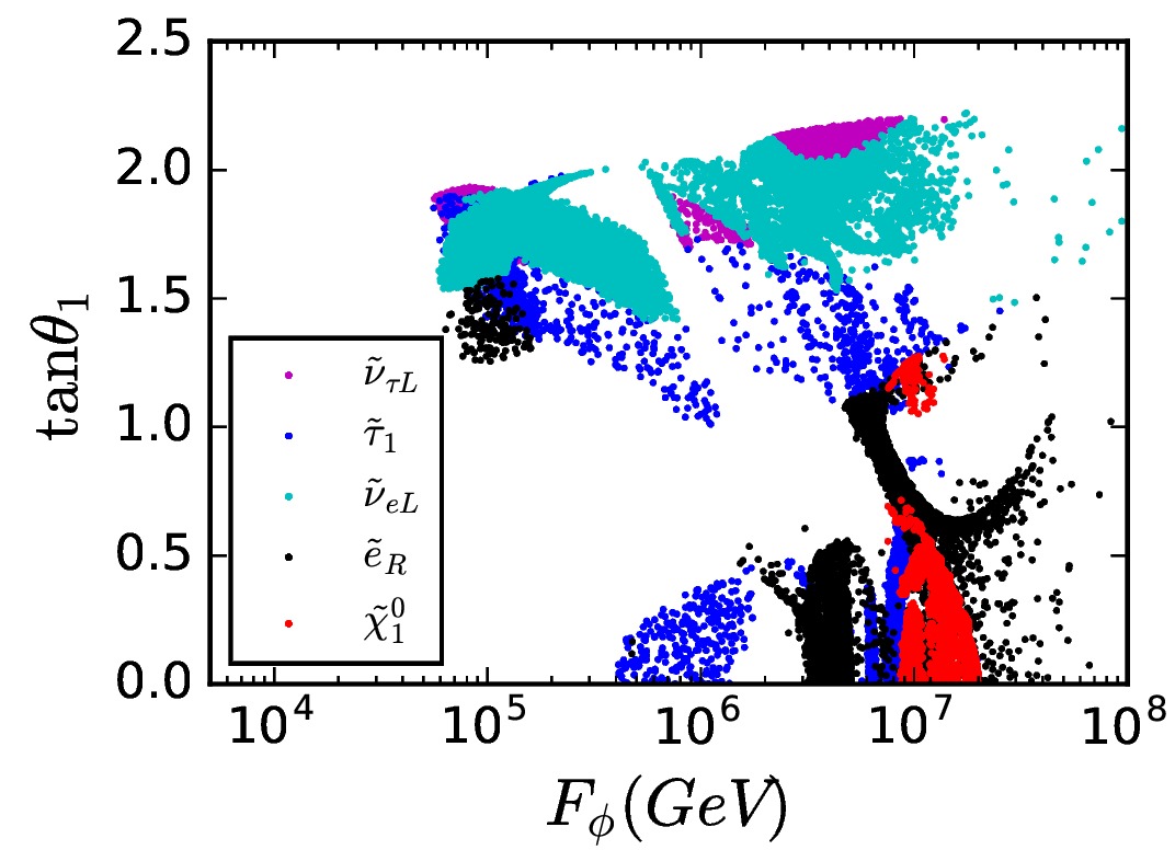
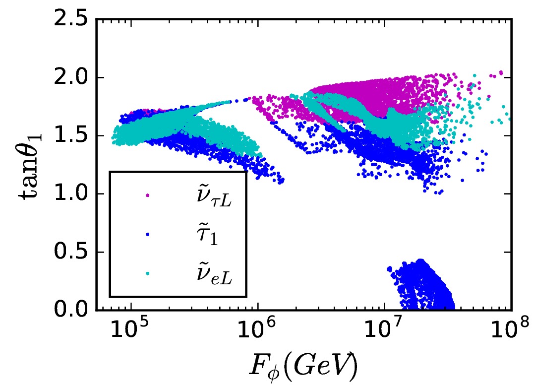
  Figure 1: Allowed regions of $\tan\theta_{1}$ vs $F_{\phi}$ with $a=3$ (left panel) and $a=2$ (right panel) in scenario I. All points satisfy the constraints from (I) to (III).

  

  

  

  

  

  

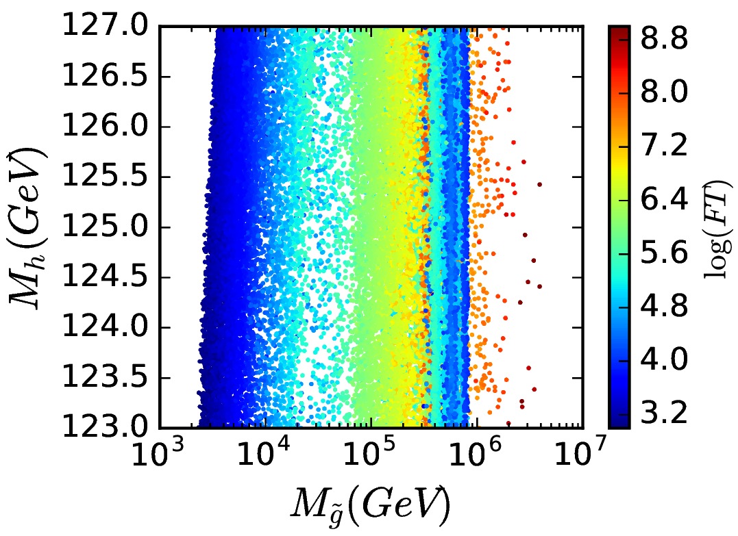
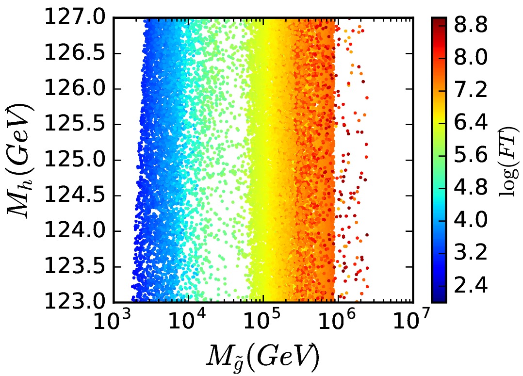
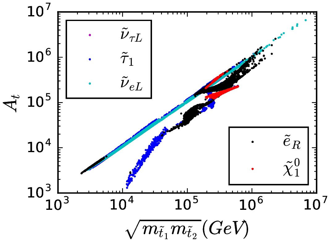
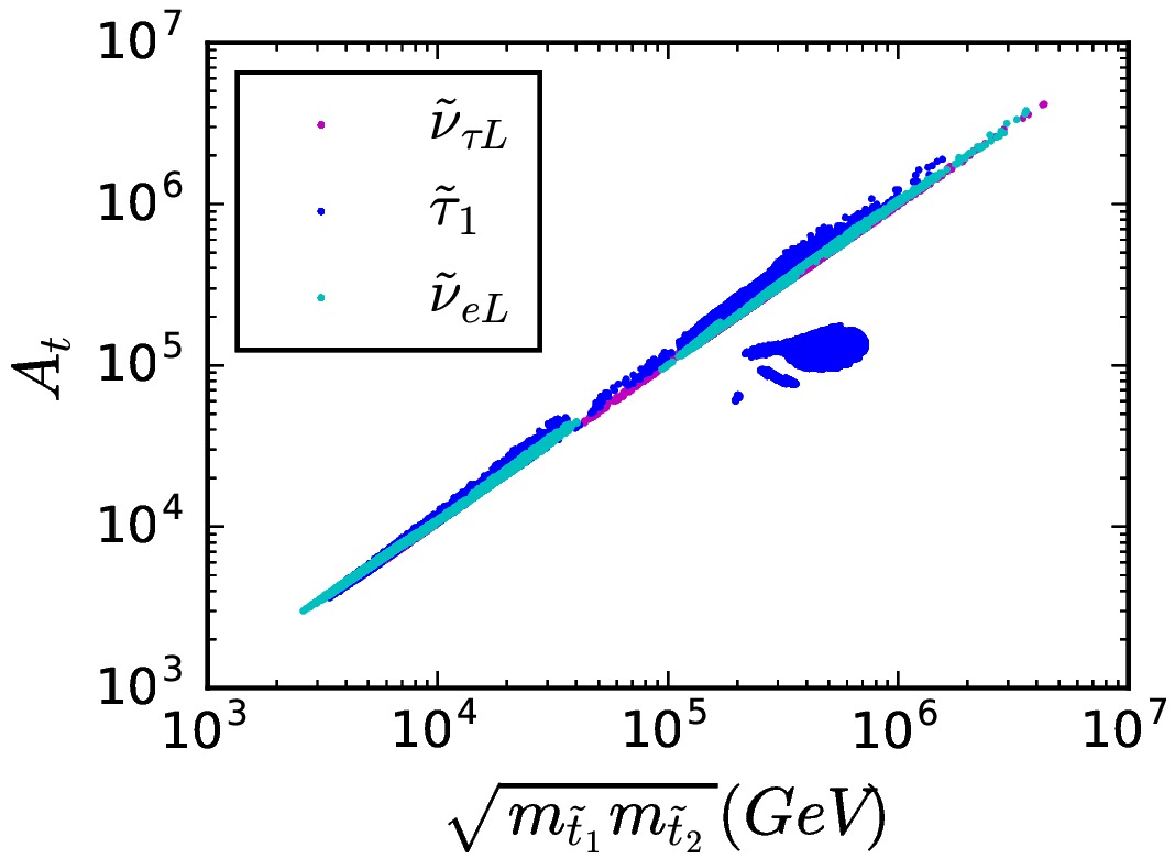
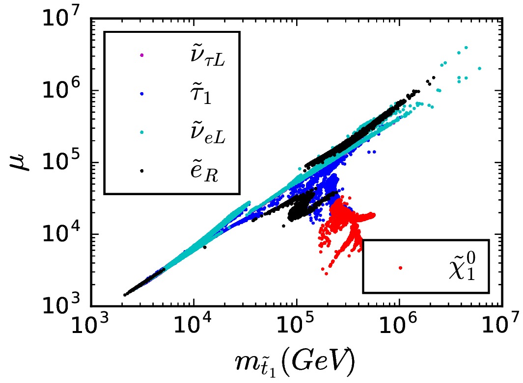
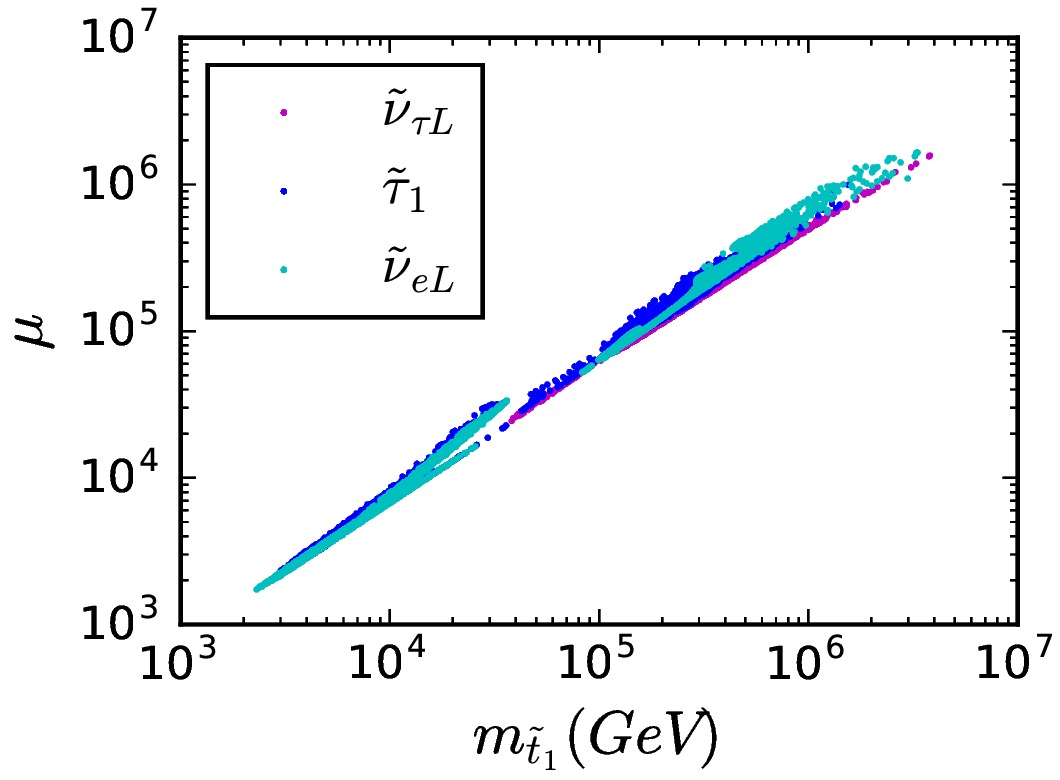
  Figure 2: Allowed regions for various LOSP with $a=3$ (left panel) and $a=2$ (right panel) in scenario I. All points satisfy the constraints from (I) to (III). In the upper panels, the BGFT measure is used to parameterize the level of EWFT.

• The Higgs mass in MSSM is given by

  $$m_{h}^{2}\simeq m_{Z}^{2}\cos^{2}2\beta+\frac{3m_{t}^{4}}{4\pi^{2}v^{2}}\left[\log\frac{M_{\mathrm{SUSY}}^{2}}{m_{t}^{2}}+\frac{\tilde{A}_{t}^{2}}{M_{\mathrm{SUSY}}^{2}}\left(1-\frac{\tilde{A}_{t}^{2}}{12M_{\mathrm{SUSY}}^{2}}\right)\right],$$ (103)

  with $\tilde{A}_{t}\equiv A_{t}-\mu\cot\beta$ and $M_{\mathrm{SUSY}}=\sqrt{m_{\tilde{t}_{1}}m_{\tilde{t}_{2}}}$ the geometric mean of stop masses. To increase the loop contributions to the Higgs mass, we can either choose $M_{\mathrm{SUSY}}/m_{t}\gg 1$ or $M_{\mathrm{SUSY}}/m_{t}>1$ with $\tilde{A}_{t}/M_{\mathrm{SUSY}}>1$. Without stop mixing, the stop masses have to be heavier than $5$ TeV.

  The Higgs mass $m_{h}$ versus the gluino mass $m_{\tilde{g}}$ for the survived points are shown in the upper panels of figure 2. We also show the parameters $A_{t}$ vs $\sqrt{m_{\tilde{t}_{1}}m_{\tilde{t}_{2}}}$ in the middle panels of figure 2, which can be used to estimate the dominant loop contributions to the Higgs mass. We can see from the figures that it is fairly easy to accommodate the 125 GeV Higgs mass in our scenarios. As a large trilinear coupling $A_{t}$ at the messenger scale can be generated by eqn.(51) and eqn.(61), our scenario can accommodate the 125 GeV Higgs mass with the geometric mean of stop masses as low as 2 TeV. This is in contrast to ordinary GMSB scenario, which predicts a vanishing $A_{t}$ at the messenger scale and is difficult to accommodate the 125 GeV Higgs mass with such light stop masses (unless the messenger scale in GMSB is extremely high).

  Low value of $F_{\phi}$, which sets the whole soft SUSY spectrum including the stop masses to be light, needs low electroweak fine-tuning(EWFT). The involved Barbier-Giudice(BG) FT measuresBGFT are shown with different colors. In our sceanrio, the least BGFT value can be ${\cal O}(10^{3})$. To see more clearly the EWFT, we plot the parameter $\mu$ vs $m_{\tilde{t}_{1}}$ in the bottom panels of figure 2. Low EWFT in general corresponds to low value of $\mu$.

• As noted previously, the LOSP in our scenarios can be the $\tilde{\nu}_{eL},\tilde{e}_{R},\tilde{\tau}_{1}$ other than the lightest neutralino $\tilde{\chi}_{1}^{0}$. If the lightest neutralino is lighter than the axino, the $\chi_{1}^{0}$ LSP can act as the DM candidate. On the other hand, if axino is the LSP and act as the DM particle, the LOSP can later decay into axino after its freezing out. The relic density of axino is therefore related to that of LOSP by

  $$\Omega_{\tilde{a}}h^{2}=\frac{m_{\tilde{a}}}{m_{LOSP}}\Omega_{LOSP}h^{2}~{}.$$ (104)

  

  

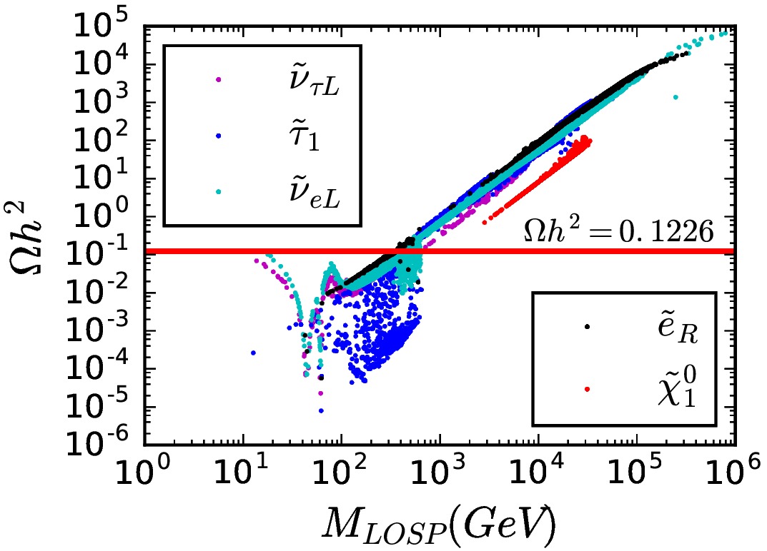
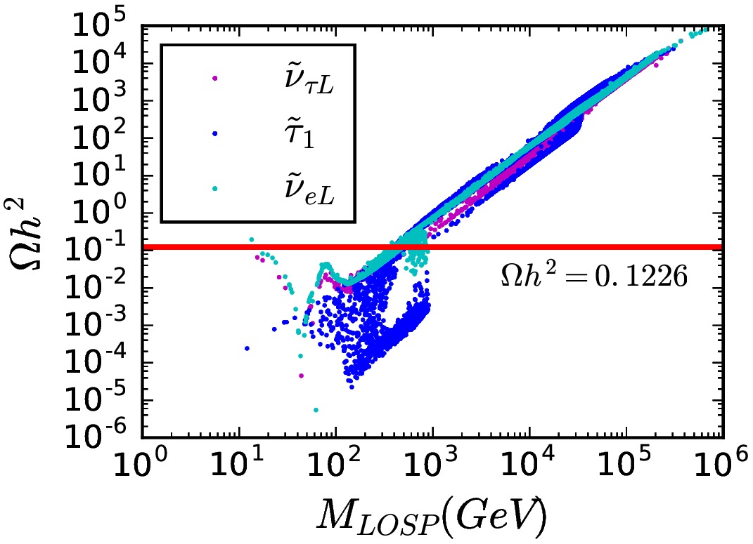
  Figure 3: The relic abundances of various LOSP particles for $a=3$ (left panel) and $a=2$ (right panel) in scenario I.

  The relic abundances of those various LOSP are shown in figure 3. We can see from the figure that the lightest neutralino can serve as the LOSP for $a=3$. However, $\chi_{1}^{0}$ particle, if it is also the LSP, has a relic abundance exceeding the DM upper bound and is therefore ruled out as the DM particle. Axino DM scenario, on the other hand, is still allowed. It can be seen from equation (104) that the LSP relic abundance is always smaller than that of the LOSP. So, if axino is the LSP, the $\chi_{1}^{0}$ LOSP can decay into the axino and its relic density can therefore possibly lead to a right amount of axino DM. Other LOSP species, such as $\tilde{e}_{R},\tilde{\tau}_{1}$, can not be the DM candidates because they are not electric neutral. The left-handed sneutrino DM scenario had already be rule out by DM direct detection experiments. All of these LOSPs can decay into axino DM particle after they freeze out if the axino is the true LSP.

  It is hopeless to detect the axino DM via DM direct detection experiments and collider experiments because of its extremely weak interaction strength. However, the axino DM may show up its existence from the properties of the LOSP. The LOSP typically decays into axino with a lifetime less than one second and practically be stable inside the collider detector. The electrically charged particle would appear as a stable particle inside the detector. The injection of high-energetic hadronic and electromagnetic particles, produced from late decays of the LOSP into axino (with lifetime less than one second), will not affect the abundance of light elements produced in the Big Bang Nucleosynthesis(BBN) era.

Scenario II:

Similar discussions can be carry out for Scenario II. Allowed regions of $\tan\theta_{2}$ versus $F_{\phi}$ for various types of the LOSP are marked with various colors in figure 4. As scenario I, the survived regions admit $\tilde{\nu}_{eL},\tilde{e}_{R},\tilde{\tau}_{1},\chi_{1}^{0}$ as the LOSP. Besides, the 125 GeV Higgs can also be accommodated easily in this scenario. In fact, as can be seen in the middle panels of figure 5, $\sqrt{m_{\tilde{t}_{1}}m_{\tilde{t}_{2}}}$ can be as low as 3 TeV with an intermediate large value of $A_{t}$. From the allowed ranges of the $\mu$ vs $m_{\tilde{t}_{1}}$ parameters, it is clear that the case $a=3$ can adopt relatively light $\mu$ in compare with the case $a=2$, therefore less EWFT. This observation is consistent with the conclusion from the values of the BGFT measure in the upper panels of figure 5.

The freeze out relic density for various LOSP are shown in figure 6. Again, the lightest neutralino $\tilde{\chi}_{1}^{0}$ (in $a=3$ case) LOSP can not be the DM candidate because its relic abundance will over close the universe. If the axino is the LSP and act as the DM particle, the LOSP can later decay into axino after its freezing out.

Figure 4: Allowed regions of $\tan\theta_{2}$ vs $F_{\phi}$ with $a=3$(left panel) and $a=2$(right panel) in scenario II. All points satisfy the constraints from (I) to (III).

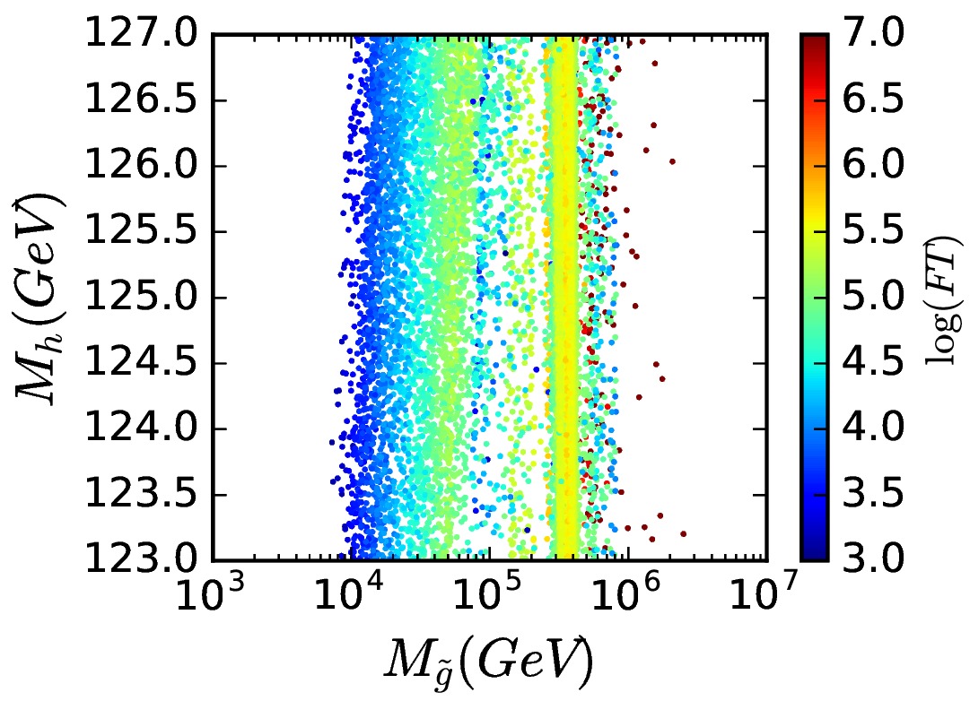
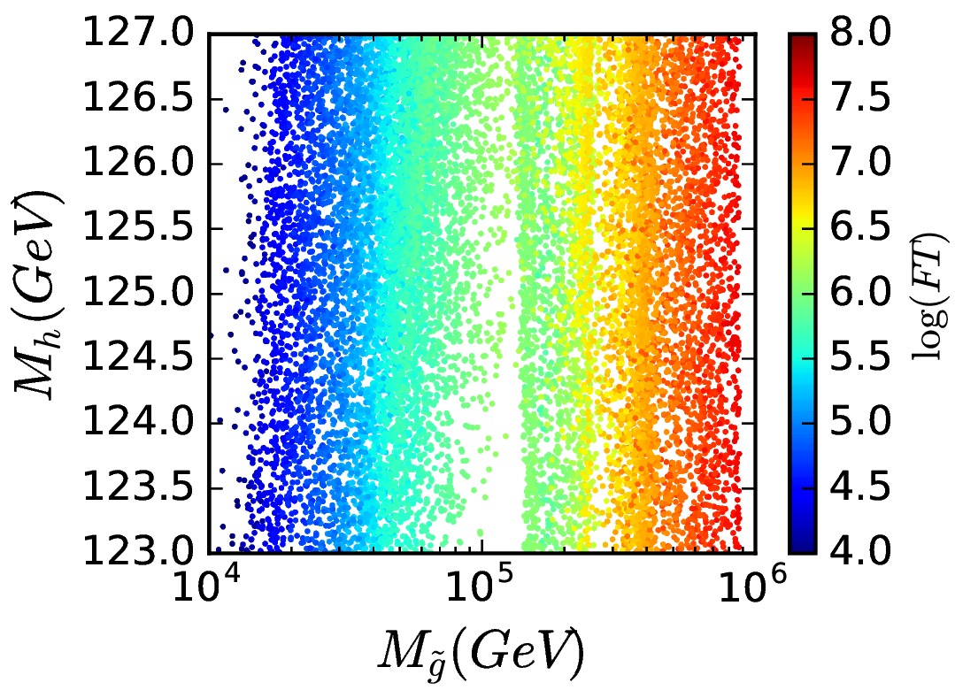
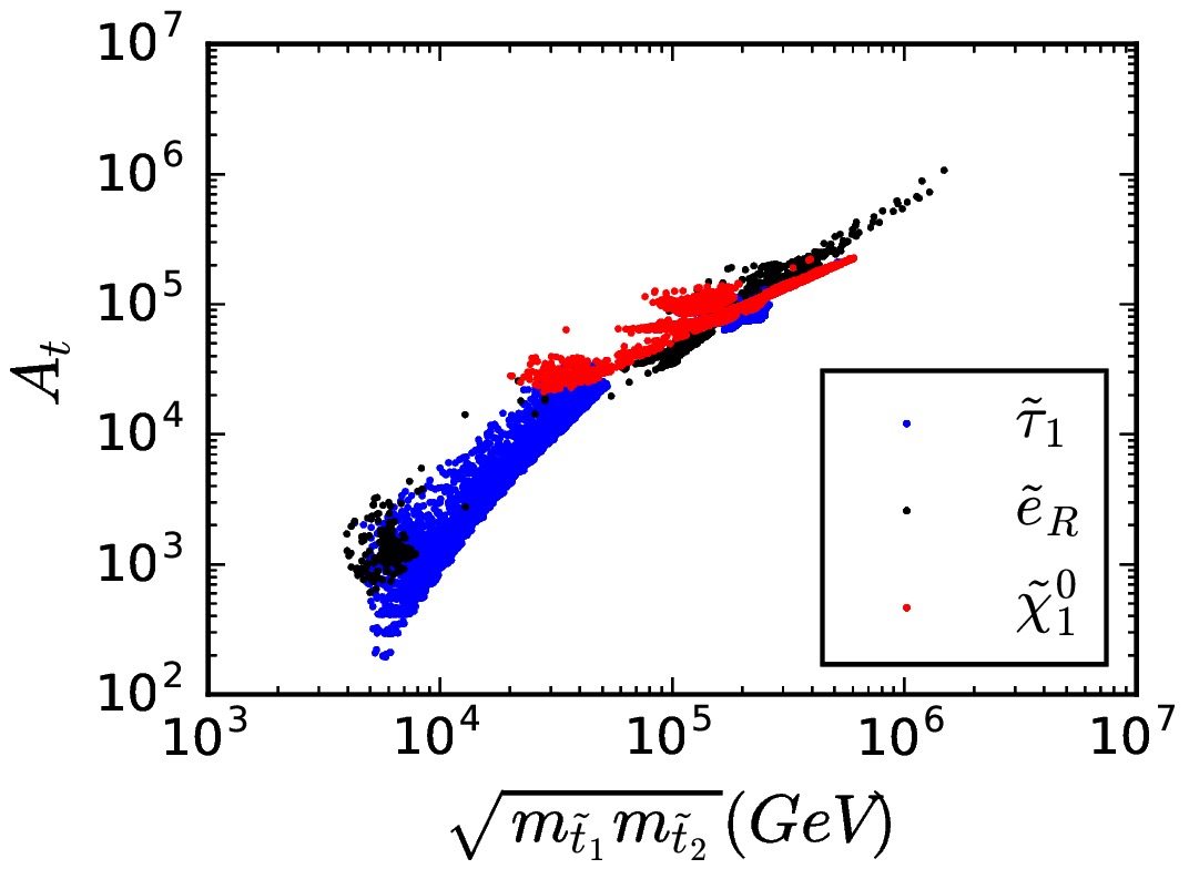
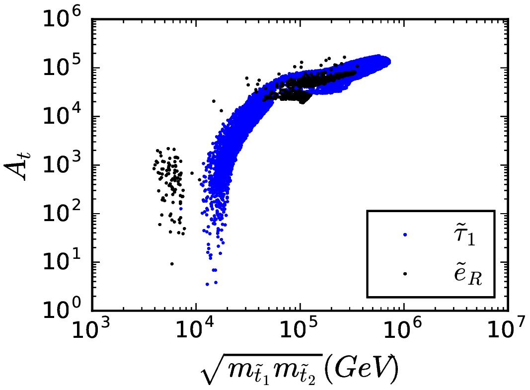
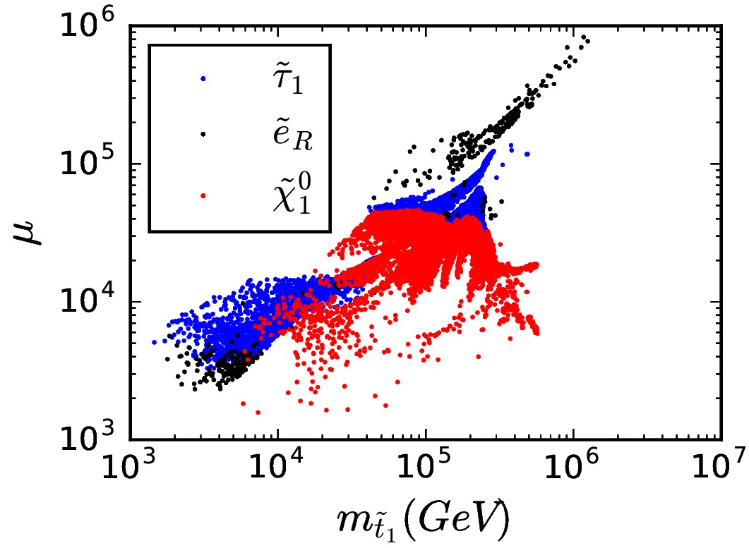
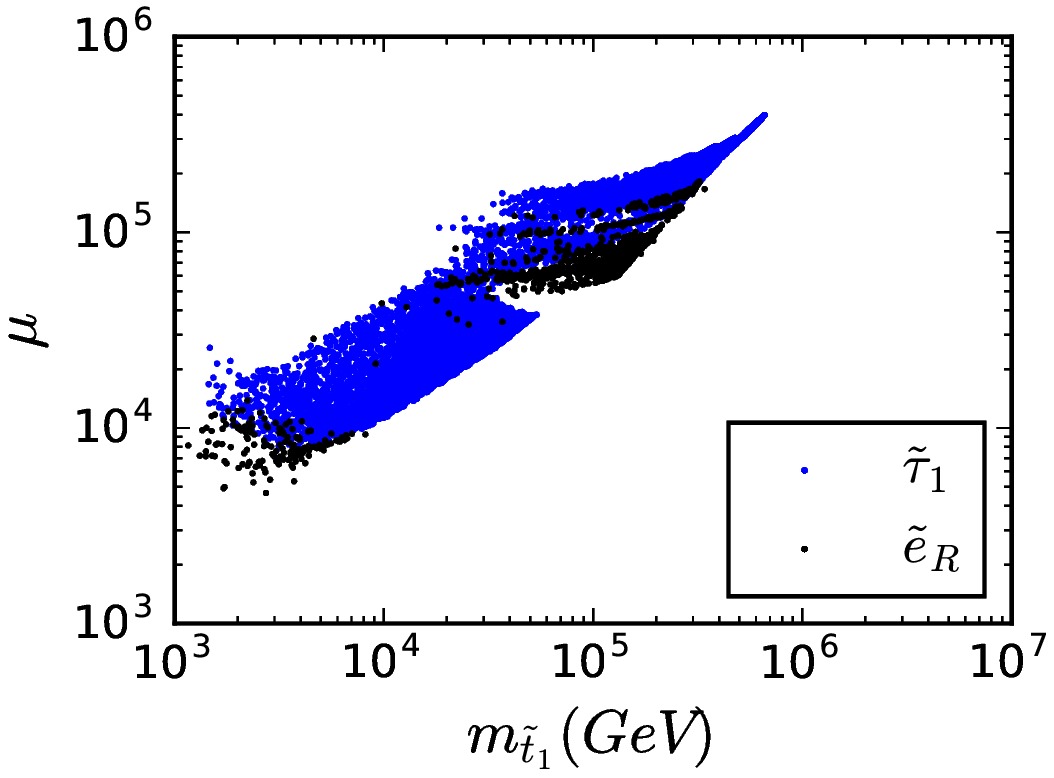
Figure 5: Allowed regions for various LOSP with $a=3$ (left panel) and $a=2$ (right panel) in scenario II. All points satisfy the constraints from (I) to (III). In the upper panels, the BGFT measure is used to parameterize the level of EWFT.

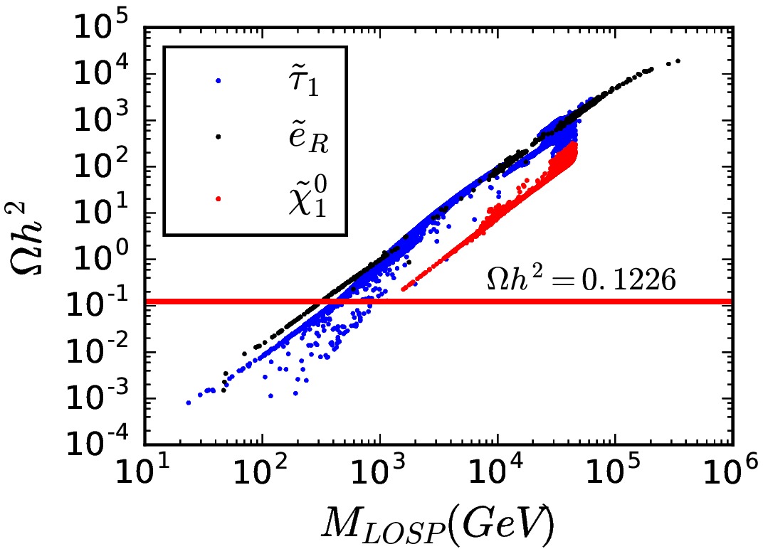
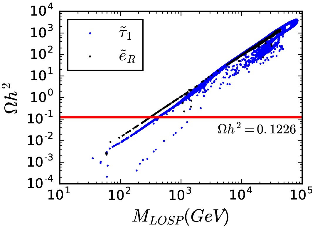
Figure 6: The relic abundances of various LOSP particles for $a=3$(left panel) and $a=2$(right panel) in scenario II.

5 Conclusions

We propose a minimal Yukawa deflection scenario of AMSB from the Kahler potential through the Higgs-messenger mixing. Salient features of this scenario are discussed and realistic MSSM spectrum can be obtained. Such a scenario, which are very predictive, can solve the tachyonic slepton problem with less messenger species. Numerical results indicate that the LOSPs predicted by this scenario can not be good DM candidates. So it is desirable to extend this scenario with a Peccei-Quinn sector to solve the strong CP problem and at the same time provide new DM candidates. We propose a way to obtain a light axino mass in SUSY KSVZ axion model with (deflected) anomaly mediation SUSY breaking mechanism. The axino can possibly be the LSP and act as a good DM candidate.