Effective reinforcement learning based local search for the maximum $k$-plex problem

Abstract

The maximum $k$-plex problem is a computationally complex problem, which emerged from graph-theoretic social network studies. This paper presents an effective hybrid local search for solving the maximum $k$-plex problem that combines the recently proposed breakout local search algorithm with a reinforcement learning strategy. The proposed approach includes distinguishing features such as: a unified neighborhood search based on the swapping operator, a distance-and-quality reward for actions and a new parameter control mechanism based on reinforcement learning. Extensive experiments for the maximum $k$-plex problem ($k=2,3,4,5$) on 80 benchmark instances from the second DIMACS Challenge demonstrate that the proposed approach can match the best-known results from the literature in all but four problem instances. In addition, the proposed algorithm is able to find 32 new best solutions.

Keywords: Heuristic, Local search, Reinforcement Learning, NP-hard, $k$-plex

1 Introduction

Let $G=(V,E)$ be a simple undirected graph, where $V=\{v_{1},\ldots,v_{n}\}$ is the set of vertices and $E\subset V\times V$ is the set of edges. A $k$-plex for a given positive integer $k$ is a subset $S$ of $V$ such that each vertex of $S$ is adjacent to at least $|S|-k$ vertices in the subgraph $G[S]=(S,E\cap S\times S)$ induced by $S$. Formally, let $N(v)$ be the set of adjacent vertices $v_{i}$ of $v$ (i.e., $\{v_{i},v\}\in E$), the maximum $k$-plex problem with any fixed $k\geq 1$ ($k\in Z^{+}$) aims to find a $k$-plex $S$ of maximum cardinality, such that $\forall v\in S,|N(v)\cap S|\geq|S|-k$. The $k$-plex problem first aroses in the context of graph theoretic social network [22] and has become popular in several other contexts [6, 7, 9]. The $k$-plex problem with any fixed positive integer $k$ is an NP-complete problem [2], it reduces to the well-known maximum clique problem (MC) when $k=1$, one of Karp’s 21 NP-complete problems [15]. The $k$-plex problem has a number of applications in information retrieval, code theory, signal transmission, social networks, classification theory amongst others [8, 16, 20, 26].

Due in part to the wide variety of real-world applications, increased research effort is being devoted to solving this problem. Over the past few years, several exact algorithms have been proposed for finding the maximum $k$-plex of a given graph [2, 17, 19, 24, 26]. These methods can find optimal solutions for graphs with around a thousand vertices in a reasonable amount of computing time (within 3 hours). However, they often fail to solve larger instances of the problem. On the other hand, several heuristic approaches have also been presented, which are able to find high-quality solutions for larger problem instances [10, 18, 28]. Two of these approaches [10, 18] are based on the general GRASP framework [21], whilst the other [28] uses the tabu search metaheuristic.

One notices that, compared to the research effort on the MC problem, studies for the maximum $k$-plex problem are more recent and less abundant. In this work, we are interested in approximately solving the representative large scale $k$-plex instances by presenting an effective heuristic approach. Moreover, the reinforcement learning techniques are shown to be able to improve the performance of local search algorithms [5, 27], hereby, we are also interested in investigating the reinforcement learning based local search for solving the maximum $k$-plex problem. We apply the recent breakout local search and the reinforcement learning together to explore the search space (denoted as BLS-RLE). It uses descent search to discover local optima before applying sophisticated diversification strategies to move to unexplored regions of the search space. BLS-RLE integrates several distinguishing features to ensure that the search process is effective. Firstly, a reinforcement learning technique is applied to adaptively and interdependently control three parameters deciding the type of perturbation to be applied and the magnitude of that perturbation. Secondly, the search is driven by a unified ($q$,1)-swap($q$ $\in$ $Z$) operator, used to explore the constrained neighborhoods of the problem. Finally, a distance-and-quality reward is used to maintain a high-quality set of parameters based on previous experience.

We evaluate BLS-RLE for the $k$-plex problem (with $k=2,3,4,5$) on a set of 80 large and dense graphs from the second DIMACS Challenge benchmark. Comparisons are performed to a number of state-of-the art methods from the literature, and the computational results show that BLS-RLE is able to achieve the best-known results for all the instances tested except 4 cases. In particular, BLS-RLE finds 11 new best solutions for $k=2$, 7 for $k=3$, 7 for $k=4$ and 7 for $k=5$ respectively.

The rest of the paper is organized as follows. Section 2 presents the proposed reinforcement learning based local search algorithm for solving the maximum $k$-plex problem. Section 3 shows the computational results of BLS-RLE for the $k$-plex problem with $k=2,3,4,5$ and comparisons with the state-of-the-art algorithms in the literature. Before concluding, Section 5 investigates and analyzes the influence of reinforcement learning for the local search algorithm.

2 The reinforcement learning based local search algorithm

The proposed reinforcement learning based local search algorithm (BLS-RLE) follows the recent general learning based local search framework, which was first introduced by [5] and applied to the Vertex Separator Problem. BLS-RLE combines an intensification stage that applies descent local search, with a distinctive diversification stage that adaptively selects between two or more perturbation operators with a particular perturbation magnitude. The type of perturbation operator (denoted as $e$), the number of perturbation moves (the depth of perturbation, denoted as $l$) and the degree of random perturabtion (denoted as $b$) are three important self-adaptive parameters that control the degree of diversification during perturbation. The combination of these three parameters by determining the values of $l$, $e$ and $b$ independently may not constitute the most suitable degree of diversification required at one stage of the search. And [12] highlights the automated configuration and parameter tuning techniques are very important for effectively solving difficult computational problems. Hence, unlike the parameter tuning techniques introduced in [12], BLS-RLE uses a parameter control mechanism based on reinforcement learning [1] to adaptively and interdependently determine the value of parameters.

2.1 General procedure

The overall BLS-RLE algorithm is summarized in Algorithm 1. Following the Prelearning phase, the first step of each iteration of BLS-RLE consists of selecting an action (parameter triple $(l,e,b)$) according to the Softmax action-selection rule [23] (line 4). Although we use Softmax, any action selection model could be used as an alternative. The diversification procedure is then applied to the current local optimum $S$ using $(l,e,b)$ (line 5), followed by the $Intensification$ (descent local search) to improve the quality of the perturbed solution $S^{\prime}$ (line 6). Furthermore, a global variable $S^{*}$ is used to record the best $k$-plex solution discovered during the search (lines 7-9). Finally, BLS-RLE applies the $DetermineParameterTripleReward$ procedure to determine the reward $r$ for the selected action (parameter triple) with regard to $S$ by considering both the quality and the diversity criterion (line 10). Finally, the action value corresponding to $(l,e,b)$ is updated with $r$ (line 11).

Algorithm 1 General procedure of BLS-RLE for the maximum $k$-plex problem

0:  A graph $G=(V,E)$, an integer $k$

0:  The largest $k$-plex $S^{*}$ found

1:  $(P_{learn},S)$ $\leftarrow$ $Prelearning$(); /* $P_{learn}$ is a set of parameter triples $\{(l_{0},e_{0},b_{0}),(l_{1},e_{1},b_{1}),\ldots\}$, $S$ is a feasible $k$-plex */

2:  $Max\leftarrow|S|;$

3:  $Iter\leftarrow 0$;

4:  repeat

5:     $(l,e,b)\leftarrow SelectParameterTriple()$;

6:     $S^{\prime}\leftarrow Diversification(l,e,b,S)$;

7:     $S\leftarrow Intensification(S^{\prime})$;

8:     if $|S|>|S^{*}|$ then

9:        $S^{*}\leftarrow S;Max\leftarrow|S^{*}|;$

10:     end if

11:     $r\leftarrow DetermineParameterTripleReward(S)$;

12:     $ApplyReward(r)$;

13:     if $Iter>\epsilon$ then

14:        $UpdateParameterTriple()$;

15:        $Iter\leftarrow 0$;

16:     end if

17:     $Iter\leftarrow Iter+1$;

18:  until a stop criterion is met

19:  return  the best found $S^{*}$;

A parameter triple $(l,e,b)$ determines the perturbation type, perturbation magnitude and degree for diversification, where $l$ represents the number of perturbation moves, $e$ represents the probability of selecting one type of perturbation operator over another and $b$ represents the degree of random perturbation to adjust the strength of random peturbation. The set $P_{all}$ contains all possible parameter triples, i.e., $P_{all}=\{(l_{0},e_{0},b_{0}),\ldots,(l_{m},e_{m},b_{m})\}$ where $m$ is the total number of triples to be generated. Here we use one of two types of perturbation operator, directed or random. A novel method for generating parameter triples is proposed, with the number of perturbation moves $lin\{l_{i}\}$ takes the following piecewise function (Eq. (1)). The linear nature of the first component reflects a more fine-grained approach to diversification, using a larger number of values when the perturbation level is low. As the perturbation level increases, the number of potential values for $l$ will decrease, with the values that they take increasing exponentially. This provides a greater level of diversification within a smaller number of potential $l$ values at the higher end.

$$\small l_{i}=\left\{\begin{array}[]{rcl}i+2&&{0\leq i<30}\\ 2^{i-25}&&{30\leq i<33}\end{array}\right.$$ (1)

This method for defining the set of potential $l$ values and subsequently triples in $P_{all}$ is in contrast to previous work [5], where a linear relationship between consecutive $l$ values is maintained throughout the range. As for the parameters $e$ and $b$, the value of $e$ ranges from 95 to 100, and $b$ ranges 70 to 90 respectively.

The algorithm uses a one-time $Prelearning$ procedure to evaluate the degree of diversification introduced by each parameter triple $(l,e,b)\in P_{all}$ that can be applied throughout the search process. For this purpose, the degree of diversification refers to the ability of the search to discover new local optima. To limit the number of possible actions and to reduce the time required to learn, BLS-RLE maintains a small subset $P_{learn}\subset P_{all}$ of $\kappa$ parameter triple, representing potential actions that can be performed at that time. $P_{learn}$ is periodically updated (every $\epsilon$ iterations) with a new parameter triple from $P_{all}\setminus P_{learn}$ based on the action values learned during the Prelearning procedure.

2.2 Prelearning procedure

Iterated Local Search is used to assess the diversification capability of each parameter triple $(l,e,b)$, based on how frequently a new local optimum is found. The number of times a previously encountered local optima is visited by each triple is recorded, with the value for each triple initially set to 0. The detailed procedure is as follows:

1. A perturbation operator is selected and applied, based on the parameter $e$. The perturbation operator makes $l$ moves, with a hash table used to record recently visited local optima as historical information.

2. Following this, descent local search attempts to improve the solution, returning the local optimum.

3. Finally, a check is performed to see if the local optimum has already been encountered. If so, the count of revisited local optima for the corresponding triple is increased by 1.

4. Repeat steps 1 to 3 until each parameter triple $(l,e,b)$ has been used.

This process is repeated $\alpha$ times, where $\alpha$ is chosen to provide enough samples from which a ranking of triples can be derived. Once completed, the parameter triples in $P_{all}$ are sorted in ascending order of the number of times they revisited previously encountered local optima, with the $n$ best-ranked triples kept in a set $P_{learn}$. Note that here $n$ is experimentally set to 2375, and that this ranking will also be used for the reward and value function.

2.3 Intensification of search

The intensification stage of BLS-RLE aims to find better solutions by descent local search. For this purpose, BLS-RLE employs the (0,1)-swap move operator to try to improve a solution. Recall that $N(v)$ is the set of adjacent vertices of $v$, let $V\backslash S$ be the complementary set of $S$ and $N(S)$ be the set of vertices in $V\backslash S$ that are adjacent to at least one vertex in $S$, i.e., $N(S)=\cup_{v\in S}N(v)\backslash S$. For a vertex $v$ in $S$, if $|N(v)\cap S|=|S|-k$, then $v$ is called a critical vertex. The set $NS_{0}$, shown in Eq. (2), consists of all vertices in $N(S)$ that are connected to at least $|S|-k+1$ vertices in $S$ and are also connected to all of the critical vertices $C$ [24, 28]. Descent local search includes a new vertex from $NS_{0}$ to increase the cardinality of the current $S$, while maintaining the feasibility of the $k$-plex. When $NS_{0}$ is empty, the intensification stage is complete and the local optimum found is returned.

$$\small NS_{0}=\{v\in N(S):|N(v)\cap S|\geq|S|-k+1,C\backslash N(v)=\emptyset\}$$ (2)

2.4 Perturbation operators

In order to escape from local optima, directed or random perturbations are used to guide the search towards unexplored regions. Directed perturbation aims to minimize the degradation of the $k$-plex cardinality, while random perturbation aims to move the search away from the current location. The choice of operator is based on the probability $e$ of using a directed perturbation operator, with random perturbation applied otherwise (with the corresponding probability 1 - $e$). If the random perturbation is chosen, the value of parameter $b$ controls the strength of random perturbation (the random perturbation is compared to a random start when $b\approx 0$). The number of perturbation moves is defined as $l$, with $l$, $e$ and $b$ controlled interdependently by the reinforcement learning strategy.

The proposed approach uses a unified $(q,1)-swap$ ($q=0,1,2,\ldots$) move to explore the search space. Four sets $NS_{i}$ $(i=0,1,2,3)$ are involved in this procedure as given below, $NS_{0}$ is already presented above. The $NS_{1}$ set consists of vertices $v$ that are adjacent to at least $|S|-k$ vertices in $S$, where $u$ is the unique critical vertex not adjacent to $v$, as shown in Eq. (3). $NS_{2}$ consists of vertices $v$ that are adjacent to exactly $|S|-k$ vertices in $S$. These $|S|-k$ vertices should include all of the critical vertices, as shown in Eq. (4) [28]. A corresponding exchanged vertex $u$ is randomly selected from $S\backslash N(v)$. The vertex from $N_{1}\cup N_{2}$ could be employed for the (1,1)-swap move operator, such that the search is guided to a new region while leaving the quality of solution unchanged. The $NS_{>2}$ consists of the vertex $v$, such that $v$ is in the set of $V\backslash S$ and $v$ is not included in the sets $NS_{0}$, $NS_{1}$ and $NS_{2}$. A corresponding exchanged vertex $u$ is selected from $S$ that will cause the $k$-plex to be infeasible after including $v$. The vertex from $NS_{3}$ could be used for the $(q,1)$-swap ($q\geq 2$) move in order to discover new and promising regions of the search space.

$$\small NS_{1}=\{v\in N(S):|N(v)\cap S|\geq|S|-k,|C\backslash N(v)|=1\}$$ (3)

$$\small NS_{2}=\{v\in N(S):|N(v)\cap S|=|S|-k,C\backslash N(v)=\emptyset\}$$ (4)

$$\small NS_{3}=\{v\in V\backslash({S\cup NS_{0}\cup NS_{1}\cup NS_{2}})\}$$ (5)

Directed perturbation applies a move from $NS_{0}\cup NS_{1}\cup NS_{2}\cup NS_{3}$, favoring moves that minimize the degradation of the cardinality of the current $k$-plex. Random perturbation applies a random move from $NS_{0}\cup NS_{3}$. Each move is only accepted when the quality is not worse than a given threshold, determined by the value of parameter $b$. A tabu list is used to prevent the search returning to previously visited locations. More precisely, each time a vertex is removed from the $k$-plex when employing the ($q$,1)-swap ($q\geq 2$), this vertex is prevented from moving back to $S$ for the next $tt_{1}$ iterations ($tt_{1}$ is called tabu tenure and $tt_{1}$ = 7). On the other hand, each time a vertex is removed from the $k$-plex when employing the (1,1)-swap, the tabu tenure is set to $tt_{2}=7+random(|NS_{1}\cup NS_{2}|)$ where $random(|NS_{1}\cup NS_{2}|)$ is a random integer from 1 to $|NS_{1}\cup NS_{2}|$.

2.5 Reward and value functions

After a locally optimal solution $S$ is returned by descent local search, we apply a distance-and-quality reward for each parameter triple (action). This reward considers both the quality of solution and the degree to which new areas of the search space are explored. The distance-and-quality reward $r_{i}$ is given in Eq. (6) [3]. The core motivation behind this strategy is to give the highest reward when new local optima are discovered with the minimum amount of diversification introduced. Recall that the parameter triples in $P_{all}$ are sorted in increasing order in the $Prelearning$ phase, the distance is determined by $\kappa-i$ where $i$ is the index $i$ of the parameter triple $(l,e,b)_{i}$ when $S$ is not stored in the hash table. The quality is evaluated by $(1-\frac{|S|-|S^{*}|}{|S^{*}|})^{2}\times 10$ where $|S|$ is the cardinality of the current $k$-plex $S$ and $S^{*}$ is the best solution found so far during the search.

$$\small r_{i}=\left\{\begin{array}[]{c}0,\qquad\qquad\qquad\qquad\textrm{If $S$ is already in the hash table}\\ \delta_{1}\times(\kappa-i)+\delta_{2}\times(1-\frac{|S|-|S^{*}|}{|S^{*}|})^{2}\times 10,\textrm{Otherwise}\\ \end{array}\right.$$ (6)

As soon as the reward $r_{i}$ for the parameter triple $(l,e,b)_{i}$ is computed, the $ApplyReward$ procedure is used to update the credit attributed to the action $(l,e,b)_{i}$ and accordingly compute the action value $\omega_{i}$. The values of $\omega_{i}$ are initialized to 1, and the 100 latest rewards ascribed to $(l,e,b)_{i}$ are used to estimate the credit that quantifies the performance of a particular action in a given period. According to this performance summary, the action value is updated.

2.6 Update of the parameter triple learning list

In order to prevent the search process from premature convergence, the parameter triple learning list should be updated periodically. Afterwards, the Softmax action-selection model [23] is used to select an action for the next iteration of the search.

The Softmax-based approach applies the Gibbs or Boltzmann distributions to assign a probability to each action in $P_{learn}$ [3]. The updating rule for the triple learning list first selects the worst parameter triple $a_{w}\in P_{learn}$, which has the lowest probability of selection. Then, the updating rule determines one promising parameter triple in $P_{all}\backslash P_{learn}$. According to the probabilities of actions in $P_{learn}$, we estimate the probability of each action in $P_{all}\backslash P_{learn}$ by a linear correspondence. For example, given 12 actions in $P_{all}$, 4 actions are selected from $P_{learn}$ and the probability of these 4 actions are known. We use a line to connect two adjacent actions whose probabilities are known, as shown in Figure 1. For action $a_{0}\in P_{all}\backslash P_{learn}$, the estimated probability of $a_{0}$ is obtained by the probability of the first action $a_{0}^{\prime}$ in $P_{learn}$ divided by the index of action $a_{0}^{\prime}$ in $P_{all}$. Similarly, the estimated probability of $a_{11}\in P_{all}\backslash P_{learn}$ is obtained by the probability of the last action $a_{3}^{\prime}$ in $P_{learn}$ divided by the difference between 11 and the index of action $a_{3}^{\prime}$ in $P_{all}$. Finally, we estimate the probability of all vertices in $P_{all}\backslash P_{learn}$ and select a vertex with a high probability to replace the worst action $a_{w}$ in $P_{learning}$. After the parameter triple learning list is updated, the actions in $P_{learn}$ are re-sorted, the action values are reset to 1, and the next round of search is triggered.

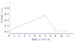
Figure 1: An illustrative example for estimating probability.

3 Experimental Set-up

In order to evaluate the performance of BLS-RLE, we conduct experiments on 80 benchmark instances from the Second DIMACS Implementation Challenge [13]. These instances were first established for the maximum clique (MC) problem and are frequently used for evaluating MC algorithms. As previously mentioned, the maximum $k$-plex problem can be reduced to the MC, hence these instances are also quite popular and challenging for evaluating solution methods to this problem.

The BLS-RLE algorithm is implemented in C++ and complied using g++ with the ‘-O3’ option under GNU/Linux running on an Intel Xeon E5440 processor (2.83GHz and 4GB RAM). When the DIMACS machine benchmarks are run on our machine, the run time required is 0.44, 2.63 and 9.85 seconds for graphs r300.5, r400.5 and r500.5 respectively. Each instance is run 20 times independently. The algorithm stops when a fixed cutoff time (180 seconds) is met. This experimental protocol is also used by a state-of-the-art heuristic in the literature [28]. BLS-RLE uses the self-adaptive parameters given in Table 1, all computational results were obtained with the same parameters. The adopted parameter settings are inspired by a previous method from the literature [5], where a parameter sensitivity analysis during the search guidance was provided.

Table 1: Parameter settings of BLS-RLE

Parameter	Description	Value
$\kappa$	the size of the learning parameter triple set $P_{learn}$	6
$\alpha$	the number of pre-learning iterations for each triple in $P_{all}$	100
$\tau$	the temperature of the Softmax-based adaptive procedure	2
$\epsilon$	the update frequency of the parameter triple learning list	4000
$\delta_{1}$	coefficient for reward function	2
$\delta_{2}$	coefficient for reward function	1

In addition to BLS-RLE we also provide the results of BLS-RND, a variant of BLS where the values of the two parameters, $l$, $e$ and $b$ are determined randomly. [14] highlighted the importance of comparing adaptive parameter control mechanisms with random sampling of the parameter space. When introducing a dynamic parameter control strategy, rather than using static parameter values, it is not clear whether it is the adaptive strategy or simply that the value of parameter is changing dynamically over time that is having an effect on performance.

4 Experimental Results

To assess the performance of BLS-RLE, we compare it with some state-of-the-art algorithms from the literature [2, 17, 19, 24, 28]. The experimental platform of [2] was performed on Dell Precision PWS690 machine with a 2.66GHz Xeon Processor, 3 GB RAM and 120 GB HDD. The experimental platform of [17, 19] was performed on a 2.2 GHz Dual-Core AMD Opteron Processor with 3GB memory, a AMD Athlon 64 3700+ machine with 2.2 GHz and 3GB memory respectively. The experimental platform of [24] was run on an Intel $Core^{TM}$2 Quad 3 GHz Processor with 4GB RAM, a 2.5 GHz Intel Core i5-3210M processor with 4GB memory respectively. The experimental platform of [28] was run on an AMD Opteron 4184 with 2.8 GHz Processor with 2GB RAM. Table 2, 9, 10 and 11 compare BLS-RLE to several recent best-performing algorithms and the heuristic method proposed in [28] (FD-TS) for $k=2,3,4,5$, covering the best known results for all of the instances tested.

Table 2: Comparisons of BLS-RLE for the $k$-plex when $k$=2

Instance	BEV	FD-TS			BLS-RLE
		Max (Avg.)	Time(s)		Max (Avg.)	Time(s)
brock200_1	25	26	0.15		26	0.04
brock200_2	13	13	0.01		13	0.01
brock200_3	17	17	0.02		17	0.02
brock200_4	20	20	0.06		20	0.03
brock400_1	23	30	0.42		30	0.16
brock400_2	27	30	0.51		30	0.11
brock400_3	-	30	0.35		30	0.20
brock400_4	27	33 (31.2)	64.18		31	23.83
brock800_1	-	25	10.90		25	2.26
brock800_2	-	25	11.36		25	1.82
brock800_3	-	25	12.68		25	2.28
brock800_4	-	26 (25.55)	56.21		26 (25.9)	51.07
C1000.9	-	81 (80.55)	39.65		82 (81.75)	51.66
C125.9	-	43	0.00		43	0.01
C2000.5	-	19 (18.95)	27.96		20 (19.05)	15.00
C2000.9	-	90 (88.9)	65.21		93 (91.7)	76.41
C250.9	-	55	8.43		55	12.96
C4000.5	-	20	39.23		21 (20.15)	11.86
C500.9	-	69	10.67		69	2.78
c-fat200-1	12	12	0.00		12 (10.75)	0.01
c-fat200-2	24	24	0.01		24 (22.25)	0.02
c-fat200-5	58	58	0.01		58 (57.4)	0.01
c-fat500-10	126	126	0.08		126 (124.95)	0.02
c-fat500-1	14	14	0.00		14 (12.4)	0.01
c-fat500-2	26	26	0.00		26 (25.2)	0.01
c-fat500-5	64	64	0.02		64 (62.45)	0.01
DSJC1000_5	-	18	26.61		18	13.37
DSJC500_5	-	16	0.29		16	0.18
gen200_p0.9_44	-	53	0.14		53	0.38
gen200_p0.9_55	-	57	0.02		57	0.04
gen400_p0.9_55	-	68 (67.7)	65.76		68	40.14
gen400_p0.9_65	-	73 (71.6)	28.01		74 (72.75)	44.32
gen400_p0.9_75	-	79 (78.05)	30.62		80 (79.1)	35.22
hamming10-2	512	512	8.97		512	1.96
hamming10-4	41	48	1.53		48	0.45
hamming6-2	32	32	0.00		32	0.01
hamming6-4	6	6	0.00		6	0.01
hamming8-2	128	128	0.09		128	0.02
hamming8-4	16	16	0.01		16	0.01
johnson16-2-4	10	10	0.00		10	0.00
johnson32-2-4	-	21	0.02		21	0.00
johnson8-2-4	5	5	0.00		5	0.00
johnson8-4-4	14	14	0.00		14	0.02
keller4	15	15	0.00		15	0.01
keller5	-	31	0.09		31	0.10
keller6	-	63	3.60		63	3.19
MANN_a27	236	236 (235.9)	12.64		236	0.13
MANN_a45	662	662 (661.4)	5.46		662	6.61
MANN_a81	-	2162 (2113.9)	139.35		2162	12.33
MANN_a9	26	26	0.00		26	0.01
p_hat1000-1	-	13	0.28		13	0.08
p_hat1000-2	-	56	0.43		56	0.32
p_hat1000-3	-	82	0.33		82	0.17
p_hat1500-1	-	14	1.46		14	0.33
p_hat1500-2	-	80	1.75		80	0.95
p_hat1500-3	-	114	0.61		114	0.16
p_hat300-1	10	10	0.00		10	0.02
p_hat300-2	30	30	0.01		30	0.03
p_hat300-3	43	44	0.07		44	0.05
p_hat500-1	12	12	0.06		12	0.03
p_hat500-2	-	42	0.02		42	0.02
p_hat500-3	-	62	0.18		62	0.06
p_hat700-1	13	13	0.06		13	0.07
p_hat700-2	50	52	0.06		52	0.03
p_hat700-3	73	76	0.54		76	0.14
san1000	-	17	9.39		18 (16.75)	50.68
san200_0.7_1	-	31	0.59		31	0.05
san200_0.7_2	24	26 (25.4)	9.74		26	0.10
san200_0.9_1	90	90	0.01		90	0.01
san200_0.9_2	-	71	2.47		71 (69.35)	2.03
san200_0.9_3	-	54 (53.95)	72.31		54	7.16
san400_0.5_1	-	15	1.24		15 (14.9)	9.08
san400_0.7_1	-	41	0.20		42 (41.55)	10.27
san400_0.7_2	-	32	7.22		33 (32.45)	36.36
san400_0.7_3	-	27 (26.3)	12.27		28 (27.75)	66.10
san400_0.9_1	-	102 (101.3)	9.09		103 (102.6)	39.24
sanr200_0.7	-	22	0.01		22	0.04
sanr200_0.9	-	51	0.61		51	0.17
sanr400_0.5	-	15	0.02		15	0.03
sanr400_0.7	-	26	1.03		26	0.34

Table 3: Comparisons of BLS-RLE for the $k$-plex when $k$=2

Benchmark set	BEV		FD-TS			BLS-RLE
	#max		#max	#avg.		#max	#avg.
brock (12 instances)	3		12	10		11	10
C (7 instances)	0		3	3		7	3
c-fat (7 instances)	7		7	7		7	0
DSJC (2 instances)	0		2	2		2	2
gen (5 instances)	0		3	2		5	3
hamming (6 instances)	5		6	6		6	6
johnson (4 instances)	3		4	4		4	4
keller (3 instances)	1		3	3		3	3
MANN (4 instances)	3		4	1		4	4
phat (15 instances)	4		15	15		15	15
san (11 instances)	1		6	4		11	4
sanr (4 instances)	0		4	4		4	4

Table 4: Comparisons of BLS-RLE for the $k$-plex when $k$=3

Benchmark set	BEV		FD-TS			BLS-RLE
	#Max		#Max	#Avg.		#Max	#Avg.
brock (12 instances)	1		11	9		12	9
C (7 instances)	0		3	2		7	3
c-fat (7 instances)	7		7	7		7	0
DSJC (2 instances)	0		2	2		2	2
gen (5 instances)	0		5	4		5	2
hamming (6 instances)	5		6	6		6	6
johnson (4 instances)	3		4	4		4	4
keller (3 instances)	1		2	2		3	3
MANN (4 instances)	3		4	3		4	4
phat (15 instances)	2		15	15		15	15
san (11 instances)	1		10	8		11	2
sanr (4 instances)	0		4	4		4	4

Table 5: Comparisons of BLS-RLE for the $k$-plex when $k$=4

Benchmark set	BEV		FD-TS			BLS-RLE
	#Max		#Max	#Avg.		#Max	#Avg.
brock (12 instances)	0		11	8		12	9
C (7 instances)	0		2	2		7	2
c-fat (7 instances)	7		7	7		7	0
DSJC (2 instances)	0		2	1		2	1
gen (5 instances)	0		5	5		5	2
hamming (6 instances)	3		6	5		5	4
johnson (4 instances)	3		4	4		4	4
keller (3 instances)	0		2	1		3	1
MANN (4 instances)	3		4	3		4	4
phat (15 instances)	1		15	14		15	15
san (11 instances)	1		11	9		11	2
sanr (4 instances)	0		4	4		4	4

Table 6: Comparisons of BLS-RLE for the $k$-plex when $k$=5

Benchmark set	BEV		FD-TS			BLS-RLE
	#Max		#Max	#Avg.		#Max	#Avg.
brock (12 instances)	0		12	8		12	11
C (7 instances)	0		3	2		7	3
c-fat (7 instances)	7		7	7		7	1
DSJC (2 instances)	0		2	1		2	1
gen (5 instances)	0		5	5		5	2
hamming (6 instances)	2		6	4		6	4
johnson (4 instances)	1		4	4		4	4
keller (3 instances)	0		3	2		3	1
MANN (4 instances)	2		3	3		4	4
phat (15 instances)	0		13	12		15	12
san (11 instances)	1		11	10		10	6
sanr (4 instances)	0		4	4		4	4

Table 7: New best results for DIMACS instances by BLS-RLE

	Instance	Maxpre	Max			Instance	Maxpre	Max
$k$ = 2	C1000.9	81	82		$k$ = 4	brock800_4	33	34
	C2000.5	19	20			C1000.9	107	109
	C2000.9	90	93			C2000.5	25	26
	C4000.5	20	21			C2000.9	118	123
	gen400_p0.9_65	73	74			C4000.5	26	27
	gen400_p0.9_75	79	80			C500.9	92	93
	san1000	17	18			keller6	107	112
	san400_0.7_1	41	42		$k$ = 5	C1000.9	119	122
	san400_0.7_2	32	33			C2000.9	132	137
	san400_0.7_3	27	28			C4000.5	29	30
	san400_0.9_1	102	103			C500.9	103	104
$k$ = 3	brock800_1		30			MANN_a81	3135	3240
	C1000.9	95	96			p_hat1500-3	164	165
	C2000.5	22	23			p_hat500-3	89	90
	C2000.9	105	109
	C4000.5	23	24
	keller6	90	93
	san400_0.7_3	38	39

BEV lists the best known results obtained by the four reference exact algorithms of [2, 17, 19, 24]. Each of these exact algorithms terminates after a maximum of 3 hours run time (except the algorithm in [17] which terminates after 1 hour). We acknowledge that the experimental platforms used by these methods vary, however the large difference in running times means that the impact of differing CPU speeds on results is nominal. As such we have chosen to extract the computational results of the exact algorithms from the corresponding papers directly. FD-TS gives the results of the heuristic method presented in [28], which uses the same termination criteria as our method, stopping after 180 seconds. For FD-TS and BLS-RLE, the best result and average results that are achieved over 20 runs are given. The time column provides the average time in seconds required to find the best solution by those runs that obtained the best result.

From this table, we observe that the reference exact algorithms are able to solve a subset of the 80 instances to optimality, however these consist mainly of small instances. In general, both the reference heuristic FD-TS and BLS-RLE can obtain good results for these instances in a short period of time. In most cases, the average performance matches the best performance, achieving the same results over all 20 runs. New best known solutions are found for eleven of the 80 instances: C1000.9, C2000.5, C2000.9, C4000.5, gen400_p0.9_65, gen400_p0.9_75, san1000, san400_0.7_1, san400_0.7_2, san400_0.7_3 and san400_0.9_1. Interestingly all of these instances are in the minority, where the average performance and best performance differ. It may be the case that these instances are intrinsically more difficult than some of the others in the set, indeed the average time to find a best solution is also generally longer for these cases.

Table 4, 5 and 6 summarize the computational results of BLS-RLE for the $k$-plex when $k$ = 3, 4, and 5 respectively. Each cell in this column represents the number of instances in that subset where the best known value was found. Here, the $Avg.$ represents the average result over the number of runs by the reference algorithm. For BLS-RLE, results are highlighted in bold in the case that BLS-RLE outperforms FD-TS, no highlighting is applied when the results are the same, and results are italic when FD-TS outperforms BLS-RLE.

Over all 80 DIMACS instances, the BLS-RLE algorithm can match the best-known results for the $k$-plex when $k$ = 2, 3, 4, 5 in all but four cases. In particular, BLS-RLE improves the best known results for 32 instances, finding eleven new best solutions for $k$ = 2 (in bold in Table 2) and seven new best solutions for $k$ = 3, 4, and 5. This comparison shows that BLS-RLE offers highly competitive performance for these problem instances. Table 7 provides the specific results for the 32 instances where a new best solution has been found.

5 Analysis on the reinforcement learning

Table 8 provides a direct comparison between BLS-RLE and BLS-RND (where $l$, $e$ and $b$ are selected randomly at each step, but share the same range with BLS-RLE), over all 80 benchmark instances. The number of instances in each benchmark set is provided in parenthesis. Despite its simplicity, determining the perturbation operator and perturbation magnitude is clearly an effective strategy in this problem domain, often matching or beating BLS-RLE in terms of both maximum and average results obtained. This performance is not necessarily linked to $k$, with both methods seemingly scaling in a similar manner as the value of $k$ increases. Nevertheless, BLS-RLE performs better than BLS-RND on the hard instances, i.e, BLS-RLE can find the new results 34, 26 for brock800-4 and C2000.5 while BLS-RND can only achieve the best-known results 33 and 25 when $k$ = 4.

Table 8: Comparison between BLS-RLE and BLS-RND over 80 DIMACS $k$-plex instances

	k=2						k=3
Benchmark set	BLS-RLE			BLS-RND			BLS-RLE			BLS-RND
	#max	#avg.		#max	#avg.		#max	#avg.		#max	#avg.
brock (12)	11	10		11	10		12	9		12	9
C (7)	7	3		7	4		7	3		6	3
c-fat (7)	7	0		7	0		7	0		7	0
DSJC (2)	2	2		2	2		2	2		2	2
gen (5)	5	3		5	3		5	2		5	2
hamming (7)	6	6		6	6		6	6		6	6
johnson (4)	4	4		4	4		4	4		4	4
keller (3)	3	3		3	3		3	3		3	2
MANN (4)	4	4		4	4		4	4		4	4
phat (15)	15	15		15	15		15	15		15	15
san (11)	10	4		10	4		11	2		11	3
sanr (4)	4	4		4	4		4	4		4	4

	k=4						k=5
Benchmark set	BLS-RLE			BLS-RND			BLS-RLE			BLS-RND
	#max	#avg.		#max	#avg.		#max	#avg.		#max	#avg.
brock (12)	12	9		11	10		12	11		12	10
C (7)	7	2		6	2		7	3		7	3
c-fat (7)	7	0		7	0		7	1		7	1
DSJC (2)	2	1		2	1		2	1		2	1
gen (5)	5	2		5	2		5	2		5	2
hamming (7)	5	4		5	5		6	4		6	3
johnson (4)	4	4		4	4		4	4		4	4
keller (3)	3	1		3	1		3	1		3	1
MANN (4)	3	3		4	4		4	4		4	4
phat (15)	15	15		15	15		15	12		15	14
san (11)	11	2		10	3		10	6		10	6
sanr (4)	4	4		4	4		4	4		4	4

6 Conclusion

The BLS-RLE method presented in this paper is the first study for the maximum $k$-plex problem focusing on a cooperative approach between a local search procedure and a reinforcement learning strategy. BLS-RLE alternates between an intensification stage with descent local search and a diversification stage with directed or random perturbations. A reinforcement learning mechanism is employed to interdependently control three parameters, the probability $e$ of using a particular type of perturbation operator, the degree of random perturbation $b$ and the number of perturbation moves $l$ used in order to escape local optima traps. A novel strategy for enumerating possible values for $l$ and a new parameter control for generating the triples $(l,e,b)$ have been proposed, differing from the existing approaches in the literature.

Experimental evaluations over 80 benchmark instances for $k$ = 2, 3, 4, 5 showed that the proposed BLS-RLE algorithm is highly competitive in comparison with state-of-the-art exact and heuristic algorithms for the maximum $k$-plex problem. In particular, BLS-RLE can improve the best known results for 32 instances. Although BLS-RLE has shown to be competitive when compared to existing approaches, random sampling of parameters has also shown promising performance (BLS-RND), with the added benefit of reducing the number of design choices that are required and reducing the burden of parameter tuning. Our current work in this area is focused on using different action selection models, comparing the ability of different approaches to learn good parameter triples. In future we will examine other automated parameter tuning methods, such as irace [11], to manage the parameter combinations that are considered during the search process.

7 Appendix

Table 9: Comparisons of BLS-RLE for the $k$-plex when $k$=3

Instance	BKV	FD-TS			BLS-RLE
		Max(Avg.)	time(s)		Max(Avg.)	time(s)
brock200_1	24	30	0.05		30	0.028
brock200_2	16	16	0.27		16	0.112
brock200_3	19	20	0.02		20	0.0235
brock200_4	20	23	0.07		23	0.05
brock400_1	23	36	7.24		36	2.0655
brock400_2	27	36	15.37		36	2.635
brock400_3	-	36	6.59		36	0.957
brock400_4	27	36	4.60		36	0.752
brock800_1	-	29	12.35		30(29.05)	9.6445
brock800_2	-	30(29.30)	31.20		30(29.95)	50.016
brock800_3	-	30(29.20)	11.71		30(29.95)	55.7225
brock800_4	-	29	14.35		29	1.0425
C1000.9	-	95(93.75)	58.59		96(95.55)	54.1065
C125.9	-	51	1.89		51	0.4015
C2000.5	-	22(21.90)	62.35		23(22.05)	10.8295
C2000.9	-	105(103.40)	69.41		109(107.3)	69.554
C250.9	-	65	22.29		65	9.86
C4000.5	-	23	69.37		24(23.3)	21.172
C500.9	-	81(80.95)	57.72		81	6.72
c-fat200-1	12	12	0.00		12(10.95)	0.0095
c-fat200-2	24	24	0.01		24(22.3)	0.0125
c-fat200-5	58	58	0.01		58(56.85)	0.0135
c-fat500-10	126	126	0.22		126(124.9)	0.018
c-fat500-1	14	14	0.00		14(12.4)	0.021
c-fat500-2	26	26	0.00		26(25.25)	0.0215
c-fat500-5	64	64	0.02		64(62.45)	0.022
DSJC1000_5	-	21	25.35		21	8.4675
DSJC500_5	-	19	2.81		19	0.6185
gen200_p0.9_44	-	66	0.09		66	0.0365
gen200_p0.9_55	-	64	0.14		64	0.0815
gen400_p0.9_55	-	87	26.62		87(86.2)	8.13
gen400_p0.9_65	-	101(100.45)	10.68		101(99.35)	0.457
gen400_p0.9_75	-	114	0.35		114(112.5)	0.185
hamming10-2	512	512	4.66		512	2.2325
hamming10-4	46	64	1.13		64	0.4625
hamming6-2	32	32	0.00		32	0.0215
hamming6-4	8	8	0.00		8	0.0185
hamming8-2	128	128	0.09		128	0.0185
hamming8-4	20	20	0.01		20	0.015
johnson16-2-4	16	16	0.00		16	0.0045
johnson32-2-4	-	32	0.05		32	0.016
johnson8-2-4	8	8	0.00		8	0.007
johnson8-4-4	18	18	0.00		18	0.02
keller4	21	21	0.09		21	0.015
keller5	-	45	8.19		45	1.361
keller6	-	90(87.80)	66.21		93	47.53
MANN_a27	351	351	0.41		351	0.049
MANN_a45	990	990	7.40		990	0.84
MANN_a81	-	3240(3125.35)	138.36		3240	31.3
MANN_a9	36	36	0.00		36	0.007
p_hat1000-1	-	15	0.15		15	0.038
p_hat1000-2	-	67	0.81		67	0.118
p_hat1000-3	-	98	2.19		98	0.9785
p_hat1500-1	-	17	22.47		17	6.555
p_hat1500-2	-	93	0.41		93	0.115
p_hat1500-3	-	133	17.85		133	0.7665
p_hat300-1	12	12	0.00		12	0.0095
p_hat300-2	30	36	0.02		36	0.0315
p_hat300-3	43	52	0.06		52	0.0805
p_hat500-1	14	14	0.20		14	0.142
p_hat500-2	-	50	0.12		50	0.062
p_hat500-3	-	72	1.24		72	0.2565
p_hat700-1	13	15	0.13		15	0.0625
p_hat700-2	50	62	1.35		62	0.327
p_hat700-3	73	89	2.13		89	0.163
san1000	-	25	6.73		25(23.4)	3.7185
san200_0.7_1	-	46(45.70)	1.51		46(45.7)	0.7615
san200_0.7_2	36	37	0.21		37	0.107
san200_0.9_1	125	125	0.02		125(122.5)	0.02
san200_0.9_2	-	105	0.02		105(102)	0.011
san200_0.9_3	-	73	7.48		73(69.5)	11.0195
san400_0.5_1	-	22	3.61		22(20.75)	24.101
san400_0.7_1	-	61	2.49		61(60.9)	60.1145
san400_0.7_2	-	47(46.10)	0.46		47(46.8)	38.1925
san400_0.7_3	-	38	11.17		39(37.35)	21.7735
san400_0.9_1	-	150	0.09		150	0.0345
sanr200_0.7	-	26	0.03		26	0.039
sanr200_0.9	-	61	2.25		61	0.448
sanr400_0.5	-	18	0.09		18	0.021
sanr400_0.7	-	30	0.45		30	0.104

Table 10: Comparisons of BLS-RLE for the $k$-plex when $k$=4

Instance	BKV	FD-TS			BLS-RLE
		Max(Avg.)	time(s)		Max(Avg.)	time(s)
brock200_1	27	35	3.59		35	0.3945
brock200_2	17	18	0.06		18	0.061
brock200_3	19	23	0.03		23	0.027
brock200_4	21	26	0.03		26	0.0215
brock400_1	23	41	41.37		41	5.678
brock400_2	29	41	33.51		41	1.2835
brock400_3		41	5.90		41	0.376
brock400_4	30	41	1.76		41	0.4995
brock800_1	-	34(33.20)	24.43		34	30.1935
brock800_2	-	34(33.15)	26.40		34(33.75)	47.5185
brock800_3	-	34(33.15)	28.46		34(33.9)	47.9195
brock800_4	-	33	32.04		34(33.05)	5.788
C1000.9	-	107(106.00)	48.91		109(108.75)	41.6625
C125.9	-	58	0.07		58	0.022
C2000.5	-	25(24.50)	22.79		26(25.05)	14.574
C2000.9	-	118(116.80)	63.85		123(121.6)	63.8995
C250.9	-	75	4.81		75	0.4745
C4000.5	-	26(25.55)	53.64		27(26.1)	23.646
C500.9	-	92(91.75)	55.11		93(92.45)	36.314
c-fat200-1	12	12	0.00		12(11.5)	0.005
c-fat200-2	24	24	0.02		24(22.3)	0.0165
c-fat200-5	58	58	0.00		58(57.45)	0.0115
c-fat500-10	126	126	0.23		126(125.45)	0.0465
c-fat500-1	14	14	0.00		14(12.9)	0.0165
c-fat500-2	26	26	0.00		26(25.2)	0.011
c-fat500-5	64	64	0.03		64(62.5)	0.0305
DSJC1000_5	-	24(23.05)	5.63		24(23.4)	25.494
DSJC500_5	-	21	0.12		21	0.2195
gen200_p0.9_44	-	76	0.03		76	0.0245
gen200_p0.9_55	-	73	0.12		73	0.035
gen400_p0.9_55	-	112	0.19		112(110.2)	0.1505
gen400_p0.9_65	-	132	0.25		132(129.8)	0.0325
gen400_p0.9_75	-	136	0.10		136(133.9)	0.039
hamming10-2	512	512	8.62		512	1.499
hamming10-4	51	68(67.20)	20.64		68(67.95)	53.0775
hamming6-2	40	40	0.00		40	0.011
hamming6-4	10	10	0.00		10	0.011
hamming8-2	128	129	22.41		128	0.0655
hamming8-4	20	25	0.28		25	0.2625
johnson16-2-4	19	19	0.00		19	0.0145
johnson32-2-4	-	38	0.38		38	0.118
johnson8-2-4	9	9	0.00		9	0.001
johnson8-4-4	22	22	0.00		22	0.0115
keller4	22	23	0.06		23	0.213
keller5	-	53(52.75)	53.67		53(52.75)	49.822
keller6	-	107(103.45)	67.88		112(106.8)	70.3805
MANN_a27	351	351	0.45		351	0.1055
MANN_a45	990	990	7.48		990	1.954
MANN_a81	-	3240(2788.70)	147.51		3240	29.2
MANN_a9	36	36	0.00		36	0
p_hat1000-1	-	18	4.09		18	1.9085
p_hat1000-2	-	76	28.89		76	0.5585
p_hat1000-3	-	111	3.50		111	0.311
p_hat1500-1	-	19	3.73		19	0.83
p_hat1500-2	-	107(106.50)	29.46		107	9.111
p_hat1500-3	-	150	3.90		150	0.542
p_hat300-1	14	14	0.01		14	0.0145
p_hat300-2	33	41	0.06		41	0.019
p_hat300-3	43	59	0.09		59	0.0545
p_hat500-1	14	16	0.11		16	0.0655
p_hat500-2	-	57	0.07		57	0.0255
p_hat500-3	-	81	1.94		81	0.136
p_hat700-1	13	17	0.45		17	0.2405
p_hat700-2	50	70	0.26		70	0.0735
p_hat700-3	73	100	1.46		100	0.144
san1000	-	33	1.70		33(30.9)	0.0215
san200_0.7_1	-	60	0.01		60	0.0155
san200_0.7_2	48	49	1.90		49(48.95)	9.4395
san200_0.9_1	125	125	0.03		125	0.022
san200_0.9_2	-	105	0.02		105(104)	0.0245
san200_0.9_3	-	96	0.08		96(91.5)	0.0245
san400_0.5_1	-	29	4.92		29(26.25)	0.0075
san400_0.7_1	-	81(80.45)	17.54		81(80.05)	0.0225
san400_0.7_2	-	61	0.57		61(60.75)	36.4435
san400_0.7_3	-	50(49.45)	24.71		50(47.4)	22.13
san400_0.9_1	-	200	0.12		200(195)	0.05
sanr200_0.7	-	30	0.14		30	0.035
sanr200_0.9	-	69	0.07		69	0.0485
sanr400_0.5	-	21	0.56		21	0.1105
sanr400_0.7	-	35	5.31		35	5.346

Table 11: Comparisons of BLS-RLE for the $k$-plex when $k$=5

Instance	BKV	FD-TS			BLS-RLE
		Max(Avg.)	time(s)		Max(Avg.)	time(s)
brock200_1	27	39	2.36		39	0.966
brock200_2	17	20	0.04		20	0.022
brock200_3	19	26	0.09		26	0.0535
brock200_4	21	30	0.20		30	0.0565
brock400_1	23	46(45.50)	36.57		46	5.3855
brock400_2	29	45	2.14		45	0.245
brock400_3	-	46(45.90)	55.95		46	3.172
brock400_4	30	46	25.67		46	5.104
brock800_1	-	37	27.12		37	0.7105
brock800_2	-	38(37.15)	32.46		38(37.75)	52.655
brock800_3	-	38(37.10)	36.78		38	68.3545
brock800_4	-	37	33.58		37	4.0245
C1000.9	-	119(118.15)	60.39		122(121)	53.142
C125.9	-	65	0.38		65	0.02
C2000.5	-	28(27.15)	11.72		28	33.969
C2000.9	-	132(129.65)	76.66		137(135.35)	67.061
C250.9	-	84	4.72		84	0.3695
C4000.5	-	29(28.20)	26.93		30(29.05)	6.135
C500.9	-	103(102.25)	36.65		104(103.1)	11.4765
c-fat200-1	14	14	0.00		14	0.0145
c-fat200-2	24	24	0.01		24(22.1)	0.0155
c-fat200-5	58	58	0.00		58(56.95)	0.0175
c-fat500-10	126	126	0.16		126(124.9)	0.026
c-fat500-1	15	15	0.00		15(14.35)	0.0105
c-fat500-2	26	26	0.00		26(25.3)	0.016
c-fat500-5	64	64	0.04		64(62.7)	0.0145
DSJC1000_5	-	27(26.25)	32.14		27(26.85)	36.39
DSJC500_5	-	24	1.07		24	0.4795
gen200_p0.9_44	-	84	0.05		84	0.0355
gen200_p0.9_55	-	80	0.19		80	0.0815
gen400_p0.9_55	-	124	0.16		124(122.65)	0.121
gen400_p0.9_65	-	138	0.15		138(135)	0.0925
gen400_p0.9_75	-	136	0.12		136(133.15)	0.0835
hamming10-2	512	513(512.15)	16.82		513(512.1)	1.8635
hamming10-4	51	79(78.05)	34.37		79(78.65)	41.8755
hamming6-2	48	48	0.00		48	0.023
hamming6-4	12	12	0.00		12	0.011
hamming8-2	128	152	0.97		152	0.902
hamming8-4	20	32	0.02		32	0.0185
johnson16-2-4	21	24	0.00		24	0.0075
johnson32-2-4	-	48	0.09		48	0.021
johnson8-2-4	12	12	0.00		12	0.009
johnson8-4-4	24	28	0.00		28	0.01
keller4	22	28	0.02		28	0.0505
keller5	-	61	5.04		61(60.55)	10.423
keller6	-	125(123.20)	73.91		125(124.05)	58.103
MANN_a27	351	351	0.45		351	0.0675
MANN_a45	990	990	7.44		990	2.507
MANN_a81	-	3135(2660.75)	190.01		3240	73.26
MANN_a9	44	45	0.00		45	0.0005
p_hat1000-1	-	20	7.17		20(19.5)	0.5625
p_hat1000-2	-	84	1.30		84	0.13
p_hat1000-3	-	122	29.84		122	0.536
p_hat1500-1	-	21	1.43		21	0.6005
p_hat1500-2	-	117(116.55)	41.90		117	3.613
p_hat1500-3	-	164	48.76		165(164.9)	47.2155
p_hat300-1	14	16	0.02		16	0.0195
p_hat300-2	33	46	0.03		46	0.0205
p_hat300-3	43	65	0.11		65	0.0285
p_hat500-1	14	18	0.15		18	0.076
p_hat500-2	-	62	0.25		62	0.049
p_hat500-3	-	89	1.73		90(89.95)	35.301
p_hat700-1	13	19	2.00		19	14.0355
p_hat700-2	50	79	9.42		79	0.7935
p_hat700-3	73	109	1.35		109	0.112
san1000	-	41	6.39		41(39.15)	0.0415
san200_0.7_1	-	75	0.01		75	0.0145
san200_0.7_2	48	60	0.02		60	0.011
san200_0.9_1	125	125	0.03		125	0.0275
san200_0.9_2	-	105	0.03		105(104.5)	0.0255
san200_0.9_3	-	100	0.03		100	0.019
san400_0.5_1	-	36(35.70)	55.40		35(33.75)	0.016
san400_0.7_1	-	100	0.06		100	0.0325
san400_0.7_2	-	76	10.34		76(75.25)	5.833
san400_0.7_3	-	61	0.29		61(57.65)	14.6585
san400_0.9_1	-	200	0.15		200	0.059
sanr200_0.7	-	33	0.05		33	0.028
sanr200_0.9	-	77	5.74		77	0.408
sanr400_0.5	-	24	1.63		24	0.1875
sanr400_0.7	-	39	31.01		39	2.3455

References

- [1] P. Auer, N. Cesa-Bianchi, P. Fischer. Finite-time analysis of the multiarmed bandit problem. Machine learning, 47(2-3):235–256, 2002.
- [2] B. Balasundaram, S. Butenko, I.V. Hicks. Clique relaxations in social network analysis: The maximum k-plex problem. Operations Research, 59(1):133–142, 2011.
- [3] U. Benlic, J.K. Hao. Breakout local search for maximum clique problems. Computers & Operations Research, 40(1):192–206, 2013.
- [4] U. Benlic, J.K. Hao. Breakout local search for the max-cutproblem. Engineering Applications of Artificial Intelligence, 26(3):1162–1173, 2013.
- [5] U. Benlic, M.G. Epitropakis, E.K. Burke. A hybrid breakout local search and reinforcement learning approach to the vertex separator problem. European Journal of Operational Research, 261(3):803–818, 2017.
- [6] N. Berry, T. Ko, T. Moy, J. Smrcka, J. Turnley, B. Wu. Emergent clique formation in terrorist recruitment. In The AAAI-04 Workshop on Agent Organizations: Theory and Practice, 2004.
- [7] V. Boginski, S. Butenko, O. Shirokikh, S. Trukhanov, J.G. Lafuente. A network-based data mining approach to portfolio selection via weighted clique relaxations. Annals of Operations Research, 216(1):23–34, 2014.
- [8] N. Du, B. Wu, X. Pei, B. Wang, L. Xu. Community detection in large-scale social networks. In Proceedings of the 9th WebKDD and 1st SNA-KDD 2007 workshop on Web mining and social network analysis, pages 16–25. ACM, 2007.
- [9] D. Gibson, R. Kumar, A. Tomkins. Discovering large dense subgraphs in massive graphs. In Proceedings of the 31st international conference on Very large data bases, pages 721–732. VLDB Endowment, 2005.
- [10] K.R. Gujjula, K.A. Seshadrinathan, A. Meisami. A hybrid metaheuristic for the maximum k-Plex problem. Examining Robustness and Vulnerability of Networked Systems, pages 83–92, 2014.
- [11] M. López-Ibán̈ez, J. Dubois-Lacoste, L.P. Cáceres, M. Birattari, T. Stützle. The irace package: Iterated racing for automatic algorithm configuration. Operations Research Perspectives, 3: 43-58, 2016.
- [12] H.H. Holger. Automated Algorithm Configuration and Parameter Tuning. Autonomous Search. Springer Berlin Heidelberg, pages 37–71, 2011.
- [13] D.S. Johnson, M.A. Trick. Cliques, coloring, and satisfiability: second DIMACS implementation challenge, October 11-13, 1993, volume 26. American Mathematical Soc., 1996.
- [14] G. Karafotias, M. Hoogendoorn, A.E. Eiben. Why parameter control mechanisms should be benchmarked against random variation. In Evolutionary Computation (CEC), 2013 IEEE Congress on, pages 349–355. IEEE, 2013.
- [15] R.M. Karp. Reducibility among combinatorial problems. In Complexity of computer computations, pages 85–103. Springer, 1972.
- [16] V.E. Krebs. Mapping networks of terrorist cells. Connections, 24(3):43–52, 2002.
- [17] B. McClosky, I.V. Hicks. Combinatorial algorithms for the maximum k-plex problem. Journal of combinatorial optimization, 23(1):29–49, 2012.
- [18] Z. Miao, B. Balasundaram. Cluster detection in large-scale social networks using k-plexes. In IIE Annual Conference. Proceedings, page 1. Institute of Industrial and Systems Engineers (IISE), 2012.
- [19] H. Moser, R. Niedermeier, M. Sorge. Exact combinatorial algorithms and experiments for finding maximum k-plexes. Journal of combinatorial optimization, 24(3):347–373, 2012.
- [20] M.E.J. Newman. The structure of scientific collaboration networks. Proceedings of the National Academy of Sciences, 98(2):404–409, 2001.
- [21] M.G.C. Resende, C.C. Ribeiro. Greedy randomized adaptive search procedures: Advances, hybridizations, and applications. In Handbook of metaheuristics, pages 283–319. Springer, 2010.
- [22] S.B. Seidman, B.L. Foster. A graph-theoretic generalization of the clique concept. Journal of Mathematical Sociology, 6(1):139–154, 1978.
- [23] R.S. Sutton and A.G. Barto. Introduction to reinforcement learning, volume 135. MIT Press Cambridge, 1998.
- [24] S. Trukhanov, C. Balasubramaniam, B. Balasundaram, Se. Butenko. Algorithms for detecting optimal hereditary structures in graphs, with application to clique relaxations. Computational Optimization and Applications, 56(1):113–130, 2013.
- [25] Q. Wu and J.K. Hao. A review on algorithms for maximum clique problems. European Journal of Operational Research, 242(3):693–709, 2015.
- [26] M. Xiao. On a generalization of nemhauser and Trotter’s local optimization theorem. Journal of Computer and System Sciences, 84:97–106, 2017.
- [27] Y. Zhou, J.K. Hao, B. Duval. Reinforcement learning based local search for grouping problems: A case study on graph coloring. Expert Systems with Applications, 64:412–422, 2016.
- [28] Y. Zhou and J.K. Hao. Frequency-driven tabu search for the maximum s-plex problem. Computers & Operations Research, 86:65–78, 2017.