Spin wave stiffness and exchange stiffness of doped permalloy via ab-initio calculations

Abstract

The way doping affects the spin wave stiffness and the exchange stiffness of permalloy (Py) is investigated via ab-initio calculations, using the Korringa-Kohn-Rostoker (KKR) Green function formalism. By considering various types of dopants of different nature (V, Gd, and Pt), we are able to draw general conclusions. To describe the trends of the stiffness with doping it is sufficient to account for the exchange coupling between nearest neighbors. The polarizability of the impurities is not important for the spin wave stiffness. Rather, the decisive factor is the hybridization between the impurity and the host states as reflected by changes in the Bloch spectral function. Our theoretical results agree well with earlier experiments.

I Introduction

The modification of the properties of magnetic materials by doping is a promising and intensively studied way to make progress in device technology and spintronics. One of the widely studied materials in this respect is permalloy Fe₁₉Ni₈₁. It attracts attention because of its high magnetic permeability but also because of its transport properties, which are characterized by a high and low electrical conductivity in the majority and minority spin channels, respectively.

When studying the spin dynamics of materials, the continuum approximation can be often employed. It assumes that the angle of the magnetization changes slowly over atomic distances so that the spin vectors can be replaced by a continuous function $\bm{m}(\bm{r})$. The exchange energy is then [1]

$$E[\bm{m}]\>=\>\int_{V}\!\mathrm{d}^{3}\bm{r}\,A_{\text{ex}}\sum_{c=x,y,z}\left(\frac{\partial\bm{m}}{\partial c}\right)^{2}\quad.$$ (1)

Here, the exchange stiffness constant $A_{\text{ex}}$ is closely connected to the spin wave stiffness constant $D$ via [1]

$$A_{\text{ex}}\;=\;\frac{D\,M_{s}}{2g\mu_{B}}\quad,$$ (2)

where $M_{s}$ is the saturation magnetization, $g$ is the Landé factor ($g\approx 2$ for metals) and $\mu_{B}$ is the Bohr magneton. The spin wave stiffness constant $D$ is linked to the long wavelength limit of the acoustic mode of magnon dispersion [2],

$$\epsilon(\bm{q})\;=\;D\,|\bm{q}|^{2}\>+\>\beta\,|\bm{q}|^{4}\>+\>\ldots\quad,$$ (3)

where $\epsilon(\bm{q})$ is the magnon energy and $\bm{q}$ is the corresponding wave vector. From the application point of view, the exchange stiffness is an important characteristics as it determines — together with the magnetic anisotropy — the domain structure of magnetic materials. In addition, it determines magnetization dynamics in them.

Recent interest in the spin wave and/or exchange stiffness of doped permalloy (Py) has been motived both by fundamental science and by potential applications. Yin et al. [3] studied the magnetic properties of Py doped with noble metals Ag, Pt, and Au and found a good agreement between theoretical and experimental values of $A_{\text{ex}}$ for dopant concentrations 10–30 %. In another study the effect of doping Py by 4$d$ and 5$d$ elements on the stiffness was studied theoretically for modest concentrations (5–15 %) but corresponding experimental data for comparison are lacking [4]. On the other hand, experimental data are available for Py doped with V, Gd, and Pt with concentrations from 1 % to 10 % thanks to the works of Lepadatu et al. [5; 6] and Hrabec et al. [7].

Tailoring magnetic properties by alloying and doping is one of the very active fields in materials science. It would be useful to understand better the mechanism how different dopants affect the spin wave and exchange stiffness. In particular, it was suggested that the polarizability of the dopant may be an important factor [3; 7]. This should be checked and assessed against other possible factors, such as hybridization between host and dopant states. Another question is whether the trends of the spin wave stiffness $D$ and the exchange stiffness $A_{\text{ex}}$ with the composition of an alloy system are always the same. The studies often focus either on one quantity or the other. Given the relation Eq. (2) between $D$ and $A_{\text{ex}}$  this may be appropriate but then again it is possible that some dopants will have the same influence on $D$ but different influence on $M_{s}$, implying that the trends of $D$ will be similar for these dopants but the trends of $A_{\text{ex}}$ will differ. Finally, for practical applications it would be helpful to have a simple model or ansatz that would enable a quick estimate how the stiffness will change upon a particular doping.

To address these questions, we present here results of an ab-initio study of the spin wave stiffness and the corresponding exchange stiffness for Py doped with V, Gd, and Pt. These dopants have quite different electronic and magnetic properties in many respects. Here, the electronic structure is calculated relying on spin-density functional theory. For the Gd dopant the open core formalism is employed. The exchange coupling constants are then obtained and the $D$ and $A_{\text{ex}}$ constants are evaluated and compared to experiment. The influence of the magnetic properties of the dopants is discussed and analyzed. Moreover, it is shown that the effect of doping on $D$ can be parametrized either in terms of the mean-field critical temperature or in terms of the nearest-neighbor coupling. Densities of states and Bloch spectral functions are evaluated and compared to monitor the hybridization between the host and dopant states.

II Theoretical scheme

II.1 Evaluation of the stiffness constants

We assume that the system can be described by a Heisenberg Hamiltonian

$$H\>=\>-\,\sum_{ij}J_{ij}\,\bm{\hat{e}}_{i}\cdot\bm{\hat{e}}_{j}\quad,$$ (4)

with $\bm{\hat{e}}_{i}$ being a unit vector characterizing the orientation of the magnetic moment for the atom $i$ and $J_{ij}$ being the exchange coupling constant. The spin wave stiffness constant $D$ can then be expressed as a sum [8; 9]

$$D\>=\>\sum_{j}\frac{2\mu_{B}}{3\mu_{j}}\,J_{0j}\,R_{0j}^{2}\quad,$$ (5)

where $\mu_{j}$ is the magnetic moment of atom $j$ and $R_{0j}$ is the corresponding inter-atomic distance. Eq. (5) was originally derived for systems containing atoms of one type only. The sum over the atoms $\sum_{j}$ converges only conditionally, so an additional damping factor has been introduced which enables evaluation of Eq. (5) by extrapolating the partial results to zero damping [9]. Recently the applicability of Eq. (5) was extended to multicomponent systems [10; 11; 4]. In our case we are dealing with doped Py so we have atoms of three different types located on lattice sites of an fcc structure. If we label atomic types by $\alpha$ and lattice sites by $j$, the spin wave stiffness constant $D$ can be evaluated as

$$D = \lim_{\eta\rightarrow 0}D(\eta)\;,$$ (6)

$$D(\eta) = \sum_{\alpha}c_{\alpha}\,D_{\alpha}(\eta)\;,$$ (7)

$$D_{\alpha}(\eta) = \sum_{j}\sum_{\beta}\,c_{\beta}\,\frac{2\mu_{B}}{3\sqrt{|\mu_{\alpha}||\mu_{\beta}|}}\,J_{0j}^{(\alpha\beta)}\,R_{0j}^{2}\,\mathrm{e}^{-\eta\frac{R_{0j}}{R_{01}}}\;,$$ (8)

where $c_{\alpha}$ and $\mu_{\alpha}$ are the concentration and the magnetic moment of atoms of type $\alpha$, $J_{0j}^{(\alpha\beta)}$ is the pairwise exchange coupling constant if an atom of type $\alpha$ is located at the lattice origin and an atom of type $\beta$ is located at the lattice site $j$, $R_{0j}$ is the distance of the site $j$ from the lattice origin, $\eta$ is the damping parameter and $R_{01}$ is the nearest-neighbor interatomic distance.

When evaluating the sums in Eqs. (7)–(8), one should keep in mind that the magnetic moments are not all of the same nature. Namely, the moments of the V and Pt atoms do not originate from the atoms themselves but are induced by the neighboring Fe and Ni atoms. Thus, they cannot be treated as independent entities when describing the tilting of the magnetic moments. This point was recognized in the past, for example, in connection with efforts to describe the temperature-dependence of magnetism of compounds such as FePt [12], FeRh [13] or NiMnSb [14]. A thorough discussion and a way to solve the problem by treating the induced moments via the linear response formalism can be found in [15]. In our case the situation is different because we are interested in the spin wave stiffness for $T$=0, which is determined by the energetics of spin waves in the long-wave-length limit, where the angles between the spins are very small and the corresponding decrease of the induced magnetic moments will be also very small.

Reckoning all this, we deal with the moments on V and Pt atoms in a hybrid way: we include them in the $\sum_{\beta}$-sum in Eq. (8) but not in the $\sum_{\alpha}$-sum in Eq. (7). The V and Pt moments are thus supporting the orientations of magnetic moments at the Fe and Ni atoms but they themselves do not contribute to $D$ directly. To get more insight into the role of the dopant moments, we present further on in Sec. III.1 also the results obtained when the moments at the dopants were ignored completely in Eqs. (7)–(8) and when they were treated equally as the moments at Fe or Ni atoms, i.e., fully included both in the $\sum_{\alpha}$-sum in Eq. (7) and in the $\sum_{\beta}$-sum in Eq. (8). The moments of Gd atoms are intrinsic. Therefore, we treat them in the same way as moments of Fe and Ni atoms, unless explicitly said otherwise.

The exchange stiffness constant $A_{\text{ex}}$ was obtained from the spin wave stiffness constant $D$ using Eq. (2). The saturation magnetization $M_{s}$ was determined as the magnetic moment per unit cell (always including the contributions of all atomic types). The Landé factor was taken as $g=2.1$ [16; 17].

II.2 Computational method

The calculations were performed within the ab-initio framework of the spin-density functional theory, relying on the generalized gradient approximation (GGA) using the Perdew, Burke and Ernzerhof (PBE) functional. The electronic structure was calculated in a scalar-relativistic mode using the spin-polarized multiple-scattering or Korringa-Kohn-Rostoker (KKR) Green function formalism [18] as implemented in the sprkkr code [19]. For the multipole expansion of the Green function, an angular momentum cutoff $\ell_{\mathrm{max}}$=3 was used. The disorder was treated within the coherent potential approximation (CPA). The potentials were subject to the atomic sphere approximation (ASA). Identical atomic radii were used for all atomic species on a given site, as it is common in CPA calculations. By doing this we neglect effects of local lattice relaxations and may effectively introduce some artificial charge transfer [20]. We do not expect that this affects our conclusions significantly. In principle, these constraints could be by-passed by employing unequal constituent atoms radii [21]. For each dopant concentration, the equilibrium lattice constant $a_{0}$ was determined by minimizing the total energy. The exchange coupling constants $J_{0j}^{(\alpha\beta)}$ were evaluated from the electronic structure using the prescription of Liechtenstein et al. [8].

Taking the limit $\lim_{\eta\rightarrow 0}D(\eta)$ in Eq. (6) is a delicate issue. To avoid errors in extrapolating $D(\eta)$ to $\eta=0$, one should evaluate $D(\eta)$ down to as low $\eta$ as possible. However, low $\eta$ implies that the sum Eq. (8) converges slowly with the distance $R_{0j}$. One should, therefore, extend the sum $\sum_{j}$ to large distances. Evaluating the exchange coupling constants $J_{0j}^{(\alpha\beta)}$ for large $R_{0j}$ requires a very dense mesh in the $\bm{k}$-space to avoid numerical errors for the structure constants. In our case the situation is not so critical because we are dealing with alloys, meaning that the requirements on the extent of the $\sum_{j}$-sum in Eq. (8) and on the density of the $\bm{k}$-mesh in evaluating the $J_{0j}^{(\alpha\beta)}$ constants are not so demanding. Nevertheless, to be on the safe side, the $\bm{k}$-space integration was carried out via sampling on a regular mesh corresponding to 62$\times$62$\times$62 points in the full Brillouin zone and the $\sum_{j}$-sum in Eq. (8) covered interatomic distances up to 20.5 $a_{0}$ (corresponding to about 136000 atomic sites). With these settings numerically accurate values of $D(\eta)$ were obtained for $\eta$ ranging from 0.2 to 1. The extrapolation to $\eta=0$ was done using a fifth-degree polynomial.

A proper description of magnetism of Gd requires going beyond the GGA. Many aspects of magnetism of rare earth metals can be described within the open-core formalism, where the $f$ electrons are treated as tightly bound core electrons and their number is kept fixed to an integer number during the self-consistency loop [22]. In particular it was shown that the exchange coupling of Gd and its compounds can be described by the open core formalism quite well [23; 24; 25]. Therefore we employ it here when discussing the impact of doping by Gd atoms. More specifically, we used a mixed approach where we first calculate the electronic structure of Gd-doped Py via the open core formalism and then we use the self-consistent potential obtained thereby to evaluate the exchange coupling constants in a standard way, i.e., treating the Gd $f$-electrons as valence electrons. To check whether this approach is justified, we compared the density of states (DOS) obtained via both approaches. We found that the positions of the Gd $f$-states practically do not depend on whether they are provided by the open core calculation itself or whether they are derived from the peaks in the density of the Gd $f$-states obtained by a “standard” calculation for the potential generated by the open-core formalism (data not shown). It turns out in the end that use of the open core formalism is not crucial, the stiffness constants obtained in this way are very close to the constants obtained by relying solely on the band-like description of the $f$-electrons. The equilibrium lattice constant $a_{0}$ was evaluated always within the GGA, for all dopant types.

III Results

III.1 Comparing calculated values for $D$ and $A_{\text{ex}}$ with experiment

Table 1: Equilibrium lattice constant $a_{0}$, magnetic moment per unit cell $M_{s}$, and spin waves stiffness constant $D$ for V-doped Py.

conc.	$a_{0}$	$M_{s}$	$D$
(%)	(a.u.)	($\mu_{B}$/cell)	(meV Å2)
$0.0$	6.658	1.017	576
$1.0$	6.662	0.982	534
$2.5$	6.666	0.926	478
$3.5$	6.670	0.888	444
$6.0$	6.676	0.799	369
$10.0$	6.695	0.671	273

Results obtained for the equilibrium lattice constant $a_{0}$, magnetization per unit cell $M_{s}$, and spin wave stiffness $D$ for V-doped Py are shown in Tab. 1. As discussed in Sec. II.1, we show $D$ obtained when treating the moments of the V atoms as supporting, i.e., omitting them in the $\sum_{\alpha}$-sum in Eq. (7) but keeping them in the $\sum_{\beta}$-sum in Eq. (8). The magnetic moments of the V atoms are oriented antiparallel to the moments at the Fe and Ni atoms, therefore the magnetization $M_{s}$ decreases rapidly with increasing concentration of the V atoms.

Table 2: Equilibrium lattice constant $a_{0}$, magnetic moment per unit cell $M_{s}$, and spin waves stiffness constant $D$ for Gd-doped Py. The unit for $D$ is meV Å².

			stiffness constant $D$
conc.	$a_{0}$	$M_{s}$	dopants	dopants	dopants
(%)	(a.u.)	($\mu_{B}$/cell)	ignored	supporting	as equal
$0.0$	6.658	1.017	576	576	576
$1.0$	6.693	1.067	531	531	530
$5.0$	6.803	1.244	380	381	381
$10.0$	6.952	1.477	242	243	243

Analogous results for Gd-doped Py are shown in Tab. 2. We present here $D$ calculated by three different methods: (i) ignoring the moments at Gd atoms altogether [omitting them both in the $\sum_{\alpha}$-sum and in the $\sum_{\beta}$-sum in Eqs. (7)–(8)], (ii) treating them as supporting [omitting them in the $\sum_{\alpha}$-sum in Eq. (7) but keeping them in the the $\sum_{\beta}$-sum in Eq. (8)], and (iii) treating the Gd moments equally as the Fe and Ni moments (including them in the $\sum_{\alpha}$-sum and in the $\sum_{\beta}$-sum). It is obvious from Tab. 2 that the way the Gd moments are treated does not really matter for the spin wave stiffness of Gd-doped Py.

Table 3: Magnetic moments per unit cell $M_{s}$ and spin waves stiffness constant $D$ for Gd-doped Py obtained by taking the potential from the open-core calculations and from the GGA-based band structure calculations.

	open-core potential		GGA potential
conc.	$M_{s}$	$D$	$M_{s}$	$D$
(%)	($\mu_{B}$/cell)	(meV Å2)	($\mu_{B}$/cell)	(meV Å2)
$1.0$	1.067	531	1.066	532
$5.0$	1.244	381	1.239	387
$10.0$	1.477	243	1.463	250

The influence of using the open core formalism for Gd-doped Py is shown in Tab. 3. It contains the magnetization $M_{s}$ and the spin wave stiffness $D$ calculated for the potential obtained using the open core formalism and for the potential obtained via the GGA. One can see that the difference between both procedures is not significant in this regard.

Table 4: Equilibrium lattice constant $a_{0}$, magnetic moment per unit cell $M_{s}$, and spin waves stiffness constant $D$ calculated for Pt-doped Py. Experimental values for $D$ of Yin et al. [26] are shown in the last column.

conc.	$a_{0}$	$M_{s}$	$D$ calc.	$D$ exper.
(%)	(a.u.)	($\mu_{B}$/cell)	(meV Å2)	(meV Å2)
$0.0$	6.658	1.017	576	442
$2.5$	6.708	1.015	564
$5.0$	6.755	1.014	549
$7.5$	6.798	1.013	533
$10.0$	6.837	1.007	519
$13.0$	6.876	0.997	504
$15.0$	6.905	0.992	493	388
$20.0$	6.972	0.972	469
$30.0$	7.078	0.923	420	329

Results for Pt-doped Py are shown in Tab. 4. Here we show additionally the experimental results for $D$ at zero temperature obtained by Yin et al. [26]. The experimentally observed decrease of $D$ with increasing Pt concentration is similar to the decrease obtained by theory.

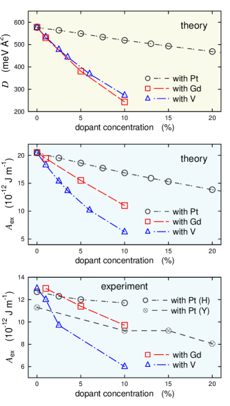
Figure 1: (Color online) Theoretical spin wave stiffness $D$ (upper panel) and exchange stiffness $A_{\text{ex}}$ (central panel) for Py doped with V, Gd, and Pt. Experimental values for $A_{\text{ex}}$ are shown in the lowermost panel, with the data from Ref. 5 for V-doped Py, from Ref. 6 for Gd-doped Py, and from Ref. 7 (circles) and Ref. 3 (circles with crosses) for Pt-doped Py.

Our focus is on comparing the trends of $D$ and $A_{\text{ex}}$ with the dopant concentration for different dopant types. This is inspected in Fig. 1. One can see that the spin wave stiffness $D$ for V-doped Py and Gd-doped Py is practically the same. The difference appears only for the exchange stiffness $A_{\text{ex}}$ and stems from the differences in the magnetization for these two systems (cf. the third columns of Tabs. 1 and 2). The experimental data are shown in the bottom graph of Fig. 1. Both experiment and theory suggest that the decrease of the exchange stiffness $A_{\text{ex}}$ with increasing dopant concentration is approximately linear and that this decrease is quickest for the V dopant and slowest for the Pt dopant.

Concerning the absolute values of $A_{\text{ex}}$, part of the difference between theory and experiment is due to the temperature effects. The theoretical data are for zero temperature. The experimental data were obtained by fitting the temperature-dependence of the magnetization to the Bloch law while assuming implicitly that the stiffness itself does not depend on temperature [5; 6; 7]. This is, however, not the case [27; 28; 29; 26] meaning that the experimental values for $A_{\text{ex}}$ in Fig. 1 correspond to an unknown effective temperature. Presumably the effect of this will not be very large: Temperature-dependent measurements of the spin wave stiffness of doped Py indicate that at room temperature the constant $D$ decreases to about 90 % of its zero-temperature value [26]. Therefore we assume that most of the difference in the absolute values of $A_{\text{ex}}$ as given by theory and by experiment comes from the spin wave stiffness constant $D$. Further comments are given at the beginning of Sec. IV below.

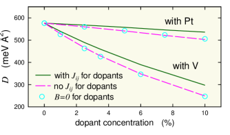
Figure 2: (Color online) Spin wave stiffness $D$ for Py doped with V and Pt calculated by considering the coupling constants $J_{ij}^{(\alpha\beta)}$ in Eqs. (7)–(8) for all atoms on the same footing (full lines), by completely ignoring the coupling constants for the dopants (dashed lines), and by additionally suppressing the exchange field $B$ for the dopant atoms (circles).

One of the intensively studied fundamental questions in connection with the spin dynamics of doped ferromagnets has been about the role of the magnetism of dopant atoms on the exchange and spin wave stiffness [3; 7]. We have shown already that the difference in the exchange stiffness $A_{\text{ex}}$ between V-doped and Gd-doped Py is because of the difference in the magnetization of these systems, which in turn stems from different magnetic moments at Gd and V atoms. We have also shown that for Gd doping it does not matter for $D$ whether the Gd moments are included in Eqs. (7)–(8) or not (Tab. 2). Let us now turn to the spin wave stiffness for Py doped with V and Pt, both of which are easy to polarize, and compare $D$ evaluated via two extreme approaches: (i) by treating the dopants equally as the host atoms concerning the coupling, i.e., both sums $\sum_{\alpha}$ in Eq. (7) and $\sum_{\beta}$ in Eq. (8) include also the dopant atoms, and (ii) by ignoring the coupling for the dopants altogether, i.e., neither of the sums $\sum_{\alpha}$ and $\sum_{\beta}$ includes the dopants. The difference between both approaches can be seen Fig. 2, where we display the results for Pt- and V-doping only; the data for Gd-doped Py are very similar to V-doped Py (cf. the upper panel of Fig. 1). One can see that even though ignoring the coupling for the dopants decreases the values of $D$ by up to 20 % (depending on the concentration), the overall trend and especially the difference between the effect of both dopants does not change. To proceed further, we performed another calculation where the effective local exchange field $B$ was suppressed for the Pt and V dopants. The results (depicted by the circles in Fig. 2) are nearly identical to the situation when the exchange coupling involving the dopant atoms is ignored.

We conclude from this that the polarizability of the dopants does not have a significant influence on the spin wave stiffness $D$ of doped permalloy. The reason why different dopants lead to different results for $D$ must be elsewhere, presumably in the details of the electronic structure and the related hybridization (see Sec. III.3 below).

III.2 Influence of dopants on the exchange coupling

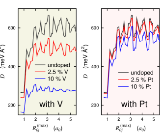
Figure 3: (Color online) Dependence of the stiffness constant $D$ on the maximum distance $R_{0j}^{\text{(max)}}$ accounted for when evaluating Eq. (8) for undoped permalloy and for permalloy doped by 2.5 % and 10 % of V (left) and Pt (right).

In the following we consider the mechanism through which different dopants affect the stiffness of permalloy. The first information concerns the size of the region which effectively determines the spin wave stiffness constant $D$. We mentioned already that to get good numerical stability, the sum over the sites $\sum_{j}$ in Eq. (8) has to include sites at very large distances $R_{0j}$ [9]. For a deeper insight, the dependence of the stiffness constant $D$ on the maximum distance $R_{0j}^{\text{(max)}}$ up to which the sum $\sum_{j}$ in Eq. (8) extends is presented in Fig. 3. No damping has been considered for simplicity ($\eta$=0). The constant $D$ oscillates with $R_{0j}^{\text{(max)}}$ and the amplitude of these oscillations decays very slowly. This is why the sum in Eq. (8) has to cover large distances $R_{0j}$ and why the damping factor $\eta$ has been introduced [9].

It is evident from Fig. 3 that significant variations of the spin wave stiffness constant $D$ only occur within few nearest shells — up to about 2$a_{0}$ ($a_{0}$ is the lattice constant). Afterwards, $D$ just oscillates around the mean value. If the difference in $D$ for two dopant concentrations is big for large $R_{0j}^{\text{(max)}}$, it is big also for small $R_{0j}^{\text{(max)}}$ and vice versa. The difference between V and Pt concerning the rate how $D$ decreases with increasing dopant concentration (see Fig. 1) is evident for small values of $R_{0j}^{\text{(max)}}$ already. Including large distances $R_{0j}$ when evaluating Eq. (8) is thus necessary just for technical reasons — to ensure the numerical stability.

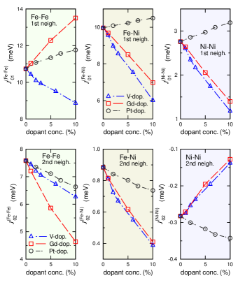
Figure 4: (Color online) Exchange coupling constants for Fe-Fe, Fe-Ni, and Ni-Ni atomic pairs if they are first nearest neighbors (upper panels) or second nearest neighbors (lower panels). Data for V-doped Py are shown by triangles, for Gd-doped Py by squares, and for Pt-doped Py by circles.

Further information how the nearest neighborhood affects the spin wave stiffness comes from the exchange coupling constants. Fig. 4 shows them for the (Fe-Fe), (Fe-Ni) and (Ni-Ni) pairs if they form the nearest neighbors and the next-nearest neighbors. Even though the stiffness constant $D$ has to be evaluated including also pairs whose members are much further apart, the main feature can be seen from $J_{01}$ and $J_{02}$ already: For the (Fe-Ni) and (Ni-Ni) pairs, the coupling constants for V-doped and Gd-doped Py are very similar whereas for Pt-doped Py they differ. As Ni has by far the highest concentration in our systems, this explains why the spin wave stiffness constant $D$ is similar for the V and Gd dopants and different for the Pt dopant.

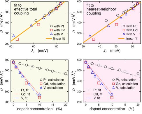
Figure 5: (Color online) Upper panels: Dependence of the theoretical spin wave stiffness $D$ on the effective exchange coupling parameter $J_{0}$ (left) and on the nearest-neighbor coupling $J_{1}$ (right). The markers denote calculated values of $D$, $J_{0}$, and $J_{1}$ for different dopants and concentrations, the straight lines show the linear fits. Lower panels: Calculated spin wave stiffness $D$ (markers) together with $D$ obtained from respective $J_{0}$ values relying on the linear $D(J_{0})$ fit (left) and from respective $J_{1}$ values relying on the $D(J_{1})$ fit (right).

Based on this, one can speculate that even though a formal evaluation of $D$ requires performing the sum $\sum_{j}$ in Eq. (8) up to a large distance $R_{0j}^{\text{(max)}}$, the bare influence of the doping might be accounted for by a more simple quantity. Let us first focus on the effective total coupling $J_{0}$ defined as

$$J_{0}\>=\>\sum_{j}J_{0j}\quad,$$ (9)

or, more specifically for our alloy system [cf. Eqs. (7)–(8)],

$$J_{0}\>=\>\sum_{\alpha}c_{\alpha}\sum_{j}\sum_{\beta}c_{\beta}J_{0j}^{(\alpha\beta)}\quad.$$ (10)

This quantity is related to the mean-field Curie temperature via

$$T_{C}^{\text{(MFA)}}\>=\>\frac{2}{3}\,\frac{1}{k_{\text{B}}}\,J_{0}\quad.$$

Note that for a translationally-periodic system, one does not need to perform the $\sum_{j}$-sum in Eq. (10) explicitly, the $J_{0}$ constant can be evaluated from the scattering paths operators in a similar way as the individual $J_{ij}$ constants [8].

The spin wave stiffness constant $D$ is plotted as a function of the effective total coupling $J_{0}$ (or, equivalently, $T_{C}^{\text{(MFA)}}$) in the upper left panel of Fig. 5. One can see that for Py doped with various impurities of different concentrations the dependence of $D$ on $J_{0}$ is nearly linear. Quantitatively it can be described by

$$D\>=\>79.6\,J_{0}\>-\>95$$ (11)

if $J_{0}$ is in meV and $D$ in meV Å². Using this universal fit, we can recover the dependence of $D$ on the concentration of the impurities by first evaluating $J_{0}$ for each system and then getting appropriate $D$ via Eq. (11). The outcome is shown in the lower left panel of Fig. 5. One can see that this model correctly separates the trends for the Pt impurity on the one side and for the V and Gd impurities on the other side and that the slope of the dependency of $D$ on the concentration is also reproduced quite well.

To simplify matters even more, one can ask whether the influence of impurities could be possibly described just by focusing on the nearest neighbors. Therefore we inspect the dependence of the stiffness constant $D$ on the effective coupling originating from the nearest neighbors only,

$$J_{1}\>=\>\sum_{\alpha}c_{\alpha}\,12\,\sum_{\beta}c_{\beta}J_{01}^{(\alpha\beta)}\quad.$$ (12)

The constant $J_{01}^{(\alpha\beta)}$ characterizes the exchange coupling between the central atom of type $\alpha$ and an atom of type $\beta$ in the first coordination shell and the factor 12 stands for the number of nearest neighbor sites for the fcc lattice. The resulting dependence of $D$ on $J_{1}$ is shown in the upper right panel of Fig. 5. The spread around the linear fit

$$D\>=\>109.4\,J_{1}\>-\>118$$ (13)

is now bigger than in the case of the $D(J_{0})$ dependence but still quite small. Indeed, by relying on Eq. (13), one can get the dependence of $D$ on the impurity concentration with a similar accuracy as by relying on Eq. (11) — compare the lower right panel of Fig. 5 with the lower left panel of the same figure. One could thus say that the trend of the spin wave stiffness with the dopant concentration is, to a decisive degree, determined by the coupling between the nearest neighbors. As concerns the value of the stiffness constant $D$, it depends on the interaction within few nearest shells — see Fig. 3 and the related text at the beginning of Sec. III.2.

III.3 Influence of dopants on the electronic structure

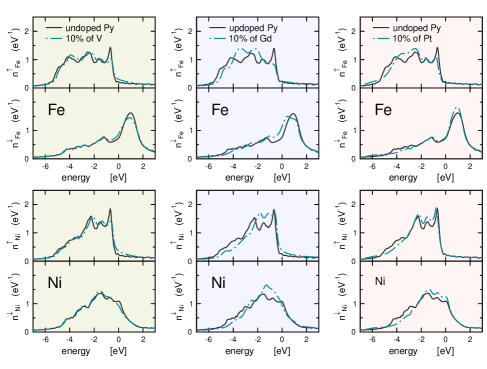
Figure 6: (Color online) Upper panels: Comparison of the DOS for Fe atoms in undoped Py and in Py doped by 10 % of V (left), Gd (center), and Pt (right). Lower panels: As in the upper panels but for Ni atoms.

The next step is to inspect the electronic structure. The changes in the DOS for the Fe and Ni atoms caused by the doping can be seen in Fig. 6, where we show in the same graphs the data for undoped Py and for Py doped by 10 % of V, Gd, and Pt. For the V dopant the changes are minimal: the corresponding DOS curves are hardly distinguishable from each other. For the Pt dopant, the changes are more significant. Still larger but as a whole similar changes can be observed also for the Gd dopant. Based on Fig. 6, one would infer that the hybridization between the electronic states of the host and of the dopant is largest for the Gd dopant and smallest for the V dopant.

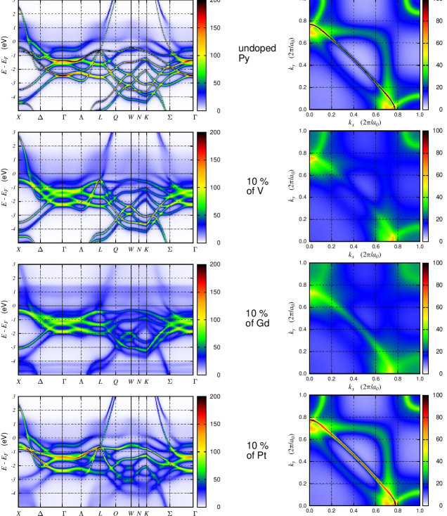
Figure 7: (Color online) Comparison of Bloch spectral functions for undoped Py and for Py doped by 10 % of V, Gd, and Pt.

Reckoning the results discussed so far, there seems to be a difference in the picture offered by inspecting the $J_{ij}$ constants in Fig. 4 and by inspecting the DOS in Fig. 6. The analysis of the coupling constants suggests that the V and Gd dopants have a similar effect on the electronic structure (which determines the $J_{ij}$’s) whereas the influence of the Pt dopant is different. This follows also from spin wave stiffness $D$ shown in Fig. 1. On the other hand, the analysis of the DOS suggests that qualitatively similar effects should follow from introducing the Gd and Pt dopants whereas it is the V dopant which differs in its effect on the electronic structure of permalloy.

A more thorough view on the electronic structure of alloys is provided by the Bloch spectral function $A(\bm{k},E)$, which can be viewed as a $\bm{k}$-resolved DOS. The effect of introducing 10 % of V, Gd, and Pt into Py is shown in Fig. 7. Left panels show $A(\bm{k},E)$ when the $\bm{k}$ vector is varied along straight lines connecting high-symmetry points in the first Brillouin zone, right panels show the Bloch spectral function at the Fermi level $A(\bm{k},E_{F})$ when the $\bm{k}$ vector spans a two-dimensional section of the $\bm{k}$-space (keeping $k_{z}$=0). By observing the $E-\bm{k}$ scans, one cannot say unambiguously which dopant introduces largest changes to the electronic structure of permalloy. E.g., around the $\Gamma$ point the smallest changes to $A(\bm{k},E)$ are for the Pt dopant while changes introduced by V or Gd doping are larger. On the other hand, if one focuses on the region around the $N$ point, doping by Gd has the largest impact whereas by V the smallest impact. However, when discussing the spin wave stiffness, one has to keep on mind that it is associated with changes of electron energy caused by spin wave excitations characterized by small wave vector $\bm{q}$, and therefore contributed mainly by the electronic states close to the Fermi level $E_{F}$. As a result, the spin wave stiffness is sensitive first of all to the electronic structure around $E_{F}$. The impact of doping on the states around $E_{F}$ is illustrated in the right panels of Fig. 7. Here one can see that the changes introduced by doping by Pt are significantly smaller than changes introduced by doping by V or Gd.

Table 5: Integrals of the differences of Bloch spectral functions at $E_{F}$ for doped and undoped systems, as defined in Eq. 14. The units are arbitratry.

dopant	concentration	concentration
type	1%	10%
V	$4.49$	$20.18$
Gd	$6.07$	$26.52$
Pt	$1.38$	$7.62$

The influence of the doping on the electronic structure around $E_{F}$ can be quantified by integrating the difference of Bloch spectral functions for a doped system and for an undoped system. We evaluated the integral

$$\int\!\mathrm{d}k\>\left|A_{\text{X}}(\bm{k},E_{F})\,-\,A_{\text{undoped}}(\bm{k},E_{F})\right|\quad,$$ (14)

where $A_{\text{X}}(\bm{k},E_{F})$ and $A_{\text{undoped}}(\bm{k},E_{F})$ are the Bloch spectral functions for doped and undoped systems, respectively, and the integration is carried along the path $X$-$\Delta$-$\Gamma$-$\Lambda$-$L$-$Q$-$W$-$N$-$K$-$\Sigma$-$\Gamma$ outlined at the horizontal axes of the left graphs in Fig. 7. The results are shown in Tab. 5 for two dopant concentrations. The largest changes in the electronic structure are introduced by Gd doping followed by still considerable changes introduced by V doping, while the changes introduced by Pt are small.

The picture emerging from analyzing Bloch spectra function is thus different from the picture offered by the DOS. The smallest changes in $A(\bm{k},E)$ with respect to undoped Py are clearly for the Pt dopant. The changes introduced by V or Gd doping are bigger. Based on Fig. 7 and Tab. 5 one would assess that the changes in the electronic structure introduced by doping Py with Pt are significantly smaller than the changes introduced by doping Py with V or Gd. Intuitively, this implies that for the Pt dopant the changes in the values of $D$ will be smaller than for the V or Gd dopants — in agreement with the results presented in Sec. III.1. The Bloch spectral function thus offers a more reliable picture than the DOS.

IV Discussion

Ab-initio calculations reproduce the experiment both as concerns the dependence of $A_{\text{ex}}$ on the chemical type of the dopant and as concerns the dependence of $A_{\text{ex}}$ on the dopant concentration. Regarding the absolute numbers, there are some differences, both between our theory and experiment and between our theory and earlier calculations. In particular our value of the spin wave stiffness $D$ for undoped permalloy Fe₁₉Ni₈₁ of 576 meV Å² is higher than 515 meV Å² obtained by Yu et al. [30] via the tight-binding linear muffin-tin orbital method or 522 meV Å² obtained by Pan et al. [4] via the KKR-Green’s function method. The reason for this is unclear, let us just note that several convergence issues have to be addressed when evaluating $D$; our settings are given in Sec. II.2. Recent experimental values for $D$ of Py are 390 meV Å² [31] and 440 meV Å² [26], i.e., less than the theoretical values. This is probably linked to problems with describing the exchange coupling of Ni in terms of the coupling constants $J_{ij}$ — there is an even larger difference between theory and experiment for $D$ of fcc Ni [9; 30]. Besides, the difference between our values for $A_{\text{ex}}$ and the experiment is probably affected also by the temperature-dependence of $D$, which affects the interpretation of some experiments (as mentioned in Sec. III.1). Another factor not accounted for by our calculations and possibly affecting the comparison between theory and experiment is the polycrystallinity of the experimental samples that were prepared by sputtering [3; 5; 6; 7]. One should acknowledge that there may be problems also at the experimental side as the spread of values available in the literature is quite large. A critical assessment would require a standalone study. We just note for illustration that, e.g., in the case of Fe the available experimental data for $D$ include 270 meV Å² [32] as well as 307 meV Å² [33], in the case of Ni 398 meV Å² [34] as well as 530 meV Å² [31], and in the case of Py 335 meV Å² [35] as well as 390 meV Å² [31]. The differences between experimental values of $A_{\text{ex}}$ for Pt-doped permalloy reported by Hrabec et al. [7] and by Yin et al. [3] (cf. Fig. 1) are thus not unusual. Let us summarize that that discrepancies between theory and experiment are often observed for the spin wave and/or exchange stiffness and, so far, they are not fully understood.

The fact that the spin wave stiffness $D$ and the exchange stiffness $A_{\text{ex}}$ are related through magnetization [see Eq. (2)] which itself is affected by the doping means that there may be situations where doping by two different materials will lead to a similar $D$ but a different $A_{\text{ex}}$ (or vice versa). In particular we found that the spin wave stiffness $D$ for V-doped Py and Gd-doped Py is very similar but there is a difference in the exchange stiffness $A_{\text{ex}}$ which arises just from the difference in the magnetization (cf. Fig. 1).

The influence of doping on the stiffness $D$ can be discussed just by considering the influence of the atoms in the first coordination shell (Fig. 5). This might appear as surprising reckoning the slow convergence of the sums in Eqs. (5) or (8) [9]. The explanation might be that what we investigate in Fig. 5 is just the variation of $D$ with the doping. Eq. (13), which we used for our analysis, was derived by fitting the $D(J_{1})$ dependence relying on the values of $D$ evaluated by extending the $\sum_{j}$-sum to the interatomic distance as large as 20.5 $a_{0}$. However, once the fit according to Eq. (13) has been established, one can predict how the doping will influence the stiffness $D$ just by considering the nearest-neighbors coupling. Our fit has been verified for three quite different dopants so presumably it can be used to assess the effect of doping by other elements as well. This can be helpful in current efforts to manipulate spin-driven properties of materials.

Our results indicate that it does not really matter whether the exchange coupling between the host atoms and the dopant atoms is included in the stiffness calculation or not; the values of $D$ are by about 5 % smaller in the latter case but the trends are very similar (see Tab. 2 and Fig. 2). This indicates that neither the polarizability of the dopant nor the exchange coupling between the dopant atoms and the host atoms are decisive factors for the spin wave stiffness $D$ (unlike what was conjectured before, see for example Refs. [3; 7]). The hybridization between the host states and the dopant states (or lack of it) is more important than the dopant polarizability. Interestingly, this hybridization has to be assessed not from the DOS — which contains only a limited information — but from the Bloch spectral function (cf. Figs. 6 and 7). The fact that inspecting the Bloch spectra function provides a better insight than inspecting the DOS alone can be seen as a demonstration that the exchange coupling constants $J_{ij}$ reflect the full electronic structure, including its $\bm{k}$-dependence.

Earlier studies indicated that the exchange coupling in 4$f$-electron systems cannot be properly described within the local density approximation or the GGA. Employing the open core formalism was suggested and tested for this purpose [23]. In our case we found, nevertheless, that the stiffness of Gd-doped Py calculated within the open-core formalism and within the GGA is very similar. The reason for this might be that as the Gd atoms are here just impurities, their $f$ electrons are localized “naturally”, by the lack of their hybridization with the host states. A further reduction of the hybridization of the Gd $f$ states via the open core formalism is thus not needed.

Like most other calculations of the spin wave and exchange stiffness we rely on the ASA [2; 3; 4; 9]. For close-packed metallic systems such as those we are studying here this is not a serious limitation. This was demonstrated, e.g., on a study of magnetic properties of disordered FePt where the CPA was applied both within the ASA and within a full-potential scheme [36].

V Conclusions

Ab-initio calculations for doped permalloy indicate that the exchange stiffness constant $A_{\text{ex}}$ decreases with increasing dopant concentration. This decrease is most rapid for the V dopant followed by the Gd dopant, the slowest decrease is for the Pt dopant — in agreement with experiment. The influence of the V-doping and the Gd-doping on the spin wave stiffness $D$ is very similar, the difference in the influence of the doping on the exchange stiffness $A_{\text{ex}}$ comes from the differences in the magnetization $M_{s}$ for V-doped and Gd-doped Py. The rate of change of the spin wave stiffness upon introducing the dopants can be discussed by just considering the influence of the atoms in the first coordination shell. The hybridization between impurity and host states is more important for the stiffness than the polarizability of the impurity.

*

Appendix A Accuracy of $\lim_{\eta\rightarrow 0}D(\eta)$ extrapolation

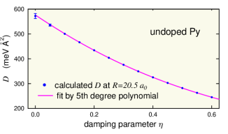
Figure 8: (Color online) Spin wave stiffness constant $D(\eta)$ for undoped Py evaluated by performing the summation in Eq. (8) up to $R_{0j}^{\text{(max)}}=20.5a_{0}$ ($a_{0}$ is the lattice constant) for several values of the damping parameter $\eta$ together with the fifth-degree polynomial used to extrapolate the data to zero damping.

The values of the spin wave stiffness $D$ presented in this paper rely on extrapolating data evaluated according to Eqs. (7)–(8) for finite values of the damping parameter $\eta$ down to $\eta=0$. This may be a tricky procedure. To present an analysis of all its aspects would be beyond the scope of this paper but the accuracy of our data can be illustrated on the case of undoped Py. Fig. 8 displays original $D(\eta)$ data points together with the fifth-degree polynomial used for the $\eta\rightarrow 0$ extrapolation. The $D$ constant obtained without any damping ($\eta=0$) is shown as well. The errorbars depict errors caused by not yet fully damped $D(R)$ oscillations; they are discernible only for $\eta>0.1$ at this scale. The extrapolating polynomial was found by a least-squares fit within the interval $\eta\in[0.15;1.00]$. One can see that the fit describes very well also the datapoints for $\eta=0.10$, $\eta=0.05$, and $\eta=0.00$ (within the numerical accuracy given by the $D(R)$ oscillations which are damped more and more as $\eta$ increases). If the V, Gd, or Pt dopants are introduced, the procedure becomes even more robust: namely, further increase of the disorder increases the damping of the $D(R)$ oscillations and the values of $D$ thus become numerically more stable.

The extrapolation is not a unambiguous procedure. One can always speculate about using a polynomial of a different degree for the fit or about varying a bit the interval of the $\eta$ values for which the polynomial is fitted. Within these limits, the numerical accuracy of our values of $D$ is few units of meV Å². This is sufficient for our purpose, especially given the fact that our focus is on the trends of the $D$ values evaluated always according to the same recipe.

References

- Vaz et al. [2008] C. A. F. Vaz, J. A. C. Bland, and G. Lauhoff, Rep. Prog. Phys. 71, 056501 (2008).
- Kübler [2000] J. Kübler, Theory of Itinerant Electron Magnetism, International Series of Monographs on Physics (Oxford University Press, Oxford, 2000).
- Yin et al. [2015] Y. Yin, F. Pan, M. Ahlberg, M. Ranjbar, P. Dürrenfeld, A. Houshang, M. Haidar, L. Bergqvist, Y. Zhai, R. K. Dumas, A. Delin, and J. Åkerman, Phys. Rev. B 92, 024427 (2015).
- Pan et al. [2016] F. Pan, J. Chico, J. Hellsvik, A. Delin, A. Bergman, and L. Bergqvist, Phys. Rev. B 94, 214410 (2016).
- Lepadatu et al. [2010a] S. Lepadatu, J. S. Claydon, C. J. Kinane, T. R. Charlton, S. Langridge, A. Potenza, S. S. Dhesi, P. S. Keatley, R. J. Hicken, B. J. Hickey, and C. H. Marrows, Phys. Rev. B 81, 020413(R) (2010a).
- Lepadatu et al. [2010b] S. Lepadatu, J. S. Claydon, D. Ciudad, C. J. Kinane, S. Langridge, S. S. Dhesi, and C. H. Marrows, Appl. Physics Lett. 97, 072507 (2010b).
- Hrabec et al. [2016] A. Hrabec, F. J. T. Gonçalves, C. S. Spencer, E. Arenholz, A. T. N’Diaye, R. L. Stamps, and C. H. Marrows, Phys. Rev. B 93, 014432 (2016).
- Liechtenstein et al. [1987] A. I. Liechtenstein, M. I. Katsnelson, V. P. Antropov, and V. A. Gubanov, J. Magn. Magn. Materials 67, 65 (1987).
- Pajda et al. [2001] M. Pajda, J. Kudrnovský, I. Turek, V. Drchal, and P. Bruno, Phys. Rev. B 64, 174402 (2001).
- Thoene et al. [2009] J. Thoene, S. Chadov, G. Fecher, C. Felser, and J. Kübler, J. Phys. D: Appl. Phys. 42, 084013 (2009).
- Dürrenfeld et al. [2015] P. Dürrenfeld, F. Gerhard, J. Chico, R. K. Dumas, M. Ranjbar, A. Bergman, L. Bergqvist, A. Delin, C. Gould, L. W. Molenkamp, and J. Åkerman, Phys. Rev. B 92, 214424 (2015).
- Mryasov et al. [2005] O. N. Mryasov, U. Nowak, K. Y. Guslienko, and R. W. Chantrell, Europhys. Lett. 69, 805 (2005).
- Mryasov [2005] O. N. Mryasov, Phase Transitions 78, 197 (2005).
- Ležaić et al. [2006] M. Ležaić, P. Mavropoulos, J. Enkovaara, G. Bihlmayer, and S. Blügel, Phys. Rev. Lett. 97, 026404 (2006).
- Polesya et al. [2010] S. Polesya, S. Mankovsky, O. Šipr, W. Meindl, C. Strunk, and H. Ebert, Phys. Rev. B 82, 214409 (2010).
- Nibarger et al. [2003] J. P. Nibarger, R. Lopusnik, Z. Celinski, and T. J. Silva, Appl. Physics Lett. 83, 93 (2003).
- Shaw et al. [2013] J. M. Shaw, H. T. Nembach, T. J. Silva, and C. T. Boone, J. Appl. Phys. 114, 243906 (2013).
- Ebert et al. [2011] H. Ebert, D. Ködderitzsch, and J. Minár, Rep. Prog. Phys. 74, 096501 (2011).
- Ebert [2014] H. Ebert, The sprkkr package version 7, http://olymp.cup.uni-muenchen.de/ak/ebert/SPRKKR (2014).
- Kudrnovský and Drchal [1990] J. Kudrnovský and V. Drchal, Phys. Rev. B 41, 7515 (1990).
- Carva et al. [2016] K. Carva, J. Kudrnovský, F. Máca, V. Drchal, I. Turek, P. Baláž, V. Tkáč, V. Holý, V. Sechovský, and J. Honolka, Phys. Rev. B 93, 214409 (2016).
- Richter [2001] M. Richter, in Handbook of Magnetic Materials, Vol. 13, edited by K. H. J. Buschow (North-Holland, Amsterdam, 2001) pp. 87–228.
- Turek et al. [2003] I. Turek, J. Kudrnovský, G. Bihlmayer, and S. Blügel, J. Phys.: Condens. Matter 15, 2771 (2003).
- Rusz et al. [2005] J. Rusz, I. Turek, and M. Diviš, Phys. Rev. B 71, 174408 (2005).
- Khmelevskyi et al. [2007] S. Khmelevskyi, T. Khmelevska, A. V. Ruban, and P. Mohn, J. Phys.: Condens. Matter 19, 326218 (2007).
- Yin et al. [2017] Y. Yin, M. Ahlberg, P. Dürrenfeld, Y. Zhai, R. K. Dumas, and J. Åkerman, IEEE Magnetics Letters 8, 1 (2017).
- Mathon and Wohlfarth [1968] J. Mathon and E. P. Wohlfarth, Proc. Roy. Soc. (London) A 302, 409 (1968).
- Riedi [1977] P. Riedi, Physica B+C 91, 43 (1977).
- Kaul and Babu [1994] S. N. Kaul and P. D. Babu, Phys. Rev. B 50, 9308 (1994).
- Yu et al. [2008] P. Yu, X. F. Jin, J. Kudrnovský, D. S. Wang, and P. Bruno, Phys. Rev. B 77, 054431 (2008).
- Nakai [1983] I. Nakai, J. Phys. Soc. Jpn. 52, 1781 (1983).
- Pauthenet [1982] R. Pauthenet, J. Appl. Phys. 53, 2029 (1982).
- Loong et al. [1984] C. Loong, J. M. Carpenter, J. W. Lynn, R. A. Robinson, and H. A. Mook, J. Appl. Phys. 55, 1895 (1984).
- Mitchell and Paul [1985] P. W. Mitchell and D. M. Paul, Phys. Rev. B 32, 3272 (1985).
- Hennion et al. [1975] M. Hennion, B. Hennion, A. Castets, and D. Tocchetti, Solid State Commun. 17, 899 (1975).
- Khan et al. [2017] S. A. Khan, J. Minár, H. Ebert, P. Blaha, and O. Šipr, Phys. Rev. B 95, 014408 (2017).