More on the universal equation for Efimov states

Abstract

Efimov states are a sequence of shallow three-body bound states that arise when the two-body scattering length is much larger than the range of the interaction. The binding energies of these states are described as a function of the scattering length and one three-body parameter by a transcendental equation involving a universal function of one angular variable. We provide an accurate and convenient parametrization of this function. Moreover, we discuss the effective treatment of range corrections in the universal equation and compare with a strictly perturbative scheme.

I Introduction

The interactions of nonrelativistic particles with short-range interactions at extremely low energies are determined primarily by their $S$-wave scattering length $a$. If $|a|$ is much larger than the characteristic range $l$ of their interaction, low-energy atoms exhibit universal properties that are insensitive to the details of the interaction potential Braaten:2004rn . In the two-body sector, $a$ is the only relevant dimensionful parameter at low energies and all observables simply scale with appropriate powers of $a$. If $a>0$, there is one shallow two-body bound state (the dimer) with binding energy $E_{2}=\hbar^{2}/ma^{2}$. In the three-body sector, the universal properties were first deduced by Efimov Efi71 . The most remarkable is the existence of a sequence of three-body bound states with binding energies $E_{3}^{(n)}$ geometrically spaced in the interval between $\hbar^{2}/(ma^{2})$ and $\hbar^{2}/(ml^{2})$. The number of these “Efimov states” is roughly $\ln(|a|/l)/\pi$ if $|a|$ is large enough. In the limit $|a|\to\infty$, there is an accumulation of infinitely many Efimov states at threshold (the “Efimov effect”). The knowledge of their binding energies is essential for understanding the energy dependence of low-energy three-body observables. For example, Efimov states can have dramatic effects on atom-dimer scattering if $a>0$ Efi71 ; BHK99 and on three-body recombination if $a<0$ EGB99 ; BBH00 .

A large two-body scattering length can be obtained by fine-tuning a parameter in the interatomic potential to bring a real or virtual two-body state close to threshold. The fine tuning can be provided accidentally by nature. An example is the ⁴He atom, whose scattering length $a=104$ Å Gri00 is much larger than the effective range $l\approx 7$ Å. There are two ⁴He trimer states, the ground state state Sch94 where range corrections are significant, and the recently observed excited state which is almost an ideal Efimov state Kun15 . For atoms the fine tuning can also be obtained by using Feshbach resonances Chi10 . The scattering length of alkali atoms can be changed experimentally by tuning an external magnetic field. An important difference from He is that the interatomic potentials of alkali atoms support many deep two-body bound states. Using Feshbach resonances, Efimov states have been observed in a variety of atoms including ¹³³Cs, ⁶Li, ⁷Li, and several mixtures of atoms (see Refs. Bra07 ; Naidon:2016dpf for reviews).

Efimov’s universal equation for the energies $E_{3}^{(n)}$ follows from the approximate scale-invariance at length scales $R$ in the region $l\ll R\ll|a|$ and the conservation of probability. Introducing polar variables $H$ and $\xi$ in the plane defined by the variables $1/a$ and $K={\rm sgn}(E)|mE|^{1/2}/\hbar$, the binding energies of the Efimov states are solutions to a transcendental equation involving a single universal function $\Delta(\xi)$ of $\xi$ Efi71 . In Ref. Braaten:2002sr , this equation was extended to the case where deeply bound dimers are present by introducing a loss parameter $\eta_{*}$.

Here, we restrict ourselves to the case without deep dimers and consider the equation for the radial wave function $f(R)$ in the adiabatic hyperspherical representation of the three-body problem Jen93 ; Nie01 . The hyperspherical radius for three identical bosons with coordinates ${\bf r}_{1}$, ${\bf r}_{2}$, and ${\bf r}_{3}$ is $R^{2}=(r_{12}^{2}+r_{13}^{2}+r_{23}^{2})/3$, where $r_{ij}=|{\bf r}_{i}-{\bf r}_{j}|$. If $|a|\gg l$, the radial equation for 3 bosons with total angular momentum zero reduces in the region $l\ll R\ll|a|$ to

$$-{\hbar^{2}\over 2m}\left[{\partial^{2}\over\partial R^{2}}+{s_{0}^{2}+1/4\over R^{2}}\right]f(R)=Ef(R),$$ (3)

where $s_{0}\approx 1.00624$. This has the same form as the one-dimensional Schrödinger equation for a particle in an attractive $1/R^{2}$ potential. If we impose a boundary condition on $f(R)$ at short-distances of order $l$, the radial equation (3) has solutions at discrete negative values of the eigenvalue $E=-E_{3}^{(n)}$, with $E_{3}^{(n)}$ ranging from order $\hbar^{2}/(ml^{2})$ to order $\hbar^{2}/(ma^{2})$. The corresponding eigenstates are called Efimov states. As $|a|\to\infty$, their spectrum approaches the simple law $E_{3}^{(n)}/E_{3}^{(n+1)}=e^{2\pi/s_{0}}\approx 515\,$.

Efimov’s equation can be derived by constructing a solution to Eq. (3) in the region $l\ll R\ll|a|$. We define the radial variable $H$ and the angular variable $\xi$ via

$$H^{2}=mE_{3}^{(n)}/\hbar^{2}+1/a^{2}\,\qquad\mbox{ and }\qquad\tan\xi=-a\sqrt{mE_{3}^{(n)}}/\hbar\,.$$ (4)

These variables are illustrated in Fig. 1 together with the general form of the Efimov spectrum in the $1/a-K$ plane.

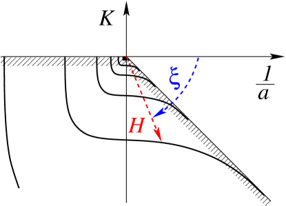
Figure 1: Illustration of the Efimov spectrum in the $1/a-K$ plane. The solid lines indicate the Efimov states, while the hashed areas give the scattering thresholds. The new variables $H$ and $\xi$ are illustrated by the dashed lines.

Since we are interested in low energies $mE_{3}^{(n)}/\hbar^{2}\sim 1/a$, the energy eigenvalue in (3) can be neglected. The most general solution is a superposition of outgoing and incoming hyperspherical waves Efi71 ,

$$f(R)=\sqrt{HR}\left[Ae^{is_{0}\ln(HR)}+Be^{-is_{0}\ln(HR)}\right],$$ (5)

where the dimensionless coefficients $A$ and $B$ can depend on $\xi$. At shorter distances $R\sim l$ and longer distances $R\sim|a|$, the wavefunction is more complicated, but a solution in this region is not required because of unitarity Efi71 .

We first consider the short-distance region. If there are no deep two-body bound states with binding energies $E_{2}\gg\hbar^{2}/(ma^{2})$, the two-body potential supports no bound states at all if $a<0$ and only the shallow dimer with binding energy $E_{2}=\hbar^{2}/(ma^{2})$ if $a>0$. The probability in the incoming wave must then be fully reflected at short distances and we can set $B=Ae^{i\theta}$. The phase $\theta$ can be specified by giving the logarithmic derivative of the radial wave function, $R_{0}f^{\prime}(R_{0})/f(R_{0})$, at any point $l\ll R_{0}\ll|a|$. The resulting expression for $\theta$ has a simple dependence on $H$:

$$\theta/2 = s_{0}\ln(H/c\kappa_{*})\,.$$ (6)

The quantity $c\kappa_{*}$ is a complicated function of $R_{0}$ and $R_{0}f^{\prime}(R_{0})/f(R_{0})$. It differs by an unknown constant $c$ from the three-body parameter $\kappa_{*}$ defined by Eq. (7) below.

We next consider large distances $R\sim|a|$. In general, an outgoing hyperspherical wave incident on the $R\sim|a|$ region can either be reflected or else transmitted to $R\to\infty$ as a scattering state. For bound states in the region $-\pi<\xi<-\pi/4$, the probability must be totally reflected such that $B=Ae^{i\Delta(\xi)}$, where the phase $\Delta$ depends on the angle $\xi$. Compatibility with the constraint from short distances requires $\theta=\Delta(\xi)\;{\rm mod}\;2\pi$. Using Eq. (6) for $\theta$ and inserting the expression for $H$, we obtain Efimov’s equation Efi71

$$E^{(n)}_{3}+{\hbar^{2}\over ma^{2}}=\frac{\hbar^{2}\kappa_{*}^{2}}{m}\,e^{-2\pi n/s_{0}}\exp\left[\Delta\left(\xi\right)/s_{0}\right]\,,$$ (7)

where the constant $c$ was absorbed into $\Delta(\xi)$ such that $\Delta(-\pi/2)\equiv 0$. This convention is used throughout the paper. Note that we measure $E_{3}$ from the three-boson threshold. $\kappa_{*}$ is thus the binding momentum of the state with label $n=0$ in the unitary limit. Once the universal function $\Delta(\xi)$ is known, the Efimov energies $E^{(n)}_{3}$ can be calculated by solving Eq. (7) for different integers $n$. This equation has an exact discrete scaling symmetry: if there is an Efimov state with binding energy $E^{(n)}_{3}$ for the parameters $a$ and $\kappa_{*}$, then there is also an Efimov state with binding energy $\lambda^{2}E^{(n)}_{3}$ for the parameters $\lambda^{-1}a$ and $\kappa_{*}$ if $\lambda=e^{k\pi/s_{0}}$ with $k$ an integer.

Equivalently, Eq. (7) can be written in parametric form as Kievsky:2012ss

$$\frac{E_{3}^{(n)}\,ma^{2}}{\hbar^{2}}=\tan^{2}\xi\,,\qquad\qquad\kappa_{*}a=e^{n\pi/s_{0}}\frac{e^{-\Delta\left(\xi\right)/(2s_{0})}}{\cos\xi}\,.$$ (8)

This form can be generalized straightforwardly to include range corrections but the universal function $\Delta(\xi)$ remains the same. $\Delta(\xi)$ can be calculated by solving the three-body problem for the Efimov binding energies in various potentials whose scattering lengths are so large that effective range corrections are negligible or by solving the Skorniakov-Ter-Martirosian integral equations for the zero-range case STM57 ; Braaten:2004rn .

II Universal Function $\Delta(\xi)$

An explicit parametrization of the universal function $\Delta\left(\xi\right)$ was first extracted from solutions of the zero-range STM equations derived from effective field theory in Refs. Braaten:2002sr ; Braaten:2004rn . We start by revisiting the parametrization from Braaten:2004rn , which has the general form

$$\Delta(\xi)=P_{f}^{(n)}\left(\xi\right)\equiv\sum_{k=0}^{n}c_{k}\cdot\left(f\left(\xi\right)\right)^{k}\,.$$ (9)

The parametrization was given separately for the three intervals $-\frac{3\pi}{8}<\xi\leq-\frac{\pi}{4}$, $-\frac{5\pi}{8}<\xi\leq-\frac{3\pi}{8}$, and $-\pi\leq\xi\leq-\frac{5\pi}{8}$. It reads

$$\Delta(\xi) =\begin{cases}3.10\,f_{1}(\xi)^{2}-9.63\,f_{1}(\xi)+6.04\,,&-\frac{3\pi}{8}<\xi\leq-\frac{\pi}{4}\,,\\ 1.17\,f_{2}(\xi)^{3}+1.97\,f_{2}(\xi)^{2}+2.12\,f_{2}(\xi)\,,&-\frac{5\pi}{8}<\xi\leq-\frac{3\pi}{8}\,,\\ 0.25\,f_{3}(\xi)^{2}+0.28\,f_{3}(\xi)-0.89\,,&-\pi\leq\xi\leq-\frac{5\pi}{8}\,,\end{cases}$$ (10)

where

$$f_{1}\left(\xi\right) =\sqrt{-\frac{\pi}{4}-\xi},$$ (11)

$$f_{2}\left(\xi\right) =\frac{\pi}{2}+\xi,$$ (12)

$$f_{3}\left(\xi\right) =\left(\pi+\xi\right)^{2}\cdot\exp\left(-\left(\pi+\xi\right)^{-2}\right)\,.$$ (13)

In the left panel of Fig. 2, we show the parametrization of Eq. (10) together with an shifted version of the original data set $\mathbb{O}$, which consists of 31 data pairs $(\xi,\Delta(\xi))$ in total. The data are well captured by this parametrization.

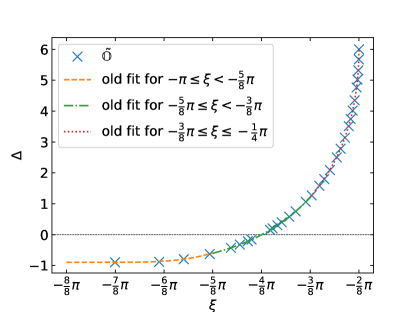
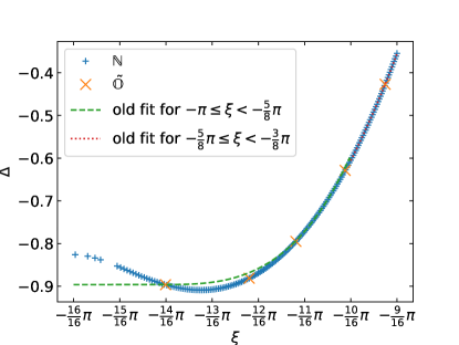
Figure 2: Left panel: parametrization (10) with old data set from Braaten:2002sr , which was shifted approximately by 8.214 in order to use the same convention as Braaten:2004rn . Right panel: parametrization (10) with shifted old data set $\tilde{\mathbb{O}}$ and new data set $\mathbb{N}$ in the region $\xi\hskip 1.99997pt\raisebox{2.15277pt}{$>$}\raisebox{-3.00003pt}{$\sim$}\hskip 1.99997pt-\pi$.

We have obtained a new set of binding energies $E_{3}$ as a function of the inverse scattering length $1/a$ by numerically solving the STM integral equation with a cutoff in momentum space STM57 . In particular, we take Eq. (340) of Ref. Braaten:2004rn for $H(\Lambda)=0$,

$${\cal B}(p)=\frac{4}{\pi}\int_{0}^{\Lambda}dq\,q^{2}\left[\frac{1}{2pq}\ln\frac{p^{2}+pq+q^{2}-E_{3}-i\epsilon}{p^{2}-pq+q^{2}-E_{3}-i\epsilon}\right]\left[-\frac{1}{a}+\sqrt{\frac{3q^{2}}{4}-E_{3}-i\epsilon}\right]^{-1}{\cal B}(q)\,,$$ (14)

where ${\cal B}(p)$ gives the residue at the pole of particle-dimer scattering amplitude at the trimer energy $E_{3}$, and $\Lambda$ is the cutoff. In principle there is an additional three-body term $H(\Lambda)$ with log-periodic behaviour imposed by discrete scale invariance BHK99 . In the present calculations we just set it to zero; by doing so, the cutoff $\Lambda$ plays the role of the three-body parameter Khar73 ; Hammer:2000nf . Thus $\Lambda$ is the scale that fixes the energies, $E_{3}=\hbar^{2}\kappa^{2}/m\Lambda^{2}$, and the lengths, $a=\tilde{a}/\Lambda$. To get rid of the finite cutoff effects, we need to consider high excited states; in the present calculations we have calculated the second excited state.

In order to numerically solve Eq. (14), we have chosen a grid for the values of the dimensionless momenta, $q/\Lambda$ and $p/\Lambda$, turning Eq. (14) into an eigenvalue problem

$${\cal B}={\cal I}(\kappa^{2}){\cal B}$$ (15)

for the matrix ${\cal I}(\kappa^{2})$ which is a function of the three-body energy $E_{3}=\hbar^{2}\kappa^{2}/m\Lambda^{2}$; the value sought for the trimer energy is that for which the eigenvalue is equal to one.

In Table 1, we report our values of the binding momentum $\kappa_{*}$ at the unitary point, our values of scattering lengths at the three-particle, $\kappa_{*}a_{-}$, and particle-dimer, $\kappa_{*}a_{*}$, thresholds in units of $\kappa_{*}$ for the first few states together with the ratio of the momenta. To assess the accuracy of our calculation, we compare our values with the theoretical prediction of Refs. Gogolin:2008xx ; Braaten:2004rn .

Level	$\kappa_{*}^{(n)}$	$\kappa_{*}^{(n)}/\kappa_{*}^{(n+1)}$	$\kappa_{*}^{(n)}a_{-}^{(n)}$	$\kappa_{*}^{(n)}a_{*}^{(n)}$
0	$1.7793756\cdot 10^{-1}$	22.9310	-1.4485	0.055336
1	$7.7597079\cdot 10^{-3}$	22.6948	-1.5044	0.073710
2	$3.4191512\cdot 10^{-4}$	22.6940	-1.5069	0.070907
3	$1.5066314\cdot 10^{-5}$
$\vdots$	$\vdots$	$\vdots$	$\vdots$	$\vdots$
$\infty$	0	22.69438	-1.50763 Gogolin:2008xx	0.07076 Braaten:2004rn

Table 1: Some special values obtained by numerically solving Eq. (14).

The new data set contains 5029 pairs $(1/a,E_{3})$ which are given at 3-4 digit accuracy. In order to determine the universal function $\Delta(\xi)$, the data were converted to pairs $(\xi,\Delta(\xi))$ using Eq. (8). Thus the new data set $\mathbb{N}$ is both more accurate and more comprehensive than the data set used in Refs. Braaten:2002sr ; Braaten:2004rn . In the right panel of Fig. 2, we show the parametrization of Eq. (10) together with this new data set in the region $\xi\hskip 1.99997pt\raisebox{2.15277pt}{$>$}\raisebox{-3.00003pt}{$\sim$}\hskip 1.99997pt-\pi$. While the two data sets agree in this region, there is clearly some structure that was not captured in Eq. (10) due to the limited number of data points.

Furthermore, the parametrization (10) is only approximately continuous at the endpoints of the three intervals. The resulting discontinuity of $\Delta(\xi)$ at $-3\pi/8$ ($-5\pi/8$) is 0.015 (0.013), while the discontinuity of the first derivative is 0.38 (0.10), respectively. The maximum absolute deviation with respect to the used data set is $1.30\cdot 10^{-2}$. Finally, the polynomial $f_{3}(\xi)$ has an essential singularity at $\xi=-\pi$ which is not mandated by the underlying physics. An updated version of this three-piece parametrization without the essential singularity that improves the continuity was recently given in Ref. Naidon:2016dpf . Its discontinuity at $-3\pi/8$ ($-5\pi/8$) is 0.0047 (0.0048), and the discontinuity of the first derivative is 0.26 (0.25), respectively. The aim of the present paper is to provide a new, accurate, and covenient parametrization of Efimov’s universal function that is continuous and continuously differentiable over the whole interval.

III New Parametrization for $\Delta(\xi)$

In order to obtain an optimal parametrization based on the new data $\mathbb{N}$, we have carried out analytical and numerical studies of expansions of $\Delta(\xi)$ around the points $-\pi$, $-\pi/2$, and $-\pi/4$. We chose these points because of their physical meaning. In particular, we have investigated different fits of parametrizations consisting of one, two, and three pieces with the above expansion points. For multiple piece fits, different algorithms to insure the continuity of the function and its derivative at the endpoints were implemented.

We found that a single piece fit with an expansion around $-\pi/4$ is well suited to describe the data with a reasonable number of terms. Our final parametrization is based on a single piece fit based on Eq. (9) , where the function $f$, which defines the expansion variable, is given by $f_{1}$ from Eq. (11). This corresponds to an expansion around $\xi=-\pi/4$.

Up to this point our analysis was based on linear least-square fits, which minimize the sum of the squared deviations $d_{i}^{2}$. However, a minimum $\chi^{2}=\sum_{i}d_{i}^{2}$ does in general not imply a minimum of the maximum of the absolute deviations $d_{\rm max}={\rm max}\left(\left\{|d_{i}|\right\}\right)$. In fact, a minimization of $\chi^{m}=\sum_{i}d_{i}^{m}$ with $m>2$ should yield smaller $d_{\rm max}$. Doing such minimizations with generic minimization algorithms appeared to be challenging because of strong varying quality of results. The solution to this problem is a fitting method developed by Lawson Lawson:1961 ; Rice:1968 . This algorithm minimizes $d_{\rm max}$ by doing a series of standard least-square fits.

In addition to the 5029 new data points discussed above our fit also includes the known values of $\Delta(\xi)$ at the atom-dimer and three-particle thresholds, which form the data set $\mathbb{T}$. The value at the atom-dimer threshold,

$$\Delta(-\pi/4)\approx 6.02730678199\,,$$ (16)

was taken from Ref. Braaten:2004rn . The value at the three-particle threshold,

$$\Delta(-\pi)\approx-0.82619948\,,$$ (17)

was calculated from the expression

$$\Delta(-\pi)=-2s_{0}\ln|a_{*}^{\prime}\kappa_{*}|$$ (18)

using $s_{0}\approx 1.0062378$ (calculated according to Braaten:2004rn ) and $a_{*}^{\prime}\kappa_{*}\approx-1.5076300$ which was calculated using $a_{*}^{\prime}\kappa_{*}=-2\exp\left(\pi\gamma/s_{0}\right)$ and $\gamma\approx-0.090518155$ from Ref. Gogolin:2008xx . The expression (18) can be derived by evaluating Eq. (7) for $n=0$ at the three-particle threshold, i.e., setting $\xi=-\pi$, $a=a_{*}^{\prime}$, and $E_{3}^{(0)}=0$. The value at $\xi=-\pi/2$: $\Delta(-\pi/2)=0$ was already included in the new data set $\mathbb{N}$. Thus our fit, which is based on $\mathbb{N}\cup\mathbb{T}$, includes 5031 data points in total. Unless otherwise noted, deviations are given with respect to this data set. We have also performed an analysis concerning the consistency of $\mathbb{T}$ with $\mathbb{N}$, further information can be found in Appendix A.

We have performed fits from $6$ up to $11$ coefficients. The procedure was the following: (i) we performed a Lawson fit, (ii) we rounded the obtained coefficients to a specified number of digits, (iii) we optimized the rounding to minimize the deviation from the data set. After each step the deviation values were computed in order to evaluate the fit. Details on the optimized rounding procedure can be found in Appendix B.

Our new parametrization has the form

$$\Delta(\xi)=\sum_{k=0}^{7}c_{k}\>\left(-\frac{\pi}{4}-\xi\right)^{k/2}\,,$$ (19)

where the coefficients $c_{k}$ are given in Table 2.

$k$	0	1	2	3	4	5	6	7
$c_{k}$	6.027	-9.75	5.56	-12.75	27.77	-29.29	15.06	-3.01

Table 2: Coefficients $c_{k}$ of the new parametrization (19) of $\Delta(\xi)$.

The values of our new parametrization at the thresholds and at unitarity as well as the value of the derivative at unitarity are given in Table 3.

$\Delta\left(-\pi\right)$	$\Delta\left(-\pi/2\right)$	$\Delta\left(-\pi/4\right)$	$\Delta^{\prime}\left(-\pi/2\right)$
-0.8251	0.0003779	6.027	2.126

Table 3: Special values of the new parametrization.

In the left panel of Fig. 3, we show the new parametrization (19) in comparison with the new and the old data sets. Both data sets are captured well by the new parametrization.

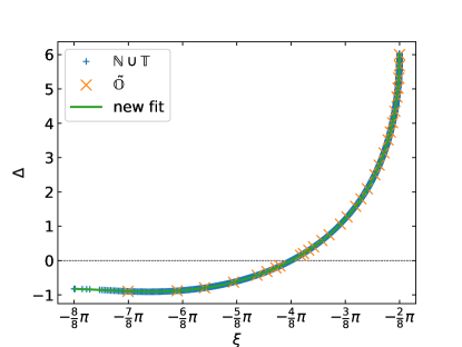
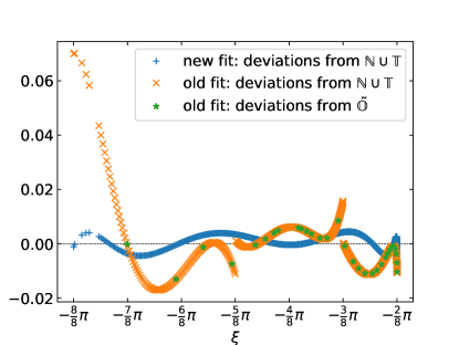
Figure 3: Left panel: comparison of the new parametrization (19) with the new and old data sets. Right panel: deviations of the new parametrization (19) and the old parametrization from the new data set.

In the right panel of Fig. 3, we show the deviations of the two parametrizations from the new data set. Clearly, the new parametrization has a maximum deviation that is about one order of magnitude smaller and is smooth everywhere by construction. A more detailed comparison of the fits can be found in Appendix C. Better accuracy could be achieved by using more coefficients and/or keeping more digits of the coefficients, but the parametrization (19) is a good compromise between accuracy and user friendliness.

IV Range Corrections

On the one hand, Kievsky and Gattobigio have shown that the Efimov radial law, given in Eq. (8), can be generalized to include range corrections by making some minor modifications Kievsky:2012ss :

$$\frac{E_{3}^{(n)}}{E_{2}} = \tan^{2}\xi\,,$$

$$\kappa^{(n)}_{*}a_{B}+\Gamma^{(n)} = \frac{e^{-\Delta\left(\xi\right)/(2s_{0})}}{\cos\xi}\,,$$ (20)

where

$$\frac{1}{a_{B}}=\frac{\sqrt{mE_{2}}}{\hbar}\,$$ (21)

is the binding momentum of the dimer and $\kappa^{(n)}_{*}=\kappa_{*}e^{-n\pi/s_{0}}$. As in the zero-range case, the sign of $a_{B}$ is chosen to be positive if the dimer is bound and negative if the dimer is a virtual state. The radial law now depends on two-parameters: the finite-range parameter $\Gamma^{(n)}$ and the three-body parameter $\kappa^{(n)}_{*}$, both depending on the branch $n$.

Close to the unitary limit, Eq. (20) is well verified by a variety of potentials. The specific value of the finite-range parameter depends very little on the particular form of the potential raquel2016 and can be estimated using a two-parameter potential of Gaussian form. Accordingly, using an S-wave Gaussian interaction of range $r_{0}$, the values of the energy and range parameters for the first three states are given in Table 4.

$n$	0	1	2
$r_{0}\kappa^{(n)}_{*}$	0.4874	0.02124	0.000915
$\Gamma^{(n)}$	0.8472	0.06002	0.0035

Table 4: The three-body parameter $\kappa^{(n)}_{*}$, in units of the Gaussian range $r_{0}$, and the finite-range parameter $\Gamma^{(n)}$ for lowest three states.

On the other hand, Ji et al. Ji:2015hha have shown that the range corrections can approximately be taken into account by introducing a running three-body parameter:

$$\bar{\kappa}_{*}(\mu_{0},a)\equiv(\mu_{0}/\kappa_{*})^{-\gamma r_{s}/a}\kappa_{*}\,,$$ (22)

where $\gamma=0.351..$, $\mu_{0}$ is a momentum scale, and $r_{s}$ the effective range. The running parameter modifies the zero-range parameter $\kappa_{*}$ at each value of $a$ once range corrections are taken into account. Large logarithms in the range corrections can be avoided by expressing observables in terms of $\bar{\kappa}_{*}$. For each level it corresponds to the three-body parameter $\kappa^{(n)}_{*}$ defined above. Moreover close to the unitary limit $a$ and $a_{B}$ $\rightarrow\infty$ and $\bar{\kappa}_{*}\rightarrow\kappa_{*}$. The running three-body parameter can be expanded around this point as

$$\kappa_{*}\approx\bar{\kappa}_{*}\left(1+\frac{\gamma r_{s}}{a_{B}}\ln(\mu_{0}/\bar{\kappa}_{*})\right)\,,$$ (23)

where the use of $a_{B}$ and $\bar{\kappa}_{*}$ in the small term is equivalent at first order.

In Eq. (20) the running parameter is given in terms of $\Gamma^{(n)}$. The equation can be put in the form

$$e^{-n\pi/s_{0}}\kappa_{*}a_{B}=\kappa^{(n)}_{*}a_{B}+\Gamma^{(n)}\,,$$ (24)

where the binding momentum in the zero-range limit is

$$\kappa_{*}a_{B}=e^{n\pi/s_{0}}\frac{e^{-\Delta\left(\xi\right)/(2s_{0})}}{\cos\xi}\,,$$ (25)

Considering that Eq. (22) implicitely carries a factor $e^{n\pi/s_{0}}$, we can make the following identification

$$\Gamma^{(n)}=\gamma r_{s}\frac{\bar{\kappa}_{*}}{e^{n\pi/s_{0}}}\ln{\left(\frac{\mu_{0}}{\bar{\kappa}_{*}}e^{n\pi/s_{0}}\right)}=\gamma r_{s}\frac{\bar{\kappa}_{*}}{e^{n\pi/s_{0}}}\left(\ln{\left(\frac{\mu_{0}}{\bar{\kappa}_{*}}\right)}+n\pi/s_{0}\right)\,.$$ (26)

This equation shows the functional dependence of the shift $\Gamma^{(n)}$ in terms of the level $n$ and the momentum scale $\mu_{0}$. For a Gaussian of range $r_{0}$ it can be put into the form

$$\Gamma^{(n)}=\gamma(r_{s}/r_{0})\frac{\bar{\kappa}_{*}r_{0}}{e^{n\pi/s_{0}}}\left(\ln{\left(\frac{\mu_{0}}{\bar{\kappa}_{*}}\right)}+n\pi/s_{0}\right)\approx\frac{0.2456}{e^{n\pi/s_{0}}}\left(3.445+n\pi/s_{0}\right)\,,$$ (27)

where we have used the ratio $r_{s}/r_{0}=1.43522$ raquel2016 and the values of $r_{0}\kappa_{*}^{(n)}$ and $\Gamma^{(n)}$ for $n=0$ given in Table 4 to determine $\mu_{0}r_{0}\approx 15.36$. Using these values, we can predict $\Gamma^{(1)}$ and $\Gamma^{(2)}$ from Eq. (27). The corresponding evolution of $\Gamma^{(n)}$ with $n$ is shown in Fig. 4.

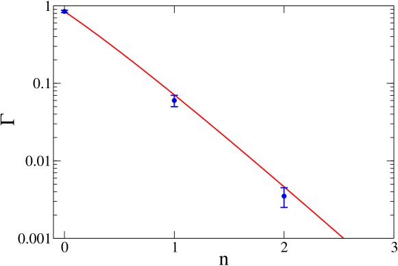
Figure 4: The finite-range parameter $\Gamma^{(n)}$ as a function of the level $n$. The solid line is given by Eq. (26) with $\mu_{0}r_{0}\approx 15.3$ whereas the circles are the values of Table 4. The error bars indicate the spread of different model potentials.

Overall, we find good agreement with the values of $\Gamma^{(1)}$ and $\Gamma^{(2)}$ in Table 4 within the error bars given by the spread of different model potentials. Finally, note that Eq. (27) predicts a correction to the naive expectation $\ln\Gamma^{(n)}=\mbox{const.}-n\pi/s_{0}$ which is confirmed by the finite range results from Gaussian potentials.

V Summary

We have provided a new parametrization of the universal function $\Delta(\xi)$ that appears in Efimov’s equation (7, 8) for the binding energies $E_{3}^{(n)}$ of Efimov states. This equation provides a simple alternative to the solution of the STM integral equations for the calculation of universal Efimov binding energies.

In Ref. Braaten:2002sr , this equation was generalized to include the effects of deep two-body bound states. The generalization involves an additional inelasticity parameter $\eta$, but the spectrum is determined by the same universal function $\Delta(\xi)$ determined here.

A simple modification of Efimov’s universal equation, given in Eq. (20), that can account for effective range corrections was proposed in Ref. Kievsky:2012ss . It was shown to work well for ⁴He atoms and other systems close to the unitary limit. We have quantitatively investigated the connection of this equation to the running three-body parameter introduced by Ji et al. Ji:2015hha in a rigorous perturbative treatment of effective range effects and found good agreement. This result provides further evidence for the validity of the finite range extension of Efimov’s universal equation proposed in Ref. Kievsky:2012ss .

Appendix A Details of the Fitting Methodology

Since plots of the new data set $\mathbb{N}$ together with the values at the thresholds $\mathbb{T}$  questioned the consistency of the resulting data set $\mathbb{N}\cup\mathbb{T}$, we modified the first step of the fitting procedure to address this question. The single Lawson fit is replaced by a series of Lawson fits in the following way: First a set of problematic data points from $\mathbb{N}$ is defined (typically some points around the thresholds from $\mathbb{T}$). Then a Lawson fit without these problematic points is carried out and the deviations of these data points from the resulting function are calculated. Those data points whose deviation is smaller than a given threshold get included and a new fit is done. This procedure is repeated until all points are included or no more points meet the condition.

We used as threshold $1.1d_{\mathrm{max},0}$, where ${d_{\mathrm{max},0}}$ is the maximum absolute deviation of the initial fit. This algorithm had to be employed for all fits with a different number of coefficients. The result of this procedure is that all fits are based on the complete data set $\mathbb{N}\cup\mathbb{T}$ consisting of 5031 data points.

Appendix B Optimized Rounding Procedure

The optimized rounding improves the quality of the parametrization over standard rounding of the fit coefficients, especially when the coefficients are rounded to a low number of decimal digits. Our procedure was as follows: all coefficients $c_{i}$, which are rounded to $n_{i}$ digits, were varied independently within a certain range with a step size of $10^{-n_{i}}$ in order to minimize $d_{\rm max}$, which usually increases by rounding. This procedure was carried out for fits from $6$ up to $11$ coefficients, which were rounded to two and three digits except for the zeroth coefficient. It was rounded to higher number of digits (three or four), since $c_{0}=\Delta\left(-\pi/4\right)$ holds in case of our parametrization. As a consequence we ended up with four different rounding schemes: f3d2, f4d2, f3d3 and f4d3. Here the notation f$x$d$y$ is used with $x$ as the number of decimal digits of the zeroth coefficient $c_{0}$ and $y$ as number of decimal digits of the other coefficients $c_{i>0}$. Thus in total $2\cdot 2\cdot 6=24$ optimized rounding procedures had to be carried out. The interval in which the coefficients were varied in each optimized rounding process was chosen so that in each process effectively about $10^{12}$ variations were tested. This corresponds to 100 variations per coefficient in a fit with 6 coefficients and 13 variations per coefficient in a fit with 11 coefficients.

   

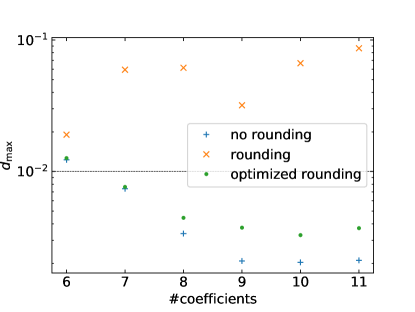
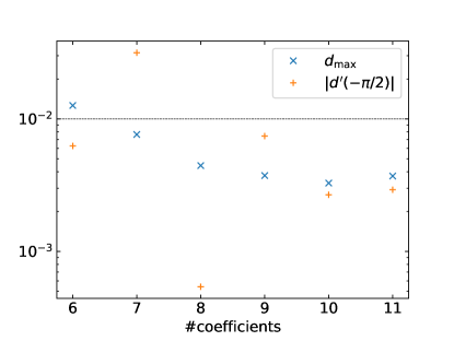
Figure 5: Left panel: maximum absolute deviations $d_{\rm max}$ of the f3d2 fits as function of the number of coefficients. Right Panel: $d_{\rm max}$ and the deviation of the derivative at unitarity $|d^{\prime}\left(-\pi/2\right)|$  after optimized rounding in the f3d2 scheme.

In Fig. 5, we show the deviations of the different fits. These plots clearly show that the optimized rounding leads to a significant reduction of the deviations. We find that rounding the $c_{i>0}$ to two decimal places is enough to have an maximum absolute deviation smaller than $10^{-2}$. In this case at least seven coefficients are necessary. In comparison with the fit with seven coefficients the fit with eight ones has a lower $d_{\rm max}$ and a deviation at $-\pi/4$, which is smaller by more than one order of magnitude. Thus the fit with eight coefficients was chosen. Another advantage of this fit is a much lower deviation of its derivative from $\Delta^{\prime}\left(-\pi/2\right)$, which is approximately given to $2.125850069373$ in Castin:2011 . These observations hold for the rounding schemes f3d2 and f4d2. We selected f3d2, as the absolute deviation at $-\pi/4$ of f4d2 is also greater than $10^{-4}$ and this implies giving $c_{0}$ with four decimal digits is not justifiable. It should be a good compromise between accuracy and usability. It is comparable to the complexity of the old parametrization (10).

Appendix C Comparison of Different Parametrizations

In Table 5 the new parametrization is compared to the parametrization from Braaten:2002sr (respectively Braaten:2004rn ) and the one given in Naidon:2016dpf .

Table 5: Comparison of fits. One should note that we do not know which data set was used for the creation of the parametrization from Naidon:2016dpf . $d_{\rm max}$ is computed using $\mathbb{N}\cup\mathbb{T}$, $d\left(\xi\right)$ denotes the deviation from $\mathbb{N}\cup\mathbb{T}$ at $\xi$. $d^{\prime}\left(\xi\right)$ denotes the deviation of the derivative at $\xi$.

Fit	$d_{\rm max}$	$|d\left(-\pi\right)|$	$|d\left(-\pi/2\right)|$	$|d\left(-\pi/4\right)|$	$|d^{\prime}\left(-\pi/2\right)|$
Old fit	7.01 $\cdot 10^{-2}$	6.99 $\cdot 10^{-2}$	6.15 $\cdot 10^{-3}$	6.55 $\cdot 10^{-3}$	5.85 $\cdot 10^{-3}$
Fit from Naidon:2016dpf	8.64 $\cdot 10^{-3}$	1.20 $\cdot 10^{-3}$	0.00 $\cdot 10^{0}$	3.07 $\cdot 10^{-4}$	1.59 $\cdot 10^{-2}$
New fit	4.44 $\cdot 10^{-3}$	1.07 $\cdot 10^{-3}$	3.78 $\cdot 10^{-4}$	3.07 $\cdot 10^{-4}$	5.42 $\cdot 10^{-4}$

References

- (1) E. Braaten and H.-W. Hammer, Phys. Rept. 428, 259 (2006).
- (2) V. N. Efimov, Sov. J. Nucl. Phys. 12, 589 (1971); 29, 546 (1979); Nucl. Phys. A 210, 157 (1973).
- (3) P. F. Bedaque, H.-W. Hammer, and U. van Kolck, Phys. Rev. Lett. 82, 463 (1999); Nucl. Phys. A 646, 444 (1999).
- (4) B. D. Esry, C. H. Greene, and J. P. Burke, Phys. Rev. Lett. 83, 1751 (1999).
- (5) E. Braaten and H.-W. Hammer, Phys. Rev. Lett. 87, 160407 (2001).
- (6) R. E. Grisenti, W. Schöllkopf, J. P. Toennies, G. C. Hegerfeldt, T. Köhler and M. Stoll, Phys. Rev. Lett. 85, 2284 (2000).
- (7) W. Schöllkopf and J.W. Toennies, Science 266, 1345 (1994).
- (8) M. Kunitski, S. Zeller, J. Voigtsberger, A. Kalinin, L. Ph. H. Schmidt, M. Schöffler, A. Czasch, W. Schöllkopf, R. E. Grisenti, T. Jahnke, D. Blume, and R. Dörner, Science 348, 551 (2015).
- (9) C. Chin, R. Grimm, P. Julienne, and E. Tiesinga, Rev. Mod. Phys. 82, 1225 (2010).
- (10) E. Braaten and H.-W. Hammer, Ann. Phys. 322, 120 (2007).
- (11) P. Naidon and S. Endo, Rept. Prog. Phys. 80, 056001 (2017).
- (12) E. Braaten, H.-W. Hammer and M. Kusunoki, Phys. Rev. A 67, 022505 (2003).
- (13) D. V. Fedorov and A. S. Jensen, Phys. Rev. Lett. 71, 4103 (1993);
- (14) E. Nielsen, D. V. Fedorov, A. S. Jensen, E. Garrido, Phys. Rep. 347, 373 (2001).
- (15) A. Kievsky and M. Gattobigio, Phys. Rev. A 87, 052719 (2013).
- (16) G. V. Skorniakov and K. A. Ter-Martirosian, Sov. Phys. JETP 4, 648 (1957) [J. Exptl. Theoret. Phys. (U.S.S.R.) 31, 775 (1956)].
- (17) V. F. Kharchenko, Sov. J. Nucl. Phys. 16, 173 (1973) [Yad. Fiz. 16, 310 (1972)].
- (18) H.-W. Hammer and T. Mehen, Nucl. Phys. A 690, 535 (2001).
- (19) A. O. Gogolin, C. Mora and R. Egger, Phys. Rev. Lett. 100, 140404 (2008).
- (20) C. L. Lawson, Ph.D. thesis, UCLA, 1961.
- (21) J. R. Rice and K. H. Usow, Math. Comp. 22, 118 (1968).
- (22) R. Álavrez-Rodríguez, A. Deltuva, M. Gattobigio and A. Kievsky, Phys. Rev. A 93, 062701 (2016).
- (23) C. Ji, E. Braaten, D. R. Phillips and L. Platter, Phys. Rev. A 92, 030702 (2015).
- (24) Y. Castin and F. Werner, Phys. Rev. A 83, 063614 (2011).