Analog quantum simulation of the spinor-4 Dirac equation with an artificial gauge field

Abstract

A two-dimensional spatially and temporally modulated Wannier-Stark system of ultracold atoms in optical lattices is shown to mimic the behavior of a Dirac particle. Suitable additional modulations generate an artificial gauge field which simulates a magnetic field and imposes the use of the full spinor-4 Dirac equation.

I Introduction

The Dirac equation, unifying quantum mechanics and special relativity, is a major achievement in physics. It has vast implications in several fields, e.g. particle physics where it describes spin-1/2 leptons and their interactions with photons, condensed matter where it is used as a model for several types of quasiparticles, and also in the fast progressing field of topological insulators.

Although the Dirac equation represents a paradigm for modern field theory, this physics remained relatively elusive, restricted to high-energy situations or to exotic materials. Recent developments both in condensed matter and ultracold-atom systems have generated a burst of interest, in particular, the concept of “quantum simulator” opened a new window in the study of Dirac physics (Park et al., 2019; Garreau and Zehnlé, 2017; Lopez-Gonzalez et al., 2014; Qu et al., 2013; Tarruell et al., 2012; Mazza et al., 2012; Zhang et al., 2012; Gerritsma et al., 2011; Lamata et al., 2011; Gerritsma et al., 2010; Longhi, 2010; Dreisow et al., 2010; Witthaut et al., 2011). Inspired by an original insight of Feynman (Feynman, 1982), an analog quantum simulator (as opposed to quantum-computer simulations) is a “simple” and controllable system that can mimic (some aspects of) the behavior of a more complex or less accessible ones. The flexibility of ultracold-atom systems also prompted for innovative ideas like the generation of the so-called “artificial” gauge fields acting on (neutral) atoms that mimic the effects of an electromagnetic field (Dalibard et al., 2011), allowing for the study of quantum magnetism (Aidelsburger et al., 2013), engineered spin-orbit coupling, and topological systems (Galitski and Spielman, 2013). The mixing of these ideas with the physics of ultracold atoms in optical lattices has proven extremely fruitful (Bloch et al., 2008; Dalibard et al., 2011; Bloch et al., 2014; Georgescu et al., 2014; Goldman et al., 2016; Gross and Bloch, 2017; Garreau, 2017).

The Dirac equation is the most complete formulation describing a relativistic charged fermion of spin 1/2. It leads to a spinor-4 description which automatically includes the spin and the electron antiparticle, the positron. In the rest frame of the free particle, which always exists for a massive particle, the spinor-4 components can be separated in two spinor-2 obeying equivalent equations. In the presence of electromagnetic fields, however, the two spinor-2 for a massive particle generally obey different equations, and a full spinor-4 description is necessary. The aim of the present work is the elaboration of a minimal model analog to a 2D Dirac equation in the presence of an artificial gauge field (related to a vector potential $\boldsymbol{A}$ with non-zero rotational). In this case the spinor-4 description is mandatory, and we show that the main characteristics of a Dirac particle are obtained.

In a previous work (Garreau and Zehnlé, 2017) we introduced a general model allowing to mimicking a spinor-4 Dirac Hamiltonian in 1D without magnetic field. In the present work we combine time- and space-tailored optical potentials acting on independent atoms in order to obtain a 2D Dirac Hamiltonian of the form

$$H_{D}=c\boldsymbol{\alpha}\cdot\left(\boldsymbol{p}-q\boldsymbol{A}\right)+\beta m_{D}c^{2}$$ (1)

where $c$ is the velocity of light, $m_{D}$ and $q$ are the Dirac particle’s mass and charge, $\boldsymbol{p}$ is the momentum and $\boldsymbol{A}$ the vector potential. The $4\times 4$ Dirac matrices constructed from Pauli matrices $\sigma_{i}$ ($i=x,y,z$) are:

$$\alpha_{i}=\left(\begin{array}[]{cc}0&\sigma_{i}\\ \sigma_{i}&0\end{array}\right)\qquad\beta=\left(\begin{array}[]{cc}\boldsymbol{1}&0\\ 0&-\boldsymbol{1}\end{array}\right).$$

and $\boldsymbol{1}$ is the $2\times 2$ unit matrix. With this we i) generalize this approach to the 2D case, ii) introduce an artificial gauge field, and iii) demonstrate its ability to simulate known properties of the Dirac equation. To the best of our knowledge, such a complete Dirac simulator has not been proposed in the literature, and opens new ways for a deeper exploration of the Dirac physics.

II Spinor-4 Dirac quantum simulator in 2D

We first construct a modulated 2D tilted optical lattice model that mimics a 2D spinor-4 Dirac equation with no field. The model builds on the general approach introduced for the 1D case in Ref. (Garreau and Zehnlé, 2017). A 2D “tilted” (or Wannier-Stark) lattice in the $x,z$ plane  is described by the 2D (dimensionless) Hamiltonian

$$H_{0}=\frac{p_{x}^{2}+p_{z}^{2}}{2m^{*}}+V_{L}(x,z)+F_{x}x+F_{z}z$$ (2)

with $\boldsymbol{p}=p_{x}\mathbf{x}+p_{z}\mathbf{z}$ the momentum in 2D ($\mathbf{x},\mathbf{z}$ are unit vectors in the directions $x,z$), $\boldsymbol{F}=F_{x}\mathbf{x}+F_{z}\mathbf{z}$ a constant force and $V_{L}$ a square lattice formed by orthogonal standing waves

$$V_{L}(x,z)=-V_{1}\left[\cos(2\pi x)+\cos(2\pi z)\right]$$

where space is measured in units of the step $\mathsf{a}$  of the square lattice $V_{L}$, $\mathsf{a}=\lambda_{L}/2$ if the lattice is formed by counter-propagating beams of wavelength $\lambda_{L}=2\pi/\mathrm{k}_{L}$. Time is measured in units of $\hbar/\mathsf{E}_{R}$ where $\mathsf{E}_{R}=\hbar^{2}\mathrm{k}_{L}^{2}/2\mathrm{M}$ is the atom’s recoil energy ($\mathrm{M}$ is the atom’s mass). With these choices, $m^{*}=\pi^{2}/2$ , $\hbar=1$ and $p_{j}=-i\partial_{j}$ ($j=x,z)$. Since the Hamiltonian Eq. (2) is separable, its eigenstates can be factorized in terms of localized Wannier-Stark (WS) functions $\varphi_{n}^{(x,y)}$ (Wannier, 1960; Zener, 1934) which are exact eigenstates of a tilted one-dimensional lattice (Garreau and Zehnlé, 2017):

$$\Phi_{n,m}(x,z)=\varphi_{n}^{(x)}(x)\varphi_{m}^{(z)}(z)$$

where the integer index $n$ indicates the lattice site along the $x$ direction where the eigenfunction $\varphi_{n}^{(x)}(x)$ is centered (resp. $m$ in the $z$ direction). The energies of the system are then

$$E_{n,m}=E_{0}+n\omega_{B}^{(x)}+m\omega_{B}^{(z)}$$ (3)

where $E_{0}$ is an energy offset with respect to the bottom of the central well $n=m=0$. The energy spacing in directions $x$ and $z$ define the so-called Bloch frequencies, $\omega_{B}^{(x)}=F_{x}$ ($=\mathsf{F}_{x}\mathsf{a}/\hbar$ in dimensionfull units) and $\omega_{B}^{(z)}=F_{z}$, where we intentionally choose $F_{z}\neq F_{x}$. This defines the lowest “Wannier-Stark ladder” of energy levels separated by integer multiples of $\omega_{B}^{(x,z)}$, Eq. (3). According to the potential parameters, there can be “excited” ladders, also obeying Eq. (3), but with higher values of $E_{0}$. As in Ref. (Garreau and Zehnlé, 2017), we assume here that the excited ladders are never populated and that the dynamics occurs only among the lowest-ladder WS states of each site.

   

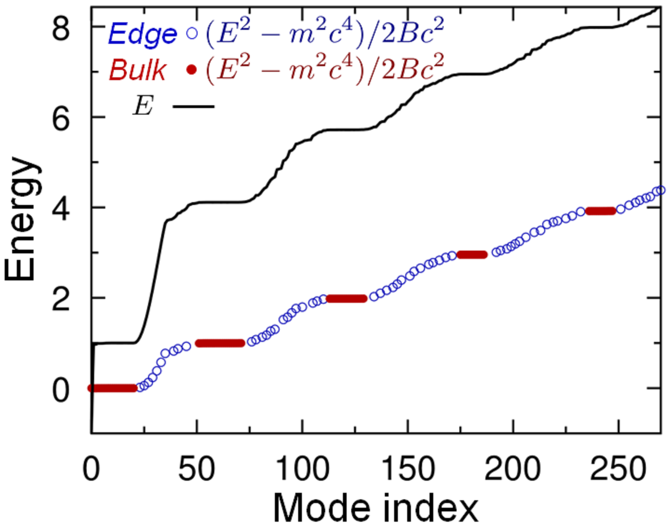
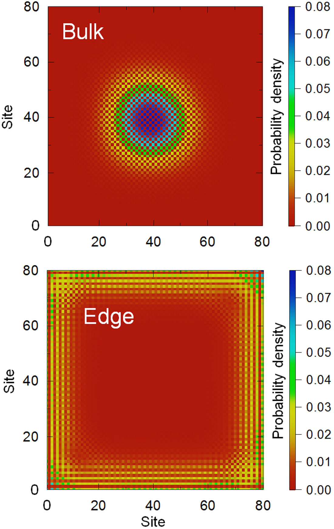
Figure 1: Left: Eigenvalue spectrum of the quantum simulator. The black solid line displays the positive raw energies $E$ as a function of an arbitrary mode index (negative energies $E\rightarrow-E$ are not displayed for clarity). The blue circles and red disks display the quantity $\widetilde{E}=\left(E^{2}-m^{2}c^{4}\right)/2Bc^{2}$, Eq. (18). The red plateaus correspond to bulk states which, according Eq. (19), are very close to integers. The blue parts correspond to “edge” states which are due to the finite size of the simulated lattice. Right: Examples of a bulk state (top) corresponding to an integer value of $\widetilde{E}$ and of an edge state (bottom) corresponding to an intermediate, non-integer value. The simulation parameters are $mc^{2}=1$, $c_{S}=20$ and $B=1/50$, and the model parameters in Eq. (12) are $T_{0}=1$, $T_{x}=T_{y}=-10i$ , and $T_{x}^{A}=-T_{z}^{A}=1/10$.

The Hamiltonian Eq. (2) is invariant under a translation by an integer multiple $n$ of the lattice step $a=1$ (in dimensionless units) in the $x$ direction provided that the energy is also shifted by $nF_{x}$ (resp. $mF_{z}$ in the $z$ direction), hence the eigenstates are such that

$$\varphi_{n}^{(x)}(x)=\varphi_{0}^{(x)}(x-n),$$ (4)

(resp. $\varphi_{m}^{(z)}(z)=\varphi_{0}^{(z)}(z-m)$ in the $z$ direction).

Our aim is to obtain an effective evolution equation for the system equivalent to a 2D Dirac equation Eq. (1) for a particle of mass $m$

$$i\partial_{t}\left[\Psi\right]=\left\{c\alpha_{x}\left(p_{x}-A_{x}\right)+c\alpha_{z}\left(p_{z}-A_{z}\right)+\beta mc^{2}\right\}\left[\Psi\right]$$ (5)

where $\partial_{t}\equiv\partial/\partial t$, $\left[\Psi\right]$ denotes a spinor-4, and $\boldsymbol{A}=A_{x}\mathbf{x}+A_{z}\mathbf{z}$. The effective speed of light is $c=\hbar\mathrm{c}/\mathsf{a}\mathsf{E}_{R}$, the gauge field $\boldsymbol{A}=q\mathsf{a}\mathbf{A}/\hbar$, the mass $m=\mathsf{E}_{R}\mathsf{a}^{2}m_{D}/\hbar^{2}$, and effective charge is set to unity.

Consider first the case without gauge field ($\boldsymbol{A}=0$). We can induce controlled dynamics (Garreau and Zehnlé, 2017) in the system by adding to $H_{0}$, Eq. (2), a resonant time-dependent perturbation of the form

$$\bar{V}(x,z,t)= V_{x}\cos\left(2\pi x\right)\sin(\omega_{B}^{(x)}t)+$$

$$V_{z}\cos\left(\pi x\right)\cos\left(2\pi z\right)\sin(\omega_{B}^{(z)}t).$$ (6)

The utility of the term proportional to $\cos(\pi x)$ with spatial periodicity $2$ will appear below.

The general solution of the corresponding Schrödinger equation can be decomposed on the eigenbasis $\Phi_{n,m}(x,z)$ :

$$\psi(x,z,t) =\sum_{n,m}c_{n,m}(t)\exp\left[-i\left(n\omega_{B}^{(x)}+m\omega_{B}^{(z)}\right)t\right]$$

$$\times\varphi_{n}^{(x)}(x)\varphi_{m}^{(z)}(z)$$

where $c_{n,m}$ are complex amplitudes. Taking into account the Hamiltonian $H_{0}+\bar{V}$, one obtains the following set of coupled differential equations for the amplitudes

$$id_{t}c_{n,m}=\sum_{j,k\in\mathbb{Z}} \left\{\left\langle n,m\right|\bar{V}\left|n+j,m+k\right\rangle\right.$$

$$\left.\times\exp\left[-i\left(j\omega_{B}^{(x)}+k\omega_{B}^{(z)}\right)t\right]c_{n+j,m+k}\right\}$$ (7)

where $d_{t}\equiv d/dt$ and we simplified the notation $\left|\varphi_{n}^{(x)}\right\rangle\otimes\left|\varphi_{m}^{(z)}\right\rangle\equiv\left|n,m\right\rangle$. To the dominant order, one can neglect non-resonant terms and keep nearest neighbor couplings only, i.e take only $j=\pm 1$ and $k=\pm 1$ in Eq. (7) (see Appendix A).  The time modulation at the Bloch frequencies $\omega_{B}^{(x)}$ (resp. $\omega_{B}^{(z)}$) resonantly couples first-neighbor WS states in the $x$ direction (resp. $z$ direction). Note that as we assume $\omega_{B}^{(x)}\neq\omega_{B}^{(z)}$ resonant couplings in both direction $x$ and $z$ can be controlled independently.

Taking into account the choice of perturbation $\bar{V}$ of Eq. (6), the couplings in Eq. (7) are proportional to the spatial overlap amplitudes

$$\left\langle\varphi_{n}^{(x)}\right|\cos\left(2\pi x\right)\left|\varphi_{n\pm 1}^{(x)}\right\rangle=\left\langle\varphi_{0}^{(x)}\right|\cos\left(2\pi x\right)\left|\varphi_{1}^{(x)}\right\rangle\equiv\Omega_{x}$$

[see. Eq. (4)] in the $x$ direction, and

$$\left\langle\varphi_{n}^{(x)}\right|\cos\left(\pi x\right)\left|\varphi_{n}^{(x)}\right\rangle\left\langle\varphi_{m}^{(z)}\right|\cos\left(2\pi z\right)\left|\varphi_{m\pm 1}^{(z)}\right\rangle$$

$$=\left(-1\right)^{n}\left\langle\varphi_{0}^{(x)}\right|\cos\left(\pi x\right)\left|\varphi_{0}^{(x)}\right\rangle\left\langle\varphi_{0}^{(z)}\right|\cos\left(2\pi z\right)\left|\varphi_{1}^{(z)}\right\rangle$$

$$=\left(-1\right)^{n}\Omega_{z}$$

in the $z$ direction. The $(-1)^{n}$ contribution comes from the spatial modulation in $\cos(\pi x)$ in Eq. (6) which has a period of two lattice steps [see Eq. (23) in Appendix A] and introduces a distinction between even and odd sites in the $x$ direction.

From Eq. (7), one obtains a set of differential equations with nearest-neighbor couplings.

$$id_{t}c_{n,m}= T_{x}\left(c_{n+1,m}-c_{n-1,m}\right)$$

$$+(-1)^{n}T_{z}\left(c_{n,m+1}-c_{n,m-1}\right)$$ (8)

where $T_{x}=-iV_{x}\Omega_{x}/2$ and $T_{z}=-iV_{z}\Omega_{z}/2$.

Assuming that the wave packet is large and smooth at the scale of the lattice step one can take the continuous limit of Eq. (8), and associate the discrete amplitudes $c_{n,m}(t)$ to two continuous functions. Since the site parity dependence in Eq. (8) must be taken into account, we introduce the functions $s_{ee}(x,z,t)$ which is the envelope of $c_{n,m}$ for $n,m$ even, $s_{eo}(x,z,t)$ which is the envelope of $c_{n,m}$ for $n$ even and $m$ odd, and analogously for $s_{oe}$ and $s_{oo}$. These functions can be arranged as components of a spinor-4 $[\Psi]=\left(s_{ee},s_{oo},s_{eo},s_{oe}\right){}^{\intercal}$ describing 4 coupled sub-lattices, which, from Eq. (8), obey a Hamiltonian equation

$$id_{t}\left[\Psi(x,z,t)\right]=H_{S}\left[\Psi(x,z,t)\right]$$ (9)

where $H_{S}$ can be easily shown to be analogous to a 2D Dirac Hamiltonian of the form $H_{S}=c_{S}\mathbf{\boldsymbol{\alpha}}\cdot\boldsymbol{p}$ with an effective velocity of light $c_{S}=V_{x}\Omega_{x}=V_{z}\Omega_{z}$ (these terms can be made equal by adequately tuning the modulation amplitudes $V_{x,z}$, but one can also create an anisotropic model with $c_{S_{x}}\neq c_{S_{z}}$, with the possibility of an effective violation of Lorentz invariance (Park et al., 2019)). The above system can be broken into two equivalent set of equations (Garreau and Zehnlé, 2017) which correspond to the well-known massless Weyl spinor-2 fermion. The twofold-degenerated dispersion relation deduced from Eq. (9) is $\omega(k)=\pm\left(\Omega_{x}^{2}k_{x}^{2}+\Omega_{z}^{2}k_{z}^{2}\right)^{1/2}$ and corresponds, as it could be expected, to a Dirac cone.

The Hamiltonian of a massive particle can be generated by adding a static perturbation $V_{0}\cos(\pi x)\cos(\pi z)$ to Eq. (6). Then, neglecting derivatives $\partial_{x,z}^{2}c_{m,n}$ or higher, Eq. (8) takes the form

$$id_{t}c_{n,m}= (-1)^{n+m}T_{0}+(-1)^{n}T_{z}\left(c_{n,m+1}-c_{n,m-1}\right)$$

$$+T_{x}\left(c_{n+1,m}-c_{n-1,m}\right)$$ (10)

where $T_{0}=V_{0}\left\langle\varphi_{0}^{(z)}\right|\cos(\pi z)\left|\varphi_{0}^{(z)}\right\rangle\left\langle\varphi_{0}^{(x)}\right|\cos(\pi x)\left|\varphi_{0}^{(x)}\right\rangle$. In the continuous limit one obtains a 2D Dirac Hamiltonian for a finite-mass particle $H_{S}=c_{S}\mathbf{\boldsymbol{\alpha}\cdot p}+\beta mc^{2}$ with an effective rest energy $mc^{2}=T_{0}$. This term opens a gap of width $2mc^{2}$ in the the dispersion relation, separating “particle” and “antiparticle” states, exactly as in the Dirac equation.

The approximations used in construction of the above model are well understood and controlled. As the system is to a very good approximation a closed one (even experimentally), there is only a small broadening of the resonances, which make these resonances highly selective. Next-to-neighbor couplings are out of resonance and are thus negligible, and the same is true for intrawell couplings between different ladders. For particular values of the potential parameters $(V_{x,z},F_{x,z})$ “accidental” resonances can occur, but these exotic situations are not considered here. The accuracy of our approach can also be checked by comparing the results of the model to a simulation of the full Schrödinger equation, which takes into account all existing couplings, as we have done with the simpler, but conceptually equivalent, 1D model in Ref. (Garreau and Zehnlé, 2017). For the very same reason (the sharpness of the resonances) the system is not expected to be particularly sensitive to heating caused by experimental noise.

III Dirac equation with an artificial gauge field

In this section, we show how the analogous of a “non-trivial” (i.e. of non-zero rotational) vector potential $\boldsymbol{A}=A_{x}\mathbf{x}+A_{z}\mathbf{z}$ with $A_{x}\propto z$ and $A_{z}\propto x$, can introduced in the system. The Dirac Hamiltonian of Eq. (1) can be realized by adding to Eq. (6) an additional perturbation

$$\bar{V}_{A}(x,z,t)= V_{x}^{A}z\cos\left(2\pi x\right)\cos(\omega_{B}^{(x)}t)+$$

$$V_{z}^{A}x\cos\left(\pi x\right)\cos\left(2\pi z\right)\cos(\omega_{B}^{(z)}t).$$ (11)

This term can be treated in the same way as in Sec. II and leads to

$$id_{t}c_{n,m} =(-1)^{n+m}T_{0}+(-1)^{n}T_{z}\left(c_{n,m+1}-c_{n,m-1}\right)$$

$$+T_{x}\left(c_{n+1,m}-c_{n-1,m}\right)$$

$$+T_{x}^{A}m\left(c_{n+1,m}+c_{n-1,m}\right)$$

$$+(-1)^{n}nT_{z}^{A}\left(c_{n,m+1}+c_{n,m-1}\right)$$ (12)

where $T_{z}^{A}=\frac{1}{2}\Omega_{z}V_{z}^{A}$, $T_{x}^{A}=\frac{1}{2}\Omega_{x}V_{x}^{A}$. The additional terms on the last two lines in Eq. (12) are due to the potential Eq. (11) which generates the slopes proportional to $m$ (resp. $n$) in direction $z$ (resp. $x$) .

In the continuous limit, and neglecting second order and higher derivatives of the spinor components, we obtain the Hamiltonian Eq. (1), with an artificial gauge field $\boldsymbol{A}=-2(zT_{x}^{A}\mathbf{x}+xT_{z}^{A}\mathbf{z})/c_{S}$ (cf. App. A). The symmetric gauge considered in the next section can be realized by tuning the modulation amplitudes in $\bar{V}_{A}$ so that $T_{x}^{A}=-T_{z}^{A}$, so that $\boldsymbol{A}=2T_{z}^{A}(z\mathbf{x}-x\mathbf{z})/c_{S}$, corresponding to a uniform magnetic field in the $y$ direction $\boldsymbol{B}=4T_{z}^{A}\mathbf{y}/c_{S}$ .

 

 

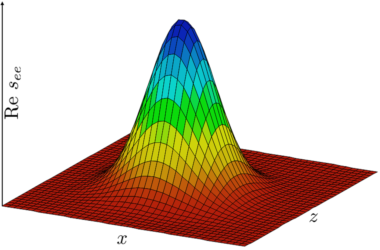
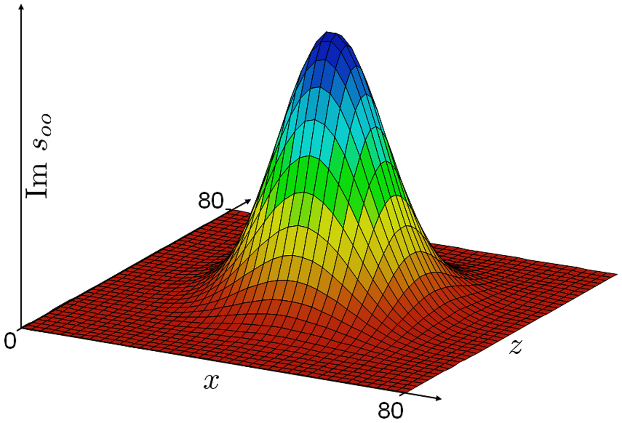
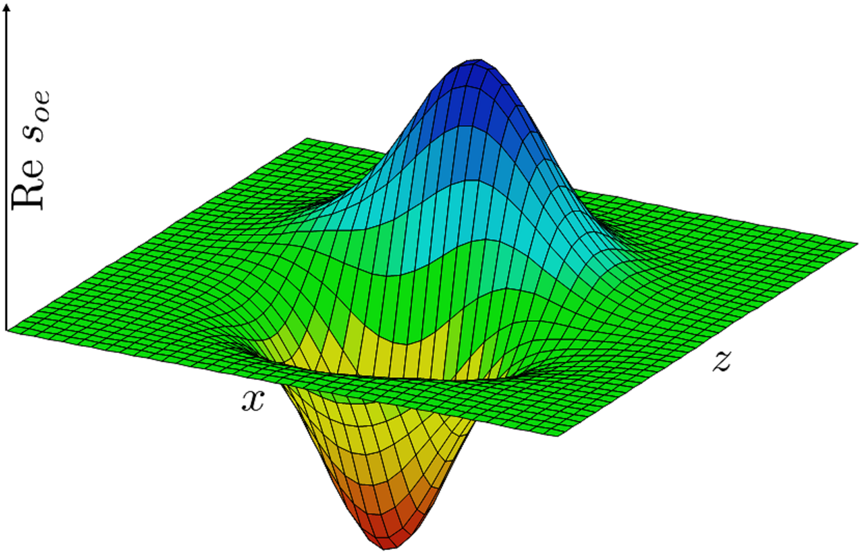
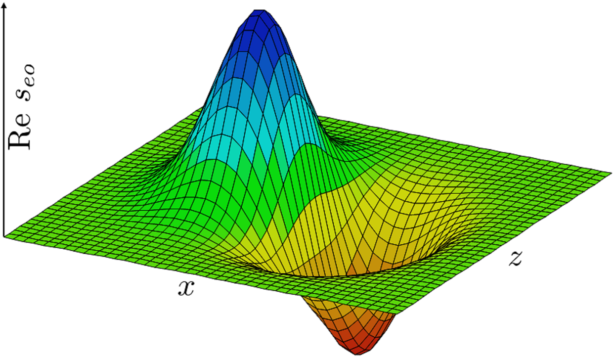
Figure 2: First “bulk” excited eigenstate of Eq. (20). Four components of the spinor are shown: Re($s_{ee}$), Im($s_{oo}$), Re($s_{oe}$), Re($s_{eo}$). The first excited energy is $E=4.11$ (same parameters as in Fig.  1). The WS numerical simulation was performed in a square of $80\times 80$ lattice sites (shown in only one plot, for clarity).

IV Quantum simulation of Dirac physics

We briefly recall well-known theoretical results of Eq. (5) for a spinor-4 Dirac particle in the presence of a symmetric vector potential $\boldsymbol{A}=2T_{z}^{A}(z\mathbf{x}-x\mathbf{z})/c_{S}$. We will compare them with the numerical results of the discrete model Eq. (12) and show that they are in very good agreement, proving that the discrete model reproduces to a good level of accuracy the Dirac physics.

In the following, we write the spinor-4 as $\left[\Psi\right]=\left(\begin{array}[]{c}\phi\\ \chi\end{array}\right)$ where $\phi,\chi$ are spinor-2s. With this convention, the Dirac equation can be decomposed in 2 coupled equations

$$(E-mc^{2})\phi =c\left[\boldsymbol{\sigma}\cdot\left(\boldsymbol{p}-\boldsymbol{A}\right)\right]\chi$$ (13)

$$(E+mc^{2})\chi =c\left[\boldsymbol{\sigma}\cdot\left(\boldsymbol{p}-\boldsymbol{A}\right)\right]\phi.$$ (14)

These equations are symmetric under the transposition $E,$$\phi$, $\chi$ $\longleftrightarrow$ $-E,$$-\chi$, $\phi$ so that the negative energy states are easily deduced from their positive energy counterparts.

Eliminating $\chi$ from Eqs. (14) gives $(E^{2}-m^{2}c^{4})\phi=c\left[\boldsymbol{\sigma}\cdot\left(\boldsymbol{p}-\boldsymbol{A}\right)\right]^{2}\phi$, and, after some straightforward algebra, one finds

$$(E^{2}-m^{2}c^{4})\phi= c^{2}\left[\left(p^{2}+\frac{B^{2}}{4}(x^{2}+z^{2})+L_{y}B\right)\mathbf{1}+\sigma_{y}B\right]\phi$$ (15)

where $L_{y}=(zp_{x}-xp_{z})$ is the angular momentum component in the $y$ direction, with a “diamagnetic” term proportional to $x^{2}+z^{2}$ and “paramagnetic” terms of the type $\boldsymbol{L}\cdot\boldsymbol{B}$ and $\boldsymbol{\sigma}\cdot\boldsymbol{B}$. This equation has “spin up” $\phi_{+}$ and “spin down” $\phi_{-}$ spinor-2  solutions

$$\phi_{\pm}=(1,\pm i)^{\intercal}\psi_{\pm}(x,z)$$ (16)

where the functions $\psi_{\pm}(x,z)$ obey the following equation

$$\left[\frac{p^{2}}{2\mu}+\frac{\mu}{2}(x^{2}+z^{2})+L_{y}\right]\psi_{\pm}=(\widetilde{E}\mp 1)\psi_{\pm}$$ (17)

with

$$\widetilde{E}=(E^{2}-m^{2}c^{4})/(Bc^{2})$$ (18)

and $\mu=B/2$, which strongly evokes a 2D harmonic oscillator of mass $\mu$ and natural frequency $\omega=1$ in a magnetic field.

 
 

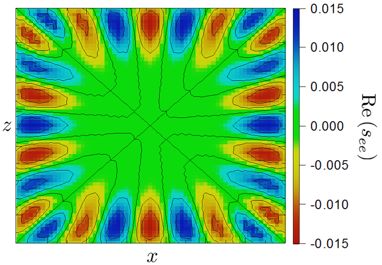
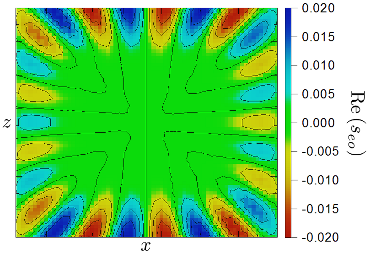
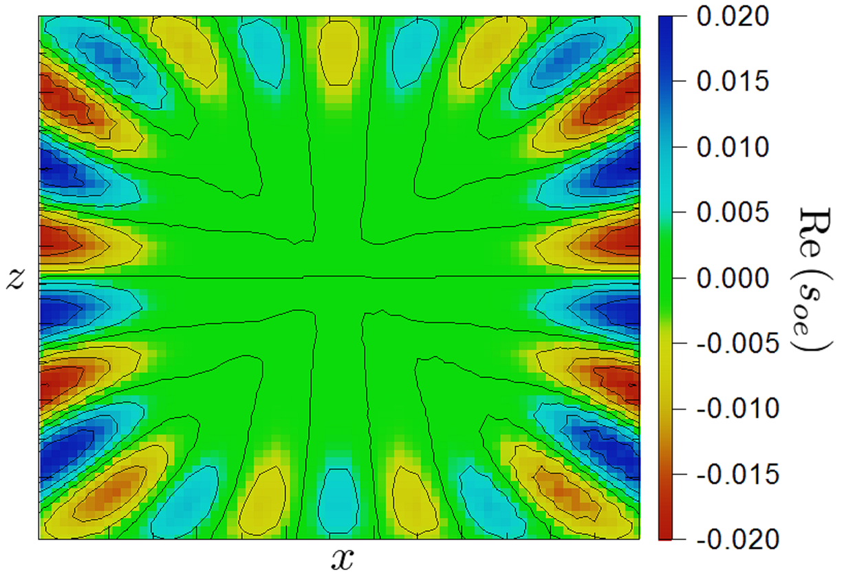
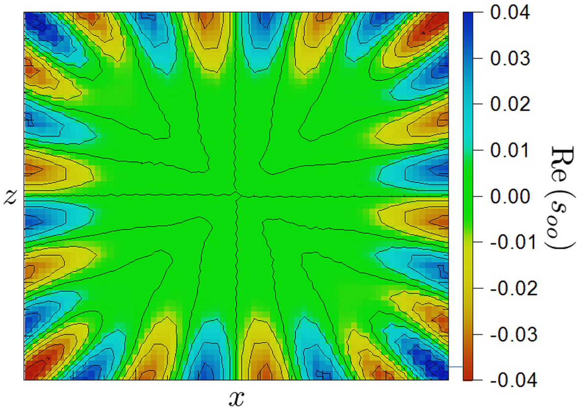
Figure 3: Chiral border state. The real part of the spinor-4 components $s_{ee},s_{eo},s_{oe},s_{oo}$ clearly display a wave propagating along the borders. The imaginary parts are analogous, but dephased of $\pi/2$.

Solutions of Eq. (17) are the well-known “Landau levels”, with spectrum

$$E=\sqrt{m^{2}c^{4}+2Bc^{2}n}$$ (19)

where $n$ (not to be confused with the site index $n$, which does not appear in the present section) is a strictly positive natural number for “spin up” solution $\phi_{+}$ and a natural number for “spin down” $\phi_{-}$. For each $n$ the corresponding energy is infinitely degenerated.

The solutions of Eq. (17) are also well known, and together with Eq. (16) and Eq. (14) lead to solutions for the full eigenspinors $\left[\Psi\right]$. In polar coordinates $x=r\cos\varphi$, $z=r\sin\varphi$ and $\rho=r/\ell$, where $\ell=\sqrt{2/B}$ is an effective dimensionless “magnetic length”, an example of solution for the fundamental level $E=mc^{2}$ is

$$\left(\begin{array}[]{c}\phi\\ \chi\end{array}\right)=\mathscr{N}\left(\begin{array}[]{c}(1,-i)^{\intercal}\exp(-\rho^{2}/2)\\ (0,0)^{\intercal}\end{array}\right)$$

where $\mathscr{N}$ is a normalization factor. There is a corresponding negative energy $E=-mc^{2}$ counterpart with $\phi\rightarrow\phi$ and $\chi\rightarrow-\chi$. Examples of eigenstates belonging to the $n=1$ excited state family $E=\left(m^{2}c^{4}+2Bc^{2}\right)^{1/2}$

$$\left(\begin{array}[]{c}\phi\\ \chi\end{array}\right)=\mathscr{N}\left(\begin{array}[]{c}(1,i)^{\intercal}\\ (1,-i)^{\intercal}\beta\rho\exp(-i\varphi)\end{array}\right)\exp(-\rho^{2}/2)$$ (20)

or

$$\left(\begin{array}[]{c}\phi\\ \chi\end{array}\right)=\mathscr{N}\left(\begin{array}[]{c}(1,-i)^{\intercal}\rho\exp(-i\varphi)\\ (1,i)^{\intercal}\beta\end{array}\right)\exp(-\rho^{2}/2)$$

where $\beta=-2c/\left[\ell(mc^{2}+E)\right]$ .

Numerical simulations of the discrete model reproduce the characteristics of the above solutions of the Dirac equation. According to Eq. (19), plateaus are obtained at integer values $n=\left(E^{2}-m^{2}c^{4}\right)/2Bc^{2}$. As shown in Fig. 1, the numerical solution of Eq. (12) displays such a behavior, with plateaus (red disks) appearing as expected at integer values. The simulation also shows eigenenergies which fall at non-integer values (blue circles); we checked that these are edge states due to finite size effects, as the numerical simulation is performed in a square box containing finite number of lattice sites (80$\times$80) .

Figure 2 shows a numerical example of the the four components of the eigenspinor $\left[\Psi\right]=\left[s_{ee},s_{oo},s_{eo},s_{oe}\right]^{\intercal}$ for the bulk state, corresponding to the analytical solution of the Dirac excited mode of Eq. (20); injecting the magnetic length $\ell=10$ in Eq. (20), we get a quantitative agreement with the simulation result. This confirms the ability of our model to mimic the behavior of a spinor-4 Dirac particle. Figure 3 is the false-colors representation of the border state shown in Fig. 1, clearly displaying its chiral edge-state nature which evokes Quantum Hall Effect states. Recently, the existence of chiral Quantum-Hall-Effect-like states in acoustic systems received great attention (Peri et al., 2019; Wen et al., 2019), opening prospects for the simulation of Dirac physics in such systems. However, in contrast with our spinor-4 simulator, these acoustic simulators are described by a Weyl equation for a spinor-2. Finally, Fig. 4 display the chiral vector fields of the true Dirac spinor-4 current of probability for the bulk and for the edge states (see App. B), further evidencing the ability of our system to reproduce spinor-4 Dirac physics.

 

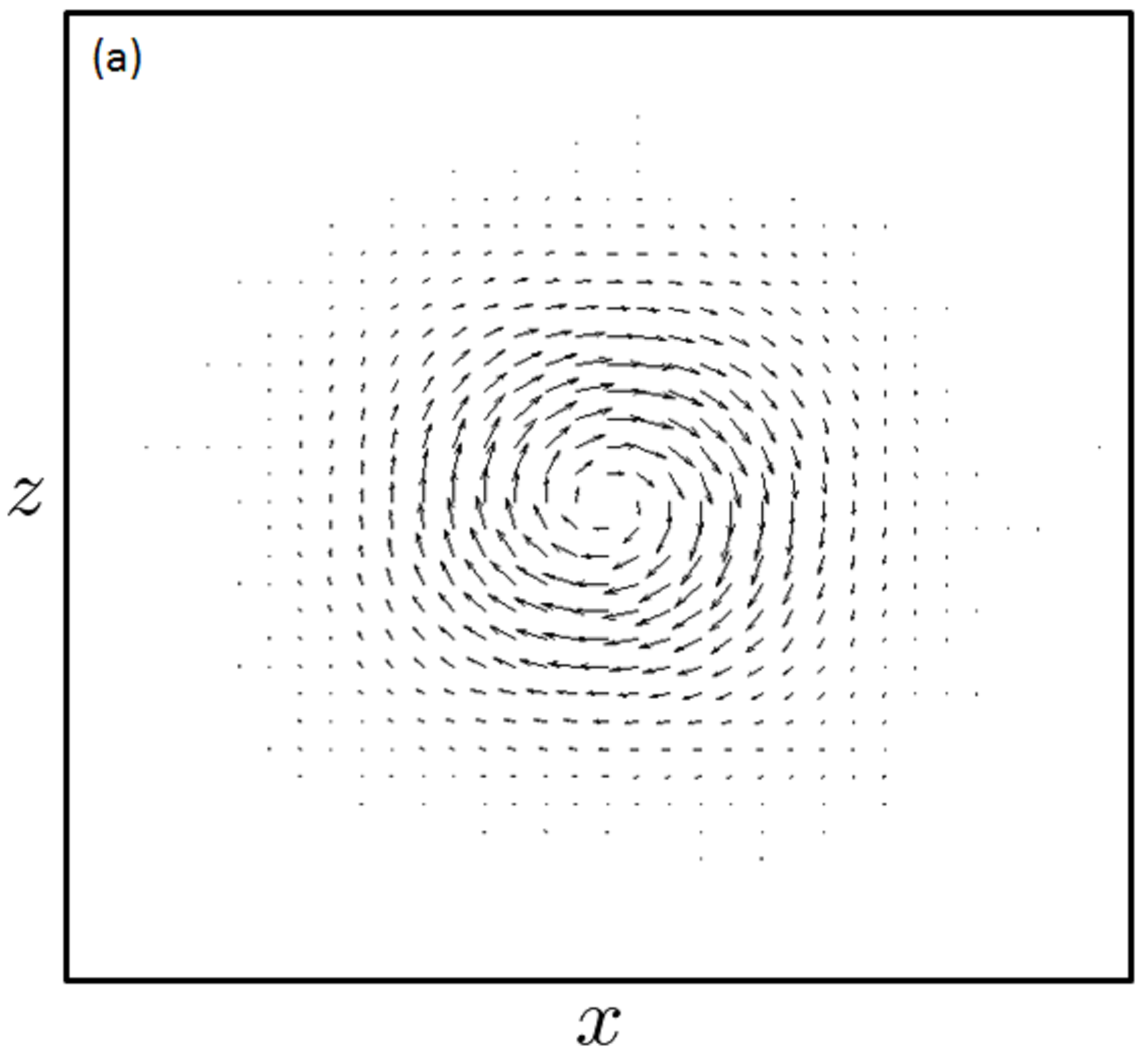
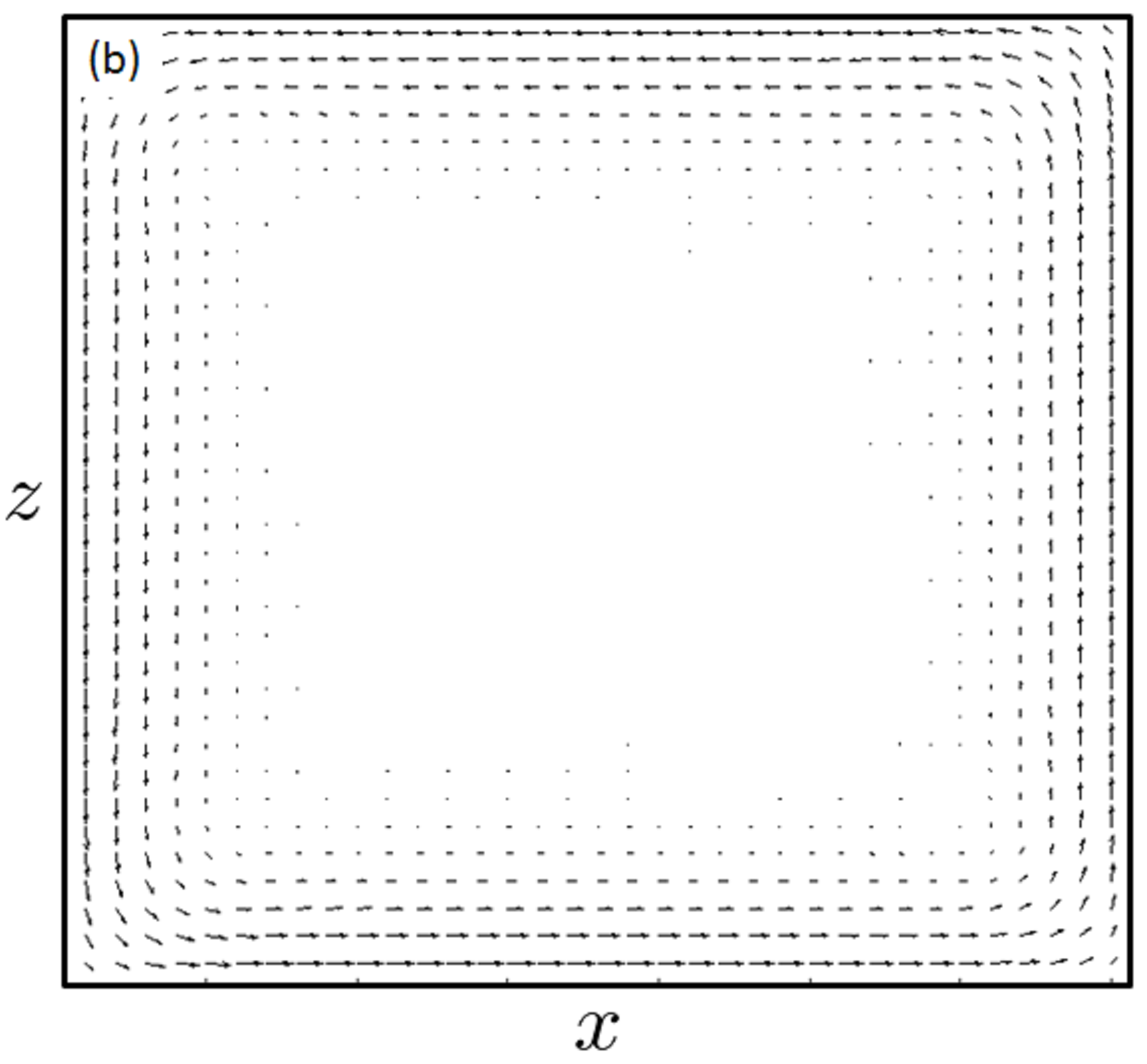
Figure 4: Chiral current vector field for (a) the bulk state in Fig. 2 Eq. (20) and (b) the border state in Fig. 3.

V Conclusion

The present work demonstrates the quantum simulation a Dirac particle in the presence of a magnetic field, putting together quantum simulations of “exotic” dynamics (from the point of view of low-energy physics) and artificial gauge fields. This is intrinsically expected to lead to topological systems, as the Dirac cone is one of the main (and simplest) examples of topology in physics, and opens new ways to explore exciting new possibilities in this very active field. Other interesting prospects would be the inclusion of particle-particle interactions and/or disorder in this analog quantum simulations. These are intriguing and highly challenging tasks, beyond the scope of the present work.

Appendix A Derivation of the Dirac equation

This appendix discusses in more detail the developments leading to Eqs. (8) and (10) for the site amplitudes $c_{n,m}$ and explains how the equations for their continuous envelopes can be put in an form analogous to the Dirac equation. The derivation of the Dirac equation in presence of a gauge field of Sec. III follows the same steps and is also sketched below.

Injecting the general wave function $\psi(x,z,t)=\sum_{n,m}c_{n,m}(t)\exp\left(-i(n\omega_{B}^{(x)}+m\omega_{B}^{(z)})t\right)\varphi_{n}^{(x)}\varphi_{m}^{(z)}$ in the Schrödinger equation for the Hamiltonian $H=H_{0}+\widetilde{V}$ Eq. (6), one obtains the following set of coupled differential equations

$$id_{t}c_{n,m}=\sum_{j,k\in\mathbb{Z}} \left\{\left\langle n,m\right|\widetilde{V}\left|n+j,m+k\right\rangle\right.$$

$$\left.\times\exp\left[-i\left(j\omega_{B}^{(x)}+k\omega_{B}^{(z)}\right)t\right]c_{n+j,m+k}\right\}.$$ (21)

To the dominant order, neglecting non-resonant terms, and keeping nearest neighbor couplings  only $j,k=\pm 1$ in Eq. (21) one gets

$$id_{t}c_{n,m} = -i\frac{V_{x}}{2}\left(\left\langle n,m\right|\cos(2\pi x)\left|n+1,m\right\rangle c_{n+1,m}-\left\langle n,m\right|\cos(2\pi x)\left|n-1,m\right\rangle c_{n-1,m}\right)$$ (22)

$$-i\frac{V_{z}}{2}\left(\left\langle n,m\right|\cos(\pi x)\cos(2\pi z)\left|n,m+1\right\rangle c_{n,m+1}-\left\langle n,m\right|\cos(\pi x)\cos(2\pi z)\left|n,m-1\right\rangle c_{n,m-1}\right).$$

The overlap integrals can be simplified using the Wannier-Stark state translation properties as in Sec. II. For instance:

$$\left\langle n,m\right|\cos(\pi x)\cos(2\pi z)\left|n,m\pm 1\right\rangle =\intop dx\varphi_{n}^{(x)}(x)\varphi_{n}^{(x)}(x)\cos(\pi x)\intop dz\varphi_{m}^{(z)}(x)\varphi_{m\pm 1}^{(z)}(x)\cos(2\pi z)$$

$$=\intop dx\varphi_{0}^{(x)}(x-n)\varphi_{0}^{(x)}(x-n)\cos(\pi x)\intop dz\varphi_{0}^{(z)}(x-m)\varphi_{\pm 1}^{(z)}(x-m)\cos(2\pi z)$$

$$=(-1)^{n}\intop dx\varphi_{0}^{(x)}(x)\varphi_{0}^{(x)}(x)\cos(\pi x)\intop dz\varphi_{0}^{(z)}(x)\varphi_{1}^{(z)}(x)\cos(2\pi z)$$

$$=(-1)^{n}\Omega_{z}$$ (23)

defining the coupling parameter $\Omega_{z}$ [the $(-1)^{n}$ factor come from the perturbation in $\cos(\pi x)$]. The same calculation can be done for overlaps $\left\langle n,m\right|\cos(2\pi x)\left|n\pm 1,m\right\rangle$ and gives

$$\left\langle n,m\right|\cos(2\pi x)\left|n\pm 1,m\right\rangle=\intop dx\varphi_{0}^{(x)}(x)\varphi_{1}^{(x)}(x)\cos(2\pi x)=\Omega_{x}.$$

These results lead to Eq. (8).

When a static perturbation $V_{0}\cos(\pi x)\cos(\pi z)$ is added to Eq. (6), we have, in the resonant approximation, an additional term corresponding to a “self-coupling” contribution

$$V_{0}\left\langle n,m\right|\cos(\pi x)\cos(\pi z)\left|n,m\right\rangle c_{n,m}$$

which is to be added to the R.H.S. of Eq. (8). The overlap integral is then

$$\left\langle n,m\right|\cos(\pi x)\cos(\pi z)\left|n,m\right\rangle = \intop dx\varphi_{n}^{(x)}(x)\varphi_{n}^{(x)}(x)\cos(\pi x)\intop dz\varphi_{n}^{(z)}(x)\varphi_{n}^{(z)}(x)\cos(\pi x)$$

$$= (-1)^{n+m}\intop dx\varphi_{0}^{(x)}(x)\varphi_{0}^{(x)}(x)\cos(\pi x)\intop dz\varphi_{0}^{(z)}(x)\varphi_{0}^{(z)}(x)\cos(\pi x)$$

which in turn gives Eq. (10).

In taking the continuous limit, we have to account for the factors $(-1)^{n}$ and $(-1)^{n+m}$ in Eq. (8) or Eq. (10) which lead to parity-dependent smooth envelopes. Taking as an example $n,m$ even, Eq. (22) shows that $c_{n,m}$ is coupled to the next-neighbors amplitudes with $n$ and $m$ of opposite parities, i.e. $(n\pm 1,m)$ or $(n,m\pm 1)$

$$id_{t}c_{n,m}= T_{0}c_{n,m}+T_{x}\left(c_{n+1,m}-c_{n-1,m}\right)$$

$$+T_{z}\left(c_{n,m+1}-c_{n,m-1}\right),\qquad n,m\;\>\mathrm{even}$$

with the coupling constants $T_{j}=-iV_{j}\Omega_{j}/2$ ($j=x,z$) defined as in Sec. II. Taking the continuous limit $c_{n+1,m}-c_{n-1,m}\simeq 2\partial_{x}c_{oe}$ and $c_{n,m+1}-c_{n,m-1}\simeq 2\partial_{z}c_{eo}$, one has

$$id_{t}s_{ee}(x,z,t) = T_{0}s_{ee}(x,z,t)+2T_{x}\partial_{x}s_{oe}(x,z,t)$$

$$+2T_{z}\partial_{x}s_{eo}(x,z,t)$$

$$= T_{0}s_{ee}(x,z,t)+\Omega_{x}p_{x}s_{oe}(x,z,t)$$

$$+\Omega_{z}p_{z}s_{eo}(x,z,t)$$

where $p_{x}=-i\partial_{x}$, $p_{z}=-i\partial_{z}$. The calculation is analogous for the remaining smooth components $s_{oo},$ $s_{oe}$ and $s_{eo}$.

The introduction of the artificial gauge field in Sec. III follows the same lines as above. The additional modulation terms [see Eq. (11)] generate extra terms in the evolution equation for the amplitudes $c_{n,m}.$ For instance, the term proportional to $V_{x}^{A}z\cos\left(2\pi x\right)\cos(\omega_{B}^{(x)}t)$ gives in the R.H.S. of the evolution equation for amplitudes $c_{n,m}$ the following contribution:

$$\frac{V_{x}^{A}}{2}\left(\left\langle n,m\right|z\cos(2\pi x)\left|n+1,m\right\rangle c_{n+1,m}+\left\langle n,m\right|z\cos(2\pi x)\left|n-1,m\right\rangle c_{n-1,m}\right)$$

$$=\frac{V_{x}^{A}}{2}\left\langle n,m\right|z\cos(2\pi x)\left|n+1,m\right\rangle\left(c_{n+1,m}+c_{n-1,m}\right)$$

with overlap integrals that can then be written as

$$\left\langle n,m\right|z\cos(2\pi x)\left|n\pm 1,m\right\rangle =\Omega_{x}\left\langle m\right|z\left|m\right\rangle$$

$$=\Omega_{x}\intop dzz\left|\varphi_{m}(z)\right|^{2}$$

$$=\Omega_{x}\intop dz(z+m)\left|\varphi_{0}(z)\right|^{2}$$

$$=\Omega_{x}\left\langle\bar{z}+m\right\rangle$$

where the constant $\bar{z}$ is a small offset which can be canceled by a $z$ translation. Equation (12) is then easily obtained, as well as its continuous limit for the envelopes of $c_{ab}$ ($a,b=e,o$), assuming they are smooth enough to allow neglecting second order derivatives (for instance $c_{n+1,m}+c_{n-1,m}\simeq 2s_{ee}(x,z,t)$ for $n$ odd and $m$ even, and so on) .

Appendix B Dirac current

The Dirac equation leads to a standard probability current continuity equation $\partial_{t}\left(\Psi^{\dagger}\Psi\right)+\mathbf{\boldsymbol{\nabla}}\cdot\boldsymbol{j}=0$ with the following current components

$$j_{i}=\left[\Psi\right]^{\dagger}\alpha_{i}\left[\Psi\right]=\phi^{\dagger}\sigma_{i}\chi+\chi^{\dagger}\sigma_{i}\phi$$

where $\left[\Psi\right]=\left[\phi;\chi\right]$ as in Sec. IV. For instance, taking the of Eq. (20) the current is

$$j_{x}\propto-\rho e^{-\rho^{2}}\sin\varphi,\;j_{z}=-\rho e^{-\rho^{2}}\cos\varphi,$$

which is in excellent agreement with Fig. 4(a).

References

• Park et al. (2019) C.-H. Park, L. Yang, Y.-W. Son, M. L. Cohen,  and S. G. Louie, “Anisotropic behaviours of massless Dirac fermions in graphene under periodic potentials,” Nat. Phys. 4, 213–217 (2019).
• Garreau and Zehnlé (2017) J. C. Garreau and V. Zehnlé, “Simulating Dirac models with ultracold atoms in optical lattices,” Phys. Rev. A 96, 043627 (2017).
• Lopez-Gonzalez et al. (2014) X. Lopez-Gonzalez, J. Sisti, G. Pettini,  and M. Modugno, “Effective Dirac equation for ultracold atoms in optical lattices: Role of the localization properties of the Wannier functions,” Phys. Rev. A 89, 033608 (2014).
• Qu et al. (2013) C. Qu, C. Hamner, M. Gong, C. Zhang,  and P. Engels, “Observation of Zitterbewegung in a spin-orbit-coupled Bose-Einstein condensate,” Phys. Rev. A 88, 021604(R) (2013).
• Tarruell et al. (2012) L. Tarruell, D. Greif, T. Uehlinger, G. Jotzu,  and T. Esslinger, “Creating, moving and merging Dirac points with a Fermi gas in a tunable honeycomb lattice,” Nature (London) 483, 302–305 (2012).
• Mazza et al. (2012) L. Mazza, A. Bermudez, N. Goldman, M. Rizzi, M. A. Martin-Delgado,  and M. Lewenstein, “An optical-lattice-based quantum simulator for relativistic field theories and topological insulators,” New J. Phys 14, 015007 (2012).
• Zhang et al. (2012) D.-W. Zhang, Z.-D. Wang,  and S.-L. Zhu, “Relativistic quantum effects of Dirac particles simulated by ultracold atoms,” Front. Phys. 7, 31–53 (2012).
• Gerritsma et al. (2011) R. Gerritsma, B. P. Lanyon, G. Kirchmair, F. Zähringer, C. Hempel, J. Casanova, J. J. García-Ripoll, E. Solano, R. Blatt,  and C. F. Roos, “Quantum Simulation of the Klein Paradox with Trapped Ions,” Phys. Rev. Lett. 106, 060503 (2011).
• Lamata et al. (2011) L. Lamata, J. Casanova, R. Gerritsma, C. F. Roos, J. J. García-Ripoll,  and E. Solano, “Relativistic quantum mechanics with trapped ions,” New J. Phys 13, 095003 (2011).
• Gerritsma et al. (2010) R. Gerritsma, G. Kirchmair, F. Zahringer, E. Solano, R. Blatt,  and C. F. Roos, “Quantum simulation of the Dirac equation,” Nature (London) 463, 68–71 (2010).
• Longhi (2010) S. Longhi, “Photonic analog of Zitterbewegung in binary waveguide arrays,” Opt. Lett. 35, 235–237 (2010).
• Dreisow et al. (2010) F. Dreisow, M. Heinrich, R. Keil, A. Tünnermann, S. Nolte, S. Longhi,  and A. Szameit, “Classical Simulation of Relativistic Zitterbewegung in Photonic Lattices,” Phys. Rev. Lett. 105, 143902 (2010).
• Witthaut et al. (2011) D. Witthaut, T. Salger, S. Kling, C. Grossert,  and M. Weitz, “Effective Dirac dynamics of ultracold atoms in bichromatic optical lattices,” Phys. Rev. A 84, 033601 (2011).
• Feynman (1982) R. P. Feynman, “Simulating Physics with Computers,” Int. J. Theor. Phys. 21, 467–488 (1982).
• Dalibard et al. (2011) J. Dalibard, F. Gerbier, G. Juzeliūnas,  and P. Öhberg, “Artificial gauge potentials for neutral atoms,” Rev. Mod. Phys. 83, 1523–1543 (2011).
• Aidelsburger et al. (2013) M. Aidelsburger, M. Atala, M. Lohse, J. T. Barreiro, B. Paredes,  and I. Bloch, “Realization of the Hofstadter Hamiltonian with Ultracold Atoms in Optical Lattices,” Phys. Rev. Lett. 111, 185301 (2013).
• Galitski and Spielman (2013) V. Galitski and I. B. Spielman, “Spin-orbit coupling in quantum gases,” Nature (London) 494, 49–54 (2013).
• Bloch et al. (2008) I. Bloch, J. Dalibard,  and W. Zwerger, “Many-body physics with ultracold gases,” Rev. Mod. Phys. 80, 885–964 (2008).
• Bloch et al. (2014) I. Bloch, J. Dalibard,  and S. Nascimbene, “Quantum simulations with ultracold quantum gases,” Nat. Phys. 8, 267–276 (2014).
• Georgescu et al. (2014) I. M. Georgescu, S. Ashhab,  and F. Nori, “Quantum simulation,” Rev. Mod. Phys. 86, 153–185 (2014).
• Goldman et al. (2016) N. Goldman, J. C. Budich,  and P. Zoller, “Topological quantum matter with ultracold gases in optical lattices,” Nat. Phys. 12, 639–645 (2016).
• Gross and Bloch (2017) C. Gross and I. Bloch, “Quantum simulations with ultracold atoms in optical lattices,” Science 357, 995–1001 (2017).
• Garreau (2017) J. C. Garreau, “Quantum simulation of disordered systems with cold atoms,” Compt. Rendus Phys. 18, 31 – 46 (2017).
• Note (1) As it will be seen in what follows, this choice makes the writing in terms of the conventional Pauli matrices possible. We will later introduce an artificial magnetic field in the $y$ direction.
• Note (2) We use sans serif characters to represent dimensionfull quantities, except when no ambiguity is possible, e.g. $\hbar$.
• Wannier (1960) G. H. Wannier, “Wave Functions and Effective Hamiltonian for Bloch Electrons in an Electric Field,” Phys. Rev. 117, 432–439 (1960).
• Zener (1934) C. Zener, “A Theory of Electrical Breakdown of Solid Dielectrics,” Proc. R. Soc. (London) A 145, 523—1 (1934).
• Note (3) Experimentally, such linear terms can be obtained by superposing two laser fields of frequencies separated by $\delta\omega$, which generate a beat note varying in space as $\mathop{sin}\nolimits\left(\delta\omega x/c\right)\sim\delta\omega x/c$; if $c/\delta\omega$ is large enough compared to the lattice wavelength the linear approximation can be valid over a large number of neighbor sites where the wavepacket is concentrated.
• Note (4) The Landau gauge can be obtained by setting $T_{z}^{A}=0$ (or $T_{x}^{A}=0$).
• Note (5) We label these solutions “spin up” and “spin down” (with quotation marks) because they are proportional to the eigenstates $(1,\pm i)^{\intercal}/\sqrt{2}$ of $\sigma_{y}$ (remember that $\boldsymbol{B}\parallel\mathbf{y}$). This is not to be confused with spinor-4-particle’s spin components.
• Note (6) Note that these states are also eigenstates of the angular momentum operator $L_{y}+\varSigma_{y}$ , where $\varSigma_{y}=\frac{1}{2}\left(\begin{array}[]{cc}\sigma_{y}&0\\ 0&\sigma_{y}\end{array}\right)$ is the spin operator.
• Note (7) We numerically asserted that a $150\times 150$ lattice gives essentially the same results.
• Peri et al. (2019) V. Peri, M. Serra-Garcia, R. Ilan,  and S. D. Huber, “Axial-field-induced chiral channels in an acoustic Weyl system,” Nat. Phys. 15, 357–361 (2019).
• Wen et al. (2019) X. Wen, C. Qiu, Y. Qi, L. Ye, M. Ke, F. Zhang,  and Z. Liu, “Acoustic Landau quantization and quantum-Hall-like edge states,” Nat. Phys. 15, 352–356 (2019).
• Note (8) This is justified by the rapid vanishing of overlapping integrals between WS states localized in different sites.