A conservative phase-space moving-grid strategy for a 1D-2V Vlasov-Fokker-Planck Equation

Abstract

We develop a conservative phase-space grid-adaptivity strategy for the Vlasov-Fokker-Planck equation in a planar geometry. The velocity-space grid is normalized to the thermal speed and shifted by the bulk-fluid velocity. The configuration-space grid is moved according to a mesh-motion-partial-differential equation (MMPDE), which equidistributes a monitor function that is inversely proportional to the gradient-length scales of the macroscopic plasma quantities. The grid adaptation ensures discrete conservation of the collisional invariants (mass, momentum, and energy). The conservative grid-adaptivity strategy provides an efficient scheme which resolves important physical structures in the phase-space while controlling the computational complexity at all times. We demonstrate the favorable features of the proposed algorithm through a set of test cases of increasing complexity.

1 Introduction

The Vlasov-Fokker-Planck (VFP) collisional kinetic description, coupled with Maxwell’s equations, is regarded as a first-principles physical model for describing weakly coupled plasmas in all collisionality regimes, and accordingly, has a wide range of applications in laboratory (e.g., magnetic and inertial thermonuclear fusion), space (e.g., Earth’s magnetosphere), and astrophysical (e.g., stellar mass ejections) plasmas. In the VFP system, collisions are modeled by the Landau/Rosenbluth-Fokker-Planck collision operator, which describes collisional relaxation of particle-velocity-distribution functions in plasmas under the assumption of binary, grazing-angle collisions [1, 2, 3, 4, 5, 6].

The system of VFP equations for various plasma species supports disparate length and time scales. When coupled with strongly varying (in space and time) plasma temperature, $T$, and bulk-flow velocity, $\mathbf{u}$, this makes the system particularly challenging to solve with Eulerian (grid-based) approaches. The challenges of temperature variation are evident when one considers that the thermal speed, $v_{th}=\sqrt{2T/m}$, provides a characteristic width of the distribution function and is a function of the plasma temperature, $T$, and particle species mass, $m$. In many practical applications of interest (e.g., inertial confinement fusion [ICF]), $v_{th}$ variation for a given species can span several orders of magnitude in both time and space. Also, mass disparities result in strong $v_{th}$ separation for different species. Since the velocity-space domain size is determined by the largest $v_{th}$, and the velocity-space resolution by the smallest $v_{th}$, velocity-space discretization with uniform Cartesian grids in such scenarios may lead to impractical grid-size requirements. To complicate matters further, a large velocity-space domain is required to accommodate the bulk-flow separation in situations where cold, energetic beams interact with a warm thermal background (i.e., $|\mathbf{u}|/v_{th}\gg 1$), further burdening the computational resource requirements.

Several studies have recognized and tried to address these challenges by normalizing the velocity coordinate to the local thermal speed of the plasma and shifting by the bulk flow velocity [7, 8, 9, 10]. In this fashion, the grid expands/contracts as the plasma heats/cools, and shifts as it accelerates/decelerates. Others have considered adaptivity strategies based on either a combination of hierarchical grids [11, 12] by using multiresolution analysis techniques (very much like sparse-grid techniques), or full adaptive-mesh-refinement (AMR) strategies in phase-space [13], providing promising paths for controlling the number of unknowns for Eulerian and semi-Lagrangian schemes. Particularly relevant to this study is the work in Ref. [8], where the velocity-space domain was adapted for multiple ion species based on a single local average $v_{th}$ (over the ion species) and hydrodynamic center-of-mass velocity of the plasma. This powerful strategy enabled the first fully kinetic semi-Lagrangian implosion simulations of inertial confinement fusion (ICF) capsules [8, 14, 15], but required intermittent remapping in both the configuration and velocity space. Unfortunately, all of the strategies outlined above do not conserve mass, momentum, and energy (invariants of the VFP equation) and some also break the structured nature of the grid.

Recently, a novel strategy was proposed in Ref. [16] for a system of 1D-2V Vlasov-Fokker-Planck equations that deals with strong temperature disparity (in both space and time), avoids remapping, and works on structured meshes. The strategy employs a multiple-grid approach by normalizing each species’ velocity to its local and instantaneous thermal speed. The Vlasov-Fokker-Planck equations were transformed analytically and then discretized on a mesh. The transformed equations retained the continuum conservation symmetries, which were then enforced in the discrete via additional nonlinear constraints. This strategy ensures that the species’ distribution functions are always well resolved regardless of temperature or mass disparity. However, this strategy does not allow for species with strongly disparate bulk-flow velocities, ultimately requiring a large number of mesh points in scenarios when $|\mathbf{u}|/v_{th}\gg 1$. Additionally, the evolution of structures in the configuration space was not taken into account, requiring a large number of unknowns to track and resolve sharp features, such as shocks.

In this study, we extend the conservative, multiple-dynamic velocity-space adaptivity strategy in a 1D-2V Cartesian system developed in Ref. [16] to incorporate the further velocity and configuration space (i.e., phase-space) adaptivity discussed above. We consider a quasi-neutral plasma with multiple kinetic ion species and fluid electrons. As before, ionic species are evolved on a velocity-space grid normalized to a temporally and spatially varying characteristic speed, $v^{*}$ (a function of their $v_{th}$), but also shifted by their characteristic velocity, $\mathbf{u}^{*}$ (a function of their $\mathbf{u}$). Also, we evolve the configuration-space coordinate on a logically Cartesian grid, and the Jacobian of the transformation is evolved using a mesh motion partial differential equation (MMPDE) [17, 18, 19]. The approach relies on the equidistribution of monitor functions, which in turn are defined as functions of local gradient-length scales of the plasma. This analytical transformation of the VFP equation introduces additional inertial terms, which are carefully discretized to ensure simultaneous conservation of mass, momentum, and energy.

The rest of the paper is organized as follows. Section 2 introduces the ion-VFP and fluid-electron equations and discusses their conservation properties. In Sec. 3, we introduce the normalized Vlasov-Fokker-Planck equation and detail the coordinate transformation. In Sec. 4, we briefly describe our MMPDE approach, the choice of monitor function, and an algorithm to evolve the configuration-space grid. In Sec. 5, we provide a detailed discussion on the implementation of the proposed scheme in the following order: 1) a discretization of the Vlasov-Fokker-Planck equation with the additional inertial terms, 2) a discretization of the fluid electron temperature equation, 3) a discrete-conservation strategy for the Vlasov component with the added inertial terms, 4) the discretization of our MMPDE equation and the configuration-space grid velocity, and 5) spatial-temporal evolution strategy for $v^{*}$ and $\mathbf{u}^{*}$. The numerical performance of the scheme is demonstrated with various multi-species tests of varying degrees of complexity in Sec. 6. Finally, we conclude in Sec. 7.

2 The System of Vlasov Fokker-Planck ion and fluid electrons equations

A dynamic evolution of weakly-coupled collisional plasmas can be described by a system of Vlasov-Fokker-Planck equation for species $\alpha$ distribution functions (PDF), $f_{\alpha}\left(\mathbf{\mathbf{x},\mathbf{v},t}\right)$, in configuration space, $\mathbf{x}$, velocity space, $\mathbf{v}$, and time, $t$:

$$\partial_{t}f_{\alpha}+\nabla_{x}\cdot\left(\mathbf{v}f_{\alpha}\right)+\frac{q_{\alpha}}{m_{\alpha}}\frac{\partial}{\partial\mathbf{v}}\cdot\left[\left(\mathbf{E}+\mathbf{v}\times\mathbf{B}\right)f_{\alpha}\right]=\sum_{\beta=1}^{N_{s}}C_{\alpha\beta},$$ (2.1)

where $\mathbf{E}$ is the electric field, $\mathbf{B}$ is the magnetic field, $N_{s}$ is the total number of plasma species, and $C_{\alpha\beta}$ is the Fokker-Planck collision operator for species $\alpha$ colliding with species $\beta$:

$$C_{\alpha\beta}=\Gamma_{\alpha\beta}\frac{\partial}{\partial\mathbf{v}}\cdot\left[\stackrel{{\scriptstyle\leftrightarrow}}{{\mathsfsl{D}}}_{\beta}\cdot\nabla_{v}f_{\alpha}-\frac{m_{\alpha}}{m_{\beta}}\mathbf{{A}}_{\beta}f_{\alpha}\right].$$ (2.2)

Here, $\Gamma_{\alpha\beta}=\frac{2\pi Z_{\alpha}^{2}Z_{\beta}^{2}e^{4}\Lambda_{\alpha\beta}}{m_{\alpha}^{2}},$ $\stackrel{{\scriptstyle\leftrightarrow}}{{\mathsfsl{D}}}{}_{\beta}$ and $\mathbf{{A}}_{\beta}$ are the tensor-diffusion and friction coefficients for species $\beta$, $m_{\alpha}$ and $m_{\beta}$ are the masses of species $\alpha$ and $\beta$, respectively, $Z_{\alpha}=q_{\alpha}/e$ is the ionization state of species $\alpha$, $e$ is the proton charge, and $\Lambda_{\alpha\beta}$ is the Coulomb logarithm (unless otherwise specified, $\Lambda_{\alpha\beta}=10$ is assumed for simplicity in this study for all species). In this work, we adopt the Rosenbluth potential formulation [1] to compute $\stackrel{{\scriptstyle\leftrightarrow}}{{\mathsfsl{D}}}_{\beta}$ and $\mathbf{A}_{\beta}$ and refer the readers to Refs. [16, 20, 21] for the detailed numerical treatment of the collision operator.

The collision operator, Eq. (2.2), preserves the positivity of $f_{\alpha}$, and conserves mass, momentum, and energy. The conservation properties stem from the following symmetries [22]:

$$\left<1,C_{\alpha\beta}\right>_{\mathbf{v}} = 0,$$ (2.3)

$$m_{\alpha}\left<\mathbf{v},C_{\alpha\beta}\right>_{\mathbf{v}} = -m_{\beta}\left<\mathbf{v},C_{\beta\alpha}\right>_{\mathbf{v}},$$ (2.4)

$$m_{\alpha}\left<\frac{v^{2}}{2},C_{\alpha\beta}\right>_{\mathbf{v}} = -m_{\beta}\left<\frac{v^{2}}{2},C_{\beta\alpha}\right>_{\mathbf{v}},$$ (2.5)

where the inner product is defined as $\left<A,B\right>_{\mathbf{v}}=2\pi\int_{-\infty}^{\infty}dv_{||}\int_{0}^{\infty}dv_{\perp}v_{\perp}A(\mathbf{v})\,B(\mathbf{v})$ (for the cylindrically symmetric coordinate system in the velocity space employed herein). These conservation symmetries can be enforced in the discrete following the general procedures discussed in Refs. [20, 21].

In this study, we consider a 1D planar geometry in the configuration space without a magnetic field. Without loss of generality and similarly to the previous study [16], we consider a 2V cylindrically symmetric coordinate system in the velocity space. We adopt a fluid-electron model and employ the quasi-neutrality and ambipolarity approximations. We obtain the following simplified system of equations comprised of the ion Vlasov-Fokker-Planck equation (per species $\alpha$),

$$\partial_{t}f_{\alpha}+\partial_{x}\left(v_{||}f_{\alpha}\right)+\frac{q_{\alpha}}{m_{\alpha}}E_{||}\partial_{v_{||}}f_{\alpha}=\sum_{\beta}^{N_{s}}C_{\alpha\beta}+C_{\alpha e}$$ (2.6)

and the electron-temperature equation,

$$\frac{3}{2}\frac{\partial}{\partial t}\left[n_{e}T_{e}\right]+\frac{5}{2}\partial_{x}\left[u_{||,e}n_{e}T_{e}\right]+\partial_{x}Q_{||,e}-q_{e}n_{e}u_{||,e}E_{||}=\sum_{\alpha}^{N_{s}}W_{e\alpha}.$$ (2.7)

Here, $n_{e}=\sum_{\alpha}^{Ns}q_{\alpha}n_{\alpha}$ is the electron number density, $u_{||,e}=\sum_{\alpha}^{N_{s}}q_{\alpha}n_{\alpha}u_{||,\alpha}/n_{e}$ is the parallel electron fluid velocity, and $E_{||}$ is the parallel electric field, evaluated using the Ohm’s law. Also, $Q_{||,e}$ is the parallel electron-heat flux, $T_{e}$ is the electron temperature, $W_{e\alpha}$ describes the electron-ion energy exchange, and the detailed theoretical and numerical treatment of these quantities can be found in [23] and [16], respectively. The electron-ion collision operator $C_{\alpha e}$ in Eq. (2.6) is given by:

$$C_{\alpha e}=\Gamma_{\alpha e}\nabla_{v}\cdot\left[\stackrel{{\scriptstyle\leftrightarrow}}{{\mathsfsl{D}}}_{\alpha e}\cdot\nabla_{v}f_{\alpha}-\frac{m_{\alpha}}{m_{e}}\mathbf{A}_{\alpha e}f_{\alpha}\right],$$ (2.8)

where we adopt the reduced ion-electron potentials [24] (for the full details on the numerics of ensuring discrete conservation, refer to Ref. [16]).

3 Coordinate transformations of the ion Vlasov-Fokker-Planck and fluid-electron equations

We transform the velocity space for a species $\alpha$ by normalizing to a speed, $v_{\alpha}^{*}\left(x,t\right)$, and shifting by a velocity, $u_{||,\alpha}^{*}\left(x,t\right)$, (related to their thermal speed and bulk flow velocity, respectively) as follows:

$$\mathbf{\widetilde{v}}_{\alpha}=\frac{\mathbf{v}}{v_{\alpha}^{*}}-\widehat{u}_{||,\alpha}^{*}\mathbf{e}_{||},\;\frac{\partial}{\partial\widetilde{\mathbf{v}}_{\alpha}}=v_{\alpha}^{*}\frac{\partial}{\partial\mathbf{v}_{\alpha}},\;\widetilde{f}_{\alpha}=\left(v_{\alpha}^{*}\right)^{3}f_{\alpha}.$$

Here, the hat denotes quantities normalized to $v_{\alpha}^{*}$, the tilde denotes quantities additionally shifted by $\widehat{u}_{||,\alpha}^{*}$, and $\mathbf{e}_{||}=\left[1,0,0\right]^{T}$ is the unit vector parallel to the flow direction. To simplify notation, from here on we will denote $\mathbf{v}_{\alpha}$ with $\mathbf{v}$, i.e., we will omit the species subscript. As an example, the density, drift, and temperature moments are defined as:

$$n_{\alpha}=\left\langle 1,\widetilde{f}_{\alpha}\right\rangle_{\widetilde{\mathbf{v}}},\;u_{||,\alpha}=v_{\alpha}^{*}\widehat{u}_{||,\alpha}=v_{\alpha}^{*}\left\langle\widetilde{v}_{||}+\widehat{u}_{||,\alpha}^{*},\widetilde{f}_{\alpha}\right\rangle_{\widetilde{\mathbf{v}}}/n_{\alpha},\;T_{\alpha}=\left(v_{\alpha}^{*}\right)^{2}\widetilde{T}_{\alpha}=\frac{m_{\alpha}\left(v_{\alpha}^{*}\right)^{2}\left\langle\left(\widetilde{\mathbf{v}}+\widehat{u}_{||,\alpha}^{*}-\widehat{u}_{||,\alpha}\right)^{2},{\widetilde{f}}\right\rangle_{\widetilde{\mathbf{v}}}}{3\left\langle 1,{\widetilde{f}}\right\rangle_{\widetilde{\mathbf{v}}}}$$

where $\left\langle\left(\cdot\right),{\widetilde{f}}_{\alpha}\right\rangle_{\widetilde{\mathbf{v}}}=2\pi\int_{-\infty}^{\infty}d{\widetilde{v}}_{||}\int_{0}^{\infty}\left(\cdot\right){\widetilde{f}}_{\alpha}{\widetilde{v}}_{\perp}d{\widetilde{v}}_{\perp}$. The normalization of other relevant quantities and the collision operator with respect to $v_{\alpha}^{*}$ are discussed in Ref. [21]. We note that, as $v_{\alpha}^{*}$ is a function of local $v_{th}$, and $\widehat{u}_{||}^{*}$ a function of the local $u_{||}$ for a given plasma species (elaborated in Sec. 5.5), the grid will expand/contract as the plasma heats/cools, and translates as the plasma accelerates/decelerates. For an illustration of this process, refer to Fig. 3.1.

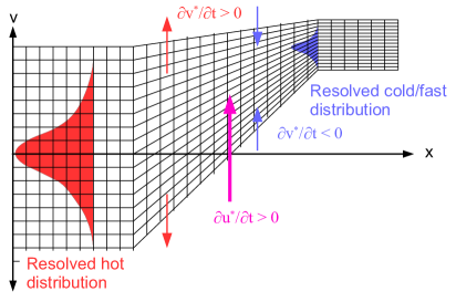
Figure 3.1: Illustration of the velocity space adaptivity.

In the configuration space, we perform a coordinate transformation, $x=x\left(\xi,t\right)$, to evolve the dependent quantities in the logically Cartesian computational space, $\xi$. The Vlasov-Fokker-Planck equation is transformed into the new coordinate system, $\left(\xi,\widetilde{v}_{||},\widetilde{v}_{\perp}\right)$, as follows (details of a derivation are provided in A):

$$\left.\frac{\partial\left(J_{\xi}\widetilde{f}_{\alpha}\right)}{\partial t}\right|_{\xi,\widetilde{\mathbf{v}}}+\frac{\partial}{\partial\xi}\left[\left(v_{\alpha}^{*}\left[\widetilde{v}_{||}+\widehat{u}_{||,\alpha}^{*}\right]-\dot{x}\right)\widetilde{f}_{\alpha}\right]_{\widetilde{\mathbf{v}},t}-\frac{J_{\xi}}{v_{\alpha}^{*}}\frac{\partial}{\partial\widetilde{\mathbf{v}}}\cdot\left[\frac{\partial}{\partial t}\left(v_{\alpha}^{*}\left[\mathbf{\widetilde{v}}+\widehat{u}_{||,\alpha}^{*}\mathbf{e}_{||}\right]\right)\widetilde{f}_{\alpha}\right]_{\xi,t}$$

$$-\frac{1}{v_{\alpha}^{*}}\frac{\partial}{\partial\widetilde{\mathbf{v}}}\cdot\left[\frac{\partial}{\partial\xi}\left(v_{\alpha}^{*}\left[\mathbf{\widetilde{v}}+\widehat{u}_{||,\alpha}^{*}\mathbf{e}_{||}\right]\right)\left(v_{\alpha}^{*}\left[\widetilde{v}_{||}+\widehat{u}_{||,\alpha}^{*}\right]-\dot{x}\right)\widetilde{f}_{\alpha}\right]_{\xi,t}+J_{\xi}\frac{q_{\alpha}}{m_{\alpha}}\frac{E_{||}}{v_{\alpha}^{*}}\left.\frac{\partial\widetilde{f}_{\alpha}}{\partial\widetilde{v}_{||}}\right|_{\xi,t}=J_{\xi}\left[\sum_{\beta}\widetilde{C}_{\alpha\beta}+\widetilde{C}_{\alpha e}\right].$$ (3.1)

Here, $J_{\xi}=\partial_{\xi}x$ is the Jacobian of transformation in the configuration space and $\dot{x}=\partial_{t}x$ is the grid speed. Similarly, the fluid electron temperature equation is given in the transformed coordinate system by:

$$\frac{3}{2}\frac{\partial}{\partial t}\left(J_{\xi}n_{e}T_{e}\right)_{\xi}+\frac{5}{2}\frac{\partial}{\partial\xi}\left(u_{||,e}n_{e}T_{e}\right)_{t}-\frac{3}{2}\frac{\partial}{\partial\xi}\left(\dot{x}n_{e}T_{e}\right)_{t}+\left.\frac{\partial Q_{||,e}}{\partial\xi}\right|_{t}-q_{e}n_{e}u_{||,e}E_{||}J_{\xi}=J_{\xi}\sum_{\alpha}^{N_{sp}}W_{e\alpha}.$$ (3.2)

4 Moving Mesh Partial Differential Equation (MMPDE)

To allow the desired grid adaptivity in the configuration space, we employ a moving-mesh-partial-differential equation (MMPDE) strategy [17, 18, 25, 19]. In particular, we choose the MMPDE5 scheme of Ref. [17],

$$\partial_{t}x=\tau_{x}^{-1}\partial_{\xi}\left[\omega_{x}\partial_{\xi}x\right],$$ (4.1)

with boundary conditions, $\left.x\right|_{\xi=0}=x_{min}$ and $\left.x\right|_{\xi=1}=x_{max}$. Here $\tau_{x}$ is the equilibration time-scale in which the grid reaches an optimal distribution for a given monitor function, $\omega_{x}$ (i.e., for $\tau_{x}\to 0$, we recover $\partial_{\xi}\left[\omega_{x}J_{\xi}\right]=0$), and acts as a temporal smoothing mechanism for the grid evolution. The quality of the grid is governed by the choice of $\omega_{x}$. We choose it to depend on inverse gradient-length scales of $n$, $v_{th}$, and $u_{||}$, and $T_{e}$, and define as:

$$\omega_{x}=\sqrt{\frac{1}{2}\sum_{\alpha}^{N_{sp}}\left[\left(L_{n,\alpha}^{-1}\right)^{2}+\left(L_{v_{th},\alpha}^{-1}\right)^{2}+\left(L_{u_{||},\alpha}^{-1}\right)^{2}\right]+\frac{1}{2}\left(L_{T_{e}}^{-1}\right)^{2}},$$ (4.2)

where, in the discrete, the gradient-length scales are computed as

$$L_{n,\alpha}^{-1}=\left|\frac{\delta_{\xi}n_{\alpha}}{n_{\alpha}}\right|+\delta_{min,n},\;\;\;\;L_{v_{th},\alpha}^{-1}=\left|\frac{\delta_{\xi}v_{th,\alpha}}{v_{th,\alpha}}\right|+\delta_{min,v_{th}},$$ (4.3)

$$L_{u_{||},\alpha}^{-1}=\left|\frac{\delta_{\xi}u_{||,\alpha}}{v_{th,\alpha}}\right|+\delta_{min,u_{||}},\;\;\;\;L_{T_{e}}^{-1}=\left|\frac{\delta_{\xi}T_{e}}{T_{e}}\right|+\delta_{min,T_{e}}.$$

Here, $\delta_{\xi}{\cal M}=0.5\left[{\cal M}\left(\xi+\epsilon_{\xi},t\right)-{\cal M}\left(\xi-\epsilon_{\xi},t\right)\right]$ denotes a finite-differencing operation in the $\xi$ coordinate, where $\epsilon_{\xi}$ is the finite difference factor about point $\xi$, and $\delta_{min,{\cal M}}$ is the floor for the relative variation of the quantity ${\cal M}$. In practical calculations, $\delta_{min,{\cal M}}$ may be individually specified in order to weight the variations of moments separately (e.g., $v_{th}$ and $u_{||}$ variations can be weighted more than variation of $n$ to ensure a smooth grid in velocity space [to be discussed shortly]). In this study, we choose $\delta_{min,{\cal M}}=0.025$ for all ${\cal M}$. Note that, since $u_{||,\alpha}$ is a vector quantity (and therefore can vanish), we normalize it with respect to $v_{th}$. In addition, to avoid an arbitrarily fine mesh, we limit the minimum-to-maximum ratio of the monitor function to a cutoff value, $\eta$, by modifying the monitor function by a constant, $a$,

$$\omega_{x}\leftarrow\omega_{x}+a\;\;\;\textnormal{if}\;\;\;\frac{\omega_{x,min}}{\omega_{x,max}}\leq\eta,$$ (4.4)

where $a=\left(\eta\omega_{x,max}-\omega_{x,min}\right)/\left(1-\eta\right)$ and otherwise stated, $\eta=10^{-2}$ is used in this study. Further, for the stability of the mesh-motion scheme, one must specify a value for $\tau_{x}$ that captures the macroscopic flow evolution well enough while ensuring reasonable grid velocities. Unless otherwise stated, we choose $\tau_{x}=0.5$ in this study, but it can be problem dependent.

5 Numerical Implementation

5.1 Discretization of the VFP equation with inertial terms

Following Refs. [16], we discretize VFP equation, Eq. (3.1), using finite volumes in a 1D planar logical space, $\xi$, and 2V transformed cylindrical-velocity space with azimuthal symmetry, ($\widetilde{v}_{||},\widetilde{v}_{\perp}$). We compute the discrete volume for cell i,j,k (corresponding to logical, parallel, and perpendicular velocity space coordinates, respectively) as:

$$\Delta V_{i,j,k}=J_{\xi,i}\Delta\xi\Delta V_{j,k},$$

with

$$\Delta V_{j,k}=2\pi\widetilde{v}_{\perp,k}\Delta\widetilde{v}_{||}\Delta\widetilde{v}_{\perp},$$

where $J_{\xi,i}=\frac{x_{i+1/2}-x_{i-1/2}}{\Delta\xi}$ is the discrete Jacobian in the configuration space, and $\Delta\xi$, $\Delta{\widetilde{v}}_{||}$, and $\Delta{\widetilde{v}}_{\perp}$ are the mesh spacings in the logical and the transformed parallel- and perpendicular-velocity spaces, respectively. For uniform logical and normalized velocity-space meshes, we have:

$$\Delta\xi=\frac{1}{N_{\xi}},\,\,\Delta{\widetilde{v}}_{||}=\frac{\widetilde{L}_{||}}{N_{||}},\,\,\Delta{\widetilde{v}}_{\perp}=\frac{\widetilde{L}_{\perp}}{N_{\perp}},$$

where, $\widetilde{L}_{||}$ and $\widetilde{L}_{\perp}$ are the normalized parallel and perpendicular velocity-space domain sizes, respectively; and $N_{\xi}$, $N_{||}$, and $N_{\perp}$ are the corresponding numbers of cells. The mesh is arranged such that cell faces map to the domain boundary (and therefore outermost cell centers are half a mesh-spacing away from the boundary). We define the distribution function $f$ at cell centers.

Velocity-space inner products are approximated via a mid-point quadrature rule as

$$\left<A,B\right>_{\widetilde{\mathbf{v}}}\approx\left<A,B\right>_{\delta\widetilde{\mathbf{v}}}=\sum_{j=1}^{N_{||}}\sum_{k=1}^{N_{\perp}}A_{j,k}B{}_{j,k}\Delta V_{j,k}$$ (5.1)

for scalars, and

$$\left<\mathbf{A},\mathbf{B}\right>_{\widetilde{\mathbf{v}}}\approx\left<\mathbf{A},\mathbf{B}\right>_{\delta\widetilde{\mathbf{v}}}=$$

$$2\pi\left[\sum_{j=0}^{N_{||}}\sum_{k=1}^{N_{\perp}}\widetilde{v}_{\perp,k}\Delta\widetilde{v}_{||}\Delta\widetilde{v}_{\perp}A_{||,j+1/2,k}B{}_{||,j+1/2,k}+\sum_{j=1}^{N_{||}}\sum_{k=0}^{N_{\perp}}\widetilde{v}_{\perp,k+1/2}\Delta\widetilde{v}_{||}\Delta\widetilde{v}_{\perp}A_{\perp,j,k+1/2}B{}_{\perp,j,k+1/2}\right]$$ (5.2)

for vectors (with their components at cell faces denoted by the half-integer indices $j+1/2$, $k+1/2$).

We discretize Eq. (3.1) in a conservative form as

$$\frac{c^{(p+1)}J_{\xi,i}^{(p+1)}\widetilde{f}_{\alpha,i,j,k}^{(p+1)}+c^{(p)}J_{\xi,i}^{(p)}\widetilde{f}_{\alpha,i,j,k}^{(p)}+c^{(p-1)}J_{\xi,i}^{(p-1)}\widetilde{f}_{\alpha,i,j,k}^{(p-1)}}{\Delta t^{(p)}}$$

$$+\underbrace{\frac{F_{x,\alpha,i+1/2,j,k}^{(p+1)}-F_{x,\alpha,i-1/2,j,k}^{(p+1)}}{\Delta\xi}}_{ⓐ}+\underbrace{\frac{F_{\dot{x},\alpha,i+1/2,j,k}^{(p+1)}-F_{\dot{x},\alpha,i-1/2,j,k}^{(p+1)}}{\Delta\xi}}_{ⓑ}+\underbrace{\frac{J_{\alpha,acc,i,j+1/2,k}^{(p+1)}-J_{\alpha,acc,i,j-1/2,k}^{(p+1)}}{\Delta\widetilde{v}_{||}}}_{ⓒ}$$ (5.3)

$$+\underbrace{\left[\frac{J_{||,t,\alpha,i,j+1/2,k}^{(p+1)}-J_{||,t,\alpha,i,j-1/2,k}^{(p+1)}}{\Delta\widetilde{v}_{||}}+\frac{\widetilde{v}_{\perp,k+1/2}J_{\perp,t,\alpha,i,j,k+1/2}^{(p+1)}-\widetilde{v}_{\perp,k-1/2}J_{\perp,t,\alpha,i,j,k-1/2}^{(p+1)}}{\widetilde{v}_{\perp,k}\Delta\widetilde{v}_{\perp}}\right]}_{ⓓ}$$

$$+\underbrace{\left[\frac{J_{||,x,\alpha,i,j+1/2,k}^{(p+1)}-J_{||,x,\alpha,i,j-1/2,k}^{(p+1)}}{\Delta\widetilde{v}_{||}}+\frac{\widetilde{v}_{\perp,k+1/2}J_{\perp,x,\alpha,i,j,k+1/2}^{(p+1)}-\widetilde{v}_{\perp,k-1/2}J_{\perp,x,\alpha,i,j,k-1/2}^{(p+1)}}{\widetilde{v}_{\perp,k}\Delta\widetilde{v}_{\perp}}\right]}_{ⓔ}$$

$$=J_{\xi,i}^{(p+1)}\left[\sum_{\beta}^{N_{s}}\left.\widetilde{C}_{\alpha\beta}^{(p+1)}\right|_{i,j,k}+\left.\widetilde{C}_{\alpha e}^{(p+1)}\right|_{i,j,k}\right].$$ (5.4)

Here, $c^{(p+1)}$, $c^{(p)}$, and $c^{(p-1)}$ are the coefficients for the second-order backwards difference formula (BDF2) [26] and superscripts $(p)$ is the discrete time index.

The term $ⓐ$ corresponds to the discretization of the spatial streaming term, with

$$F_{x,\alpha,i+1/2,j,k}^{(p+1)}=v_{\alpha,i+1/2}^{*,(p)}\left(\widetilde{v}_{||,j}+\widehat{u}_{||,\alpha,i+1/2}^{*,(p)}\right)\textnormal{Interp}\left(\widetilde{v}_{||,j}+\widehat{u}_{||,\alpha,i+1/2}^{*,(p)},\widetilde{f}_{\alpha}^{(p+1)}\right)_{i+1/2,j,k},$$ (5.5)

$$v_{\alpha,i+1/2}^{*,(p)}=\frac{v_{\alpha,i+1}^{*,(p)}+v_{\alpha,i}^{*,(p)}}{2},\;\textnormal{and}\;\widehat{u}_{||,\alpha,i+1/2}^{*,(p)}=\frac{\widehat{u}_{||,\alpha,i}^{*,(p)}+\widehat{u}_{||,\alpha,i+1}^{*,(p)}}{2},$$

where $\textnormal{Interp}\left(a,\phi\right)_{face}$ is an advection interpolation operator of a scalar $\phi$ at a cell face with a given velocity $a$, which can be written in general as

$$\textnormal{Interp}\left(a,\phi\right)_{face}=\sum_{i^{\prime}=1}^{N}\omega_{face,i^{\prime}}\left(a,\phi\right)\phi_{i^{\prime}}.$$ (5.6)

The coefficients $\omega_{face,i^{\prime}}$ are the interpolation weights for the spatial cells $i^{\prime}$ surrounding the cell face of interest. In this study, they are determined by the SMART discretization [27], which ensures the positivity of the solution and is well-posed for nonlinear iterative methods.

The term $ⓑ$ corresponds to the inertial term in the configuration space, arising from the moving grid, with

$$F_{\dot{x},\alpha,i+1/2,j,k}^{(p+1)}=-\dot{x}_{i+1/2}^{(p+1)}\textnormal{Interp}\left(-\dot{x}_{i+1/2}^{(p+1)},\widetilde{f}_{\alpha}^{(p+1)}\right)_{i+1/2,j,k},$$ (5.7)

where the definition of $\dot{x}_{i+1/2}$ is given in Sec. 5.4.

The term $ⓒ$ corresponds to the electrostatic-acceleration term with

$$J_{\alpha,acc,i,j+1/2,k}^{(p+1)}=J_{\xi}\frac{q_{\alpha}}{m_{\alpha}}\frac{E_{||,i}^{(p+1)}}{v_{\alpha,i}^{*,p}}\textnormal{Interp}\left(q_{\alpha}E_{||,i}^{(p+1)},\widetilde{f}_{\alpha}^{(p+1)}\right)_{i,j+1/2,k}.$$ (5.8)

The term $ⓓ$ corresponds to the inertial terms due to temporal variation of the velocity space metrics (i.e., $v_{\alpha}^{*}$ and $\widehat{u}_{||,\alpha}^{*}$) with

$$J_{||,t,\alpha,i,j+1/2,k}^{(p+1)}=\gamma_{t,\alpha,i,j+1/2,k}^{(p+1)}{\cal I}_{||,t,\alpha,i,j+1/2,k}^{(p)}\textnormal{Interp}\left({\cal I}_{||,t,\alpha,i+1/2,j+1/2,k}^{(p+1)},\widetilde{f}_{\alpha}^{(p+1)}\right)_{i,j+1/2,k}$$ (5.9)

and

$$J_{\perp,t,\alpha,i,j,k+1/2}^{(p+1)}=\gamma_{t,\alpha,i,j,k+1/2}^{(p+1)}{\cal I}_{\perp,t,\alpha,i,j,k+1/2}^{(p+1)}\textnormal{Interp}\left({\cal I}_{\perp,t,\alpha,i,j,k+1/2}^{(p+1)},\widetilde{f}_{\alpha}^{(p+1)}\right)_{i,j,k+1/2},$$ (5.10)

where $\gamma_{t,\alpha}=\gamma_{t,\alpha}\left(\xi,\widetilde{\mathbf{v}}\right)$ is the discrete nonlinear constraint function that enforces the simultaneous momentum- and energy-conservation symmetries arising from the temporal variations of the metrics (to be discussed shortly),

$${\cal I}_{||,t,\alpha,i,j+1/2,k}^{(p+1)}=-\left[\frac{J_{\xi,i}^{(p+1)}}{v_{\alpha,i}^{*,(p)}}\frac{\partial}{\partial t}\left(v_{\alpha}^{*}\left[\widetilde{v}_{||,j+1/2}+\widehat{u}_{||,\alpha}^{*}\right]\right)_{i}^{(p+1)}\right]\approx$$

$$-\frac{J_{\xi,i}^{(p+1)}}{v_{\alpha,i}^{*,(p)}\Delta t^{(p)}}\left[c^{(p+1)}v_{\alpha,i}^{*,(p)}\left(\widetilde{v}_{||,j+1/2}+\widehat{u}_{||,\alpha,i}^{*,(p)}\right)+c^{(p)}v_{\alpha,i}^{*,(p-1)}\left(\widetilde{v}_{||,j+1/2}+\widehat{u}_{||,\alpha,i}^{*,(p-1)}\right)\right.$$ (5.11)

$$\left.+c^{(p-1)}v_{\alpha,i}^{*,(p-2)}\left(\widetilde{v}_{||,j+1/2}+\widehat{u}_{||,\alpha,i}^{*,(p-2)}\right)\right]$$ (5.12)

and

$${\cal I}_{\perp,t,\alpha,i,j,k+1/2}^{(p+1)}=-\frac{J_{\xi,i}^{(p+1)}}{v_{\alpha,i}^{*,(p)}}\left[\frac{\partial}{\partial t}\left(v_{\alpha}^{*}\widetilde{v}_{\perp}\right)_{i,k+1/2}^{(p+1)}\right]\approx-\frac{J_{\xi,i}^{(p+1)}}{v_{\alpha,i}^{*,(p)}}\left[\frac{c^{(p+1)}v_{\alpha,i}^{*,(p)}+c^{(p)}v_{\alpha,i}^{*,(p-1)}+c^{(p-1)}v_{\alpha,i}^{*,(p-2)}}{\Delta t^{(p)}}\widetilde{v}_{\perp,k+1/2}\right].$$ (5.13)

As described in Ref. [21], we lag the time level between the BDF2 coefficients and the normalization speed (and similarly, the shift velocity) to avoid over-constraining the nonlinear residual (see the reference for further detail).

The term $ⓔ$ corresponds to the inertial terms due to the spatial variation of the metrics with

$$J_{||,x,\alpha,i,j+1/2,k}^{(p+1)}=0.5\left[J_{||,x,\alpha,i+1/2,j+1/2,k}^{(p+1),-}+J_{||,x,\alpha,i-1/2,j+1/2,k}^{(p+1),+}\right]$$ (5.14)

$$J_{\perp,x,\alpha,i,j,k+1/2}^{(p+1)}=0.5\left[J_{\perp,x,\alpha,i+1/2,j,k+1/2}^{(p+1),-}+J_{\perp,x,\alpha,i-1/2,j,k+1/2}^{(p+1),+}\right],$$ (5.15)

where

$$J_{||,x,\alpha,i\pm 1/2,j+1/2,k}^{(p+1),\mp}=\gamma_{x,i\pm 1/2,j+1/2,k}^{(p+1)}{\cal I}_{||,x,\alpha,i\pm 1/2,j+1/2,k}^{(p+1),\mp}\textnormal{Interp}\left({\cal I}_{||,x,\alpha,i\pm 1/2,j+1/2,k}^{(p+1),\mp},\widetilde{f}_{\alpha}^{(p+1)}\right)_{i,j+1/2,k}$$ (5.16)

and

$$J_{\perp,x,\alpha,i\pm 1/2,j,k+1/2}^{(p+1),\mp}=\gamma_{x,i\pm 1/2,j,k+1/2}^{(p+1)}{\cal I}_{\perp,x,\alpha,i\pm 1/2,j,k+1/2}^{(p+1),\mp}\textnormal{Interp}\left({\cal I}_{\perp,x,\alpha,i\pm 1/2,j,k+1/2}^{(p+1),\mp},\widetilde{f}_{\alpha}^{(p+1)}\right)_{i,j,k+1/2}.$$ (5.17)

Here, similarly to $\gamma_{t}$, $\gamma_{x}=\gamma_{x}\left(\xi,\widetilde{\mathbf{v}}\right)$ is the discrete nonlinear constraint function which enforces the simultaneous mass, momentum, and energy conservation symmetries arising from the coordinate transformation,

$${\cal I}_{||,x,\alpha,i+1/2,j+1/2,k}^{(p+1),\mp}=-\frac{1}{v_{\alpha,i+1/2}^{*,\mp}}\left\{\left[v_{\alpha}^{*}\left(\widetilde{v}_{||}+\widehat{u}_{||,\alpha}^{*}\right)-\dot{x}\right]\frac{\partial}{\partial\xi}\left[v_{\alpha}^{*}\left(\widetilde{v}_{||}+\widehat{u}_{||,\alpha}^{*}\right)\right]\right\}_{i+1/2,j+1/2,k}^{(p+1)}$$

$$\approx-\frac{v_{\alpha,i+1/2}^{*,(p)}\left(\widetilde{v}_{||,j+1/2}+\widehat{u}_{||,\alpha,i+1/2}^{*,(p)}\right)-\dot{x}_{i+1/2}^{(p+1)}}{v_{\alpha,i+1/2\mp 1/2}^{*,(p)}}\frac{v_{\alpha,i+1}^{*,(p)}\left(\widetilde{v}_{||,j+1/2}+\widehat{u}_{||,\alpha,i+1}^{*,(p)}\right)-v_{\alpha,i}^{*,(p)}\left(\widetilde{v}_{||,j+1/2}+\widehat{u}_{||,\alpha,i}^{*,(p)}\right)}{\Delta\xi}$$ (5.18)

and

$${\cal I}_{\perp,x,\alpha,i+1/2,j,k+1/2}^{(p),\mp}=-\frac{1}{v_{\alpha,i+1/2\mp 1/2}^{*}}\left\{\left[v_{\alpha}^{*}\left(\widetilde{v}_{||}+\widehat{u}_{||,\alpha}^{*}\right)-\dot{x}\right]\frac{\partial}{\partial\xi}\left(v_{\alpha}^{*}\widetilde{v}_{\perp}\right)\right\}_{i+1/2,j,k+1/2}^{(p+1)}$$

$$\approx-\frac{v_{\alpha,i+1/2}^{*,(p)}\left(\widetilde{v}_{||,j}+\widehat{u}_{||,\alpha,i+1/2}^{*,(p)}\right)-\dot{x}_{i+1/2}^{(p+1)}}{v_{\alpha,i+1/2\mp 1/2}^{*,(p)}}\frac{v_{\alpha,i+1}^{*,(p)}\widetilde{v}_{\perp,k+1/2}-v_{\alpha,i}^{*,(p)}\widetilde{v}_{\perp,k+1/2}}{\Delta\xi}.$$ (5.19)

Finally, the right-hand-side of Eq. (5.4) corresponds to the Fokker-Planck collision operator and its treatment is discussed in detail in Refs. [20, 21]. In this study, we use the Du Toit-O’Brien-Vann (DOV) differencing scheme [28] for the tensor diffusion operator in the collision term to cast the off-diagonal component of this operator as a nonlinear advection term. This strategy allows the use of many high-order, maximum-principle-preserving discretization schemes (e.g., SMART) and simplifies the preconditioning strategy (i.e., upwind differencing can be used for this term).

5.2 Discretization of the Fluid Electron Equation

The electron temperature equation in the transformed coordinate system, Eq. (3.2), is discretized using a finite-volume scheme in space and BDF2 in time:

$$\frac{3}{2}\frac{c^{(p+1)}J_{\xi,i}^{(p+1)}n_{e,i}^{(p+1)}T_{e,i}^{(p+1)}+c^{(p)}J_{\xi,i}^{(p)}n_{e,i}^{(p)}T_{e,i}^{(p)}+c^{(p-1)}J_{\xi,i}^{(p-1)}n_{e,i}^{(p-1)}T_{e,i}^{(p-1)}}{\Delta t^{(p)}}+$$

$$\frac{5}{2}\frac{u_{||,e,i+1/2}^{(p+1)}\left(\widetilde{n_{e}T_{e}}\right)_{i+1/2}^{(p+1)}-u_{||,e,i-1/2}^{(p+1)}\left(\widetilde{n_{e}T_{e}}\right)_{i-1/2}^{(p+1)}}{\Delta\xi}-\frac{3}{2}\frac{\dot{x}_{i+1/2}^{(p+1)}\left(\widetilde{n_{e}T_{e}}\right)_{i+1/2}^{(p+1)}-\dot{x}_{i-1/2}^{(p+1)}\left(\widetilde{n_{e}T_{e}}\right)_{i-1/2}^{(p+1)}}{\Delta\xi}+$$ (5.20)

$$\frac{Q_{||,e,i+1/2}^{(p+1)}-Q_{||,e,i-1/2}^{(p+1)}}{\Delta\xi}-q_{e}\left[n_{e}u_{||,e}E_{||}\right]_{i}^{(p+1)}J_{\xi,i}^{(p+1)}=$$ (5.21)

$$\left[3\nu_{e\alpha,i}^{(p+1)}\frac{m_{e}}{m_{\alpha}}n_{e,i}^{(p+1)}\left(T_{\alpha,i}^{(p+1)}-T_{e,i}^{(p+1)}\right)-F_{||,\alpha e,i}^{(p+1)}u_{||,\alpha,i}^{(p+1)}\right]J_{\xi,i}^{(p+1)}.$$ (5.22)

Here, the tilde denotes a cell-face discretization for the advection quantities (SMART in this study). The Joule-heating quantity (last term on the left-hand-side) is defined so as to enforce conservation properties in the discrete with the detailed expression as well as treatment of all other terms provided in Ref. [16].

5.3 Discretization of the Vlasov component: exact conservation properties

This section describes the procedure to ensure the set of exact conservation symmetries of the Vlasov piece in the ion kinetic equation in the presence of phase-space grid adaptivity. In this, we follow a procedure similar to that discussed in Refs. [21, 16], but with significant simplification in the derivation of the symmetries. We note that the conservation properties associated with the temporal and spatial variation of metrics can be shown independently. We begin by developing discretizations for fully mass, momentum, and energy conservation in spatially homogeneous system (0D), and then a spatially inhomegenous case (1D) in a periodic spatial domain without any background field (conservation with electric field can be shown separately, as shown in Ref. [16]).

5.3.1 Temporal variation of $v^{*}$ and $\widehat{u}_{||}^{*}$

If we consider only the terms associated with the temporally varying metrics in Eq. (3.1) (i.e., a homogeneous plasma), we obtain the following simplified form of the Vlasov equation:

$$\partial_{t}\left(J_{\xi}\widetilde{f}\right)_{\xi,\widetilde{\mathbf{v}}}-\frac{J_{\xi}}{v^{*}}\frac{\partial}{\partial\widetilde{\mathbf{v}}}\cdot\left(\left.\partial_{t}\mathbf{v}\right|_{\xi,\widetilde{\mathbf{v}}}\widetilde{f}\right)_{\xi,t}=0,$$ (5.23)

where $\partial_{t}\left.\mathbf{v}\right|_{\xi,\widetilde{\mathbf{v}}}=\partial_{t}\left[v^{*}\left(\mathbf{\widetilde{v}}+\widehat{u}_{||}^{*}\mathbf{e}_{||}\right)\right]_{\xi,\widetilde{\mathbf{v}}}$. In the continuum, mass conservation is defined as:

$$\int_{0}^{1}d\xi\left\langle m,\partial_{t}\left(J_{\xi}\widetilde{f}\right)\right\rangle_{\widetilde{\mathbf{v}}}=0.$$ (5.24)

This can be shown trivially due to the divergence form of the inertial terms.

Momentum conservation is defined as

$$\int_{0}^{1}d\xi\left\langle m,\partial_{t}\left(v_{||}J_{\xi}\widetilde{f}\right)\right\rangle_{\widetilde{\mathbf{v}}}=0.$$ (5.25)

This can be shown (for brevity, dropping the explicit integration in $\xi$) by multiplying Eq. (5.23) by $mv_{||}$, and using the chain rule to obtain:

$$m\left\{\partial_{t}\left(v_{||}J_{\xi}{\widetilde{f}}\right)_{\xi,\widetilde{\mathbf{v}}}-\left[\underbrace{J_{\xi}{\widetilde{f}}\partial_{t}\left.v_{||}\right|_{\xi,\widetilde{v}_{||}}}_{ⓐ}+\underbrace{\frac{J_{\xi}v_{||}}{v^{*}}\frac{\partial}{\partial\widetilde{\mathbf{v}}}\cdot\left(\left.\partial_{t}\mathbf{v}\right|_{\xi,\widetilde{\mathbf{v}}}\widetilde{f}\right)_{\xi,t}}_{ⓑ}\right]\right\}=0.$$

Taking $\left\langle 1,\left(\cdot\right)\right\rangle_{\widetilde{\mathbf{v}}}$ of above, the terms $ⓐ$ and $ⓑ$ yields:

$$\left\langle 1,ⓐ\right\rangle_{\widetilde{\mathbf{v}}}=J_{\xi}\left\langle\left.\partial_{t}v_{||}\right|_{\xi,\widetilde{v}_{||}},\widetilde{f}\right\rangle_{\widetilde{\mathbf{v}}},$$

$$\left\langle 1,ⓑ\right\rangle_{\widetilde{\mathbf{v}}}=J_{\xi}\left\langle\frac{v_{||}}{v^{*}},\frac{\partial}{\partial\mathbf{\widetilde{v}}}\cdot\left(\left.\partial_{t}\mathbf{v}\right|_{\xi,\widetilde{\mathbf{v}}}\widetilde{f}\right)_{\xi,t}\right\rangle_{\widetilde{\mathbf{v}}}=-J_{\xi}\left\langle\left.\partial_{t}v_{||}\right|_{\xi,\widetilde{v}_{||}},\widetilde{f}\right\rangle_{\widetilde{\mathbf{v}}},$$

canceling each other and leaving $\left\langle m,\partial_{t}\left(v_{||}J_{\xi}\widetilde{f}\right)_{\xi,\widetilde{\mathbf{v}}}\right\rangle_{\widetilde{\mathbf{v}}}=0$. Thus, the key is to ensure that in the discrete we satisfy the following relation:

$$\left\langle v_{||},\partial_{t}\left(J_{\xi}\widetilde{f}\right)_{\xi,\widetilde{\mathbf{v}}}-\frac{J_{\xi}}{v^{*}}\frac{\partial}{\partial\widetilde{\mathbf{v}}}\cdot\left(\left.\partial_{t}\mathbf{v}\right|_{\xi,\widetilde{\mathbf{v}}}\widetilde{f}\right)_{\xi,t}\right\rangle_{\mathbf{\widetilde{v}}}=\left\langle 1,\partial_{t}\left(v_{||}J_{\xi}\widetilde{f}\right)_{\xi,\widetilde{\mathbf{v}}}\right\rangle_{\mathbf{\widetilde{v}}}.$$ (5.26)

Similarly, energy conservation is defined as

$$\int_{0}^{1}d\xi\left\langle m,\partial_{t}\left(\frac{v^{2}}{2}J_{\xi}\widetilde{f}\right)\right\rangle_{\widetilde{\mathbf{v}}}=0.$$ (5.27)

This can be shown by multiplying Eq. (5.23) by $m\frac{v^{2}}{2}$, and using the chain rule to obtain:

$$m\left\{\partial_{t}\left(\frac{v^{2}}{2}J_{\xi}{\widetilde{f}}\right)_{\xi,\widetilde{\mathbf{v}}}-\left[\underbrace{J_{\xi}{\widetilde{f}}\partial_{t}\left.\frac{v^{2}}{2}\right|_{\xi,\widetilde{\mathbf{v}}}}_{ⓐ}+\underbrace{\frac{J_{\xi}v^{2}}{2v^{*}}\frac{\partial}{\partial\widetilde{\mathbf{v}}}\cdot\left(\left.\partial_{t}\mathbf{v}\right|_{\xi,\widetilde{\mathbf{v}}}\widetilde{f}\right)_{\xi,t}}_{ⓑ}\right]\right\}=0.$$

Taking $\left\langle 1,\left(\cdot\right)\right\rangle_{\widetilde{\mathbf{v}}}$ of above, the terms $ⓐ$ and $ⓑ$ yields:

$$\left\langle 1,ⓐ\right\rangle_{\widetilde{\mathbf{v}}}=J_{\xi}\left\langle\left.\partial_{t}\frac{v^{2}}{2}\right|_{\xi,\widetilde{\mathbf{v}}},\widetilde{f}\right\rangle_{\widetilde{\mathbf{v}}},$$

$$\left\langle 1,ⓑ\right\rangle_{\widetilde{\mathbf{v}}}=J_{\xi}\left\langle\frac{v^{2}}{2v^{*}},\frac{\partial}{\partial\mathbf{\widetilde{v}}}\cdot\left(\left.\partial_{t}\mathbf{v}\right|_{\xi,\widetilde{\mathbf{v}}}\widetilde{f}\right)_{\xi,t}\right\rangle_{\widetilde{\mathbf{v}}}=-J_{\xi}\left\langle\mathbf{v},\left.\partial_{t}\mathbf{v}\right|_{\xi,\widetilde{\mathbf{v}}}\widetilde{f}\right\rangle_{\widetilde{\mathbf{v}}}=-J_{\xi}\left\langle\left.\partial_{t}\frac{v^{2}}{2}\right|_{\xi,\widetilde{\mathbf{v}}},\widetilde{f}\right\rangle_{\widetilde{\mathbf{v}}},$$

canceling each other and leaving $\left\langle m,\partial_{t}\left(\frac{v^{2}}{2}J_{\xi}\widetilde{f}\right)_{\xi,\widetilde{\mathbf{v}}}\right\rangle_{\widetilde{\mathbf{v}}}=0$. Thus, the key is to ensure that in the discrete, we satisfy the following relation:

$$\left\langle\frac{v^{2}}{2},\partial_{t}\left(J_{\xi}\widetilde{f}\right)_{\xi,\widetilde{\mathbf{v}}}-\frac{J_{\xi}}{v^{*}}\frac{\partial}{\partial\widetilde{\mathbf{v}}}\cdot\left(\left.\partial_{t}\mathbf{v}\right|_{\xi,\widetilde{\mathbf{v}}}{\widetilde{f}}\right)_{\xi,t}\right\rangle_{\widetilde{\mathbf{v}}}=\left\langle 1,\partial_{t}\left(\frac{v^{2}}{2}J_{\xi}\widetilde{f}\right)_{\xi,\widetilde{\mathbf{v}}}\right\rangle_{\widetilde{\mathbf{v}}}.$$ (5.28)

In the discrete, the symmetries given by Eqs. (5.26) and (5.28) are not satisfied automatically due to truncation error, ${\cal O}\left(\Delta_{v}^{\beta},\Delta_{t}^{\zeta}\right)$, where $\beta$ and $\zeta$ denote the order of discretization in the velocity space and time, respectively. We ensure them by multiplying the inertial term by a velocity-space dependent function, $\gamma_{t}\left(\mathbf{v}\right)$, such that, at a time-step $p$,

$$\left\langle v_{||,i}^{(p)},\delta_{\widetilde{\mathbf{v}}}\cdot\left(\gamma_{t,i}^{(p+1)}\underbrace{J_{\xi,i}^{(p+1)}\left[v_{i}^{*,(p)}\right]^{-1}\delta_{t}\mathbf{v}_{i}^{(p+1)}}_{ⓐ}\widetilde{f}_{i}^{(p+1)}\right)\right\rangle_{\delta\mathbf{\widetilde{v}}}-$$ (5.29)

$$\left[\left\langle v_{||,i}^{(p)},\delta_{t}\left(J_{\xi}\widetilde{f}\right)_{i}^{(p+1)}\right\rangle_{\delta\mathbf{\widetilde{v}}}-\left\langle 1,\delta_{t}\left(v_{||}J_{\xi}\widetilde{f}\right)_{i}^{(p+1)}\right\rangle_{\delta\mathbf{\widetilde{v}}}\right]=0$$ (5.30)

and

$$\left\langle\frac{\left[v_{i}^{(p)}\right]^{2}}{2},\delta_{\widetilde{\mathbf{v}}}\cdot\left(\gamma_{t,i}^{(p+1)}J_{\xi,i}^{(p+1)}\left[v_{i}^{*,(p)}\right]^{-1}\delta_{t}\mathbf{v}_{i}^{(p+1)}{\widetilde{f}}_{i}^{(p+1)}\right)\right\rangle_{\delta\widetilde{\mathbf{v}}}-$$

$$\left[\left\langle\frac{\left[v_{i}^{(p)}\right]^{2}}{2},\delta_{t}\left(J_{\xi}\widetilde{f}\right)_{i}^{(p+1)}\right\rangle_{\delta\widetilde{\mathbf{v}}}-\left\langle 1,\delta_{t}\left(\frac{v^{2}}{2}J_{\xi}\widetilde{f}\right)_{i}^{(p+1)}\right\rangle_{\delta\widetilde{\mathbf{v}}}\right]=0$$ (5.31)

Here, $i$ is the spatial cell index (velocity-space indices are dropped for brevity), $\delta_{\widetilde{\mathbf{v}}}\cdot$ is the discrete velocity-space divergence operator, $\delta_{t}$ is the discrete temporal derivative, $\gamma_{t}\left(\mathbf{\widetilde{v}}\right)=1+{\cal O}\left(\Delta_{v}^{\beta},\Delta_{t}^{\zeta}\right)$ is the discrete-nonlinear-constraint function [16], and

$$\mathbf{v}_{i}^{(p)}=v_{i}^{*,(p)}\left[\widetilde{\mathbf{v}}+\widehat{u}_{||}^{*,(p)}\mathbf{e}_{||}\right],$$

$$\delta_{t}\mathbf{v}_{i}^{(p+1)}=\frac{c^{(p+1)}\mathbf{v}_{i}^{(p)}+c^{(p)}\mathbf{v}_{i}^{(p-1)}+c^{(p-1)}\mathbf{v}_{i}^{(p-2)}}{\Delta t^{(p)}},$$

$$\delta_{t}\left(J_{\xi}\widetilde{f}\right)_{i}^{(p+1)}=\frac{c^{(p+1)}J_{\xi,i}^{(p+1)}\widetilde{f}_{i}^{(p+1)}+c^{(p)}J_{\xi,i}^{(p)}\widetilde{f}_{i}^{(p)}+c^{(p-1)}J_{\xi,i}^{(p-1)}\widetilde{f}_{i}^{(p-1)}}{\Delta t^{(p)}},$$

$$\delta_{t}\left(v_{||}J_{\xi}\widetilde{f}\right)_{i}^{(p+1)}=\frac{c^{(p+1)}v_{||,i}^{(p)}J_{\xi,i}^{(p+1)}\widetilde{f}_{i}^{(p+1)}+c^{(p)}v_{||,i}^{(p-1)}J_{\xi,i}^{(p)}\widetilde{f}_{i}^{(p)}+c^{(p-1)}v_{||,i}^{(p-2)}J_{\xi,i}^{(p-1)}\widetilde{f}_{i}^{(p-1)}}{\Delta t^{(p)}},$$

$$\delta_{t}\left(\frac{v^{2}}{2}J_{\xi}\widetilde{f}\right)_{i}^{(p+1)}=\frac{c^{(p+1)}\left[v_{i}^{(p)}\right]^{2}\widetilde{f}_{i}^{(p+1)}+c^{(p)}\left[v_{i}^{(p-1)}\right]^{2}\widetilde{f}_{i}^{(p)}+c^{(p-1)}\left[v_{i}^{(p-2)}\right]^{2}\widetilde{f}_{i}^{(p-1)}}{2\Delta t^{(p)}}.$$

We remind the readers that $ⓐ$ in Eq. (5.29) is the advection velocity shown in Eqs. (5.11) and (5.13). In order to evaluate $\gamma_{t}$, we follow Ref. [16] and begin by assuming a functional representation:

$$\gamma_{t}\left(v_{||},v_{\perp}\right)=1+\sum_{l=0}^{P}C_{l}B_{l}\left(v_{||},v_{\perp}\right),$$ (5.32)

where

$$\sum_{l=0}^{P}C_{l}B_{l}\left(v_{||},v_{\perp}\right)=\sum_{r=0}^{P_{||}}\sum_{s=0}^{P_{\perp}}C_{rs}B_{||,r}\left(v_{||}\right)B_{\perp,s}\left(v_{\perp}\right),$$

$B_{||,r}$ is a $r^{th}$ functional representation in the parallel velocity component, $B_{\perp,s}$ is a similar quantity in the perpendicular velocity component, and $C_{rs}$ is the coefficient corresponding to the respective functions. In this study, we chose a Fourier representation where:

$$B_{||,r}=\begin{cases}1&\textnormal{if}\;r=0\\ \textnormal{sin}\left[rk_{||}\left(v_{||}-u_{||}\right)\right]&\textnormal{if}\;\textnormal{mod}\left(r,2\right)=0\\ \textnormal{cos}\left[\left(r-1\right)k_{||}\left(v_{||}-u_{||}\right)\right]&\textnormal{if}\;\textnormal{mod}\left(r,2\right)=1\end{cases},\;\;\;B_{\perp,s}=\begin{cases}1&\textnormal{if}\;s=0\\ \textnormal{sin}\left[sk_{\perp}v_{\perp}\right]&\textnormal{if}\;\textnormal{mod}\left(s,2\right)=0\\ \textnormal{cos}\left[\left(s-1\right)k_{\perp}v_{\perp}\right]&\textnormal{if}\;\textnormal{mod}\left(s,2\right)=1\end{cases},$$

and $k_{||}=2\pi/L_{||}$, $k_{\perp}=2\pi/L_{\perp}$ are the wave vectors. We also choose $r=s=\left(0,1,2\right)$. The coefficients, $C_{l}$, are obtained by minimizing their amplitude while satisfying the discrete symmetry constraints as given by Eqs. (5.29) and (5.31). This is done by solving a constrained-minimization problem for the following objective function:

$${\cal F}\left(\mathbf{C},\bm{\lambda}\right)=\frac{1}{2}\sum_{l=0}^{P}C_{l}^{2}-\bm{\lambda}^{T}\cdot\mathbf{M}.$$ (5.33)

Here, $\mathbf{C}=\left[C_{1},C_{2},\cdots,C_{P}\right]^{T}$, $\bm{\lambda}$ is a vector of Lagrange multipliers and $\mathbf{M}$ is the vector of vanishing constraints [Eqs. (5.29) and (5.31)]; and $\mathbf{C}$ is obtained from the linear system:

$$\left[\begin{array}[]{c}\partial_{\bm{C}}{\cal F}\\ \partial\bm{\lambda}{\cal F}\end{array}\right]=\mathbf{0}.$$ (5.34)

We note that similarly to previous studies employing discrete nonlinear constraints [29, 30, 20, 21, 16], since $\gamma_{t}$ is an implicit function of the solution, for nonlinearly implicit system - such as ours - the quality of discrete conservation properties depends on the prescribed nonlinear convergence tolerance of our solver (as demonstrated in Sec. 6.3).

5.3.2 Spatial variation of $v^{*}$ and $\widehat{u}_{||}^{*}$

Similarly to the temporal variation, conservation symmetries for the case of spatial variation of the metrics can be shown independently. Consider only the spatial gradient terms in the Vlasov equation, Eq. (3.1), to obtain the following expression:

$$\partial_{\xi}\left(v_{||,eff}\widetilde{f}\right)_{\mathbf{\widetilde{v}},t}-\frac{1}{v^{*}}\frac{\partial}{\partial\widetilde{\mathbf{v}}}\cdot\left(\left.\partial_{\xi}\mathbf{v}\right|_{\mathbf{\widetilde{v}},t}v_{||,eff}{\widetilde{f}}\right)_{\xi,t}.$$ (5.35)

Here, $v_{||,eff}=v^{*}\left(\widetilde{v}_{||}+\widehat{u}_{||}^{*}\right)-\dot{x}$ and $\left.\partial_{\xi}\mathbf{v}\right|_{\mathbf{\widetilde{v}},t}=\partial_{\xi}\left[v^{*}\left(\mathbf{v}+\widehat{u}_{||}^{*}\mathbf{e}_{||}\right)\right]_{\widetilde{\mathbf{v}},t}$, and the mass conservation theorem is revealed by taking the $mv^{0}$ moment, assuming a periodic boundary condition, and integrating in $\xi$ to find

$$\int_{0}^{1}\left\langle 1,\partial_{\xi}\left(mv_{||,eff}\widetilde{f}\right)\right\rangle_{\widetilde{\mathbf{v}}}d\xi=0.$$ (5.36)

Note that the inertial term is in a divergence form in the velocity space, and therefore, its $mv^{0}$ moment trivially vanishes both continuously and discretely.

For momentum conservation, we require,

$$\int_{0}^{1}d\xi\left\langle 1,\partial_{\xi}\left[mv_{||}v_{||,eff}\widetilde{f}\right]\right\rangle_{\widetilde{\mathbf{v}}}=0.$$ (5.37)

This can be shown by multiplying Eq. (5.35) by $mv_{||}$ and using the chain-rule to obtain

$$\partial_{\xi}\left(mv_{||}v_{||,eff}\widetilde{f}\right)_{\mathbf{\widetilde{v}},t}-m\left\{\underbrace{v_{||,eff}\widetilde{f}\left.\partial_{\xi}v_{||}\right|_{\mathbf{\widetilde{v}},t}}_{ⓐ}+\underbrace{v_{||}\frac{\partial}{\partial\widetilde{\mathbf{v}}}\cdot\left(\left[v^{*}\right]^{-1}\left.\partial_{\xi}\mathbf{v}\right|_{\mathbf{\widetilde{v}},t}v_{||,eff}{\widetilde{f}}\right)_{\xi,t}}_{ⓑ}\right\}.$$ (5.38)

By taking the velocity-space moment, $\left\langle 1,\left(\cdot\right)\right\rangle_{\widetilde{\mathbf{v}}}$, of the above expression, terms $ⓐ$ and $ⓑ$ yields:

$$\left\langle 1,ⓐ\right\rangle_{\widetilde{\mathbf{v}}}=\left\langle 1,v_{||,eff}\widetilde{f}\left.\partial_{\xi}v_{||}\right|_{\widetilde{v}_{||},t}\right\rangle_{\widetilde{\mathbf{v}}},$$

$$\left\langle 1,ⓑ\right\rangle_{\widetilde{\mathbf{v}}}=\left\langle\frac{v_{||}}{v^{*}},\frac{\partial}{\partial\widetilde{\mathbf{v}}}\cdot\left(\left.\partial_{\xi}\mathbf{v}\right|_{\mathbf{\widetilde{v}},t}v_{||,eff}{\widetilde{f}}\right)_{\xi,t}\right\rangle_{\widetilde{\mathbf{v}}}=-\left\langle 1,v_{||,eff}{\widetilde{f}}\left.\partial_{\xi}v_{||}\right|_{\widetilde{v}_{||},t}\right\rangle_{\widetilde{\mathbf{v}}},$$

canceling each other and leaving alone the conservative term, $\left\langle 1,\partial_{\xi}\left[mv_{||}v_{||,eff}\widetilde{f}\right]_{\mathbf{\widetilde{v}},t}\right\rangle_{\widetilde{\mathbf{v}}}$, and trivially satisfying Eq. (5.37). In other words we must ensure the following exact relationship in the discrete:

$$\int_{0}^{1}d\xi\left\{\left\langle v_{||},\partial_{\xi}\left(v_{||,eff}\widetilde{f}\right)_{\mathbf{\widetilde{v}},t}\right\rangle_{\widetilde{\mathbf{v}}}-\left\langle v_{||},\frac{\partial}{\partial\widetilde{\mathbf{v}}}\cdot\left(\left[v^{*}\right]^{-1}\left.\partial_{\xi}\mathbf{v}\right|_{\mathbf{\widetilde{v}},t}v_{||,eff}{\widetilde{f}}\right)_{\xi,t}\right\rangle_{\widetilde{\mathbf{v}}}\right\}=0.$$ (5.39)

For energy conservation, we require,

$$\int_{0}^{1}d\xi\left\langle 1,\partial_{\xi}\left[m\frac{v^{2}}{2}v_{||,eff}\widetilde{f}\right]\right\rangle_{\widetilde{\mathbf{v}}}=0.$$ (5.40)

This can be shown by multiplying Eq. (5.35) by $m\frac{v^{2}}{2}$ and using the chain-rule to obtain

$$\partial_{\xi}\left[\frac{mv^{2}}{2}v_{||,eff}\widetilde{f}\right]-m\left\{\underbrace{v_{||,eff}\widetilde{f}\partial_{\xi}\frac{v^{2}}{2}}_{ⓐ}+\underbrace{\frac{v^{2}}{2}\frac{\partial}{\partial\widetilde{\mathbf{v}}}\cdot\left(\left[v^{*}\right]^{-1}\left.\partial_{\xi}\mathbf{v}\right|_{\widetilde{\mathbf{v}},t}v_{||,eff}{\widetilde{f}}\right)}_{ⓑ}\right\}.$$ (5.41)

By taking the velocity-space moment, $\left\langle 1,\left(\cdot\right)\right\rangle_{\widetilde{\mathbf{v}}}$, of the above expression, terms $ⓐ$ and $ⓑ$ yields:

$$\left\langle 1,ⓐ\right\rangle_{\widetilde{\mathbf{v}}}=\left\langle 1,v_{||,eff}\widetilde{f}\left.\partial_{\xi}\frac{v^{2}}{2}\right|_{\widetilde{\mathbf{v}},t}\right\rangle_{\widetilde{\mathbf{v}}},$$

$$\left\langle 1,ⓑ\right\rangle_{\widetilde{\mathbf{v}}}=\left\langle\frac{v^{2}}{2v^{*}},\frac{\partial}{\partial\widetilde{\mathbf{v}}}\cdot\left(\left.\partial_{\xi}\mathbf{v}\right|_{\mathbf{\widetilde{v}},t}v_{||,eff}{\widetilde{f}}\right)_{\xi,t}\right\rangle_{\widetilde{\mathbf{v}}}=-\left\langle\mathbf{v},v_{||,eff}{\widetilde{f}}\left.\partial_{\xi}\mathbf{v}\right|_{\widetilde{\mathbf{v}},t}\right\rangle_{\widetilde{\mathbf{v}}}=-\left\langle 1,v_{||,eff}{\widetilde{f}}\left.\partial_{\xi}\frac{v^{2}}{2}\right|_{\widetilde{\mathbf{v}},t}\right\rangle_{\widetilde{\mathbf{v}}},$$

canceling each other and leaving alone the conservative term, $\left\langle 1,\partial_{\xi}\left[m\frac{v^{2}}{2}v_{||,eff}\widetilde{f}\right]_{\mathbf{\widetilde{v}},t}\right\rangle_{\widetilde{\mathbf{v}}}$, and trivially satisfying Eq. (5.40). In other words we must ensure the following exact relationship in the discrete:

$$\int_{0}^{1}d\xi\left\{\left\langle\frac{v^{2}}{2},\partial_{\xi}\left(v_{||,eff}\widetilde{f}\right)_{\widetilde{\mathbf{v}},t}\right\rangle_{\widetilde{\mathbf{v}}}-\left\langle\frac{v^{2}}{2},\frac{1}{v^{*}}\frac{\partial}{\partial\widetilde{\mathbf{v}}}\cdot\left(\left.\partial_{\xi}\mathbf{v}\right|_{\widetilde{v},t}v_{||,eff}{\widetilde{f}}\right)_{\widetilde{\mathbf{v}},t}\right\rangle_{\widetilde{\mathbf{v}}}\right\}=0.$$ (5.42)

In the discrete, similarly to the temporal symmetries, Eqs. (5.39) and (5.42) are not satisfied automatically due to truncation error, ${\cal O}\left(\Delta_{v}^{\beta},\Delta_{x}^{\eta}\right)$, where $\beta$ and $\eta$ denote the order of discretization in the velocity space and configuration space, respectively. We ensure these relationships by modifying the inertial term by a velocity-space dependent function, $\gamma_{x}\left(\mathbf{v}\right)$, such that,

$$\sum_{i=1}^{N_{\xi}}\Delta\xi\left\{\left\langle v_{||,i}^{(p)},\frac{\left(v_{||,eff}\widetilde{f}\right)_{i+1/2}^{(p+1)}-\left(v_{||,eff}\widetilde{f}\right)_{i-1/2}^{(p+1)}}{\Delta\xi}\right\rangle_{\delta\widetilde{\mathbf{v}}}\right.$$

$$\left.-\left\langle v_{||,i}^{(p)},\frac{1}{2}\delta_{\widetilde{\mathbf{v}}}\cdot\left(\gamma_{x,i+1/2}^{(p+1)}\underbrace{\frac{\mathbf{v}_{i+1}^{(p)}-\mathbf{v}_{i}^{(p)}}{v_{i}^{*,(p)}\Delta\xi}v_{||,eff,i+1/2}^{(p)}}_{ⓐ}{\widetilde{f}}_{i}^{(p+1)}+\gamma_{x,i-1/2}^{(p+1)}\underbrace{\frac{\mathbf{v}_{i}^{(p)}-\mathbf{v}_{i-1}^{(p)}}{v_{i}^{*,(p)}\Delta\xi}v_{||,eff,i-1/2}^{(p)}}_{ⓑ}{\widetilde{f}}_{i}^{(p+1)}\right)\right\rangle_{\delta\widetilde{\mathbf{v}}}\right\}=0$$ (5.43)

and

$$\sum_{i=1}^{N_{\xi}}\Delta\xi\left\{\left\langle\frac{\left[v_{i}^{(p)}\right]^{2}}{2},\frac{\left(v_{||,eff}\widetilde{f}\right)_{i+1/2}^{(p+1)}-\left(v_{||,eff}\widetilde{f}\right)_{i-1/2}^{(p+1)}}{\Delta\xi}\right\rangle_{\delta\widetilde{\mathbf{v}}}\right.$$

$$\left.-\left\langle\frac{\left[v_{i}^{(p)}\right]^{2}}{2},\frac{1}{2}\delta_{\widetilde{\mathbf{v}}}\cdot\left(\gamma_{x,i+1/2}^{(p+1)}\frac{\mathbf{v}_{i+1}^{(p)}-\mathbf{v}_{i}^{(p)}}{v_{i}^{*,(p)}\Delta\xi}v_{||,eff,i+1/2}^{(p)}{\widetilde{f}}_{i}^{(p+1)}+\gamma_{x,i-1/2}^{(p+1)}\frac{\mathbf{v}_{i}^{(p)}-\mathbf{v}_{i-1}^{(p)}}{v_{i}^{*,(p)}\Delta\xi}v_{||,eff,i-1/2}^{(p)}{\widetilde{f}}_{i}^{(p+1)}\right)\right\rangle_{\delta\widetilde{\mathbf{v}}}\right\}=0.$$ (5.44)

Here, $\left(v_{||,eff}\widetilde{f}\right)_{i+1/2}^{(p+1)}=F_{x,i+1/2}^{(p+1)}+F_{\dot{x},i+1/2}^{(p+1)}$ and $\mathbf{v}_{i}^{(p)}=v_{i}^{*,(p)}\left[\widetilde{\mathbf{v}}+\widehat{u}_{||,i}^{*,(p)}\mathbf{e}_{||}\right]$. We point out that $ⓐ$ and $ⓑ$ in Eq. (5.43) are the advection velocities given in Eqs. (5.18) and (5.19); and $\gamma_{x}\left(\mathbf{\widetilde{v}}\right)=1+{\cal O}\left(\Delta_{v}^{\beta},\Delta_{x}^{\eta}\right)$ is the spatial discrete-nonlinear-constraint function where the functional form is chosen to be similarly to $\gamma_{t}$ [Eq. (5.32)] in this study. Performing a discrete integration by parts (i.e., telescoping of the summation) on Eqs. (5.43) and (5.44), we obtain the following constraints that relates $\gamma_{x,i+1/2}$, the discrete configuration-space flux, and the velocity-space inertial terms:

$$\left\langle v_{||,i}^{(p)}-v_{||,i+1}^{(p)},\left(v_{||,eff}\widetilde{f}\right)_{i+1/2}^{(p+1)}\right\rangle_{\delta\widetilde{\mathbf{v}}}$$

$$-\frac{1}{2}\left[\left\langle v_{||,i}^{(p)},\delta_{\widetilde{\mathbf{v}}}\cdot\left(\gamma_{x,i+1/2}^{(p+1)}\left[v_{i}^{*,(p)}\right]^{-1}\left[\mathbf{v}_{i+1}^{(p)}-\mathbf{v}_{i}^{(p)}\right]v_{||,eff,i+1/2}^{(p)}{\widetilde{f}}_{i}^{(p+1)}\right)\right\rangle_{\delta\widetilde{\mathbf{v}}}\right.$$

$$\left.+\left\langle v_{||,i+1}^{(p)},\delta_{\widetilde{\mathbf{v}}}\cdot\left(\gamma_{x,i+1/2}^{(p+1)}\left[v_{i+1}^{*,(p)}\right]^{-1}\left[\mathbf{v}_{i+1}^{(p)}-\mathbf{v}_{i}^{(p)}\right]v_{||,eff,i+1/2}^{(p)}{\widetilde{f}}_{i+1}^{(p+1)}\right)\right\rangle_{\delta\widetilde{\mathbf{v}}}\right]=0$$ (5.45)

and

$$\left\langle\frac{\left[v_{i}^{(p)}\right]^{2}}{2}-\frac{\left[v_{i+1}^{(p)}\right]^{2}}{2},\left(v_{||,eff}\widetilde{f}\right)_{i+1/2}^{(p+1)}\right\rangle_{\delta\widetilde{\mathbf{v}}}$$

$$-\frac{1}{2}\left[\left\langle\frac{\left[v_{i}^{(p)}\right]^{2}}{2},\delta_{\widetilde{\mathbf{v}}}\cdot\left(\gamma_{x,i+1/2}\left[v_{i}^{*,(p)}\right]^{-1}\left[\mathbf{v}_{i+1}^{(p)}-\mathbf{v}_{i}^{(p)}\right]v_{||,eff,i+1/2}^{(p)}{\widetilde{f}}_{i}^{(p+1)}\right)\right\rangle_{\delta\widetilde{\mathbf{v}}}\right.$$

$$\left.+\left\langle\frac{\left[v_{i+1}^{(p)}\right]^{2}}{2},\delta_{\widetilde{\mathbf{v}}}\cdot\left(\gamma_{x,i+1/2}\left[v_{i+1}^{*,(p)}\right]^{-1}\left[\mathbf{v}_{i+1}^{(p)}-\mathbf{v}_{i}^{(p)}\right]v_{||,eff,i+1/2}^{(p)}{\widetilde{f}}_{i+1}^{(p+1)}\right)\right\rangle_{\delta\widetilde{\mathbf{v}}}\right]=0.$$ (5.46)

The vector of coefficients, $\mathbf{C}$, for $\gamma_{x,i+1/2}$ is evaluated by solving a constrained minimization problem as in Eq. (5.34) with the vector of vanishing constraints, $\mathbf{M}$, being Eqs. (5.45) and (5.46). We end the section by noting that at Dirichlet boundaries, we set $\gamma_{x,i+1/2}=1$ as the boundary condition violates the continuum conservation principle.

5.4 Discretization of the MMPDE and grid velocity (a null-space preserving scheme)

To solve the MMPDE, Eq. (4.1), for the new time configuration-space coordinate, we discretize it using BDF2 in time and standard finite differences in space:

$$\frac{c^{(p+1)}x_{i+1/2}^{(p+1)}+c^{(p)}x_{i+1/2}^{(p)}+c^{(p-1)}x_{i+1/2}^{(p-1)}}{\Delta t^{(p)}}-\tau_{x}^{-1}\frac{\omega_{x,i+1}^{(p)}\left(x_{i+3/2}^{(p+1)}-x_{i+1/2}^{(p+1)}\right)-\omega_{x,i}^{(p)}\left(x_{i+1/2}^{(p+1)}-x_{i-1/2}^{(p+1)}\right)}{\Delta\xi^{2}}=0,$$ (5.47)

where

$$\omega_{x,i}^{(p)}=\omega_{x,i}^{(p)}\left({\cal M}_{j}^{(p)}\right)\;\textnormal{for}\;j\in\left[1,N_{\xi}\right]\;\textnormal{and}\;{\cal M}=\left(n_{\alpha}^{(p)},u_{||,\alpha}^{(p)},v_{th,\alpha}^{(p)},T_{e}^{(p)}\right)\;\textnormal{for}\;\text{$\alpha\in[1,N_{sp}].$}$$

We note, that to avoid over-constraining the resulting nonlinear system of equations arising from the discretized VFP and fluid electron system, the monitor function is evaluated using quantities from the previous time step.

As in most moving grid scheme, spatial-mesh smoothing is required for both stability and accuracy of the solution. The smoothing ensures that a relative variation of the grid size is smooth. In this study, we choose a Winslow smoothing [31] on the monitor function:

$$\left[1-\lambda_{\omega}\partial_{\xi\xi}^{2}\right]\omega_{x}=\omega_{x}^{*}.$$ (5.48)

Here, $\omega_{x}$ is the smoothed monitor function, $\omega_{x}^{*}$ is the original (pre-smoothed) quantity computed as discussed in Sec. 4, and $\lambda_{\omega}$ is an empirically chosen ($5\times 10^{-3}$ in this study) positive scalar (i.e., the smoothing coefficient).

The grid velocity in configuration space is computed to ensure the null-space of the Vlasov operator in the limit of a homogeneous plasma. Consider the following linear-advection equation,

$$\frac{\partial\phi}{\partial t}+v\frac{\partial\phi}{\partial x}=0,$$

for a scalar variable, $\phi=\phi\left(x,t\right)$, defined on $x\in[0,1]$ and $t\in\left[0,\infty\right)$, where $v$ is a constant-advection velocity. Here, the null-space of the operator is comprised of all constant $\phi$ in $x$. We transform the equation via a strategy similar to that described in Sec. 3 as:

$$\frac{\partial}{\partial t}\left(J_{\xi}\phi\right)_{\xi}+\frac{\partial}{\partial\xi}\left[\left(v-\dot{x}\right)\phi\right]_{t}=0.$$

For constant $\phi$, we find $\partial_{t}J_{\xi}=\partial_{\xi}\dot{x}$, which is trivially satisfied. Discretizing using a BDF2 in time and finite volume in space, we obtain:

$$\frac{c^{(p+1)}J_{\xi,i}^{(p+1)}\phi_{i}^{(p+1)}+c^{(p)}J_{\xi,i}^{(p)}\phi_{i}^{(p)}+c^{(p-1)}J_{\xi,i}^{(p-1)}\phi_{i}^{(p-1)}}{\Delta t^{(p)}}-\frac{\dot{x}_{i+1/2}^{(p+1)}\phi_{i+1/2}^{(p+1)}-\dot{x}_{i-1/2}^{(p+1)}\phi_{i-1/2}^{(p+1)}}{\Delta\xi}=0.$$

With $J_{\xi,i}=\frac{x_{i+1/2}-x_{i-1/2}}{\Delta\xi}$ and constant $\phi$, we obtain

$$\frac{c^{(p+1)}\left(x_{i+1/2}^{(p+1)}-x_{i-1/2}^{(p+1)}\right)+c^{(p)}\left(x_{i+1/2}^{(p)}-x_{i-1/2}^{(p)}\right)+c^{(p-1)}\left(x_{i+1/2}^{(p-1)}-x_{i-1/2}^{(p-1)}\right)}{\Delta t^{(p)}}-\left(\dot{x}_{i+1/2}^{(p+1)}-\dot{x}_{i-1/2}^{(p+1)}\right)=0.$$

By equating coefficients with the same spatial indices, one finds that the grid velocity must be defined as:

$$\dot{x}_{i+1/2}^{(p+1)}=\frac{c^{(p+1)}x_{i+1/2}^{(p+1)}+c^{(p)}x_{i+1/2}^{(p)}+c^{(p-1)}x_{i+1/2}^{(p-1)}}{\Delta t^{(p)}},$$ (5.49)

which is the same temporal scheme used elsewhere.

5.5 Evolution strategy for the velocity-space grid: spatial-temporal adaptivity of $v^{*}$ and $\widetilde{u}_{||}^{*}$

Similarly to the configuration space, a smooth variation of the velocity-space grid is a key for the robustness of the adaptivity strategy. We ensure high-quality grids by employing a smoothing strategy for the temporal and spatial variation of the normalization speed, $v^{*}$, and shift velocity, $\widehat{u}_{||}^{*}$, used to transform the Vlasov-Fokker-Planck equation. In Ref. [16], the Vlasov-Fokker-Planck equation for each ion species was normalized to a quantity, which is a function of its $v_{th}$, and was spatially smoothed using several passes of binomial filtering. The spatial smoothing was necessary to stabilize the grid-adaptivity scheme against numerical instabilities where sharp variation in $v_{th}$ (e.g., plasma shocks) are present. Consider a scenario where a planar plasma shock propagates through a medium; refer to Fig. 5.1.

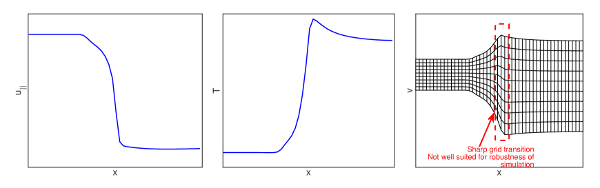
Figure 5.1: Illustration of plasma-shock flow velocity (left), temperature (center), and the corresponding grid quality (right) near the shock front.

For strong shocks, sharp temperature and drift velocity (in terms of $v_{th}$) variations exist near the shock front. These large variations in $v_{th}$ and $\widehat{u}_{||}$ will cause the velocity space grid to be expanded/shifted rapidly both in space and time, resulting in a numerical brittleness. In this study, we address these issues by combining: 1) an empirical temporal limiter, and 2) a spatial smoothing operation, similarly to how we dealt with the monitor function. We note, that neither of these strategies result in a loss of numerical accuracy in principle, as the transformed equations are correct for an arbitrary $v^{*}$ and $\widehat{u}_{||}^{*}$. We elaborate on these strategies next.

In order to limit the velocity grid expansion/contraction and shifting rate in time, we limit the change of updates of $v^{*}$ and $u_{||}^{*}=v^{*}\widehat{u}_{||}^{*}$ by $5\%$ from between time step, i.e.:

$$v_{\alpha}^{*,(p+1)}=\begin{cases}v_{\alpha}^{*,(p)}+\Delta t^{(p)}\dot{v}_{\alpha}^{*,(p+1)}&\textnormal{if}\;\Delta t^{(p)}\frac{\left|\dot{v}_{\alpha}^{*,(p+1)}\right|}{v_{\alpha}^{*,(p)}}\leq 0.05\\ v_{\alpha}^{*,(p)}\left[1+0.05\Delta t\textnormal{sign}\left(\dot{v}_{\alpha}^{*,(p+1)}\right)\right]&\textnormal{otherwise}\end{cases},$$ (5.50)

and

$$u_{||,\alpha}^{*,(p+1)}=\begin{cases}u_{||,\alpha}^{*,(p)}+\Delta t^{(p)}\dot{u}_{||,\alpha}^{*,(p+1)}&\textnormal{if}\;\Delta t^{(p)}\left|\frac{\dot{u}_{||,\alpha}^{*,(p+1)}}{v_{\alpha}^{*,(p)}}\right|\leq 0.05\\ u_{||,\alpha}^{*,(p)}\left[1+0.05\Delta t\textnormal{sign}\left(\dot{u}_{||,\alpha}^{*,(p+1)}\right)\right]&\textnormal{otherwise}\end{cases},$$ (5.51)

where

$$\dot{v}_{\alpha}^{*,(p+1)}=\frac{\left[v_{\alpha}^{*,(p+1)}\right]^{\dagger}-v_{\alpha}^{*,(p)}}{\Delta t^{(p)}},\;\dot{u}_{||,\alpha}^{*,(p+1)}=\frac{\left[u_{||,\alpha}^{*,(p+1)}\right]^{\dagger}-u_{||,\alpha}^{*,(p)}}{\Delta t^{(p)}},$$

and

$$\left[v_{\alpha}^{*,(p+1)}\right]^{\dagger}=\sqrt{\frac{2T_{\alpha}^{(p+1)}}{m_{\alpha}}},\;\left[u_{||,\alpha}^{*,(p+1)}\right]^{\dagger}=u_{||,\alpha}^{(p+1)}+\Delta w_{||,\alpha}^{(p+1)},$$

$$\Delta w_{||,\alpha}^{(p+1)}=\frac{\left\langle\left(v_{||}^{(p)}-u_{||,\alpha}^{(p+1)}\right)\left(\mathbf{v}^{(p)}-\mathbf{u}_{\alpha}^{(p+1)}\right)^{2},f_{\alpha}^{(p+1)}\right\rangle_{v}}{\left\langle\left(\mathbf{v}^{(p)}-\mathbf{u}_{\alpha}^{(p+1)}\right)^{2},f_{\alpha}^{(p+1)}\right\rangle_{v}}.$$

Here $\Delta w_{||}$ is a measure of skewness in the distribution function and is included to better account for non-thermal structures.

To ensure that the profiles of $v^{*}$ and $u_{||}^{*}$ are smooth in space, we employ a Winslow smoother. We solve the following elliptic equation for $\phi$,

$$\left[1-\lambda_{\phi}\partial_{\xi\xi}\right]\phi=\phi^{*}.$$ (5.52)

Here, note that $\phi^{*}$ is the pre-smoothed quantity [$v^{*}$ and $u^{*}$ from Eqs. (5.50) and (5.51)], $\phi$ is the post-smoothed quantity, $\lambda_{\phi}=10^{-2}$ is the empirically determined smoothing coefficient, and that $\widehat{u}_{||}^{*}=u_{||}^{*}/v^{*}$ is computed after smoothing $v^{*}$ and $u_{||}^{*}$. Refer to Fig. 5.2 for an illustration of the effects of post-grid-smoothing operation.

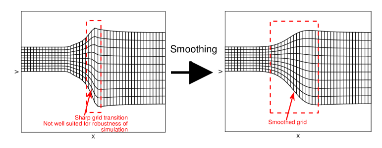
Figure 5.2: Illustration of unsmoothed (left) and smoothed (right) phase-space grid in a plasma-shock problem.

6 Numerical Results

In this section, we demonstrate the conservation, order of accuracy, and computational savings properties of our numerical implementation, with various examples of varying degrees of complexity. For all problems, we normalize the mass, charge, temperature, density, velocity, and time to the proton mass, $m$, proton charge, $e$, reference temperature, $T^{0}$, density, $n^{0}$, characteristic speed, $v^{0}=\sqrt{T^{0}/m}$, and time-scale, $\tau^{0}=\frac{3\sqrt{m}\left(T^{0}\right)^{3/2}}{4\sqrt{\pi}n^{0}\Lambda e^{4}}$, respectively. A constant Coulomb logarithm, $\Lambda=10$, is used everywhere unless otherwise stated. All normalized distribution functions are initialized as Maxwellians, with prescribed moments in $n$, $u_{||}$, and $T$ as:

$$\widetilde{f}_{M}=\frac{n}{\pi^{3/2}}\left(\frac{v^{*}}{v_{th}}\right)^{3}\textnormal{exp}\left[-\frac{\left(v^{*}\widetilde{v}_{||}+u_{||}^{*}-u_{||}\right)^{2}+\left(v^{*}\widetilde{v}_{\perp}\right)^{2}}{v_{th}^{2}}\right].$$ (6.1)

The initial profiles of the normalization speed, $v^{*}(\xi)$, and shift velocity, $u_{||}^{*}\left(\xi\right)$, are found by applying a Winslow smoothing (unless otherwise stated, $\lambda_{\phi}=10^{-2}$), such that high wavenumber components of the initial temperature profile (if present) are smoothed out to prevent large numerical errors stemming from the computation of spatial gradients of $v^{*}$ and $u_{||}^{*}$ in the inertial term. We note that, in this study, we use a discrete quadrature error accounting technique to ensure that discrete Maxwellian moments agree exactly with the prescribed ones [32]. Also, for post-processing purposes the cell-center location of configuration-space is computed from a linear interpolation of cell-face location, $x_{i}=0.5(x_{i+1/2}+x_{i-1/2})$.

The nonlinearly-coupled discrete ion Vlasov-Fokker-Planck and fluid electron equations are solved using an Anderson accelerated fixed-point iterative solver [33] with a nonlinear elimination strategy for the Rosenbluth potentials (similar to Ref. [20]) and similar preconditioning strategies (multi-grid solver and operator-splitting) as discussed in Refs. [20, 34]. Finally, unless otherwise stated, we employ a nonlinear convergence tolerance of $\epsilon_{r}=10^{-3}$.

6.1 Particle-beam relaxation

We test the basic capability of velocity-space grid adaptivity by simulating a particle-beam relaxation in a background plasma. Specifically, we consider a background Aluminum plasma ($m_{Al}=27$ and $q_{Al}=13$ ) with a number density of $n_{Al,0}=1$, temperature of $T_{Al,0}=1$ ($v_{th,Al}=0.272)$ and a drift velocity of $u_{||,Al,0}=0$; and a Deuteron beam ($m_{D}=2$ and $q_{D}=1$) with an initial temperature of $T_{D,0}=0.01$ ($v_{th,D}=0.1$), and a drift velocity of $u_{||,D,0}=30v_{th,Al}$. We choose a velocity-space domain of $\widetilde{v}_{||}\times\widetilde{v}_{\perp}\in\left[-5,5\right]\times\left[0,5\right]$ and a mesh size of $N_{||}\times N_{\perp}=64\times 32$.

We note that, for static grids, modeling of a particle-beam relaxation is notoriously challenging due to the requirements of having to simultaneously resolve the initially cold beam, and also being able to have a large enough velocity-space domain to accommodate the intermediate broad (hot) distribution function. If sufficient resolution is not provided for the beam, important dynamic quantities, such as the velocity-space parallel and perpendicular diffusion rates, cannot be captured accurately.

In Fig. 6.1, we show the evolution of the beam distribution function for different snapshots in time.

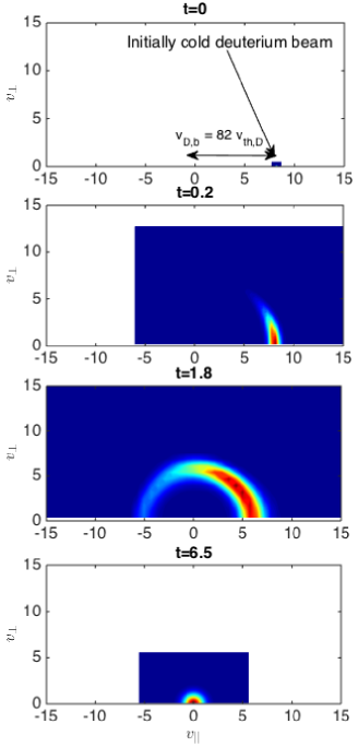
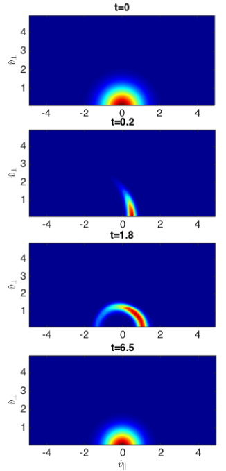
Figure 6.1: Particle-beam relaxation: Evolution of the beam distribution function for various times in the physical (left column) and the transformed coordinates (right column).

As can be seen, the classic isotropization process takes place, followed by the thermalization. It can also be seen that the grid dynamically evolves with the temperature and drift velocities of the distribution function, providing an optimal balance between grid resolution and computational complexity at all times.

Next, we demonstrate the accuracy of the new method by comparing the beam slowing down, as well as the parallel and perpendicular diffusion rates with theory predictions [35],

$$\nu_{s}^{D\backslash Al}=\left(1+m_{D}/m_{Al}\right)\psi\left(x^{D\backslash Al}\right)\nu_{0}^{D\backslash Al},$$

$$\nu_{\perp}^{D\backslash Al}=2\left[\left(1-1/2x^{D\backslash Al}\right)\psi\left(x^{D\backslash Al}\right)+\psi^{\prime}\left(x^{D\backslash Al}\right)\right]\nu_{0}^{D\backslash Al},$$

$$\nu_{||}^{D\backslash Al}=\left[\psi\left(x^{D\backslash Al}\right)/x^{D\backslash Al}\right]\nu_{0}^{D\backslash Al},$$

where

$$\nu_{0}^{D\backslash Al}=\frac{4\pi e_{D}^{2}e_{Al}^{2}\Lambda_{DAl}n_{Al}}{m_{D}^{2}u_{||,D,0}^{3}},\;x^{D\backslash Al}=u_{||,D,0}^{2}/v_{th,Al,0}^{2},\;\psi=\frac{2}{\sqrt{\pi}}\int_{0}^{x}t^{1/2}e^{-t}dt,\;\psi^{\prime}\left(x\right)=\frac{d\psi}{dx}.$$

We time average the simulated quantities to increase numerical accuracy:

$$\left\langle\overline{\nu_{s}^{D\backslash Al}}\right\rangle_{\tau}=\sum_{p=1}^{N_{t}}\left|\frac{u_{||,D}^{(p)}-u_{||,D}^{(p-1)}}{u_{||,D}^{(p)}}\right|/\sum_{p=1}^{N_{t}}\Delta t^{(p)},\;\textnormal{where}\;u_{||,D}^{(p)}=\frac{\left\langle v_{||}^{(p-1)},f_{D}^{(p)}\right\rangle_{v}}{\left\langle 1,f_{D}^{(p)}\right\rangle_{v}}$$

$$\left\langle\overline{\nu_{||}^{D\backslash Al}}\right\rangle_{\tau}=\sum_{p=1}^{N_{t}}\left|\frac{T_{||,D}^{(p)}-T_{||,D}^{(p-1)}}{\left[u_{||,D}^{(p)}\right]^{2}}\right|/\sum_{p=1}^{N_{t}}\Delta t^{(p)},\;\textnormal{where}\;T_{||,D}^{(p)}=\frac{m_{D}\left\langle\left(v_{||}^{(p-1)}-u_{||,D}^{(p)}\right)^{2},f_{D}^{(p)}\right\rangle_{v}}{\left\langle 1,f_{D}^{(p)}\right\rangle_{v}}.$$

$$\left\langle\overline{\nu_{\perp}^{D\backslash Al}}\right\rangle_{\tau}=\sum_{p=1}^{N_{t}}\left|\frac{T_{\perp,D}^{(p)}-T_{\perp,D}^{(p-1)}}{\left[u_{||,D}^{(p)}\right]^{2}}\right|/\sum_{p=1}^{N_{t}}\Delta t^{(p)},\;\textnormal{where}\;T_{\perp,D}^{(p)}=\frac{m_{D}\left\langle\left(v_{\perp}^{(p-1)}\right)^{2},f_{D}^{(p)}\right\rangle_{v}}{2\left\langle 1,f_{D}^{(p)}\right\rangle_{v}}.$$

The results are shown in Fig. 6.2 for various initial Deuteron-beam velocities. Here, $N_{t}$ is the maximum number of time steps chosen based on the averaging, which is performed until

$$\left|T_{\perp,D}\left(t=t_{f}\right)-T_{\perp,D}\left(t=t_{0}\right)\right|/T_{\perp,D}\left(t=t_{0}\right)>0.01.$$

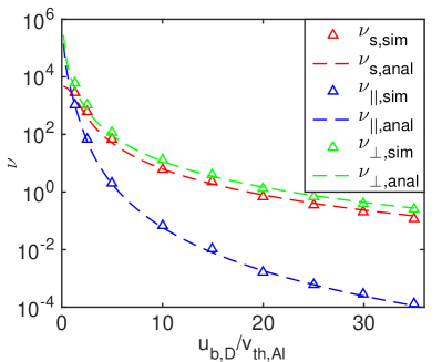
Figure 6.2: Particle beam relaxation: Comparison between numerical (triangles) and theoretical (dashed lines) predictions for a Deuterium-beam slowing down, parallel, and perpendicular diffusion rates on an Aluminum background.

Good agreement is seen across a wide range of beam velocities, demonstrating the accuracy of the proposed grid-adaptivity scheme.

6.2 Two-beam thermal and drift relaxation

Next, we simulate relaxation of two counter-streaming Maxwellians with disparate velocities. The purpose of this simulation is to demonstrate the importance of satisfying the discrete temporal-conservation symmetries arising from the velocity-space grid adaptivity [e.g., Eqs. (5.29) and (5.31)]. We compare the solutions obtained with and without ensuring the symmetries. We consider two Deuteron beams ($q=1$ and $m=2$) with equal number densities, $n=1$, and temperatures, $T=0.01$ ($v_{th}=0.1$), but with disparate initial drift velocities, $u_{||,1}=-100v_{th}$ and $u_{||,2}=100v_{th}$. We choose a velocity-space domain of $\widetilde{v}_{||}\times\widetilde{v}_{\perp}\in\left[-5,5\right]\times\left[0,5\right]$ and a mesh size of $N_{||}\times N_{\perp}=32\times 16$. Through collisions, the two beams will equilibrate to a common drift velocity of $u_{||}=0$ and a temperature of $T=66\frac{2}{3}$; refer to Fig. 6.3.

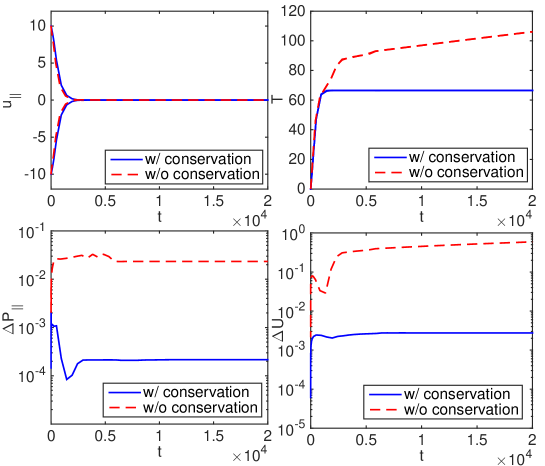
Figure 6.3: Two-beam thermal and drift relaxation: Dynamic relaxation of two species temperature (top left) and drift velocity (top right) with (solid line) and without (dashed line) discrete momentum (bottom left) and energy (bottom right) conservation imposed.

Here,

$$\Delta P_{||}=\left|\frac{\sum_{i}^{N_{\xi}}\sum_{\alpha}^{N_{sp}}J_{\xi,i}^{(p=0)}P_{||,\alpha,i}^{(p=0)}-\sum_{i}^{N_{\xi}}\sum_{\alpha}^{N_{sp}}J_{\xi,i}P_{||,\alpha,i}}{\sum_{i}^{N_{\xi}}\sum_{\alpha}^{N_{sp}}J_{\xi,i}^{(p=0)}P_{||,\alpha,i}^{(p=0)}}\right|$$

is the relative variation of the total momentum of the system and

$$\Delta U=\left|\frac{\sum_{i}^{N_{\xi}}\sum_{\alpha}^{N_{sp}}J_{\xi,i}^{(p=0)}U_{\alpha,i}^{(p=0)}-\sum_{i}^{N_{\xi}}\sum_{\alpha}^{N_{sp}}J_{\xi,i}U_{\alpha,i}}{\sum_{i}^{N_{\xi}}\sum_{\alpha}^{N_{sp}}J_{\xi,i}^{(p=0)}U_{\alpha,i}^{(p=0)}}\right|$$

is the relative variation of the total kinetic energy of the system; $P_{||,\alpha,i}=m_{\alpha}\left\langle v_{||,i},\widetilde{f}_{\alpha,i}\right\rangle_{\delta\widetilde{\mathbf{v}}}$ and $U_{\alpha,i}=m_{\alpha}\left\langle\frac{v_{,i}^{2}}{2},\widetilde{f}_{\alpha,i}\right\rangle_{\delta\widetilde{\mathbf{v}}}$. Also, $i$ is the grid index in the configuration space, and the superscript $p=0$ denotes the initial-time quantities. As can be seen, without the temporal-Vlasov discrete-conservation symmetries, the system numerically heats indefinitely. Thus, a moving-grid strategy is by itself, not sufficient to reduce the computational complexity, as stable asymptotic solutions cannot be achieved in general without a discrete conservation principle.

6.3 1D2V sinusoidal perturbation relaxation with prescribed grid motion

We simulate a relaxation of a sinusoidal perturbation with a prescribed grid motion. The purpose of this simulation is to demonstrate the importance of satisfying the discrete conservation symmetries arising from grid motion in configuration space. Consider a proton-electron plasma ($q_{p}=1$, $q_{e}=-1$, $m_{p}=1$, and $m_{e}=1/1836$) in a periodic domain with initial density, drift velocity, and temperature profiles given by:

$$n_{0}=1+0.5\sin\left(k_{x}x\right),$$

$$u_{||,0}=0.9\sin\left(k_{x}x\right),$$

$$T_{0}=1+0.9\sin\left(k_{x}x\right),$$

where, $x\in[0,L_{x}]$, $L_{x}=10$ is the configuration-space domain size, $k_{x}=2\pi/L_{x}$, and a time-dependent grid given by:

$$x\left(\xi_{i},t\right)=x_{0,i}+0.45\Delta x_{0}\sin\left(\omega_{grid}t\right)\cos\left(k_{x}x_{0,i}\right).$$

Here, $\Delta x_{0}=L_{x}/N_{\xi}$ is the average grid size, $N_{\xi}=24$, $x_{0}=\xi L_{x}$ is the initial grid, $\xi\in\left[0,1\right]$ is the logical grid coordinate, and $\omega_{grid}=4\pi/5$ is the grid oscillation frequency. In the velocity space, we employ the domain $\widetilde{v}_{||}\times\widetilde{v}_{\perp}\in\left[-7,7\right]\times\left[0,7\right]$, and the grid $N_{||}\times N_{\perp}=32\times 16$. In Fig. 6.4, we compare the drift velocity and temperature of the protons at the equilibrium time ($t\sim 50$), with and without enforcing the Vlasov temporal and spatial discrete conservation symmetries [Eqs. (5.29),(5.31),(5.45), and (5.46)].

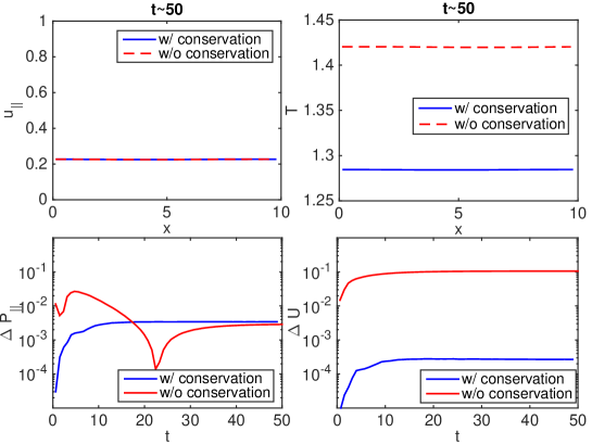
Figure 6.4: 1D2V Sinusoidal perturbation relaxation: Dynamic relaxation of initial drift velocity (top left) and temperature (top right) with (solid) and without (dashed) the Vlasov discrete conservation symmetries, and the associated momentum (bottom left) and energy (bottom right) conservation error as a function of time.

As can be seen, the lack of discrete conservation manifests as numerical heating, underlying the importance of satisfying the respective theorems. In Fig. 6.5, we show the quality of conservation with varying nonlinear-convergence tolerance; and demonstrate that the quality improves with the tighter tolerance.

Figure 6.5: 1D2V Sinusoidal perturbation relaxation: Conservation of mass, momentum, and energy for various nonlinear convergence tolerances.

To demonstrate the second-order temporal convergence of the BDF2 scheme that we employ, we compute the relative difference of the plasma temperature with respect to the reference quantity,

$${\cal E}_{T}^{\Delta t}=\sum_{i=1}^{N_{\xi}}\Delta\xi\frac{\left|T_{i}^{\Delta t,ref}-T_{i}^{\Delta t}\right|}{T_{i}^{\Delta t,ref}}.$$ (6.2)

Here, $T^{\Delta t,ref}$ is the reference temperature obtained using a small time-step size ($\Delta t_{ref}=10^{-3}$) at the final time $t_{max}=0.5$. For all cases, we use a grid size of $N_{\xi}=24$ and $N_{v}=32\times 16$, and a solver nonlinear convergence tolerance of of $\epsilon_{r}=10^{-6}$ (to adequately capture small signals for small $\Delta t$). Fig. 6.6-left shows the expected asymptotic second order accuracy with $\Delta t$ refinement.

A second-order accuracy in velocity-space is demonstrated similarly by computing:

$${\cal E}_{T}^{\Delta\widetilde{v}}=\sum_{i=1}^{N_{\xi}}\Delta\xi\frac{\left|T_{i}^{\Delta\widetilde{v},ref}-T_{i}^{\Delta\widetilde{v}}\right|}{T_{i}^{\Delta\widetilde{v},ref}}.$$ (6.3)

Here, $T^{\Delta\widetilde{v},ref}$ is the reference temperature solution obtained using a reference-grid resolution of $N_{v}^{ref}=512\times 256$. A uniform grid refinement is performed in both velocity-space directions. For all cases, we use $\Delta t=5\times 10^{-2}$ and a final time $t_{max}=0.5$ with $N_{\xi}=24$. Fig. 6.6-center confirms the second-order convergence with $\Delta\widetilde{v}$ refinement.

Finally, to demonstrate a second-order accuracy of the spatial discretization, we use a similar approach and compute

$${\cal E}_{T}^{\Delta\xi}=\sum_{i=1}^{N_{\xi,ref}}\Delta\xi_{ref}\frac{\left|T_{i}^{\Delta\xi,ref}-T_{i}^{\Delta\xi}\right|}{T_{i}^{\Delta\xi,ref}}.$$ (6.4)

Here, $T^{\Delta\xi,ref}$ and $\Delta\xi_{ref}$ are the reference-temperature solution and logical-grid size, respectively, obtained using a reference-grid resolution ($N_{\xi,ref}=768$) with $\Delta t=5\times 10^{-2}$ and $t_{max}=0.5$. To compute the norm in Eq. (6.4), we interpolate the coarse solution onto the reference configuration-space grid (e.g., in $x$) via a $4^{th}$ order spline. For all cases, we use a velocity space grid size of $N_{v}=32\times 16$. Fig. 6.6-right confirms the expected second order of accuracy of our spatial discretization.

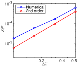
Figure 6.6: 1D2V Sinusoidal perturbation relaxation: Temporal- (left), velocity-space- (center), and spatial- (right) order accuracy of the proposed scheme. Second-order accuracy is confirmed in all cases.

6.4 1D2V Mach 5 Standing Shock

We simulate a Mach-5 standing shock problem. The purpose of this simulation is to demonstrate that the proposed phase-space grid adaptivity and associated discrete-conservation strategy can reproduce published results in the literature [16, 36]. We obtain the hydrodynamic jump conditions from the Hugoniot relationship:

$$\frac{P_{1}}{P_{0}}=\frac{2\gamma M^{2}-(\gamma-1)}{\gamma+1},$$ (6.5)

$$\frac{\rho_{1}}{\rho_{0}}=\frac{u_{0}}{u_{1}}=\frac{M^{2}\left(\gamma+1\right)}{M^{2}\left(\gamma-1\right)+2}.$$ (6.6)

Here, the subscript $0$ denotes the upstream (un-shocked) region and the subscript $1$ denotes the downstream (shocked) region. Combining these equations gives:

$$\frac{u_{0}}{u_{1}}=\frac{\left(\gamma-1\right)P_{0}+\left(\gamma+1\right)P_{1}}{\left(\gamma+1\right)P_{0}+\left(\gamma-1\right)P_{1}}.$$ (6.7)

Here, $\gamma$ is the specific heat ratio ($\gamma=5/3$ for fully ionized plasmas), $P$ is the total plasma pressure (i.e., $P=P_{i}+P_{e}$), $\rho=\sum_{\alpha=1}^{N_{s}}m_{\alpha}n_{\alpha}$ is the total mass density, and $u=\sum_{\alpha=1}^{N_{s}}m_{\alpha}n_{\alpha}u_{\alpha}/\sum_{\alpha=1}^{N_{s}}m_{\alpha}n_{\alpha}$ is the mass averaged drift velocity of the respective regions. The upstream velocity can be expressed as

$$u_{0}=Mc_{0},$$ (6.8)

where $c_{0}$ is the upstream sound speed,

$$c_{0}=\sqrt{\gamma\frac{P_{0}}{\rho_{0}}}.$$ (6.9)

Employing the downstream conditions of $\rho_{1}=mn_{1}=1,$ $n_{1}=1$, $m_{1}=1$, $P_{1}=P_{1,i}+P_{1,e}=2P_{1,i}=2n_{1,i}T_{1,i}=2$, $T_{1,i}=1$, and $M=5$ gives for the upstream conditions $\rho_{0}=mn_{0}=0.28$, $P_{0}=0.1290$, and $T_{0}=0.1152$ . Then, $c_{0}=0.6197$, $u_{0}=Mc_{0}=3.0984$, and $u_{1}=0.8676$. We note that, for this case and for comparison purposes with Ref. [16], we employ a variable Coulomb logarithm for both ion-ion and ion-electron collisions [35], with $T^{0}=10$ keV and $n^{0}=10^{22}$ cm^-3.

To stress the computational savings afforded by the adaptivity strategy, we consider a computational domain of $x\times\widetilde{v}_{||}\times\widetilde{v}_{\perp}\in\left[0,200\right]\times\left[-6,6\right]\times\left[0,6\right]$, with a grid of $N_{\xi}=48$, $N_{v}=64\times 32$. For comparison, Ref. [16] used $N_{x}=192$, $N_{v}=128\times 64$. The solution is initialized with a smoothed hyperbolic tangent with the following profiles:

$$n=a_{n}\textnormal{tanh}\left[\mu\left(x-100\right)\right]+b_{n},\;u=a_{u}\textnormal{tanh}\left[\mu\left(x-100\right)\right]+b_{u},\;T=a_{T}\textnormal{tanh}\left[\mu\left(x-100\right)\right]+b_{T}$$

where $a_{n}=0.36$, $b_{n}=0.64$, $a_{u}=-1.1154$, $b_{u}=1.983$, $a_{T}=0.4424$, $b_{T}=0.5576$, and $\mu=0.05$.

In the configuration space, we consider the following in- and out-flow boundary conditions for the ion distribution functions:

$$f_{B}\left(v_{||},v_{\perp}\right)=\begin{cases}f_{M}\left(n_{B},u_{B},T_{B}\right)&\textnormal{if}\;\widehat{l}_{B}v_{||}\leq 0\\ f_{C}&\textnormal{otherwise}\end{cases}.$$ (6.10)

Here, $n_{B}$, $u_{B}$, and $T_{B}$ are the moments defined by the Hugoniot conditions at the boundary, $\widehat{l}_{B}$ is the $x$-component of the boundary surface normal vector ($\pm 1$ in 1D), and $f_{C}$ is the distribution function defined in the computational cell inside the domain, adjacent to the boundary. For the fluid-electron temperature, we use the Dirichlet boundary conditions to impose the Hugoniot asymptotic jump.

The simulation was run to $t_{max}=250$ until transient structures had equilibrated.

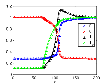
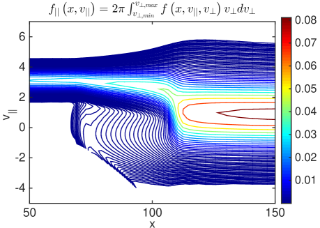
Figure 6.7: Mach 5 steady-state shock: Left–The triangle markers are from our simulation, while the solid lines are from Ref. [16] for a similar setup. We note that in the plot, the drift velocity, $u$, is normalized to the upstream value. Right– The perpendicular-velocity-integrated distribution function of the protons.

Excellent agreement is found with respect to the reference solution [16]; refer to Fig. 6.7-left. Also seen in Fig. 6.7-right is a highly non-Maxwellian feature in the distribution function, similar to those observed in Fig. 4.8 of Ref. [16]. In Fig. 6.8, we also show the evolution of the configuration-space grids at different times to demonstrate the MMPDE strategy based on the inverse-gradient-length scale monitor function in Eq. (4.2).

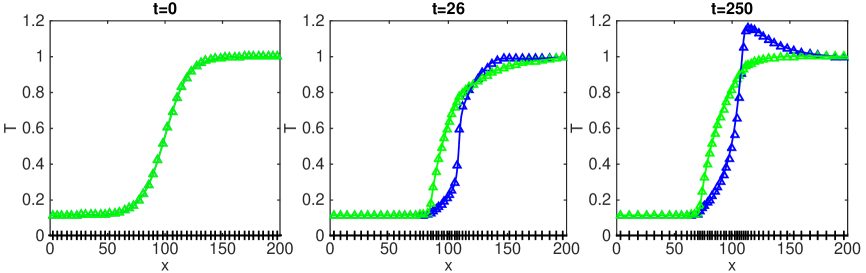
Figure 6.8: Mach 5 steady-state shock: Proton (blue) and electron (green) temperatures at initial (left), intermediate (center), and steady-state (right) times. The solid lines denote the solution obtained by a uniform-static mesh in configuration space ($N_{\xi}=192$) while the triangle markers denote the solution obtained with a coarse grid and adaptivity. As can be seen, the configuration-space grid (+) adapts to the variation in the gradients of temperature, as well as density and drift velocity (not shown).

As can be seen, the configuration-space grid tracks evolving features near sharp gradients 1) without changing the total number of unknowns as other adaptivity strategies do (e.g., AMR) and 2) without significantly compromising the quality of the solution.

Finally, to stress once again the importance of enforcing discrete conservation, we compare the ion temperature of the simulations with and without the Vlasov temporal- and spatial-conservation symmetries enforced; refer to Fig. 6.9.

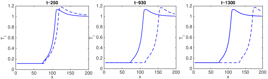
Figure 6.9: Mach 5 steady-state shock: Comparison of proton temperatures obtained with (solid) and without (dashed) enforcing the Vlasov discrete conservation symmetries.

As can be seen, without discrete conservation, the shock front drifts indefinitely, resulting in ${\cal O}\left(1\right)$ error. In multiple time-scale simulations, such subtle features can manifest as a departure of the solution from the asymptotic slow manifold (e.g., hydrodynamic limit), polluting the numerical results and making their physical interpretation difficult.

7 Conclusion

In this study, we have demonstrated, for the first time, an approach that is fully conservative and adaptive in the phase space $\left(x,\mathbf{v}\right)$ for the multi-species, 1D2V VFP ion plasma equations with fluid electrons. The approach features exact (in practice, up to a nonlinear tolerance) mass, momentum, and energy conservation. Our approach analytically adapts the velocity-space mesh for each species by normalizing the velocity space to each species’ reference speed, $v^{*}$, and shifting by a translation velocity, $u_{||}^{*}$ (i.e., we consider multiple velocity-space grids), and allows for an arbitrary variation (in practice, to acceptable level of truncation error) in $v_{th}$ and $u_{||}$. In configuration-space, we transform the VFP-ion and fluid-electron equations on a logically Cartesian grid, and the Jacobian of transformation is evolved using an MMPDE formalism. The analytical formulation allows us to expose the continuum-conservation symmetries in the inertial terms arising from the coordinate transformation, which are then enforced discretely via the use of discrete-nonlinear constraint functions, as proposed in earlier studies [30, 20, 21, 16]. We have shown the importance of enforcing the discrete conservation and the adverse effects of not doing so for several test cases. We close by noting that the methodology developed in this study has been extended to a spherical geometry with an imploding boundary to study ICF capsule implosion [37]. This work will be documented in a follow-on manuscript.

Appendix A Derivation of Vlasov-Fokker-Planck Equation in the Transformed Coordinate System

Beginning with the 1D Vlasov equation in the original coordinates, $\left(x,\mathbf{v},t\right)$,

$$\left.\frac{\partial f}{\partial t}\right|_{x,\mathbf{v}}+v_{||}\left.\frac{\partial f}{\partial x}\right|_{\mathbf{v},t}+\frac{q}{m}E_{||}\left.\frac{\partial f}{\partial v_{||}}\right|_{x,t}=0,$$ (A.1)

and introducing the coordinates, $\left(\xi,\mathbf{\widetilde{v}},t\right)$, we expand each term as follows:

$$\left.\frac{\partial f}{\partial t}\right|_{x,\mathbf{v}}=\left.\frac{\partial f}{\partial t}\right|_{\xi,\mathbf{v}}-\left.\frac{\partial f}{\partial\xi}\right|_{\mathbf{v},t}J_{\xi}^{-1}\dot{x}$$

$$=\left.\frac{\partial f}{\partial t}\right|_{\xi,\mathbf{\widetilde{v}}}+\left.\frac{\partial f}{\partial\widetilde{\mathbf{v}}}\right|_{\xi,t}\cdot\left(\frac{\partial\widetilde{\mathbf{v}}}{\partial v^{*}}\frac{\partial v^{*}}{\partial t}+\frac{\partial\widetilde{\mathbf{v}}}{\partial\widehat{\mathbf{u}}^{*}}\cdot\frac{\partial\widehat{\mathbf{u}}^{*}}{\partial t}\right)-\left[\left.\frac{\partial f}{\partial\xi}\right|_{\widetilde{\mathbf{v}},t}+\left.\frac{\partial f}{\partial\widetilde{\mathbf{v}}}\right|_{\xi,t}\cdot\left(\frac{\partial\widetilde{\mathbf{v}}}{\partial v^{*}}\frac{\partial v^{*}}{\partial\xi}+\frac{\partial\widetilde{\mathbf{v}}}{\partial\widehat{\mathbf{u}}^{*}}\cdot\frac{\partial\widehat{\mathbf{u}}^{*}}{\partial\xi}\right)\right]J_{\xi}^{-1}\dot{x},$$ (A.2)

$$v_{||}\left.\frac{\partial f}{\partial x}\right|_{\mathbf{v},t}=v^{*}\left(\widetilde{v}_{||}+\widehat{u}_{||}^{*}\right)\left.\frac{\partial f}{\partial\xi}\right|_{\mathbf{v},t}J^{-1}=v^{*}\left(\widetilde{v}_{||}+\widehat{u}_{||}^{*}\right)\left[\left.\frac{\partial f}{\partial\xi}\right|_{\widetilde{\mathbf{v}},t}+\left.\frac{\partial f}{\partial\widetilde{\mathbf{v}}}\right|_{\xi,t}\cdot\left(\frac{\partial\widetilde{\mathbf{v}}}{\partial v^{*}}\frac{\partial v^{*}}{\partial\xi}+\frac{\partial\widetilde{\mathbf{v}}}{\partial\widehat{\mathbf{u}}^{*}}\cdot\frac{\partial\widehat{\mathbf{u}}^{*}}{\partial\xi}\right)\right]J_{\xi}^{-1},$$ (A.3)

and

$$\frac{q}{m}E_{||}\left.\frac{\partial f}{\partial v_{||}}\right|_{x,t}=\frac{q}{m}\frac{E_{||}}{v^{*}}\left.\frac{\partial f}{\partial\widetilde{v}_{||}}\right|_{\xi,t},$$ (A.4)

where,

$$J_{\xi}^{-1}=\frac{\partial\xi}{\partial x},\;\dot{x}=\frac{\partial x}{\partial t},\frac{\partial\widetilde{\mathbf{v}}}{\partial v^{*}}=-\frac{\widetilde{\mathbf{v}}+\widehat{\mathbf{u}}^{*}}{v^{*}},\;\frac{\partial\widetilde{\mathbf{v}}}{\partial\mathbf{\widehat{u}}^{*}}=-\stackrel{{\scriptstyle\leftrightarrow}}{{\mathsfsl{I}}},\;\textnormal{and}\;\widehat{\mathbf{u}}^{*}=\widehat{u}_{||}^{*}\mathbf{e}_{||}.$$

Assembling the terms, we obtain:

$$\left.\frac{\partial f}{\partial t}\right|_{\xi,\mathbf{\widetilde{v}}}-\left.\frac{\partial f}{\partial\widetilde{\mathbf{v}}}\right|\cdot\left(\frac{\widetilde{\mathbf{v}}+\widehat{u}_{||}^{*}\mathbf{e}_{||}}{v^{*}}\frac{\partial v^{*}}{\partial t}+\frac{\partial\widehat{u}_{||}^{*}}{\partial t}\mathbf{e}_{||}\right)-\left[\left.\frac{\partial f}{\partial\xi}\right|_{\widetilde{\mathbf{v}},t}-\left.\frac{\partial f}{\partial\widetilde{\mathbf{v}}}\right|_{\xi,t}\cdot\left(\frac{\widetilde{\mathbf{v}}+\widehat{u}_{||}^{*}\mathbf{e}_{||}}{v^{*}}\frac{\partial v^{*}}{\partial\xi}+\frac{\partial\widehat{u}_{||}^{*}}{\partial\xi}\mathbf{e}_{||}\right)\right]J_{\xi}^{-1}\dot{x},$$

$$+v^{*}\left(\widetilde{v}_{||}+\widehat{u}_{||}^{*}\right)\left[\left.\frac{\partial f}{\partial\xi}\right|_{\widetilde{\mathbf{v}},t}-\left.\frac{\partial f}{\partial\widetilde{\mathbf{v}}}\right|_{\xi,t}\cdot\left(\frac{\widetilde{\mathbf{v}}+\widehat{u}_{||}^{*}\mathbf{e}_{||}}{v^{*}}\frac{\partial v^{*}}{\partial\xi}+\frac{\partial\widehat{u}_{||}^{*}}{\partial\xi}\mathbf{e}_{||}\right)\right]J_{\xi}^{-1}+\frac{q}{m}\frac{E_{||}}{v^{*}}\left.\frac{\partial f}{\partial\widetilde{v}_{||}}\right|_{\xi,t}=0.$$ (A.5)

Noting that $f=\frac{\widetilde{f}}{\left(v^{*}\right)^{3}}$,

$$\left.\frac{\partial f}{\partial t}\right|_{\xi,\widetilde{\mathbf{v}}}=\frac{1}{\left(v^{*}\right)^{3}}\left.\frac{\partial\widetilde{f}}{\partial t}\right|_{\xi,\widetilde{\mathbf{v}}}-\frac{3\widetilde{f}}{\left(v^{*}\right)^{4}}\frac{\partial v^{*}}{\partial t},$$

$$\left.\frac{\partial f}{\partial\xi}\right|_{\widetilde{\mathbf{v}},t}=\frac{1}{\left(v^{*}\right)^{3}}\left.\frac{\partial\widetilde{f}}{\partial\xi}\right|_{\widetilde{\mathbf{v}},t}-\frac{3\widetilde{f}}{\left(v^{*}\right)^{4}}\frac{\partial v^{*}}{\partial\xi},$$

and multiplying Eq. (A.5) by $\left(v^{*}\right)^{3}J_{\xi}$, one obtains,

$$J_{\xi}\left.\frac{\partial\widetilde{f}}{\partial t}\right|_{\xi,\mathbf{\widetilde{v}}}-J_{\xi}\frac{3\widetilde{f}}{v^{*}}\frac{\partial v^{*}}{\partial t}-J_{\xi}\left.\frac{\partial\widetilde{f}}{\partial\widetilde{\mathbf{v}}}\right|\cdot\left(\frac{\widetilde{\mathbf{v}}+\widehat{u}_{||}^{*}\mathbf{e}_{||}}{v^{*}}\frac{\partial v^{*}}{\partial t}+\frac{\partial\widehat{u}_{||}^{*}}{\partial t}\mathbf{e}_{||}\right)$$

$$-\left[\left.\frac{\partial\widetilde{f}}{\partial\xi}\right|_{\widetilde{\mathbf{v}},t}-\frac{3\widetilde{f}}{v^{*}}\frac{\partial v^{*}}{\partial\xi}-\left.\frac{\partial\widetilde{f}}{\partial\widetilde{\mathbf{v}}}\right|_{\xi,t}\cdot\left(\frac{\widetilde{\mathbf{v}}+\widehat{u}_{||}^{*}\mathbf{e}_{||}}{v^{*}}\frac{\partial v^{*}}{\partial\xi}+\frac{\partial\widehat{u}_{||}^{*}}{\partial\xi}\mathbf{e}_{||}\right)\right]\dot{x}$$

$$+v^{*}\left(\widetilde{v}_{||}+\widehat{u}_{||}^{*}\right)\left[\left.\frac{\partial\widetilde{f}}{\partial\xi}\right|_{\widetilde{\mathbf{v}},t}-\frac{3\widetilde{f}}{v^{*}}\frac{\partial v^{*}}{\partial\xi}-\left.\frac{\partial\widetilde{f}}{\partial\widetilde{\mathbf{v}}}\right|_{\xi,t}\cdot\left(\frac{\widetilde{\mathbf{v}}+\widehat{u}_{||}^{*}\mathbf{e}_{||}}{v^{*}}\frac{\partial v^{*}}{\partial\xi}+\frac{\partial\widehat{u}_{||}^{*}}{\partial\xi}\mathbf{e}_{||}\right)\right]+J_{\xi}\frac{q}{m}\frac{E}{v^{*}}\left.\frac{\partial\widetilde{f}}{\partial\widetilde{v}_{||}}\right|_{\xi,t}=0.$$ (A.6)

Recognizing the following chain-rules,

$$\frac{\partial}{\partial\mathbf{\widetilde{v}}}\cdot\left\{\left(\frac{\widetilde{\mathbf{v}}+\widehat{u}_{||}^{*}\mathbf{e}_{||}}{v^{*}}\frac{\partial v^{*}}{\partial t}+\frac{\partial\widehat{u}_{||}^{*}}{\partial t}\mathbf{e}_{||}\right)\widetilde{f}\right\}_{\xi,t}=\frac{3\widetilde{f}}{v^{*}}\frac{\partial v^{*}}{\partial t}+\left.\frac{\partial\widetilde{f}}{\partial\widetilde{\mathbf{v}}}\right|_{\xi,t}\cdot\left(\frac{\widetilde{\mathbf{v}}+\widehat{u}_{||}^{*}\mathbf{e}_{||}}{v^{*}}\frac{\partial v^{*}}{\partial t}+\frac{\partial\widehat{u}_{||}^{*}}{\partial t}\mathbf{e}_{||}\right),$$

$$\frac{\partial}{\partial\mathbf{\widetilde{v}}}\cdot\left\{\left[v^{*}\left(\widetilde{v}_{||}+\widehat{u}_{||}^{*}\right)-\dot{x}\right]\left(\frac{\widetilde{\mathbf{v}}+\widehat{u}_{||}^{*}\mathbf{e}_{||}}{v^{*}}\frac{\partial v^{*}}{\partial\xi}+\frac{\partial\widehat{u}_{||}^{*}}{\partial\xi}\mathbf{e}_{||}\right)\widetilde{f}\right\}_{\xi,t}=$$

$$3\widetilde{f}\left\{\frac{\left[v^{*}\left(\widetilde{v}_{||}+\widehat{u}_{||}^{*}\right)-\dot{x}\right]}{v^{*}}\frac{\partial v^{*}}{\partial\xi}+\left[\frac{\widetilde{v}_{||}+\widehat{u}_{||}^{*}}{v^{*}}\frac{\partial v^{*}}{\partial\xi}+\frac{\partial\widehat{u}_{||}^{*}}{\partial\xi}\right]v^{*}\right\}$$

$$+\left.\frac{\partial\widetilde{f}}{\partial\widetilde{\mathbf{v}}}\right|_{\xi,t}\cdot\left\{\left[v^{*}\left(\widetilde{v}_{||}+\widehat{u}_{||}^{*}\right)-\dot{x}\right]\left(\frac{\widetilde{\mathbf{v}}+\widehat{u}_{||}^{*}\mathbf{e}_{||}}{v^{*}}\frac{\partial v^{*}}{\partial\xi}+\frac{\partial\widehat{u}_{||}^{*}}{\partial\xi}\mathbf{e}_{||}\right)\right\},$$

$$\left.\frac{\partial}{\partial t}\left(J_{\xi}\widetilde{f}\right)\right|_{\xi,\widetilde{\mathbf{v}}}=J_{\xi}\left.\frac{\partial\widetilde{f}}{\partial t}\right|_{\xi,\widetilde{\mathbf{v}}}+\widetilde{f}\frac{\partial\dot{x}}{\partial\xi},$$

$$\left.\frac{\partial}{\partial\xi}\left(\dot{x}\widetilde{f}\right)\right|_{\widetilde{\mathbf{v}},t}=\dot{x}\left.\frac{\partial\widetilde{f}}{\partial\xi}\right|_{\widetilde{\mathbf{v}},t}+\widetilde{f}\frac{\partial\dot{x}}{\partial\xi},$$

$$\frac{\partial}{\partial\xi}\left[v_{||}^{*}\left(\widetilde{v}_{||}+\widehat{u}_{||}^{*}\right)\widetilde{f}\right]_{\widetilde{\mathbf{v}},t}=v^{*}\left(\widetilde{v}_{||}+\widehat{u}_{||}^{*}\right)\left.\frac{\partial\widetilde{f}}{\partial\xi}\right|_{\widetilde{\mathbf{v}},t}+\widetilde{f}v^{*}\left(\frac{\widetilde{v}_{||}+\widehat{u}_{||}^{*}}{v^{*}}\frac{\partial v^{*}}{\partial\xi}+\frac{\partial\widehat{u}_{||}^{*}}{\partial\xi}\right),$$

$$\frac{1}{v^{*}}\frac{\partial}{\partial t}\left[v^{*}\left(\mathbf{\widetilde{v}}+\widehat{u}_{||}^{*}\mathbf{e}_{||}\right)\right]=\frac{\widetilde{\mathbf{v}}+\widehat{u}_{||}^{*}\mathbf{e}_{||}}{v^{*}}\frac{\partial v^{*}}{\partial t}+\frac{\partial\widehat{u}_{||}^{*}}{\partial t}\mathbf{e}_{||},$$

$$\frac{1}{v^{*}}\frac{\partial}{\partial\xi}\left[v^{*}\left(\mathbf{\widetilde{v}}+\widehat{u}_{||}^{*}\mathbf{e}_{||}\right)\right]=\frac{\widetilde{\mathbf{v}}+\widehat{u}_{||}^{*}\mathbf{e}_{||}}{v^{*}}\frac{\partial v^{*}}{\partial\xi}+\frac{\partial\widehat{u}_{||}^{*}}{\partial\xi}\mathbf{e}_{||}.$$

and substituting these results into the original Vlasov-Fokker-Planck equation, Eq. (2.6), there results the following transformed equation for $\widetilde{f}_{\alpha}\left(\xi,\widetilde{\mathbf{v}},t\right)$,

$$\left.\frac{\partial\left(J_{\xi}\widetilde{f}_{\alpha}\right)}{\partial t}\right|_{\xi,\widetilde{\mathbf{v}}}+\frac{\partial}{\partial\xi}\left[\left(v_{\alpha}^{*}\left[\widetilde{v}_{||}+\widehat{u}_{||,\alpha}^{*}\right]-\dot{x}\right)\widetilde{f}_{\alpha}\right]_{\widetilde{\mathbf{v}},t}-\frac{J_{\xi}}{v_{\alpha}^{*}}\frac{\partial}{\partial\widetilde{\mathbf{v}}}\cdot\left[\frac{\partial}{\partial t}\left(v_{\alpha}^{*}\left[\mathbf{\widetilde{v}}+\widehat{u}_{||,\alpha}^{*}\mathbf{e}_{||}\right]\right)\widetilde{f}_{\alpha}\right]_{\xi,t}$$

$$-\frac{1}{v_{\alpha}^{*}}\frac{\partial}{\partial\widetilde{\mathbf{v}}}\cdot\left[\frac{\partial}{\partial\xi}\left(v_{\alpha}^{*}\left[\mathbf{\widetilde{v}}+\widehat{u}_{||,\alpha}^{*}\mathbf{e}_{||}\right]\right)\left(v_{\alpha}^{*}\left[\widetilde{v}_{||}+\widehat{u}_{||,\alpha}^{*}\right]-\dot{x}\right)\widetilde{f}_{\alpha}\right]_{\xi,t}+J_{\xi}\frac{q_{\alpha}}{m_{\alpha}}\frac{E_{||}}{v_{\alpha}^{*}}\left.\frac{\partial\widetilde{f}_{\alpha}}{\partial\widetilde{v}_{||}}\right|_{\xi,t}=J_{\xi}\left[\sum_{\beta}\widetilde{C}_{\alpha\beta}+\widetilde{C}_{\alpha e}\right],$$ (A.7)

where we have used the definition of the normalized collision operator, $\widetilde{C}_{\alpha\beta}=\left(v_{\alpha}^{*}\right)^{3}C_{\alpha\beta}$ (for further details, we refer the readers to Ref. [21]).

References

- [1] M. N. Rosenbluth, W. M. Macdonald, and D. L. Judd, “Fokker-Planck equation for an inverse-square force,” Phys. Rev., vol. 107, no. 1, pp. 1–6, 1957.
- [2] A. A. Arsen’ev and O. E. Buryac, “On the connection between a solution of the Boltzmann equation and a solution of the Landau-Fokker-Planck equation,” USSR Comput. Maths math. Phys., vol. 17, pp. 241–246, 1991.
- [3] L. Desvillettes, “On asymptotics of the Boltzmann equation when the collisions become grazing,” Trans. Theory and Stat. Phys., vol. 21, no. 3, pp. 259–276, 1992.
- [4] P. Degond and B. Lucquin-Desreux, “The Fokker-Planck asymptotics of the Boltzmann collision operator in the Coulomb case,” Math. Models Meth. Appl. Sci., vol. 2, no. 2, pp. 167–182, 1992.
- [5] T. Goudon, “On Boltzmann equations and Fokker-Planck asymptotics: Influence of grazing collisions,” J. Stat. Phys., vol. 89, no. 3/4, pp. 751–776, 1997.
- [6] L. D. Landau, “The kinetic equation in the case of Coulomb interaction,” Phys. Zs. Sov. Union, vol. 10, pp. 154–164, 1936.
- [7] O. Larroche, “An efficient explicit numerical scheme for diffusion-type equations with a highly inhomogeneous and highly anisotropic diffusion tensor,” J. Comput. Phys., vol. 223, pp. 436–450, 2007.
- [8] O. Larroche, “Kinetic simulations of fuel ion transport in ICF target implosions,” Eur. Phys. J. D, vol. 27, pp. 131–146, 2003.
- [9] D. Jarema, H. J. Bungartz, T. Görler, F. Jenko, T. Neckel, and D. Told, “Block-structured grids for eulerian gyro kinetic simulations,” Comput. Phys. Commun., vol. 198, pp. 105–117, 2016.
- [10] B. E. Peigney, O. Larroche, and V. Tikhonchuk, “Fokker-Planck kinetic modeling of supra thermal -particles in a fusion plasma,” J. Comput. Phys., vol. 278, pp. 416–444, 2014.
- [11] M. Gutnic, M. Haefele, I. Paun, and E. Sonnendrüker, “Vlasov simulations on an adaptive phase-space grid,” Comp. Phys. Comm., vol. 164, pp. 214–219, 2004.
- [12] M. Gutnic, M. Haefele, and E. Sonnendrüker, “Moments conservation in adaptive Vlasov solver,” Nuc. Instr. Meth. in Phys. Research A, vol. 558, pp. 159–162, 2006.
- [13] V. Kolobov, R. Arslanbekov, and D. Levko, “Boltzmann-fokker-planck kinetic solver with adaptive mesh in phase space,” arXiv:1810.09049, 2018.
- [14] O. Larroche, “Ion Fokker-Planck simulation of D-3He gas target implosions,” Phys. Plasmas, vol. 19, p. 122706, 2012.
- [15] A. Inglebert, B. Canaud, and O. Larroche, “Species separation and modification of neutron diagnostics in inertial-confinement fusion,” Euro. Phys. Lett., vol. 107, p. 65003, 2014.
- [16] W. T. Taitano, L. Chacón, and A. N. Simakov, “An adaptive, implicit, conservative 1D-2V multi-species Vlasov-Fokker-Planck multiscale solver in planar geometry,” J. Comput. Phys., vol. 365, pp. 173–205, 2018.
- [17] W. Huang, Y. Ren, and R. D. Russell, “Moving mesh methods based on moving mesh partial differential equations,” J. Comput. Phys., vol. 113, no. 2, pp. 279–290, 1994.
- [18] W. Huang, Y. Ren, and R. D. Russell, “Moving mesh partial differential equations (MMPDEs) based on the equidistribution principle,” SIAM J. Numer. Anal., vol. 31, no. 3, pp. 709–730, 1994.
- [19] C. J. Budd, W. Huang, and R. D. Russell, “Adaptivity with moving grids,” Acta Numerica, vol. 18, pp. 111–241, 2009.
- [20] W. T. Taitano, L. Chacón, A. N. Simakov, and K. Molvig, “A mass, momentum, and energy conserving, fully implicit, scalable algorithm for the multi-dimensional, multi-species Rosenbluth-Fokker-Planck equation,” J. Comput. Phys., vol. 297, pp. 357–380, 2015.
- [21] W. T. Taitano, L. Chacón, and A. N. Simakov, “An adaptive, conservative 0D-2V multispecies Rosenbluth-Fokker-Planck solver for arbitrarily disparate mass and temperature regimes,” J. Comput. Phys., vol. 318, pp. 391–420, 2016.
- [22] S. I. Braginskii, “Transport processes in a plasma,” in Reviews of Plasma Physics (M. A. Leontovich, ed.), vol. 1, pp. 205–311, New York: Consultants Bureau, 1965.
- [23] A. N. Simakov and K. Molvig, “Electron transport in a collisional plasma with multiple ion species,” Phys. Plasmas, vol. 21, p. 024503, 2014.
- [24] R. D. Hazeltine and J. D. Meiss, Plasma Confinement. Redwood City, CA: Addison-Wesly Publishing Company, 1991.
- [25] S. Li, L. Petzold, and Y. Ren, “Stability of moving mesh systems of partial differential equations,” SIAM J. Sci. Comput., vol. 20, no. 2, pp. 719–738, 1998.
- [26] G. D. Byrne and A. C. Hindmarsh, “A polyalgorithm for the numerical solution of ordinary differential equations,” ACM Transactions on Mathematical Software, vol. 1, no. 1, pp. 71–96, 1975.
- [27] P. H. Gaskell and A. K. C. Lau, “Curvature-compensated convective transport: SMART, a new boundedness-preserving transport algorithm,” International Journal for Numerical Methods in Fluids, vol. 8, pp. 617–641, 1988.
- [28] E. J. D. Toit, M. R. O’Brien, and R. G. L. Vann, “Positivity-preserving scheme for two-dimensional advection-diffusion equations including mixed derivatives,” Comp. Phys. Comm., vol. 228, pp. 61–68, 2018.
- [29] W. T. Taitano, L. Chacón, A. N. Simakov, and K. Molvig, “A mass, momentum, and energy conserving, fully implicit, scalable algorithm for the multi-dimensional, multi-species rosenbluth-fokker-planck equation,” J. Comput. Phys., vol. 297, pp. 357–380, 2015.
- [30] W. T. Taitano and L. Chacón, “Charge-and-energy conserving moment-based accelerator for a multi-species Vlasov-Fokker-Planck-Ampère system, part I: Collisionless aspects,” J. Comput. Phys., vol. 284, pp. 718–736, 2015.
- [31] A. Winslow, “Numerical solution of the quasi-linear Poisson equation in a nonuniform triangle mesh,” J. Comput. Phys., vol. 1, p. 149, 1967.
- [32] W. T. Taitano, L. Chacón, and A. N. Simakov, “An equilibrium-preserving discretization for the nonlinear Fokker-Planck operator in arbitrary multi-dimensional geometry,” J. Comput. Phys., vol. 339, pp. 453–460, 2017.
- [33] D. G. Anderson, “Iterative procedures for nonlinear integral equations,” J. Assoc. Comput. Mach., vol. 12, pp. 547 – 560, 1965.
- [34] M. Gasteiger, L. Einkemmer, A. Ostermann, and D. Tskhakaya, “Alternating direction implicit type preconditioners for the steady state inhomogeneous Vlasov equation,” J. Plasma Physics., vol. 83, p. 705830107, 2017.
- [35] J. D. Huba, NRL Plasma Formulary. NRL/PU/6790-98-358, Washington, DC: Naval Research Laboratory, 1998.
- [36] F. Vidal, J. P. Matte, M. Casanova, and O. Larroche, “Ion kinetic simulations of the formation and propagation of a planar collisional shock wave in a plasma,” Phys. Plasmas, vol. 5, p. 3182, 1993.
- [37] W. T. Taitano, A. N. Simakov, L. Chacón, and B. Keenan, “Yield degradation in inertial-confinement-fusion implosions due to shock-driven kinetic fuel-species stratification and viscous heating,” Phys. Plasmas, vol. 25, p. 056310, 2018.