On the location of roots of the independence polynomial of bounded degree graphs

Abstract.

In [PR19] Peters and Regts confirmed a conjecture by Sokal [Sok01] by showing that for every $\Delta\in\mathbb{Z}_{\geq 3}$ there exists a complex neighborhood of the interval $\left[0,\frac{\left(\Delta-1\right)^{\Delta-1}}{\left(\Delta-2\right)^{\Delta}}\right)$ on which the independence polynomial is nonzero for all graphs of maximum degree $\Delta$. Furthermore, they gave an explicit neighborhood $U_{\Delta}$ containing this interval on which the independence polynomial is nonzero for all finite rooted Cayley trees with branching number $\Delta$. The question remained whether $U_{\Delta}$ would be zero-free for the independence polynomial of all graphs of maximum degree $\Delta$. In this paper it is shown that this is not the case.

1. Introduction

Let $G=(V,E)$ denote a simple graph. A subset of vertices $I\subseteq V$ is called independent if no two vertices $v_{1},v_{2}\in I$ are connected by an edge in $G$. We define the independence polynomial $Z_{G}$ as

$$Z_{G}(\lambda)=\sum_{\begin{subarray}{c}I\subseteq V\\ \text{independent}\end{subarray}}\lambda^{|I|}.$$ (1)

In statistical physics the independence polynomial occurs as the partition function of the hard-core model.

For any $\Delta\in\mathbb{Z}_{\geq 3}$ we let $\mathcal{G}_{\Delta}$ be the set of graphs of maximum degree at most $\Delta$. It is interesting to study the location of the complex roots of $Z_{G}$ for $G\in\mathcal{G}_{\Delta}$ from both a statistical physics perspective (see e.g. [LY52a], [LY52b] and [Sok01]) and a combinatorial perspective (see e.g. [Bar16]). Useful results in this area of research pertain to finding regions in the complex plane for which $Z_{G}$ does not vanish for all $G\in\mathcal{G}_{\Delta}$. Patel and Regts [PR17] showed that such a zero-free domain for a partition function gives rise to a polynomial time algorithm for approximating the function in that region. Their work is based on the interpolation method developed by Barvinok (see e.g. his book [Bar16]). Many results on zero-free regions regarding both the univariate independence polynomial as stated in (1) and its multivariate generalization can be found in [SS05], [Bar16], [PR19] and [BC18].

We will now state two results from [PR19] on the topic of zero-free regions that are relevant to this paper.

Theorem 1 (Theorem 1.1 in [PR19]).

Let $\Delta\in\mathbb{Z}_{\geq 3}$ and let $\lambda_{\Delta}=\frac{\left(\Delta-1\right)^{\Delta-1}}{\left(\Delta-2\right)^{\Delta}}$. There exists a complex domain $D_{\Delta}$ containing the real interval $[0,\lambda_{\Delta})$ such that $Z_{G}(\lambda)\neq 0$ for all $G\in\mathcal{G}_{\Delta}$ and $\lambda\in D_{\Delta}$.

This result had previously been conjectured by Sokal [Sok01]. We will henceforth denote by $D_{\Delta}$ the maximal domain with the properties listed above.

The other relevant result of [PR19] regards a zero-free region for the independence polynomial of a certain subset of $\mathcal{G}_{\Delta}$, namely that of finite rooted Cayley trees. These finite rooted Cayley trees have the following recursive definition. For each $\Delta$ we let the $0$-th-level rooted tree with branching number $\Delta$ be the graph consisting of a single vertex called the root. We denote this tree by $T_{\Delta,0}$. For $n\geq 1$ we let $T_{\Delta,n}$ denote the $n$-th-level rooted Cayley tree with branching number $\Delta$ and we define it by a single root vertex attached to $\Delta-1$ disjoint copies of $T_{\Delta,n-1}$ by their respective root vertices. Note that for all $\Delta,n$ we have that $T_{\Delta,n}\in\mathcal{G}_{\Delta}$.

Theorem 2 (Proposition 2.1 in [PR19]).

Let $\Delta\in\mathbb{Z}_{\geq 3}$ and define

$$U_{\Delta}=\left\{\frac{-\alpha\cdot{(\Delta-1)}^{\Delta-1}}{\left(\Delta-1+\alpha\right)^{\Delta}}:\left|\alpha\right|<1\right\}.$$ (2)

Then

1. for all $n\in\mathbb{Z}_{\geq 0}$ and all $\lambda\in U_{\Delta}$ it is the case that $Z_{T_{\Delta,n}(\lambda)}\neq 0$;

2. for any $\lambda\in\partial U_{\Delta}$ and neighborhood $Uof\lambda$ there exists some $n\in\mathbb{Z}_{\geq 0}$ and $\lambda^{\prime}\in U$ such that $Z_{T_{\Delta,n}}(\lambda^{\prime})=0$.

In other words, $U_{\Delta}$ is a maximal zero-free region for the independence polynomials of rooted Cayley trees. From the second part of Theorem 2 it follows that $D_{\Delta}\subseteq U_{\Delta}$. A natural question to pose is whether $D_{\Delta}=U_{\Delta}$. This question appears as Question 2 in [PR19]. In this paper we show that this is not the case. We prove the following.

Theorem 3.

For $\Delta\in\{3,\dots,9\}$ there exist $\lambda\in U_{\Delta}$ with $G\in\mathcal{G}_{\Delta}$ such that $Z_{G}(\lambda)=0$.

We will define a region $V_{\Delta}$ for which we get the inclusions $D_{\Delta}\subseteq V_{\Delta}\subseteq U_{\Delta}$, and we will show that the latter inclusion is strict for $3\leq\Delta\leq 9$. The definition of $V_{\Delta}$ is given in Section 5. The other sections are dedicated to the proof of Theorem 3.

The main tool used in this paper comes from an area of complex dynamics that concerns the analysis of stable parameters of families of rational maps.

Acknowledgment

The author would like to thank Han Peters and Guus Regts for useful discussions and advice. The author would also like to thank Ferenc Bencs for confirming some numerical results.

2. Setup and strategy

In this section we give the main definitions and results that we will use to prove Theorem 3. We will also outline the general strategy that the proof follows. We start by defining the occupation ratio of a rooted tree and we analyze some of its properties. Most definitions in the following subsection appear in [PR19] and are inspired by [Wei06].

2.1. Iteration of occupation ratios of rooted trees

Let $G=(V,E)$ denote a simple graph. For any $v\in V$ we define the closed neighborhood $N[v]$ of $v$ as

$$N[v]=\{u\in V:\{u,v\}\in E\}\cup\{v\}.$$

If $S\subseteq V$ we denote by $G[S]$ the subgraph of $G$ induced by the vertices in $S$. We denote the subgraph induced by the complement of $S$, i.e., $G[V\backslash S]$, by $G\backslash S$. Finally, for any $v\in V$ we denote $G\backslash\{v\}$ by $G-v$. By considering independent sets containing $v$ and not containing $v$ separately we obtain the following recurrence relation of independence polynomials

$$Z_{G}(\lambda)=\lambda\cdot Z_{G\backslash N[v]}(\lambda)+Z_{G-v}(\lambda).$$

If $Z_{G-v}(\lambda)\neq 0$, we define the occupation ratio at $v$ as

$$R_{G,v}(\lambda)=\frac{Z_{G}(\lambda)}{Z_{G-v}(\lambda)}-1=\frac{\lambda\cdot Z_{G\backslash N[v]}(\lambda)}{Z_{G-v}(\lambda)}.$$

We observe that for those $\lambda$ with $Z_{G-v}(\lambda)\neq 0$ we have that $Z_{G}(\lambda)=0$ if and only if $R_{G,v}(\lambda)\leavevmode\nobreak\ =\leavevmode\nobreak\ -1$. Now suppose that $T$ is a tree with root vertex $v$ and $\lambda\in\mathbb{C}$ such that $Z_{T}(\lambda)\neq 0$ and $Z_{T-v}(\lambda)\neq 0$. Define for $d\in\mathbb{Z}_{\geq 1}$ the larger tree $\tilde{T}$ with a root vertex $\tilde{v}$ such that $\tilde{v}$ is attached to $d$ copies of $T$ at their respective root vertices. Then

$$R_{\tilde{T},\tilde{v}}(\lambda)=\lambda\cdot\left(\frac{Z_{T-v}(\lambda)}{Z_{T}(\lambda)}\right)^{d}=\lambda\cdot\frac{1}{\left(1+R_{T,v}(\lambda)\right)^{d}}.$$ (3)

So if we define

$$f_{\lambda,d}(z)=\frac{\lambda}{(1+z)^{d}},$$

we find that $R_{\tilde{T},\tilde{v}}=f_{\lambda,d}(R_{T,v}(\lambda))$. The occupation ratio of a graph consisting of a single point is equal to $\lambda$. Therefore, to understand whether $\lambda$ can occur as a zero of the independence polynomial of a finite Cayley tree with branching number $\Delta$ it suffices to determine whether $-1$ appears in the orbit of $\lambda$ under the map $f_{\lambda,\Delta-1}$. This analysis is done in [PR19]. Instead of iterating with a single map we will consider iteration by a pattern of different maps $f_{\lambda,d_{1}},\dots,f_{\lambda,d_{k}}$, periodically applied. Effectively we will analyze the roots of the independence polynomials of trees whose down degree is regular at every level.

2.2. The rational semigroups $H_{\Delta}$

In the rest of this paper we will usually drop the subscript $\lambda$ from $f_{\lambda,d}$ and write $f_{d}$ unless we want to stress a specific parameter $\lambda$. For $\Delta\in\mathbb{Z}_{\geq 3}$ we define the rational semigroup $H_{\Delta}$ as the semigroup generated by $f_{1},\dots f_{\Delta-1}$, i.e,

$$H_{\Delta}=\left<f_{1},\dots,f_{\Delta-1}\right>.$$

This semigroup consists of families of rational maps with the following property.

Lemma 4.

Let $g\in H_{\Delta}$. If for some $\lambda\in\mathbb{C}$ we have $g_{\lambda}(0)=-1$. Then there exists a tree $T\in\mathcal{G}_{\Delta}$ with $Z_{T}(\lambda)=0$.

Proof.

We can write $g=f_{d_{n}}\circ\cdots\circ f_{d_{1}}$. Let $k$ be the smallest positive integer such that $f_{\lambda,d_{k}}\circ\cdots\circ f_{\lambda,d_{1}}(0)=-1$. If $k=1$, then $\lambda=f_{\lambda,d_{1}}(0)=-1$ and thus the statement is true since the independence polynomial of the graph consisting of one vertex is $\lambda+1$.

If $k>2$ then $\lambda\neq-1$. We let $T_{0}$ correspond to the empty graph and $T_{1}$ to the graph consisting of one root vertex $v_{1}$. Furthermore, we define for $m\in\{2,\dots,k\}$ the rooted tree $T_{m}$ as a root $v_{m}$ connected to $d_{m}$ copies of $T_{m-1}$ by their respective root vertices. Note that in this way $T_{m}\in\mathcal{G}_{\Delta}$ for all $m$. Also observe that $Z_{T_{m}-v_{m}}(\lambda)=\left(Z_{T_{m-1}}(\lambda)\right)^{d_{m}}$ and $Z_{T_{m}\backslash N[v_{m}]}(\lambda)=\left(Z_{T_{m-2}}(\lambda)\right)^{d_{m}\cdot d_{m-1}}$. We will prove the following by induction. For $m\in\{2,\dots,k\}$ we have that

$$Z_{T_{l}}(\lambda)\neq 0\text{ for $0\leq l<m$}\quad\text{ and }\quad R_{T_{m},v_{m}}=\left(f_{\lambda,d_{m}}\circ\cdots\circ f_{\lambda,d_{1}}\right)(0).$$ (4)

For $m=2$ we have that $Z_{T_{0}}(\lambda)=1\neq 0$ and $Z_{T_{1}}(\lambda)=1+\lambda\neq 0$. As a result we find that $Z_{T_{2}-v_{2}}(\lambda)$ and $Z_{T_{2}\backslash N[v_{2}]}(\lambda)$ are not zero since they are powers of $Z_{T_{1}}(\lambda)$ and $Z_{T_{0}}(\lambda)$ respectively. It follows that we can use (3) to calculate the occupation ratio of $T_{2}$ at $v_{2}$ by

$$R_{T_{2},v_{2}}(\lambda)=f_{\lambda,d_{2}}(R_{T_{1},v_{1}})=f_{\lambda,d_{2}}(\lambda)=\left(f_{\lambda,d_{2}}\circ f_{\lambda,d_{1}}\right)(0).$$

Now suppose that the statement in (4) is true for all values less than a certain $m>2$. Then we know that $Z_{T_{m-1}-v_{m-1}}(\lambda)\neq 0$ and that $R_{T_{m-1},v_{m-1}}(\lambda)\neq-1$, which implies that $Z_{T_{m-1}}(\lambda)\neq 0$. This again implies that

$$R_{T_{m},v_{m}}(\lambda)=f_{\lambda,d_{m}}(R_{T_{m-1},v_{m-1}}(\lambda))=\left(f_{\lambda,d_{m}}\circ\cdots\circ f_{\lambda,d_{1}}\right)(0).$$

This proves the statement in (4). Finally we can conclude that $R_{T_{k},v_{k}}(\lambda)=-1$, while $Z_{T_{k}-v_{k}}(\lambda)\neq 0$. This implies that $Z_{T_{k}}(\lambda)=0$, which concludes the proof since $T_{k}\in\mathcal{G}_{\Delta}$. ∎

2.3. Stable parameters of rational maps

This section contains the relevant results from the area of complex dynamics. The primary object of study is that of the stable parameters of a holomorphic family of rational maps. The basis for this section is Chapter 4 of [McM94]. The result that we will state follows from the $\lambda$-Lemma by Mañé, Sad and Sullivan [MnSS83].

Let $\widehat{\mathbb{C}}=\mathbb{C}\cup\{\infty\}$ denote the Riemann sphere and let $\Omega\subseteq\mathbb{C}$ denote a complex domain. We define a holomorphic family of rational maps, parameterized $\Omega$,as a holomorphic map $f:\Omega\times\widehat{\mathbb{C}}\to\widehat{\mathbb{C}}$ with the property that for every $\lambda\in\Omega$ the map $z\mapsto f(\lambda,z)$ is a rational map. The first argument of $f$ is thought of as a parameter and the map $\widehat{\mathbb{C}}\to\widehat{\mathbb{C}}:z\mapsto f(\lambda,z)$ is often denoted by $f_{\lambda}$. Note that the elements of $H_{\Delta}$ are holomorphic families of rational maps with respect to any complex domain. We will use the following definition to state the subsequent theorem.

Definition 5.

Let $f$ be holomorphic family of rational maps and let $\lambda_{0}\in\Omega$. We call a periodic point $z$ of $f_{\lambda_{0}}$ with period $n$ persistently indifferent if there exists a neighborhood $U$ of $\lambda_{0}$ and a holomorphic map $w:U\to\widehat{\mathbb{C}}$ such that

$$w(\lambda_{0})=z,\quad f_{\lambda}^{n}(w(\lambda))=w(\lambda)\quad\text{ and }\quad|{(f_{\lambda}^{n})}^{\prime}(w(\lambda))|=1$$

for all $\lambda\in U$.

Theorem 6 (Part of Theorem 4.2 in [McM94]).

Let $f$ be a holomorphic family of rational maps parameterized by $\Omega$. And suppose there exist holomorphic maps $c_{i}:\Omega\to\widehat{\mathbb{C}}$ parameterizing the critical points of $f$. Let $\lambda_{0}\in\Omega$, then the following are equivalent.

1. There is a neighborhood $U$ of $\lambda_{0}$ such that for all $\lambda\in U$ every periodic point of $f_{\lambda}$ is either attracting, repelling or persistently indifferent.

2. For all $i$ the families of maps given by

   $$\mathcal{F}_{i}=\{\lambda\mapsto f^{n}_{\lambda}(c_{i}(\lambda))\}_{n\geq 1}$$

   are normal at $\lambda_{0}$.

Our strategy will be to show that there are $g\in H_{\Delta}$ with $\lambda_{0}\in U_{\Delta}$ such that $g_{\lambda_{0}}$ has an indifferent fixed point that is not persistent. Then we will be able to use non-normality of one of the critical points to show that arbitrarily close to $\lambda_{0}$ we can find $\lambda$ for which we can derive a function $\tilde{g}\in H_{\Delta}$ with $\tilde{g}_{\lambda}(0)=-1$. Then we will use Lemma 4 to prove Theorem 3. This will be made more precise in the next two sections.

3. Properties of the maps in $H_{\Delta}$

3.1. The critical points

To apply Theorem 6 we need an understanding of the behaviour of the critical points of the elements of $H_{\Delta}$. The following lemma states that for all $g\in H_{\Delta}$ the critical points move locally holomorphically near all but finitely many $\lambda$.

Lemma 7.

Let $g\in H_{\Delta}$ with $g=f_{d_{k}}\circ\cdots\circ f_{d_{1}}$. Let $\lambda_{0}\in\mathbb{C}-\{0\}$ be a parameter such that there are no indices $i,j$ with $1\leq i<j\leq k$ with

$$\left(f_{\lambda_{0},d_{j}}\circ\cdots\circ f_{\lambda_{0},d_{i}}\right)\left(0\right)=-1.$$ (5)

Then there exists a neighborhood of $\lambda_{0}$ on which the critical points of $g$ can be parameterized by holomorphic maps.

Proof.

For any $\lambda\in\mathbb{C}-\{0\}$ and $d\geq 2$ the critical points of $f_{\lambda,d}$ are $-1$ and $\infty$. Therefore the critical points of $g_{\lambda}$ are given by points $z$ for which there is some $i\in\{2,\dots,k\}$ with $d_{i}\geq 2$ and

$$\left(f_{\lambda,d_{i-1}}\circ\cdots\circ f_{\lambda,d_{1}}\right)(z)\in\{-1,\infty\},$$

possibly together with $-1,\infty$ if $d_{1}\geq 2$. Since for any $d$ and nonzero $\lambda$ we have that $f_{\lambda,d}(z)=\infty$ if and only if $z=-1$, we can write the critical points of $g_{\lambda}$ as $X_{\lambda}=Y_{\lambda}\cup E$, where

$$Y_{\lambda}=\bigcup_{\begin{subarray}{c}1\leq i<k:\\ d_{i+1}\geq 2\text{ or }d_{i+2}\geq 2\end{subarray}}\left\{z:f_{\lambda,d_{i}}\circ\cdots\circ f_{\lambda,d_{1}}(z)=-1\right\}$$

and $E\subseteq\{-1,\infty\}$ with $\infty\in E$ only if $d_{1}\geq 2$ and $-1\in E$ only if $d_{1}\geq 2$ or $d_{2}\geq 2$. Clearly the critical points in $E$ move holomorphically around any neighborhood of $\lambda_{0}$ not containing $0$, since they do not depend on the parameter $\lambda$. We will show that we can find a neighborhood of $\lambda_{0}$ on which the elements of $Y$ can also be parameterized by holomorphic functions. Note that, since $f_{\lambda,d}(\infty)=0$, it follows from the assumption in (5) that $-1,\infty\not\in Y_{\lambda_{0}}$. The Implicit Function Theorem guarantees that the elements of $Y$ move holomorphically near $\lambda_{0}$ if for all $l$ and $z_{0}$, where $z_{0}$ is a solution to

$$\left(f_{\lambda_{0},d_{l}}\circ\cdots\circ f_{\lambda_{0},d_{1}}\right)(z_{0})=-1,$$

we have that

$$\left(f_{\lambda_{0},d_{l}}\circ\cdots\circ f_{\lambda_{0},d_{1}}\right)^{\prime}(z_{0})\not\in\{0,\infty\}.$$ (6)

To show that this is the case we first calculate that

$$f_{\lambda,d}^{\prime}(z)=-\frac{d}{1+z}\cdot f_{\lambda,d}(z),$$

for all $\lambda,d$. We denote for all $i>0$ the $i$th element of the orbit of $z_{0}$ by $z_{i}$, i.e.,

$$z_{i}=\left(f_{\lambda_{0},d_{i}}\circ\cdots\circ f_{\lambda_{0},d_{1}}\right)(z_{0}).$$

Now we can write

$$\left(f_{\lambda_{0},d_{l}}\circ\cdots\circ f_{\lambda_{0},d_{1}}\right)^{\prime}(z_{0})=\prod_{i=1}^{l}-\frac{d_{i}\cdot z_{i}}{1+z_{i-1}}.$$

The assumption of the lemma now guarantees that $\{-1,\infty,0\}\cap\{z_{0},\dots,z_{l-1}\}=\emptyset$ and since $z_{l}=-1$, we can conclude that the equation in (6) holds. The lemma now follows from an application of the Implicit Function Theorem. ∎

Remark 8.

Note that it follows from the proof that if $c$ is a holomorphic map parameterizing a critical point of $g=f_{d_{k}}\circ\cdots\circ f_{d_{1}}$ on a domain $\Omega$ that either $c$ is constantly $-1$ or $\infty$ on $\Omega$, or there is some index $l$ such that the holomorphic map

$$\lambda\mapsto\left(f_{\lambda,d_{l}}\circ\cdots\circ f_{\lambda,d_{1}}\right)\left(c(\lambda)\right)$$

is constantly $-1$. Since $-1$ gets mapped to $0$ in two applications of any two maps $f_{d}$, independent of the degree of the individual maps and of $\lambda$, we get that there must be some sequence of indices $d_{i_{1}},\dots,d_{i_{t}}\in\{d_{1},\dots,d_{k}\}$ such that

$$g^{3}_{\lambda}(c(\lambda))=\left(f_{\lambda,d_{i_{t}}}\circ\cdots\circ f_{\lambda,d_{i_{1}}}\right)\left(0\right)$$

for all $\lambda\in\Omega$.

3.2. The indifferent fixed points

To show that there are $g\in H_{\Delta}$ with $\lambda_{0}\in U_{\Delta}$ such that $g_{\lambda_{0}}$ has an indifferent fixed point that is not persistent we first show that there do no exist $g\in H_{\Delta}$ and $\lambda_{0}\in\mathbb{C}$ such that $g_{\lambda_{0}}$ has a persistently indifferent fixed point. Note that we do not lose generality by considering only fixed points instead of periodic points since $g\in H_{\Delta}$ implies that $g^{N}\in H_{\Delta}$ for any $N\in\mathbb{Z}_{\geq 1}$. The argument relies on the following fact.

Lemma 9.

Let $f$ be a holomorphic family of rational maps parameterized by a domain $\Omega$. Suppose that $\lambda_{0}\in\Omega$ is a parameter such that $f_{\lambda_{0}}$ has a persistently indifferent fixed point. Suppose also that on $\Omega$ we can write

$$f_{\lambda}(z)=\frac{p(\lambda,z)}{q(\lambda,z)},$$ (7)

with $p,q\in\mathbb{C}[\lambda,z]$. Then the holomorphic family of rational maps $p/q$, where the parameter plane is now taken to be the whole complex plane, has an indifferent fixed point for all but finitely many parameters $\lambda\in\mathbb{C}$.

The proof of this lemma is elementary and can be found in the appendix.

Any $g\in H_{\Delta}$ can be written in the form displayed in (7). A consequence of Lemma 9 is now that if we can find a region of parameters for which some $g\in H_{\Delta}$ has no indifferent fixed points, then we can conclude that $g$ has no persistently indifferent fixed points for any parameter $\lambda$. We will prove that this is the case for all $g\in H_{\Delta}$ by describing the fixed points of $g_{\lambda}$ for $\lambda$ near $0$. These results are found in the next two lemmas.

Lemma 10.

Let $g\in H_{\Delta}$ and $\lambda\in\mathbb{C}$ with $|\lambda|<\frac{(\Delta-1)^{\Delta-1}}{\Delta^{\Delta}}$. Then $g_{\lambda}$ has an attracting fixed point.

Proof.

Write $g=f_{d_{k}}\circ\cdots\circ f_{d_{1}}$ and let $B$ be a open disc of radius $\frac{1}{\Delta}$ centered around zero. Then for any $d\in\{1,\dots,\Delta-1\}$ and $z\in\overline{B}$ we have

$$|f_{d,\lambda}(z)|=\frac{|\lambda|}{|(1+z)|^{d}}\leq\frac{|\lambda|}{(1-|z|)^{\Delta-1}}<\frac{\frac{(\Delta-1)^{\Delta-1}}{(\Delta)^{\Delta}}}{\left(1-\frac{1}{\Delta}\right)^{\Delta-1}}=\frac{1}{\Delta}.$$

This means that $B$ gets mapped strictly into itself by all the maps $f_{d_{i},\lambda}$ and thus also by $g_{\lambda}$. This means that $g_{\lambda}$ viewed as a map from $B$ to itself is a strict contraction with respect to the Poincaré metric and thus $g_{\lambda}$ is guaranteed to have an attracting fixed point inside $B$ by the Banach fixed point theorem. ∎

Note that it follows from the proof that the disc of radius $(\Delta-1)^{\Delta-1}/\Delta^{\Delta}$ is a zero-free region of $Z_{T}$ for all trees $T\in\mathcal{G}_{\Delta}$, where the down degree is regular at every level. Scott and Sokal show in [SS05, Cor. 5.7] that this region remains zero-free for $Z_{G}$ for all $G\in\mathcal{G}_{\Delta}$, even in the multivariate case (see also [She85]). It turns out that we can also describe the repelling fixed points of elements in $H_{\Delta}$ for all parameters inside this region.

Lemma 11.

Let $g\in H_{\Delta}$ and write $g=f_{d_{k}}\circ\cdots\circ f_{d_{1}}$. Let $\lambda\in\mathbb{C}-\{0\}$ with $|\lambda|<\frac{(\Delta-1)^{\Delta-1}}{\Delta^{\Delta}}$. Then $g_{\lambda}$ has $d_{1}\cdots d_{k}$ distinct repelling fixed points.

Proof.

For this proof denote $g=g_{\lambda}$. Let $B$ be an open disc of radius $\frac{\Delta-1}{\Delta}$ centered around $-1$. Let $d\in\{1,\dots,\Delta-1\}$ and let $h(z)=\lambda/z^{d}$. Since $\overline{B}$ does not intersect the positive real axis, we find that the inverse image $h^{-1}(B)$ consists of $d$ disjoint domains $V_{1},\dots,V_{d}$ such that for each $i$ the map $h|_{V_{i}}:V_{i}\to B$ is a biholomorphism. Denote the inverse branches as $h^{-1}_{1},\dots,h^{-1}_{d}$. Then for all $z\in B$ all $i$ we have

$$\left|h^{-1}_{i}(z)\right|=\left(\frac{|\lambda|}{|z|}\right)^{1/d}<\left(\frac{\frac{(\Delta-1)^{\Delta-1}}{\Delta^{\Delta}}}{1-\frac{\Delta-1}{\Delta}}\right)^{1/d}=\left(\frac{\Delta-1}{\Delta}\right)^{(\Delta-1)/d}\leq\frac{\Delta-1}{\Delta}.$$

The inverse branches of $f_{\lambda,d}$ on $B$ are given by $z\mapsto h^{-1}_{i}(z)-1$. If we denote $U_{i}=h^{-1}_{i}(B)-1$, we see that $f_{\lambda,d}^{-1}(B)=U_{1}\cup\cdots\cup U_{d}$, $U_{i}\subsetneq B$ and $U_{i}\cap U_{j}=\emptyset$ for all $i,j$ with $i\neq j$. Furthermore, $f_{\lambda,d}|_{U_{i}}$ is a biholomorphism for all $i$. By composition, we find that there are $d_{1}\cdots d_{k}$ inverse branches of $g$ on $B$, denoted by $g_{1}^{-1},\dots,g^{-1}_{d_{1}\dots,d_{k}}$ with pairwise disjoint domains $W_{1}\dots,W_{d_{1}\cdots d_{k}}\subsetneq B$ such that $g^{-1}_{i}:B\to W_{i}$ is a biholomorphism for all $i$. Since $W_{i}$ is a strict subset of $B$ we find that $g^{-1}_{i}$ is a strict contraction on $B$. Therefore, by the same reasoning as in Lemma 10, $g^{-1}_{i}$ must have an attracting fixed point inside $W_{i}$. This attracting fixed point of $g^{-1}_{i}$ is a repelling fixed point for $g$. Since every subset $W_{i}$ contains such a point, we find that there are $d_{1}\cdots d_{k}$ distinct repelling fixed points inside $B$. ∎

The previous three lemmas combined imply the following result.

Corollary 12.

Let $g\in H_{\Delta}$ be parameterized by some domain $\Omega$ and let $\lambda_{0}\in\Omega$ such that $g_{\lambda_{0}}$ has an indifferent fixed point. Then this fixed point is not persistently indifferent.

4. Proof of the main theorem

In this section we provide a proof for Theorem 3. The essential idea is contained in the following lemma.

Lemma 13.

Let $g\in H_{\Delta}$ not of the form $f_{1}^{N}$ and $\lambda_{0}\in\mathbb{C}$ such that $g_{\lambda_{0}}$ has an indifferent fixed point. Then for every neighborhood $U$ of $\lambda_{0}$ there exists a $\lambda\in U$ and a tree $T\in\mathcal{G}_{\Delta}$ such that $Z_{T}(\lambda)=0$.

Proof.

Write $g=f_{d_{k}}\circ\cdots\circ f_{d_{1}}$. If there are indices $i,j$ with $1\leq i<j\leq k$ such that $\left(f_{\lambda_{0},d_{j}}\circ\cdots\circ f_{\lambda_{0},d_{i}}\right)\left(0\right)=-1$, then we can apply Lemma 4 on $f_{d_{j}}\circ\cdots\circ f_{d_{i}}$ to find that there is a tree $T\in\mathcal{G}_{\Delta}$ such that $Z_{T}(\lambda_{0})=0$, so in this case the statement is true. If these indices do not exist, then we apply Lemma 7 to get a domain $\Omega$ containing $\lambda_{0}$ on which the critical points of $g$ can be parameterized by holomorphic maps. Note that, since $g$ is not of the form $f_{1}^{N}$, $g$ has critical points. By Corollary 12, the indifferent fixed point of $g_{\lambda_{0}}$ is not persistently indifferent and thus the first statement of Theorem 6 is not fulfilled. Therefore there is at least one marked critical point $c$ such that the family defined by

$$\left\{\lambda\mapsto g_{\lambda}^{n}(c(\lambda))\right\}_{n\geq 1}$$

is not normal around $\lambda_{0}$. From Remark 8 it follows that there is some $h\in H_{\Delta}$ such that

$$\left\{\lambda\mapsto(g_{\lambda}^{n}\circ h_{\lambda})(0)\right\}_{n\geq 1}$$

is not normal around $\lambda_{0}$. Montel’s Theorem now guarantees that in any neighborhood $U$ of $\lambda_{0}$ there is a $\lambda\in U\cap\Omega$ and an $N\in\mathbb{Z}_{\geq 3}$ such that $(g_{\lambda}^{N}\circ h_{\lambda})(0)\in\leavevmode\nobreak\ \{0,\infty,-1\}$ If $(g_{\lambda}^{N}\circ h_{\lambda})(0)=-1$ we can directly apply Lemma 4 to guarantee the existence of a tree $T\in\mathcal{G}_{\Delta}$ with $Z_{T}(\lambda)=0$. Otherwise, we remark that, since we have chosen $N\geq 3$, we can write $g_{\lambda}^{N}\circ h_{\lambda}=f_{\lambda,\tilde{d}_{2}}\circ f_{\lambda,\tilde{d}_{1}}\circ\tilde{g}_{\lambda}$ for some $\tilde{g}\in H_{\Delta}$ and $\tilde{d}_{1},\tilde{d}_{2}\in\mathbb{Z}_{\geq 1}$. We find that $(f_{\lambda,\tilde{d}_{2}}\circ f_{\lambda,\tilde{d}_{1}}\circ\tilde{g}_{\lambda})(0)=\infty$ implies $(f_{\lambda,\tilde{d}_{1}}\circ\tilde{g}_{\lambda})(0)=-1$ and $(f_{\lambda,\tilde{d}_{2}}\circ f_{\lambda,\tilde{d}_{1}}\circ\tilde{g}_{\lambda})(0)=0$ implies $\tilde{g}_{\lambda}(0)=-1$. In these cases we apply Lemma 4 to the respective maps to obtain the result. ∎

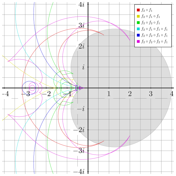
Figure 1. The shaded area is $U_{3}$. Those parameters $\lambda$ for which $g_{\lambda}$ has an indifferent fixed point for different $g\in H_{3}$ are colored according to the legend.

The remainder of the proof of Theorem 3 now consists of providing explicit examples of nontrivial $g\in H_{\Delta}$ with a parameter $\lambda\in U_{\Delta}$ such that $g_{\lambda}$ has an indifferent fixed point for each $\Delta\in\{3,\dots,9\}$. For $\Delta=3$ the degree is sufficiently small such that we can accurately calculate all such parameters for low degree $g\in H_{3}$, see Figure 1. It is immediately clear that there are many parameters that lie inside $U_{3}$.

For larger $\Delta$ it quickly becomes intractable to calculate images like in Figure 1, but it remains possible, given some $g\in H_{\Delta}$, to accurately calculate those parameters $\lambda$ for which $g_{\lambda}$ has a parabolic fixed point of some given multiplier. Numerical approximations for such parameters inside $U_{\Delta}$ where the multiplier is $1$ are given in Table 1. These results prove Theorem 3.

Table 1. Given for each $\Delta\in\{3,\dots,9\}$ is a $g\in H_{\Delta}$ together with an approximation of a $\lambda\in U_{\Delta}$ such that $g_{\lambda}$ has a fixed point $z$ with $g_{\lambda}^{\prime}(z)=1$. An approximation is given for the absolute value of $\alpha$, where $\alpha$ is a solution to $\lambda=\frac{-\alpha\cdot{(\Delta-1)}^{\Delta-1}}{\left(\Delta-1+\alpha\right)^{\Delta}}$ of least absolute value. This value being less than $1$ confirms that $\lambda\in U_{\Delta}$, see (2).

$\Delta$	$g$	$\lambda$	$|\alpha|$
$3$	$f_{2}\circ f_{1}$	$0.7624680+2.5253695\,i$	$0.97581$
$4$	$f_{3}\circ f_{1}$	$0.37725715+1.21796118\,i$	$0.99987$
$5$	$f_{4}\circ f_{4}\circ f_{1}$	$-0.24803954+0.17613988\,i$	$0.98607$
$6$	$f_{5}\circ f_{5}\circ f_{1}$	$-0.19657017+0.14664968\,i$	$0.99630$
$7$	$f_{6}\circ f_{6}\circ f_{2}$	$-0.15604600+0.14898604\,i$	$0.97830$
$8$	$f_{7}\circ f_{7}\circ f_{2}$	$-0.13276176+0.12728769\,i$	$0.98408$
$9$	$f_{8}\circ f_{8}\circ f_{2}$	$-0.11587455+0.11090067\,i$	$0.98967$

5. Concluding remarks

It follows from Lemma 13 that the set of roots of $Z_{G}$ for all $G\in\mathcal{G}_{\Delta}$ accumulates at the boundary of $V_{\Delta}$, where

$$V_{\Delta}=\left\{\lambda:\text{$g_{\lambda}$ has exactly 1 attracting fixed point for all $g\in H_{\Delta}$ with $g\neq f_{1}^{N}$}\right\}.$$

Recall that we defined $D_{\Delta}$ to be the largest domain containing $0$ that is zero-free for all $G\in\mathcal{G}_{\Delta}$. In Section 3.2 we showed that parameters $\lambda$ with $|\lambda|<(\Delta-1)^{\Delta-1}/\Delta^{\Delta}$ lie in $V_{\Delta}$. In [SS05] it is shown that these $\lambda$ also lie in $D_{\Delta}$. It follows that $D_{\Delta}\subseteq V_{\Delta}$. By definition, we have $V_{\Delta}\subseteq U_{\Delta}$ and thus we can write

$$D_{\Delta}\subseteq V_{\Delta}\subseteq U_{\Delta},$$

where the last inclusion was shown to be strict for $3\leq\Delta\leq 9$ in this paper. Two obvious questions that remain open are whether $V_{\Delta}\neq U_{\Delta}$ for $\Delta\geq 10$ and whether $D_{\Delta}=V_{\Delta}$ for any $\Delta$.

Another question concerns the computational complexity of approximating the independence polynomial. Recall that for $\lambda\in D_{\Delta}$ there is an polynomial time algorithm to approximate $Z_{G}(\lambda)$ for $G\in\mathcal{G}_{\Delta}$ (see [PR17]). On the other hand, for non-real $\lambda$ outside $U_{\Delta}$ it was shown by Bezáková, Galanis, Goldberg and Štefankovič [BGGv18] that approximating $Z_{G}(\lambda)$ is #P-hard. The computational complexity of approximating $Z_{G}(\lambda)$ for $\lambda\in U_{\Delta}-V_{\Delta}$ remains to be studied. Given the similar definitions of the region $U_{\Delta}$ and $V_{\Delta}$, one might expect that approximating $Z_{G}(\lambda)$ for non-real $\lambda$ outside $V_{\Delta}$ is also #P-hard.

Appendix A Proof of Lemma 9

The proof that we present here is algebraic rather than analytic in nature. We view $\mathbb{C}[\lambda,z]$ as a subring of the ring $\mathbb{C}(\lambda)[z]$. This ring is Euclidian, so in particular it is a unique factorization domain. Therefore we can state the following simple lemma.

Lemma 14.

Let $p,q\in\mathbb{C}[\lambda,z]$ be coprime in $\mathbb{C}(\lambda)[z]$. Then there are only finitely many $\lambda\in\mathbb{C}$ such that the polynomials $p(\lambda,z)$ and $q(\lambda,z)$ viewed as elements of $\mathbb{C}[z]$ have common roots.

Proof.

Since $p,q$ are coprime in the Euclidian domain $\mathbb{C}(\lambda)[z]$, there exist elements $u,v\in\mathbb{C}(\lambda)[z]$ such that $u\cdot p+v\cdot q=1$. There exists an element $w\in\mathbb{C}[\lambda]$ such that the coefficients of $w\cdot u$ and $w\cdot v$ are elements of $\mathbb{C}[\lambda]$. It follows that for all $\lambda,z$ we have can write down the following equality of polynomials

$$w(\lambda)u(\lambda,z)\cdot p(\lambda,z)+w(\lambda)v(\lambda,z)\cdot q(\lambda,z)=w(\lambda).$$

We deduce now that if there is some pair $(\lambda_{0},z_{0})$ that is both a root of $p$ and $q$, then $\lambda_{0}$ is a root of $w$. Since $w$ has only finitely many roots, we deduce that only finitely many such $\lambda$ can exist. ∎

Before we prove Lemma 9, we recall some properties of the algebraic construction called the resultant. Namely, if $k$ is a field and $f,g\in k[x]$, then the resultant of $f$ and $g$, denoted by $\operatorname{Res}_{x}(f,g)$, is an integer polynomial in the coefficients of $f$ and $g$ with the property that $\operatorname{Res}_{x}(f,g)=0$ if and only if $f,g$ have a common factor in $k[x]$. One can read about the theory of resultants in many introductory texts on computational algebraic geometry, see e.g. [CLO07, Chapter 3, §5]. We now present a proof of Lemma 9.

Proof of Lemma 9.

We can assume that $p,q$ are coprime in $\mathbb{C}(\lambda)[z]$. Let $U$ be a neighborhood of $\lambda_{0}$ together with a map $w:U\to\widehat{\mathbb{C}}$ that has the properties described in Definition 5. We can assume that the map $w$ avoids $\infty$. The holomorphic map

$$\lambda\mapsto f_{\lambda}^{\prime}(w(\lambda))$$

is an open map with constant absolute value and is thus constant on $U$, say equal to $\alpha$ with $|\alpha|=1$. Note that we can write

$$f_{\lambda}^{\prime}(z)=\frac{s(\lambda,z)}{t(\lambda,z)},$$

with $s,t\in\mathbb{C}[\lambda,z]$ coprime in $\mathbb{C}(\lambda)[z]$. Define the following polynomials

$$l(\lambda,z)=p(\lambda,z)-z\cdot q(\lambda,z)\quad\text{ and }\quad m(\lambda,z)=s(\lambda,z)-\alpha\cdot t(\lambda,z).$$

It follows from Lemma 14 that for all but finitely many $\lambda$ we have that $f_{\lambda}(z)=z$ if and only if $l(\lambda,z)=0$ and similarly for all but finitely many $\lambda$ we have $f_{\lambda}^{\prime}(z)=\alpha$ if and only if $m(\lambda,z)=0$. Consider the polynomial

$$R(\lambda)=\operatorname{Res}_{z}(l,m).$$

Note that $R(\lambda)\in\mathbb{C}[\lambda]$. Since for all but finitely many $\lambda\in U$ the polynomials $m(\lambda,z)$ and $l(\lambda,z)$ have a common root, namely $w(\lambda)$, we find that $R(\lambda)$ has infinitely many roots and is constantly $0$ as a result. This means that for all $\lambda\in\mathbb{C}$ the polynomials $m(\lambda,z)$ and $l(\lambda,z)$ have a common root. This again means that for all but finitely many $\lambda$ there is some $z\in\mathbb{C}$ such that $f_{\lambda}(z)=z$ and $f^{\prime}_{\lambda}(z)=\alpha$, where we now consider $f_{\lambda}$ to be defined for every complex parameter $\lambda$. This concludes the proof. ∎

References

- [Bar16] Alexander Barvinok, Combinatorics and complexity of partition functions, Algorithms and Combinatorics, vol. 30, Springer, Cham, 2016. MR 3558532
- [BC18] Ferenc Bencs and Péter Csikvári, Note on the zero-free region of the hard-core model, arXiv e-prints (2018), arXiv:1807.08963.
- [BGGv18] Ivona Bezáková, Andreas Galanis, Leslie Ann Goldberg, and Daniel Štefankovič, Inapproximability of the independent set polynomial in the complex plane, STOC’18—Proceedings of the 50th Annual ACM SIGACT Symposium on Theory of Computing, ACM, New York, 2018, pp. 1234–1240. MR 3826331
- [CLO07] David Cox, John Little, and Donal O’Shea, Ideals, varieties, and algorithms, third ed., Undergraduate Texts in Mathematics, Springer, New York, 2007, An introduction to computational algebraic geometry and commutative algebra. MR 2290010
- [LY52a] T. D. Lee and C. N. Yang, Statistical theory of equations of state and phase transitions. I. Theory of condensation, Physical Rev. (2) 87 (1952), 404–409. MR 0053028
- [LY52b] by same author, Statistical theory of equations of state and phase transitions. II. Lattice gas and Ising model, Physical Rev. (2) 87 (1952), 410–419. MR 0053029
- [McM94] Curtis T. McMullen, Complex dynamics and renormalization, Annals of Mathematics Studies, vol. 135, Princeton University Press, Princeton, NJ, 1994. MR 1312365
- [MnSS83] R. Mañé, P. Sad, and D. Sullivan, On the dynamics of rational maps, Ann. Sci. École Norm. Sup. (4) 16 (1983), no. 2, 193–217. MR 732343
- [PR17] Viresh Patel and Guus Regts, Deterministic polynomial-time approximation algorithms for partition functions and graph polynomials, SIAM J. Comput. 46 (2017), no. 6, 1893–1919. MR 3738853
- [PR19] Han Peters and Guus Regts, On a conjecture of sokal concerning roots of the independence polynomial, Michigan Math. J. (2019), Advance publication.
- [She85] J. B. Shearer, On a problem of Spencer, Combinatorica 5 (1985), no. 3, 241–245. MR 837067
- [Sok01] A. D. Sokal, A personal list of unsolved problems concerning lattice gases and antiferromagnetic Potts models, Markov Process. Related Fields 7 (2001), no. 1, 21–38, Inhomogeneous random systems (Cergy-Pontoise, 2000). MR 1835744
- [SS05] Alexander D. Scott and Alan D. Sokal, The repulsive lattice gas, the independent-set polynomial, and the Lovász local lemma, J. Stat. Phys. 118 (2005), no. 5-6, 1151–1261. MR 2130890
- [Wei06] Dror Weitz, Counting independent sets up to the tree threshold, STOC’06: Proceedings of the 38th Annual ACM Symposium on Theory of Computing, ACM, New York, 2006, pp. 140–149. MR 2277139