Spin Hall effect of light in a random medium

Abstract

We show that optical beams propagating in transversally disordered materials exhibit a spin Hall effect and a spin-to-orbital conversion of angular momentum as they deviate from paraxiality. We theoretically describe these phenomena on the basis of the microscopic statistical approach to light propagation in random media, and show that they can be detected via polarimetric measurements under realistic experimental conditions.

In random media, exploiting of the common wave-like nature of photons and electrons has led to the observation of several optical analogues of condensed-matter phenomena. Well known examples include fluctuations of photon conductance Scheffold98 , weak localization of light Albada85 ; Wolf85 or optical Anderson insulators Berry97 ; Schwartz07 . In Faraday active materials, transverse diffusive currents resembling the Hall effect were also predicted Tiggelen95 and observed Rikken96 , and characterizations of photon localization under partially broken time-reversal symmetry were reported Bromberg16 ; Maret18 , in analogy with charged electrons in magnetic fields Beenakker97 . Recently, the propagation of paraxial light through disordered arrays of helical waveguides even allowed to realize a topological photonic Anderson insulator Stutzer18 .

A currently open question is whether spin-orbit interactions (SOI) of light, i.e. the coupling between the spatial and polarization degrees of freedom of an optical wavefront, can be achieved in a random medium. A positive answer would be appealing, since in solids spin-orbit coupling is known to affect quantum transport, giving rise for instance to weak anti-localization or driving random systems to other symmetry classes Evers08 . SOI could also be used as a tool to design novel types of topological insulators Lu14 ; Ozawa18 in random environments. As it turns out, optical SOI naturally arise in inhomogeneous media. One of their manifestations is the optical spin Hall effect (SHE), which refers to helicity dependent sub-wavelength shifts of the trajectory of circularly polarized beams, in analogy with their electronic counterparts Sinova15 . Originally identified for light refracted or reflected at interfaces (Imbert-Fedorov effect) Fedorov55 ; Imbert72 and later in gradient-index materials (optical Magnus effect) Dooghin92 ; Liberman92 , the SHE of light was recently described at a more general level on the basis of a geometric Berry phase Bliokh04 ; Onoda04 . On the experimental side, pioneering measurements at interfaces were carried out in optics Hosten08 and plasmonics Gorodetski12 , and nowadays SOI of light have become a promising tool for the generation of vortex beams or the optical control of nano-optical systems Cardano15 ; Bliokh15 . In this Letter, we demonstrate that the SHE of light is generically present in transversally disordered media, a geometry recently exploited in the context of wave localization Boguslawski17 ; Schwartz07 ; Boguslawski13 ; Stutzer18 . We find that the SHE emerges for beams deviating from the paraxial limit and exists even if the disorder is statistically homogeneous. While the SHE is naturally small, we show that it can be magnified and detected via polarimetric measurements under realistic experimental conditions.

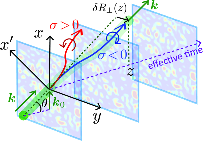
Figure 1: We consider the propagation of a collimated beam of wave vector ${\boldsymbol{k}}$ through a medium spatially disordered in the $(x,y)$ plane and homogeneous along the optical axis $z$. As soon as the transverse wave vector ${\boldsymbol{k}}_{0}$ (along the $x$-axis) is nonzero, the disorder-average centroid of the coherent mode is shifted laterally along $y$ as $z$ increases (spin Hall effect). The shift is proportional to the beam helicity $\sigma$ and shows up even if the medium is statistically homogeneous.

In an inhomogeneous medium of permittivity distribution $\epsilon({\boldsymbol{r}})$, it was shown from semi-classical considerations that the mean coordinate R and dimensionless wave vector $\textbf{P}={\boldsymbol{k}}c/\omega$ of an optical beam obey $\dot{\textbf{R}}=\textbf{P}/P-(\sigma c/\omega P^{3})\textbf{P}\times\dot{\textbf{P}}$ and $\dot{\textbf{P}}={\boldsymbol{\nabla}}{\sqrt{\epsilon(\boldsymbol{R})}}$, where $\sigma$ is the beam helicity, $\omega$ the optical frequency, $c$ the vacuum speed of light and the dot denotes derivation with respect to the optical path length Liberman92 ; Bliokh04 ; Onoda04 . The first equation of motion emphasizes the spin Hall effect of light, an helicity dependent, sub-wavelength spatial shift of the beam. Suppose now that $\epsilon({\boldsymbol{r}})$ describes a random medium. If the latter is statistically isotropic, the beam momentum distribution and permittivity gradient are typically uncorrelated so that disorder averaging leads to $\dot{\textbf{R}}=\textbf{P}/P$: no shift survives on average. To observe a finite optical SHE, a statistically anisotropic disorder should be used. A simple configuration fulfilling this requirement is illustrated in Fig. 1: a monochromatic collimated beam, of wave vector ${\boldsymbol{k}}$ lying in the $(x,z)$ plane, propagates in a material with disorder only in the transverse plane ${\boldsymbol{r}}_{\perp}=(x,y)$: $\epsilon({\boldsymbol{r}})=\epsilon({\boldsymbol{r}}_{\perp})$. This geometry has been much studied in the framework of the paraxial wave equation, in which the coordinate $z$ plays the role of an effective propagation time Raedt89 . By going beyond the paraxial description, we find that beams carrying a finite helicity are laterally shifted as soon as their transverse wave vector ${\boldsymbol{k}}_{0}=k_{0}\textbf{e}_{x}$ is nonzero. This shift, which constitutes the optical SHE in a random medium, is visible in the so-called coherent mode, namely before the beam has been converted into a diffusive halo due to multiple scattering Sheng95 . Specifically, for an incoming beam of complex polarization vector ${\boldsymbol{\mathcal{\varepsilon}}}(z=0)=(\textbf{e}_{x^{\prime}}+e^{i\phi}\textbf{e}_{y})/\sqrt{2}$, ($\textbf{e}_{x^{\prime}}\equiv\textbf{e}_{y}\times{\boldsymbol{k}}/k$), we find a lateral shift (see Fig. 1)

$$\delta R_{\perp}(z)=-\frac{\sigma}{k_{0}}\left[1-\frac{1}{\text{cosh}(z/2z_{\text{SH}})}\right]$$ (1)

at small angle of incidence $\theta\simeq k_{0}/k\equiv\hat{k}_{0}$, with $\sigma=\sin\phi$ the beam helicity, $\sigma=+1$ $(-1)$ for left(right)-handed circular polarization footnote2 . The shift continuously increases as the beam propagates deeper in the random medium, until it saturates at $\sim 1/k_{0}$ beyond a characteristic time $z_{\text{SH}}\equiv z_{s}/\hat{k}_{0}^{2}$, where $z_{s}$ is the scattering mean free time Cherroret18 . The SHE vanishes for linearly polarized light, $\sigma=0$. Note here the peculiarities of the transverse disorder scheme: the spin Hall shift evolves in time and is on the order of the transverse wavelength $1/k_{0}$, and not $1/k$ like in conventional shifts at interfaces Bliokh15 .

To demonstrate Eq. (1), a possible strategy consists in directly averaging the aforementioned semi-classical equations over disorder configurations. Because this approach seems hardly generalizable to higher orders of perturbation theory however, we have used a more general vector wave treatment based on the exact optical Dyson equation in random media Sheng95 ; Stephen86 ; vanTiggelen96 ; Busch05 . Within this framework, we consider the evolution of the coherent mode in a transversally disordered material illuminated at $z=0$ by a collimated beam of electric field profile $\textbf{E}({\boldsymbol{r}}_{\perp},z=0)$. To describe this evolution, we define the normalized intensity, $\hat{I}({\boldsymbol{r}}_{\perp},z)\equiv I({\boldsymbol{r}}_{\perp},z)/I_{\text{tot}}(z)$, where $I({\boldsymbol{r}}_{\perp},z)\equiv|\langle\textbf{E}({\boldsymbol{r}}_{\perp},z)\rangle|^{2}$, $I_{\text{tot}}(z)\equiv\int d^{2}{\boldsymbol{r}}_{\perp}|\langle\textbf{E}({\boldsymbol{r}}_{\perp},z)\rangle|^{2}$ and the brackets refer to disorder averaging. The normalization is here introduced so to work with a conservative quantity, as in a random medium the intensity of the coherent mode decays exponentially beyond the scattering mean free path Sheng95 , an effect that we will discuss later on. The components $E_{j}$ ($j=x,y,z$) of the complex electric field at coordinate $z$ obey the Helmholtz equation

$$\left[\Delta\delta_{ij}\!-\!\nabla_{i}\nabla_{j}\!+\!k^{2}\delta_{ij}(1\!+\!\delta\epsilon({\boldsymbol{r}}_{\perp})/\bar{\epsilon})\right]E_{j}(\boldsymbol{r}_{\perp},z)=0.$$ (2)

Disorder is here encoded in random permittivity fluctuations $\delta\epsilon({\boldsymbol{r}}_{\perp})=\epsilon({\boldsymbol{r}}_{\perp})-\overline{\epsilon}$ around a mean value $\overline{\epsilon}$. We choose them Gaussian distributed and correlated according to the general form $\overline{\delta\epsilon({\boldsymbol{r}}_{\perp})\delta\epsilon({\boldsymbol{r}}_{\perp}^{\prime})}/{\bar{\epsilon}^{2}}=B({\boldsymbol{r}}_{\perp}-{\boldsymbol{r}}_{\perp}^{\prime})$, where $B$ is an isotropic decaying function. The disorder average field, $\langle E_{i}({\boldsymbol{r}}_{\perp},z)\rangle=\int d^{2}{\boldsymbol{k}}_{\perp}/(2\pi)^{2}\langle t_{ij}({\boldsymbol{k}}_{\perp},z)\rangle E_{j}({\boldsymbol{k}}_{\perp},z\!=\!0)e^{i{\boldsymbol{k}}_{\perp}\!\cdot{\boldsymbol{r}}_{\perp}}$, is governed by the average transmission coefficient of the medium, $\langle t_{ij}({\boldsymbol{k}}_{\perp},z)\rangle=2i(k^{2}-{\boldsymbol{k}}_{\perp}^{2})^{1/2}\langle G_{ij}({\boldsymbol{k}}_{\perp},z)\rangle$, where ${G}_{ij}$ is the Green’s tensor of Eq. (2) Feng94 . To find its disorder average, we have diagonalized the Dyson equation for its Fourier transform, $\langle\textbf{G}({\boldsymbol{k}}_{\perp},k_{z})\rangle=[\textbf{G}^{(0)}({\boldsymbol{k}}_{\perp},k_{z})^{-1}-\boldsymbol{\Sigma}({\boldsymbol{k}}_{\perp},k_{z})]^{-1}$, where $G^{(0)}_{ij}({\boldsymbol{k}}_{\perp},k_{z})=(\delta_{ij}-\hat{k}_{i}\hat{k}_{j})/(k^{2}-{\boldsymbol{k}}_{\perp}^{2}-k_{z}^{2}+i0^{+})$ and the self-energy tensor is evaluated at the level of the Born approximation: $\Sigma_{ij}({\boldsymbol{k}}_{\perp},k_{z})=\int d^{2}{\boldsymbol{k}}_{\perp}^{\prime}/(2\pi)^{2}B({\boldsymbol{k}}_{\perp}-{\boldsymbol{k}}_{\perp}^{\prime})G^{(0)}_{ij}({\boldsymbol{k}}^{\prime}_{\perp},k_{z})$ Cherroret18 . To make the calculation concrete, we model the incident light by a collimated Gaussian beam $\textbf{E}({\boldsymbol{r}}_{\perp},z=0)=2/(\sqrt{\pi}w_{0})\exp(-2r_{\perp}^{2}/w_{0}^{2}+i{\boldsymbol{k}}_{0}\cdot{\boldsymbol{r}}_{\perp}){\boldsymbol{\mathcal{\varepsilon}}}(z=0)$ with unit polarization vector ${\boldsymbol{\mathcal{\varepsilon}}}(z=0)=(\textbf{e}_{x^{\prime}}+e^{i\phi}\textbf{e}_{y})/\sqrt{2}$ and waist $w_{0}$ such that $w_{0}k_{0}\gg 1$. By using this initial state and the solution of the Dyson equation for the Green’s tensor, we find, at leading order in $\hat{k}_{0}\ll 1$ (small $\theta)$:

$$\hat{I}({\boldsymbol{r}}_{\perp},z)=\hat{I}({\boldsymbol{r}}_{\perp}-\textbf{R}_{\perp}(z),0).$$ (3)

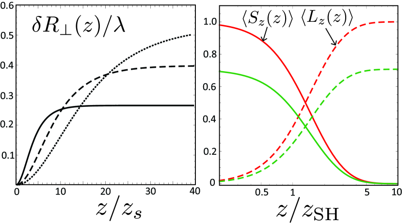
Figure 2: Left: spin Hall shift versus $z/z_{s}$ ($z_{s}$ mean free time) of a right-handed circularly polarized beam, for $\hat{k}_{0}=0.3$, $0.4$ and $0.6$ from top to bottom. Right: spin-to-orbital angular momentum conversion. As $z$ increases, the $z$-component of the spin angular momentum $\langle S_{z}(z)\rangle$ (solid curves) decreases and the beam acquires a finite orbital angular momentum $\langle L_{z}(z)\rangle$ (dashed curves), with the sum $\langle S_{z}(z)\rangle+\langle L_{z}(z)\rangle=1$ conserved. Upper and lower curves correspond to $\sigma=1$ and $0.7$, respectively.

This result describes a shift of the centroid $\textbf{R}_{\perp}(z)\equiv\int d^{2}{\boldsymbol{r}}_{\perp}{\boldsymbol{r}}_{\perp}I({\boldsymbol{r}}_{\perp},z)/I_{\text{tot}}(z)$ as the beam evolves along the effective time axis $z$. The centroid shift is

$$\textbf{R}_{\perp}(z)=\hat{\boldsymbol{k}}_{0}z+\delta R_{\perp}(z){\boldsymbol{e}}_{y}.$$ (4)

In Eq. (4), the first term on the right-hand side is the usual geometrical-optics contribution, while the second term is the spin Hall effect of light, where $\delta R_{\perp}(z)$ is given by Eq. (1) and the scattering mean free time follows from the angular average of the disorder power spectrum, $z_{s}^{-1}=k^{3}\langle B(k_{0},\hat{{\boldsymbol{k}}}_{\perp}\!\!-\!\!\hat{{\boldsymbol{k}}}^{\prime}_{\perp})\rangle_{\hat{{\boldsymbol{k}}}^{\prime}_{\perp}}/4$ footnote1 . The left panel in Fig. 2 shows $\delta R_{\perp}(z)$ versus $z$ in units of $\lambda=2\pi/k$, for three values of $\hat{k}_{0}$. Its asymptotic limit, $\delta R_{\perp}(z\gg z_{\text{SH}})=-\sigma/k_{0}$, increases with decreasing ${k}_{0}$. Note that unlike the beam centroid, the mean momentum ${\boldsymbol{k}}$ remains fixed during propagation, as the coherent mode by definition describes the unscattered part of the optical signal.

Often, optical SHE can alternatively be interpreted as a conversion of angular optical momentum: as the beam propagates in the inhomogeneous material, its spin angular momentum is converted into an orbital angular momentum Bliokh15 . It turns out that, in a random medium, this picture holds for the coherent mode as well. To show this, we have computed the angular momentum of the coherent mode, using the statistical approach described above. At small $\hat{k}_{0}$, the latter decomposes into an orbital contribution, $\langle\textbf{L}(z)\rangle\equiv-i\int d^{2}{\boldsymbol{r}}_{\perp}\langle E_{i}^{*}({\boldsymbol{r}}_{\perp},z)\rangle({\boldsymbol{r}}\times\nabla)\langle E_{i}({\boldsymbol{r}}_{\perp},z)\rangle/I_{\text{tot}}(z)$, and a spin contribution, $\langle\textbf{S}(z)\rangle\equiv-i\int d^{2}{\boldsymbol{r}}_{\perp}\langle\textbf{E}^{*}({\boldsymbol{r}}_{\perp},z)\rangle\times\langle\textbf{E}({\boldsymbol{r}}_{\perp},z)\rangle/I_{\text{tot}}(z)$ Alonso12 . From the solution of the Dyson equation, we derive the transparent relation $\langle\textbf{L}(z)\rangle=\delta\textbf{R}_{\perp}(z)\times{\boldsymbol{k}}$, which shows that the SHE can be regarded as the emergence of a finite orbital momentum. Of peculiar interest are the axial components $L_{z}(z)$ and $S_{z}(z)$, which explicitly read

$$\langle L_{z}(z)\rangle\!=\!\sigma\!\left[1\!-\!\frac{1}{\text{cosh}(z/2z_{\text{SH}})}\right]\!,\ \langle S_{z}(z)\rangle\!=\!\sigma\!-\!\langle L_{z}(z)\rangle.$$ (5)

$\langle L_{z}(z)\rangle$ and $\langle S_{z}(z)\rangle$ are displayed in the right panel of Fig. 2 as a function of $z$. As $z$ increases, the SOI mediated by the random medium convert $\langle S_{z}\rangle$ into $\langle L_{z}\rangle$ with no net angular momentum transferred to the random medium, which only acts as an intermediary. Note that unlike conversions previously reported in inhomogeneous anisotropic materials ($q$ plates) Marrucci06 , here the spatial beam shape is preserved, see Eq. (3), so that the orbital angular momentum is “external”, i.e. not associated with a vortex. In our system, the exact conservation of the $z$-component of the total angular momentum stems from the global, statistical rotational symmetry around the $z$-axis. The spin-to-orbital conversion described here also indicates that the mean polarization of the incoming beam is not fixed, but evolves during propagation. From the Fourier component $\langle\textbf{E}({\boldsymbol{k}}_{\perp}\simeq{\boldsymbol{k}}_{0},z)\rangle\propto{\boldsymbol{\mathcal{\varepsilon}}}(z)$, we extract the explicit expression of the mean polarization vector ${\boldsymbol{\mathcal{\varepsilon}}}(z)$. For an initial beam with ${\boldsymbol{\mathcal{\varepsilon}}}(z=0)=(\textbf{e}_{x^{\prime}}+e^{i\phi}\textbf{e}_{y})/\sqrt{2}$, we find:

$${\boldsymbol{\mathcal{\varepsilon}}}(z)=\frac{\textbf{e}_{x^{\prime}}+e^{i\phi}\exp(-z/2z_{\text{SH}})\textbf{e}_{y}}{\sqrt{1+\exp(-z/z_{\text{SH}})}}.$$ (6)

Trajectories of the electric field vector in the plane $(x^{\prime},y)$ pertained to Eq. (6) are represented in Fig. 3 at increasing values of $z$ for $\sigma=1$, $0.7$ and $0$ (circular, elliptic and linear polarization, respectively). Due to the spin-to-orbital angular momentum conversion, the beam always end up linearly polarized along $x^{\prime}$ beyond the spin Hall time $z_{\text{SH}}$, whatever the initial polarization state. Interestingly, the polarization vector of initially linearly polarized light rotates as well, although no SHE arises in this case.

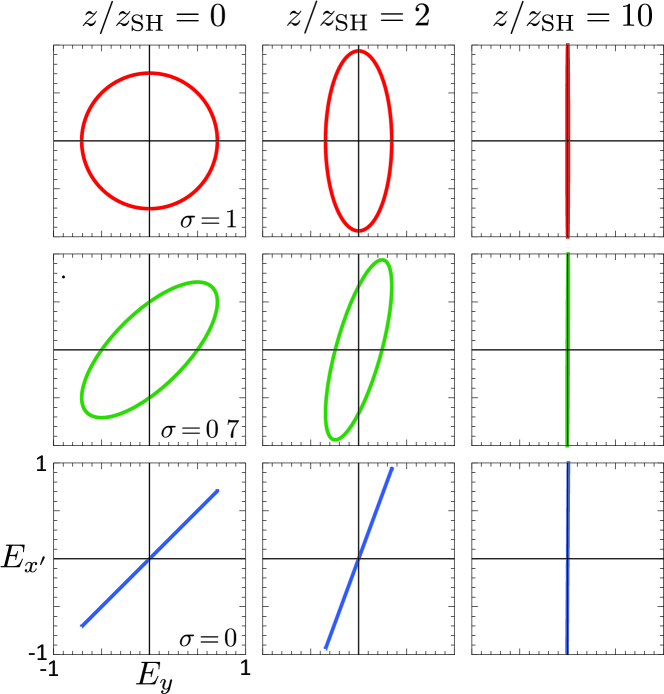
Figure 3: Real time evolution of the electric field vector $(E_{x^{\prime}},E_{y})$ at increasing $z$, for $\sigma=1$ (top panels, circular polarization), $0.7$ (middle panels, elliptic polarization) and $0$ (lower panels, linear polarization). Whatever the initial polarization state, the beam always end up linearly polarized along $x^{\prime}$ when $z\gg z_{\text{SH}}$.

We finally present an experimental proposal for measuring the SHE of light in a random medium. As seen from Eq. (1), in the transverse disorder scheme the maximum shift is $\sim 1/k_{0}$, which is much larger than $1/k$ at small angle of incidence. Unfortunately, this value is only reached at times $z>z_{\text{SH}}=z_{s}/\hat{k}_{0}^{2}$, typically longer than the mean free time $z_{s}$. In this regime, the signal is exponentially attenuated because most photons have been scattered out of the initial mode and converted into a diffusive signal: $I({\boldsymbol{r}}_{\perp},z)\propto\exp(-z/z_{s})$ Akkermans07 . To circumvent this issue, a solution is to magnify the SHE by means of a polarimetric measurement, in the spirit of previous works on optical shifts at interfaces Hosten08 ; Gorodetski12 . This strategy is based on a technique analogous to weak measurements in quantum mechanics Aharonov88 ; Duck89 which, as we show now, can be applied to the coherent mode of a random medium as well. For this purpose, we suppose that the incoming beam is linearly polarized along $x^{\prime}$, ${\boldsymbol{\mathcal{\varepsilon}}}(z=0)=\textbf{e}_{x^{\prime}}$. In this particular configuration, the mean polarization ${\boldsymbol{\mathcal{\varepsilon}}}(z)$ remains fixed, but its spatial polarization distribution, $\propto\langle\textbf{E}^{*}({\boldsymbol{r}}_{\perp},z)\rangle\times\langle\textbf{E}({\boldsymbol{r}}_{\perp},z)\rangle\propto\textbf{e}_{x^{\prime}}\times{\boldsymbol{r}}_{\perp}\exp(-2r_{\perp}^{2}/w_{0}^{2})$, is inhomogeneous: the core of the beam is linearly polarized while the wings $|{\boldsymbol{r}}_{\perp}|\sim w_{0}$ are circularly polarized with opposite helicities, as illustrated in Fig. 4(a). This implies that by detecting light at $z$ in the polarization channel ${\boldsymbol{\mathcal{\varepsilon}}}_{\text{out}}=(\textbf{e}_{y}+i\delta\textbf{e}_{x^{\prime}})/\sqrt{1+\delta^{2}}$, with $\delta$ a small real number [Fig. 4(a)], a spin Hall shift on the order of $w_{0}$ can be detected. Precisely, we find that the beam centroid, now defined as $\textbf{R}_{\perp}=\int d^{2}{\boldsymbol{r}}_{\perp}{\boldsymbol{r}}_{\perp}|\langle{\boldsymbol{\mathcal{\varepsilon}}}_{\text{out}}^{*}\cdot\textbf{E}({\boldsymbol{r}}_{\perp},z)\rangle|^{2}/\int d^{2}{\boldsymbol{r}}_{\perp}|\langle{\boldsymbol{\mathcal{\varepsilon}}}_{\text{out}}^{*}\cdot\textbf{E}({\boldsymbol{r}}_{\perp},z)\rangle|^{2}$, is given by:

$$\delta R_{\perp}(\delta,z)\!=\!-\frac{\delta}{k_{0}}\frac{1\!-\!\exp(-z/2z_{\text{SH}})}{\delta^{2}\!+\!2[1\!-\!\exp(-z/2z_{\text{SH}})]^{2}/(w_{0}k_{0})^{2}}.$$ (7)

As compared to the case where no polarimetric measurement is performed, Eq. (1), the SHE can now be enhanced by several orders of magnitude via the parameter $\delta$, with a maximum value $\delta R_{\perp}(z)\sim w_{0}$ for $z\gg z_{\text{SH}}$ and $\delta\simeq 1/w_{0}k_{0}$ Gorodetski12 . To establish the practical conditions under which the SHE can be measured though, we must additionally account for the attenuation of the coherent mode. This attenuation is both due to the polarimetric measurement, which only selects a fraction $\delta^{2}$ of the intensity and, as discussed above, to multiple scattering. The latter depletes exponentially the coherent mode, which becomes weaker than the diffusive signal emerging around after a few mean free times $z_{s}$.

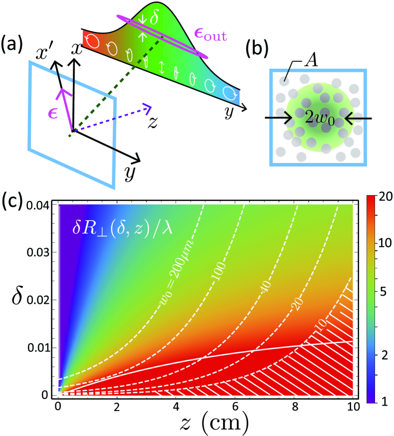
Figure 4: (a) When propagating in disorder, beams polarized along $\textbf{e}_{x^{\prime}}$ acquire an inhomogeneous polarization structure with circularly polarized wings. By detecting light along ${\boldsymbol{\mathcal{\varepsilon}}}_{\text{out}}\propto(\textbf{e}_{y}+i\delta\textbf{e}_{x^{\prime}})$ with $\delta\ll 1$, a magnified spin Hall shift can be observed. (b) To estimate the mean free time $z_{s}$, we consider a random array of guides of section $A$, surface density $\rho$ and relative refractive index $\delta n/n$. Taking $\lambda=532$ nm, $\delta n/n=7.10^{-4}$, $n=1.5$, $\hat{k}_{0}=0.57$, $A=20\mu$m² and $\rho=0.02\mu$m^-2, we find $z_{s}\simeq 1$ cm. (c) Density plot of the spin Hall shift in wavelength units, Eq. (7), versus $z$ and $\delta$. Dashed white curves indicate the boundary where the constraint (8) becomes an equality for various beam waists $w_{0}$. The SHE is only detectable in the region lying above these curves. The solid curve indicates the level set $\delta R_{\perp}=20\lambda$.

This phenomenon, which constitutes the main limitation to a measurement of the SHE, imposes constraints on $z$ and $\delta$. To find them, we compare the intensity per unit surface of the coherent mode, $I\simeq\delta^{2}/(\pi w_{0}^{2}/2)\exp(-z/z_{s})$ with $I_{d}$, the diffusive signal around. The latter was computed in Cherroret18 in the geometry of transverse disorder: $I_{d}\simeq[1-\exp(-z/z_{p})]/(8\pi Dz)$, where $z_{p}=8z_{s}/5\hat{k}_{0}^{4}$ and the diffusion coefficient $D=\hat{k}_{0}^{2}z_{s}/2$ Cherroret18 . The constraint $I>I_{d}$ then reads:

$$\frac{w_{0}^{2}}{zz_{s}}[1-\exp(-z/z_{p})]<8\hat{k}_{0}^{2}\delta^{2}\exp(-z/z_{s}).$$ (8)

From this criterion, it appears that the beam waist $w_{0}$ should be as small as possible. For a realistic estimation, we consider a medium consisting of a random array of uniformly distributed guides of surface density $\rho$, relative refractive index $\delta n/n$ and Gaussian profile of section $A$, $B({\boldsymbol{k}}_{\perp})=\rho(A\delta n/n)^{2}\exp(-{\boldsymbol{k}}_{\perp}^{2}A/4\pi)$, a type of disorder easy to imprint on glass Bellec12 ; Bellec17 [Fig. 4(b)]. With this model we find the mean free time from the Born approximation: $z_{s}^{-1}=\rho k^{2}(\delta n/n)^{2}A^{3/2}/4\hat{k}_{0}$. Using this expression, we show in Fig. 4(c) a density plot of the spin Hall shift versus $(z,\delta)$, Eq. (7), obtained for $z_{s}\simeq 1$ cm. For a given waist $w_{0}$, the range of parameters where the inequality (8) is satisfied lies above the dashed curve, as explicitly indicated by the shaded area for $w_{0}=10\mu$m. This analysis suggests that for $\delta\sim 10^{-2}$, a shift on the order of $20\lambda$ (level set indicated by the solid curve) could be detected for $w_{0}\sim 10-40\mu$m.

To conclude, we have demonstrated the spin Hall effect of light in transversally disordered media, starting from the general statistical treatment of wave propagation in random media. We have also proposed a practical experimental configuration where an amplified SHE can be detected via polarimetric measurements. Our study constitutes a first step toward a general description of SOI of light in random media, where they could be exploited to achieve novel regimes of wave transport or engineer gauge fields for photons.

NC thanks Cyriaque Genet and Matthieu Bellec for useful advice and comments.

References

- (1) F. Scheffold and G. Maret, Phys. Rev. Lett. 81, 5800 (1998).
- (2) M. P. Van Albada and A. Lagendijk, Phys. Rev. Lett. 55, 2692 (1985).
- (3) P. E. Wolf and G. Maret, Phys. Rev. Lett. 55, 2696 (1985).
- (4) M. V. Berry and S. Klein, Eur. J. of Phys. 18, 222 (1997).
- (5) T. Schwartz, G. Bartal, S. Fishman, and M. Segev, Nature 446, 52 (2007).
- (6) Bart A. van Tiggelen Phys. Rev. Lett. 75, 422 (1995).
- (7) G. L. J. A. Rikken and B. A. van Tiggelen, Nature 381, 54 (1996).
- (8) Y. Bromberg, B. Redding, S. M. Popoff, and H. Cao, Phys. Rev. A 93, 023826 (2016).
- (9) L. Schertel, O. Irtenkauf, C. M. Aegerter, G. Maret, and G. J. Aubry, arXiv:1812.06447 (2019).
- (10) C. W. J. Beenakker, Rev. Mod. Phys. 69, 731 (1997).
- (11) S. Stützer, Y. Plotnik, Y. Lumer, P. Titum, N. H. Lindner, M. Segev, M. C. Rechtsman, and A. Szameit, Nature 560, 461 (2018).
- (12) F. Evers and A. D. Mirlin, Rev. Mod. Phys. 80, 1355 (2008).
- (13) L. Lu, J. D. Joannopoulos, and M. Soljačić, Nature Photonics 8, 821 (2014).
- (14) T. Ozawa, H. M. Price, A. Amo, N. Goldman, M. Hafezi, L. Lu, M. Rechtsman, D. Schuster, J. Simon, O. Zilberberg, and I. Carusotto, arXiv:1802.04173 (2018).
- (15) J. Sinova, S. O. Valenzuela, J. Wunderlich, C. H. Back, and T. Jungwirth, Rev. Mod. Phys. 87, 1213 (2015).
- (16) F. I. Fedorov, Dokl. Akad. Nauk SSR 105, 465 (1955).
- (17) C. Imbert, Phys. Rev. D 5, 787 (1972).
- (18) A. V. Dooghin, N. D. Kundikova, V. S. Liberman and B. Y. Zel’dovich, Phys. Rev. A 45, 8204 (1992).
- (19) V. S. Liberman and B. Y. Zel’dovich, Phys. Rev. A 46, 5199 (1992).
- (20) K. Yu. Bliokh and Y. P. Bliokh, Phys. Lett. A 333, 181 (2004).
- (21) M. Onoda, S. Murakami, and N. Nagaosa, Phys. Rev. Lett. 93, 083901 (2004).
- (22) O. Hosten and P. Kwiat P, Science 319 787 (2008).
- (23) Y. Gorodetski, K. Y. Bliokh, B. Stein, C. Genet, N. Shitrit, V. Kleiner, E. Hasman, and T. W. Ebbesen, Phys. Rev. Lett. 109, 013901 (2012).
- (24) F. Cardano and L. Marrucci, Nature Photonics 9, 776 (2015).
- (25) K. Y. Bliokh, F. J. Rodríguez-Fortuo, F. Nori and A. V. Zayats, Nature Photonics 9, 796 (2015).
- (26) M. Boguslawski, S. Brake, D. Leykam, A. S. Desyatnikov, and C. Denz, Sci. Rep. 7, 10439 (2017).
- (27) M Boguslawski, S. Brake, J. Armijo, F. Diebel, P. Rose, and C. Denz, Opt. Express 21, 31713 (2013).
- (28) H. De Raedt, Ad Lagendijk, and P. de Vries, Phys. Rev. Lett. 62, 47 (1989).
- (29) P. Sheng, Introduction to Wave Scattering, Localization, and Mesoscopic Phenomena, (Academic Press, San Diego,1995).
- (30) This expression does not include the constant Imbert-Fedorov shift possibly arising at the interface between the outside and the random medium.
- (31) N. Cherroret, Phys. Rev. A 98, 013805 (2018).
- (32) M. Stephen and G. Cwillich, Phys. Rev. B 34, 7564 (1986).
- (33) A. Lagendijk and B. A. van Tiggelen, Phys. Rep. 270, 143 (1996).
- (34) A. Lubatsch, J. Kroha, K. Busch, Phys. Rev. B 71, 184201 (2005).
- (35) R. Berkovits and S. Feng, Phys. Rep. 238, 135 (1994).
- (36) We here neglect the real part of the self energy, which shifts the average refractive index. We have checked than in usual transversally disordered media, in particular for the model in Fig. 4(b), this real part negligibly contributes to .
- (37) K. Y. Bliokh, A. Aiello, and M. A. Alonso, in The Angular Momentum of Light (eds. D. L. Andrews and M. Babiker) p. 174, Cambridge university press, Cambridge, 2012.
- (38) L. Marrucci, C. Manzo, and D. Paparo, Phys. Rev. Lett. 96, 163905 (2006).
- (39) E. Akkermans and G. Montambaux, Mesoscopic physics of electrons and photons, Cambridge university press, Cambridge, 2007.
- (40) Yakir Aharonov, David Z. Albert, and Lev Vaidman, Phys. Rev. Lett. 60, 1351 (1988).
- (41) I. M. Duck, P. M. Stevenson, and E. C. G. Sudarshan, Phys. Rev. D 40, 2112 (1989).
- (42) M. Bellec, P. Panagiotopoulos, D. G. Papazoglou, N. K. Efremidis, A. Couairon, and S. Tzortzakis Phys. Rev. Lett. 109, 113905 (2012).
- (43) M. Bellec, C. Michel, H. Zhang, S. Tzortzakis, and P. Delplace, Eur. Phys. Lett. 119, 14003 (2017).