Assessment of the Radiation Environment at Commercial Jet Flight Altitudes During GLE 72 on 10 September 2017 Using Neutron Monitor Data

Abstract

As a result of intense solar activity during the first ten days of September, a ground level enhancement occurred on September 10, 2017. Here we computed the effective dose rates in the polar region at several altitudes during the event using the derived rigidity spectra of the energetic solar protons. The contribution of different populations of energetic particles viz. galactic cosmic rays and solar protons, to the exposure is explicitly considered and compared. We also assessed the exposure of a crew members/passengers to radiation at different locations and at several cruise flight altitudes and calculated the received doses for two typical intercontinental flights. The estimated received dose during a high-latitude, 40 kft, $\sim$ 10 h flight is $\sim$ 100 $\mu$Sv.

Keywords:Solar eruptive events, Ground level enhancement, Neutron Monitor, Rigidity spectra of solar energetic protons,Exposure to radiation and received doses for crew members/passengers

For contact: alexander.mishev@oulu.fi

1 Introduction

Intense solar activity took place during the first ten days of September 2017. This time period was among the most flare productive of the ongoing solar cycle 24. The solar active region 12673 produced several X-class flares and coronal mass ejections (CMEs), leading to a moderate solar energetic particle (SEP) event, followed by a stronger, more energetic one, which was observed even at the ground level by several neutron monitors (NMs) (see the International GLE database http://gle.oulu.fi), i.e., the ground level enhancement (GLE) 72 event on September 10, 2017. The GLE 72 was related to an X8.2 solar flare, which peaked at 16:06 UT. It produced a gradual SEP event. At ground level, the event onset was observed at $\approx$ 16:15 UT (Fort Smith NM). Records of NMs with maximal count rate increases during the event are shown in Fig. 1. The maximal count rate increases were observed by high-altitude standard and lead-free, i.e. without $Pb$ producer, monitors at Concordia station, 75.06 S, 123.20 E, 3233 m above sea level (a.s.l.), (DOMC/DOMB, 10–15 $\%$ above the pre-increase levels), South Pole 2820 m a.s.l. (SOPO/SOPB, 5–8 $\%$) and at the sea level Forth Smith - FSMT ($\approx$ 6 $\%$). The lead free NMs (DOMB and SOPB) are more sensitive compared to standard NMs. In addition, high-altitude NMs are more sensitive than sea level NMs.

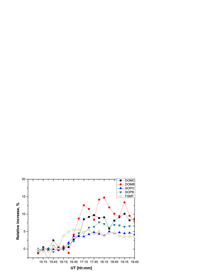
Figure 1: 15-min averaged count rate variations of NMs with maximal increases during GLE 72 on September 10, 2017. The DOMC and SOPO correspond to standard NMs at Dome-C and South Pole stations, DOMB and SOPB correspond to the lead free NMs at at Dome-C and South Pole stations. Data are available at http://gle.oulu.fi.

Strong SEP events can significantly change the radiation environment in the vicinity of Earth and in the Earth’s polar atmosphere, where the magnetospheric shielding is marginal (e.g. Spurny et al., 2002; Vainio et al., 2009, and references therein). While cosmic rays (CRs) of galactic origin permanently govern the radiation environment in the global atmosphere, particles of solar origin, specifically during strong SEP and GLE events can considerably enhance the flux of secondary CR particles in the atmosphere. Primary CR particles penetrate into the atmosphere and induce a complicated nuclear-electromagnetic-muon cascade, producing large amount of various types of secondary particles, viz. neutrons, protons, $\gamma$, $e^{-}$, $e^{+}$, $\mu^{-}$, $\mu^{+}$, $\pi^{-}$, $\pi^{+}$, distributed in a wide energy range, which eventually deposit their energy and ionize the ambient air (Bazilevskaya et al., 2008; Asorey et al., 2018). Hence, CR particles determine the complex radiation field at flight altitudes (Spurny et al., 1996; Shea and Smart, 2000).

Assessment of the radiation exposure, henceforth exposure, at typical flight altitudes is an important topic in the field of space weather (e.g. Baker, 1998; Latocha et al., 2009; Lilensten and Bornarel, 2009; Mertens et al., 2013; Mertens, 2016, and references therein). Individual accumulated doses of the cockpit and cabin crew are monitored and crew members are regarded as occupational workers (ICRP, 2007; EURATOM, 2014). The contribution of galactic cosmic rays (GCRs) to the exposure can be assessed by computations and/or using corresponding data sets for solar modulation and reference data (e.g. Menzel, 2010; Meier et al., 2018, and references therein), considering explicitly the altitude, geographic position, solar activity, geomagnetic conditions (Spurny et al., 2002; Shea and Smart, 2000; Tobiska et al., 2018). On the other hand, the assessment of exposure during GLEs can be rather complicated, because of their sporadic occurrence and a large variability of their spectra, angular distributions, durations and dynamics (Gopalswamy et al., 2012; Moraal and McCracken, 2012). For a precise computation of the exposure during a GLE event, it is necessary to possess appropriate information about the energy and angular distribution of the incoming high-energy particles (Kuwabara et al., 2006). Such computations are performed on a case-by-case basis for individual events (e.g. Sato et al., 2018).

Here, we computed the effective dose rates during GLE 72 at several cruise flight altitudes. We employed a recently developed model and procedure, the details are given in Mishev and Usoskin (2015) and Mishev et al. (2017). We calculated the exposure over the globe and the received doses of crew members/passengers for typical intercontinental flights.

2 Reconstruction of proton spectra for GLE 72 using NM data

Using a model briefly described below and actual records from the global NM network, we derived the rigidity spectra and angular distributions of solar protons for GLE 72, see details in Mishev et al. (2018). Estimates of GLE characteristics viz. rigidity/energy spectra and angular distributions can be performed using the NM data and a corresponding model of the global NM network response (e.g. Shea and Smart, 1982; Cramp et al., 1997). In this study we employed a method described in great detail elsewhere (Mishev et al., 2014; Mishev and Usoskin, 2016). Modelling of the global NM response was performed using a recently computed NM yield function (Mishev et al., 2013; Gil et al., 2015; Mangeard et al., 2016), which results in an improved convergence and precision of the optimization (Mishev et al., 2017).

Here, we assume the rigidity spectrum of the GLE particles to be a modified power law similar to Vashenyuk et al. (2008):

$$J_{||}(P)=J_{0}P^{-(\gamma+\delta\gamma(P-1))}$$ (1)

where $J_{||}(P)$ is the differential flux of solar particles with a given rigidity $P$ in [GV] arriving from the Sun along the axis of symmetry, whose direction is defined by the geographic coordinates $\Psi$ (latitude) and $\Lambda$ (longitude), $\gamma$ is the power-law spectral exponent and $\delta\gamma$ is the corresponding rate of steepening of the spectrum. The pitch-angle distribution (PAD) is assumed to be a superposition of two oppositely directed (Sun and anti-Sun) Gaussians:

$$G(\alpha)\sim\exp(-\alpha^{2}/\sigma_{1}^{2})+B*\exp(-(\alpha-\pi)^{2}/\sigma_{2}^{2})$$ (2)

where $\alpha$ is the pitch angle, i.e., the angle between the charged particle’s velocity vector and the local magnetic field direction, $\sigma_{1}$ and $\sigma_{2}$ are parameters corresponding to the width of the PAD, and B corresponds to the contribution of the particle flux arriving from the anti-Sun direction.

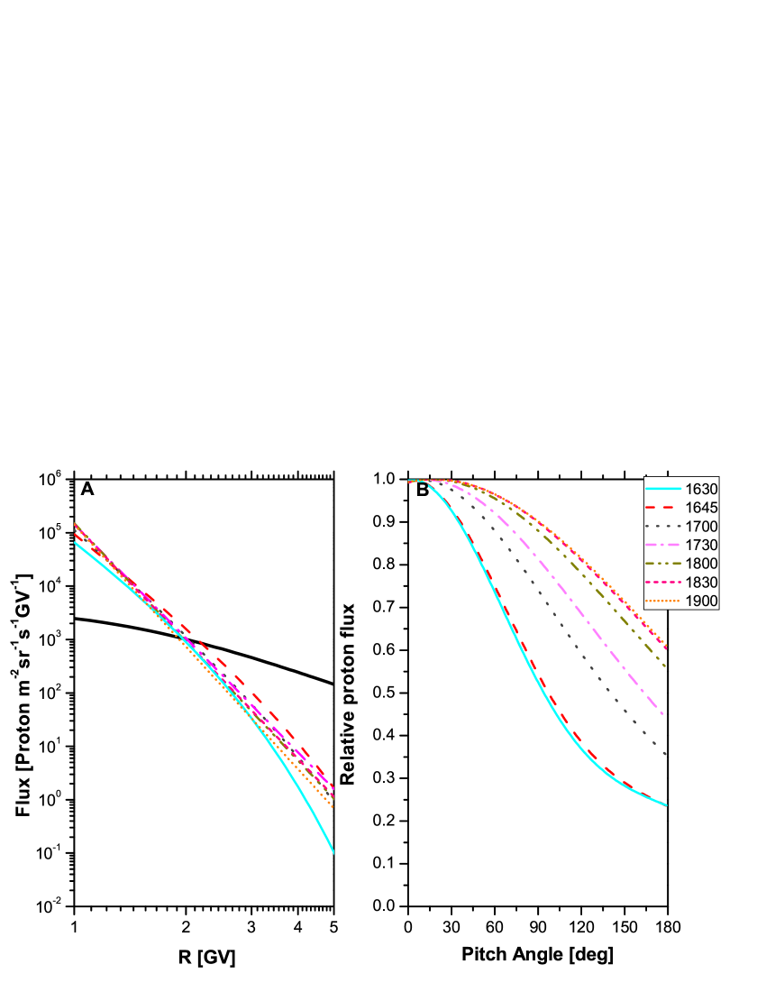
Figure 2: GLE particles rigidity spectra and PAD during GLE 72 on September 10, 2017, details are given in Table 1. Time (UT) corresponds to the start of the five minute interval over which the data are integrated. The black solid line of the left panel denotes the GCR particle flux computed on period corresponding to GLE 72 occurrence.

The rigidity spectrum and PAD are derived by minimizing the functional form $\mathcal{F}$ which is the sum of squared differences between the model $\frac{\Delta N_{i}}{N_{i}}_{mod.}$ and measured $\frac{\Delta N_{i}}{N_{i}}_{exp.}$ relative increases of NMs:

$$\mathcal{F}=\sum_{i=1}^{m}\left[\left(\frac{\Delta N_{i}}{N_{i}}\right)_{mod.}-\left(\frac{\Delta N_{i}}{N_{i}}\right)_{exp.}\right]^{2}$$ (3)

over $m$ NM stations, where $\Delta N_{i}$ and $N_{i}$ are the the count rate increase due to solar protons and the pre-event background counts due to GCRs of the $i$-th NM, respectively. Herein, the minimization of $\mathcal{F}$ is performed using a variable regularization similar to that proposed by Tikhonov et al. (1995) employing the Levenberg-Marquardt method (Levenberg, 1944; Marquardt, 1963). The goodness of the fit is based on residual $\mathcal{D}$ (Equation 4) (e.g. Himmelblau, 1972; Dennis and Schnabel, 1996).

$$\mathcal{D}=\frac{\sqrt{\sum_{i=1}^{m}\left[\left(\frac{\Delta N_{i}}{N_{i}}\right)_{mod.}-\left(\frac{\Delta N_{i}}{N_{i}}\right)_{meas.}\right]^{2}}}{\sum_{i=1}^{m}(\frac{\Delta N_{i}}{N_{i}})_{meas.}}$$ (4)

During the analysis, the background due to GCRs was averaged over two hours before the event’s onset, and the Forbush decrease started, on September 7, 2017, was explicitly considered in our analysis. Here we present the derived SEP characteristics, expanding the time interval reported in Mishev et al. (2018). The derived rigidity spectra of GLE particles were found to be relatively hard during the event onset (see Fig.2a) for a weak event and a softening of the spectra throughout the event was derived (e.g. Mishev et al., 2017, 2018). The derived spectral index after the event onset is in very good agreement with other estimates (e.g. Kataoka et al., 2018). After 17:15 UT the energy distribution of the GLE particles was described by a pure power-law rigidity spectrum. In addition, it was recently shown that this event was softer at high energies than average GLEs, but revealed hard spectrum at low energies (e.g. Cohen and Mewaldt, 2018). The angular distribution of the high energy solar particles broadened out throughout the event and was wide, except for the event onset (see Fig.2b). We assumed an isotropic SEP flux for conservative assessment of the exposure similarly to Copeland et al. (2008). The derived spectra and angular distributions will be integrated into the GLE database (Tuohino et al., 2018).

3 Assessment of effective dose rate at aviation altitudes during GLE 72

For the calculation of the effective dose rates during GLE 72 we employed a recently developed numerical model, which is based on pre-computed effective dose yield functions from high-statistics Monte Carlo simulations. These yield functions are the response of ambient air at a given altitude $h$ above sea level as the effective dose to a mono-energetic unit flux of primary CR particle entering the Earth’s atmosphere.

The effective dose rate at a given atmospheric altitude $h$ a.s.l. induced by primary CR particles is given by the expression:

$$E(h,T,\theta,\varphi)=\sum_{i}\int_{T_{cut,i}(P_{cut})}^{\infty}\int_{\Omega}J_{i}(T)Y_{i}(T,h)d\Omega(\theta,\varphi)dT,$$ (5)

where $P_{cut}$ is the local geomagnetic cut-off rigidity, $\Omega$ is a solid angle determined by the angles of incidence of the arriving particle $\theta$ (zenith) and $\varphi$ (azimuth), $J_{i}(T)$ is the differential energy spectrum of the primary CR at the top of the atmosphere for nuclei of type $i$ (proton or $\alpha-$particle) and $Y_{i}$ is the corresponding yield function. The integration is over the kinetic energy above $T_{cut,i}(P_{cut})$, which is defined by $P_{cut}$ for a nuclei of type $i$. The full description of the model with the corresponding look-up tables of the yield functions at several altitudes a.s.l. and comparison with reference data is given elsewhere (Mishev and Usoskin, 2015).

Here we computed the effective dose rate during GLE 72 using newly derived SEP spectra and angular distributions on the basis of NM data (details are given in Section 2) and Eq. 5. The exposure during GLE events is defined as a superposition of the GCRs and SEPs contributions. The radiation background due to GCR was computed by applying the force field model of galactic cosmic ray spectrum (Gleeson and Axford, 1968; Burger et al., 2000; Usoskin et al., 2005) with the corresponding parametrization of local interstellar spectrum (e.g. Usoskin et al., 2005; Usoskin and Kovaltsov, 2006), where the modulation potential is considered similar to Usoskin et al. (2011). For the computation of the exposure we do not consider the depression of GCRs due to the Forbush decrease, started on September 7, 2017. This results in a conservative approach for the contribution of GCRs to the exposure with eventual overestimation of the background exposure. Accordingly, the characteristics of energetic solar protons used in Eq. 5 were taken from Fig.1. The flux of incoming GLE particles was assumed to be isotropic, which is consistent with the derived angular distribution and allows one to assess conservatively the exposure (e.g. Copeland et al., 2008).

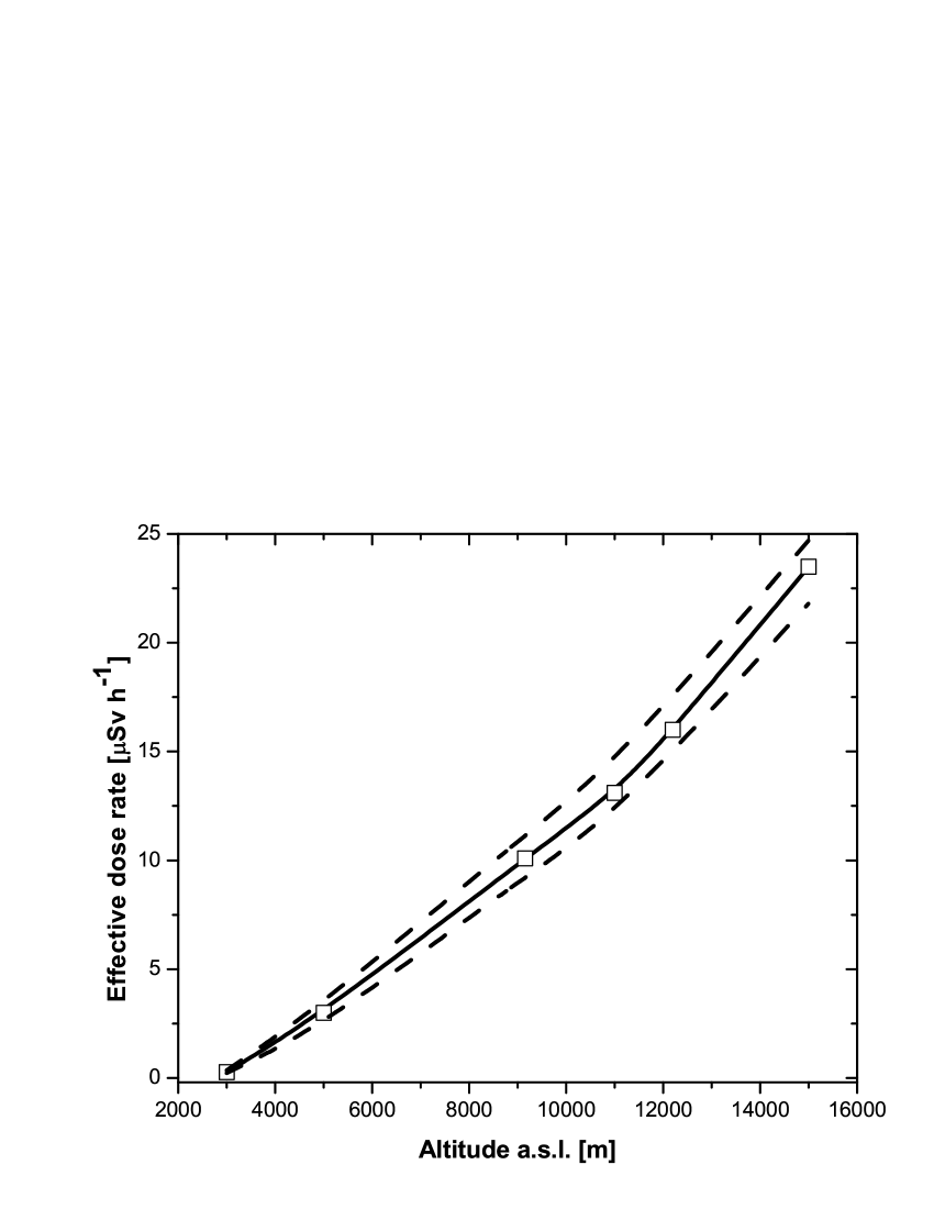
Figure 3: Computed maximal effective dose rate as a function of altitude a.s.l. during the main phase of GLE 72 on September 10, 2017. The dashed lines encompass the 95 $\%$ confidence interval

.

In this way we computed the effective dose rate during GLE 72 at several typical for cruise flight altitudes, namely 30 kft (9 100m), 35 kft (10 670m), 40 kft (12 200m) and 50 kft (15 200m) a.s.l.. The effective dose rate was estimated also at high-mountain altitude of about 3000 and 5000 m a.s.l. using the yield functions by Mishev (2016). These computations were performed for a high-latitude region with a low cut-off rigidity $P_{cut}$ $<$ 1 GV, where the expected exposure is maximal. Results during period with maximum exposure are presented in Fig. 3. The time evolution of the exposure throughout the event is computed at several altitudes.

One can see that the contribution of SEPs to the total exposure is comparable to the contribution due to GCRs, except for low altitudes. At the ground level, the contribution of SEPs to the total exposure is small, because of their considerably softer spectrum, compared to GCRs. The peak exposure is in the range of 20–24 $\mu$Sv.h^-1 at altitude of 50 kft a.s.l., 11–13 $\mu$Sv.h^-1 at altitude of 35 kft a.s.l. and about 10 $\mu$Sv.h^-1 at altitude of 30 kft a.s.l., during the main phase of the event, i.e., between 17:00 and 18:30 UT. During the late phase of the event (after 21:00 UT), the exposure decreases to roughly 20 $\mu$Sv.h^-1, 12 $\mu$Sv.h^-1 and about 10 $\mu$Sv.h^-1 at altitudes of 50, 35 and 30 kft a.s.l., respectively. The contribution of solar protons to the exposure considerably decreases during the late phase of the event.

The distribution of the exposure over the globe is determined by the cut-off rigidity, which is computed here using a combination of Tsyganenko 1989 (external) (Tsyganenko, 1989) and IGRF (internal) (Langel, 1987) geomagnetic models. This combination allows one to compute straightforwardly the cut-off rigidity with a reasonable precision (Kudela and Usoskin, 2004; Kudela et al., 2008; Nevalainen et al., 2013). An example of the distribution of the exposure as a function of the geographic coordinates for altitude of 50 kft a.s.l. during the main phase of GLE 72 is given in Fig. 4. The distribution of the effective dose rate reveals a maximum at polar and sub-polar regions and rapidly decreases at regions with higher cut-off rigidity. Similar computations were performed for lower cruise flight altitudes, the results are presented in Fig. 5 (35 kft a.s.l.) and Fig. 6 (30 kft a.s.l.). Computations for the late phase of the event depict similar distributions of the exposure, but with lower values. Those results are valid for the polar regions, while at low latitudes there is no notable change of the expected exposure, which is due to GCRs. Moreover, even a slight increase of the exposure at low latitudes is expected, because of the recovery of the Forbush decrease, but not considered here.

The exposure decreases significantly as a function of increasing cut-off rigidity. Below 30 kft, as well as at regions with $P_{cut}$ $\geq$ 2 GV, the contribution of SEPs becomes small even negligible, because their spectrum is considerably softer than the GCR spectrum.

The computed distributions of effective dose rates allow one to estimate the exposure of a crew members/passengers on board of a transcontinental flight during the GLE 72. Here we consider nearly a worst-case scenario, i.e., a polar route, departure time close to the event onset, high constant cruise altitude of 40 kft and a conservative approach for the exposure by assuming an isotropic SEP flux, without considering the effect of the Forbush decrease. Therefore, we present a very conservative assessment of the received effective dose by crew members/passengers during the GLE 72.

As an example, a crew members/passengers, would receive about 90 $\mu$Sv on a flight from Helsinki (HEL), Finland to Osaka (KIX), Japan (departure time 17:10 UT, 9h 30m duration, altitude 40 kft), 110 $\mu$Sv from Helsinki to New York–JFK (departure time 15:20 UT, 8h 40m duration, altitude 40 kft), respectively. Here, We do not consider change of the flight altitude during the ascending and the landing phase in order to conservatively assess the exposure. In both cases, the flight routes are along the great circle. Despite the shorter HEL–JFK flight, one would receive larger exposure, mostly because of the polar route. In addition, the HEL–JFK flight is during the main phase of the event, while HEL–KIX flight is during the main and late phase of the event, because of the later departure, according the actual flight information.

These results related to radiation environment during GLE 72 are compared with other similar estimates (e.g. Copeland et al., 2018; Kataoka et al., 2018; Matthiä et al., 2018). A good agreement, in the order of 10–14 $\%$, at altitude of 50 kft with the exposure reported by Copeland et al. (2018) is achieved. At lower levels the difference increases to 40–55 $\%$ at altitude of 40 kft and to 75 $\%$ at altitude of 35 kft, respectively. In all cases our model reveals greater exposure. The differences are consistent with recent reports (e.g. Bütikofer and Flückiger, 2013, 2015). They are most likely due to the slightly different SEP spectra derived using NM data (our analysis), compared to GOES data analysis (e.g. Copeland et al., 2018).

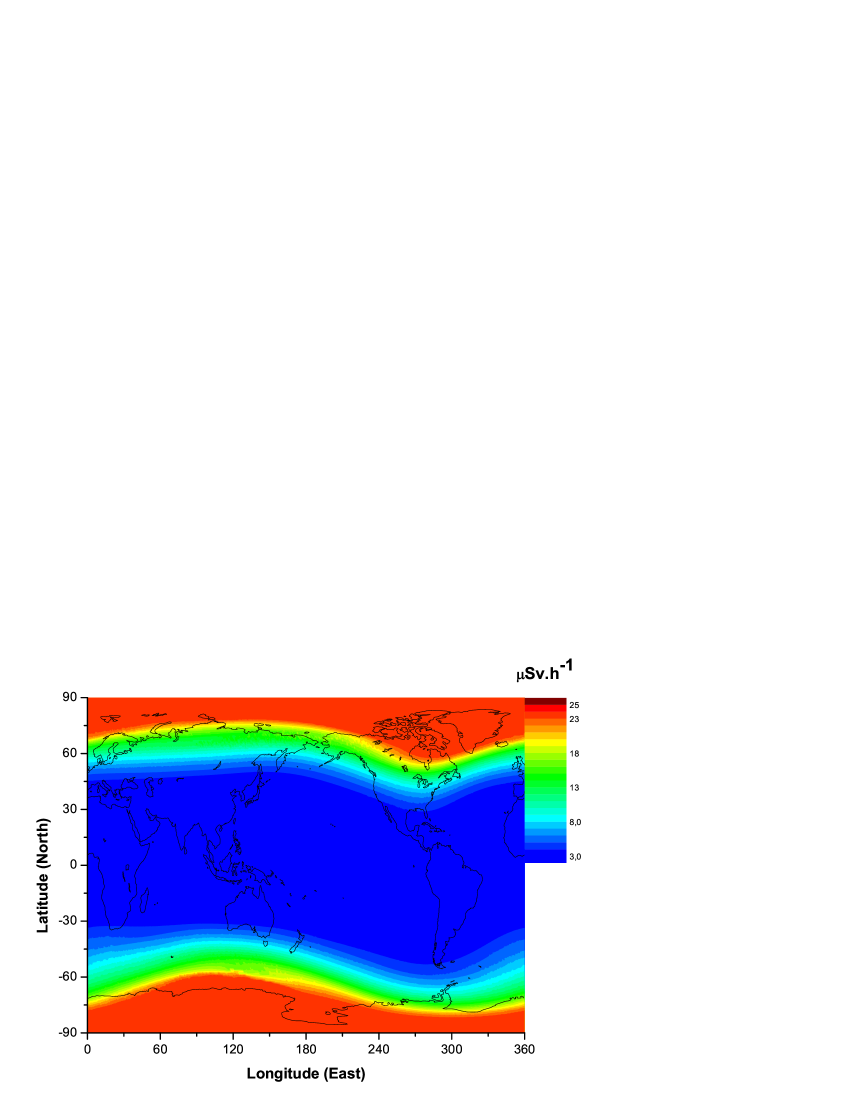
Figure 4: Distribution of the effective dose rate as a function of the geographic coordinates at altitude of 50 kft due to high energy GLE and GCR particles during the main phase of GLE 72 on September 10, 2017.

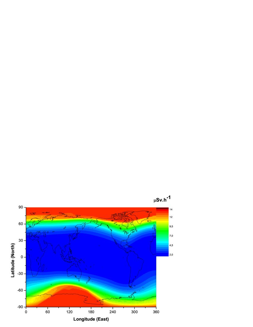
Figure 5: Distribution of the effective dose rate as a function of the geographic coordinates at altitude of 35 kft due to high energy GLE and GCR particles during the main phase of GLE 72 on September 10, 2017.

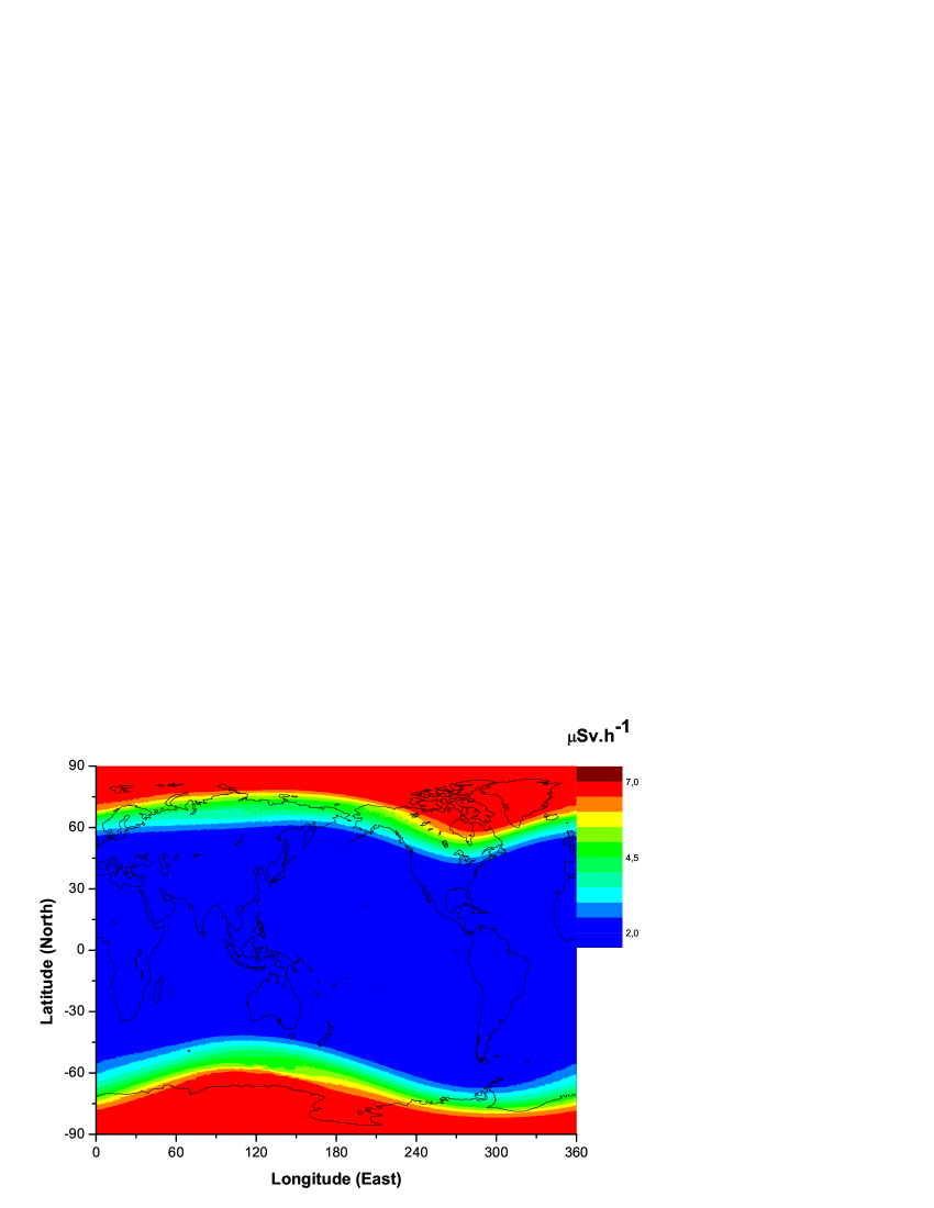
Figure 6: Distribution of the effective dose rate as a function of the geographic coordinates at altitude of 30 kft due to high energy GLE and GCR particles during the main phase of GLE 72 on September 10, 2017.

4 Summary and Discussion

In this study we presented reconstruction of rigidity spectrum and PAD of solar energetic protons during the GLE 72 using data from the global neutron monitor network. Using the reconstructed spectrum we assessed the exposure for crew members/passengers at several typical cruise flight altitudes in a polar region, assuming a conservative isotropic approach of the GLE particles angular distribution. We also conservatively calculated the received doses for two typical intercontinental flights: HEL– KIX (departure time 17:10 UT, 9h 30m duration, altitude 40 kft) and HEL–JFK (departure time 15:20 UT, 8h 40m duration, altitude 40 kft). We conclude that during a weak GLE event such as GLE 72 on September 10, 2017, the upper limit of the radiation exposure over a single flight is about 100 $\mu$Sv, with contribution of GCRs of about 60–65 $\mu$Sv, does not represent an important space weather issue. Usually, the pilots receive annually more than the annual general public limit of 1 mSv (e.g. EURATOM, 2014), with the majority receiving around 3 mSv (e.g. Bennett et al., 2013). However, the exposure during GLEs should be monitored. The presented results can be compared with other similar estimates.

The exposure at cruise flight altitudes during strong SEP events can be significantly enhanced compared to quiet periods. It is a superposition of contributions of GCRs and SEPs. As a result, during strong SEP events and GLEs, crew members/passengers may receive doses well above the background level due to GCRs (e.g. Matthiä et al., 2009; Tuohino et al., 2018). While the background exposure due to GCRs can be assessed by computations and/or on the basis of appropriate measurements, the estimation of the exposure due to high energy SEPs is rather complicated and it is performed retrospectively. Occurring sporadically, GLEs differ from each other in spectra and duration, and are therefore usually studied case by case. Deep and systematic study of the exposure during GLEs provides a good basis for further assessment of space weather effects related to accumulated doses at aviation flight altitudes and allows one to compare and adjust possible uncertainties in the existing methods and models in this field.

References

- Asorey et al. (2018) Asorey, H., L. Núñez, and M. Suárez-Durán (2018), Preliminary results from the latin american giant observatory space weather simulation chain, Space Weather, 16(5), 461–475, doi:10.1002/2017SW001774.
- Baker (1998) Baker, D. (1998), What is space weather?, Advances in Space Research, 22(1), 7–16.
- Bazilevskaya et al. (2008) Bazilevskaya, G. A., I. G. Usoskin, E. Flückiger, R. Harrison, L. Desorgher, B. Bütikofer, M. Krainev, V. Makhmutov, Y. Stozhkov, A. Svirzhevskaya, N. Svirzhevsky, and G. Kovaltsov (2008), Cosmic ray induced ion production in the atmosphere, Space Science Reviews, 137, 149–173.
- Bennett et al. (2013) Bennett, L., B. Lewis, B. Bennett, M. McCall, M. Bean, L. Doré, and I. Getley (2013), A survey of the cosmic radiation exposure of air canada pilots during maximum galactic radiation conditions in 2009, Radiation Measurements, 49(1), 103–108, doi:10.1016/j.radmeas.2012.12.004.
- Burger et al. (2000) Burger, R., M. Potgieter, and B. Heber (2000), Rigidity dependence of cosmic ray proton latitudinal gradients measured by the ulysses spacecraft: Implication for the diffusion tensor, Journal of Geophysical Research, 105, 27 447–27 445.
- Bütikofer and Flückiger (2013) Bütikofer, R., and E. Flückiger (2013), Differences in published characteristics of GLE 60 and their consequences on computed radiation dose rates along selected flight paths, Journal of Physics: Conference Series, 409(1), 012,166.
- Bütikofer and Flückiger (2015) Bütikofer, R., and E. Flückiger (2015), What are the causes for the spread of GLE parameters deduced from nm data?, Journal of Physics: Conference Series, 632(1), doi:10.1088/1742-6596/632/1/012053.
- Cohen and Mewaldt (2018) Cohen, C. M. S., and R.A. Mewaldt (2018), The ground‐level enhancement event of September 2017 and other large solar energetic particle events of cycle 24, Space Weather, 16, doi:10.1029/2018SW002006.
- Copeland et al. (2008) Copeland, K., H. Sauer, F. Duke, and W. Friedberg (2008), Cosmic radiation exposure of aircraft occupants on simulated high-latitude flights during solar proton events from 1 January 1986 through 1 January 2008, Advances in Space Research, 42(6), 1008–1029.
- Copeland et al. (2018) Copeland, K., D. Matthiä, and M. Meier (2018), Solar cosmic ray dose rate assessments during GLE 72 using MIRA and PANDOCA, Space Weather, 16, doi:10.1029/2018SW001917.
- Cramp et al. (1997) Cramp, J., M. Duldig, E. Flückiger, J. Humble, M. Shea, and D. Smart (1997), The October 22, 1989,solar cosmic enhancement: ray an analysis the anisotropy spectral characteristics, Journal of Geophysical Research, 102(A11), 24 237–24 248.
- Dennis and Schnabel (1996) Dennis, J., and R. Schnabel (1996), Numerical Methods for Unconstrained Optimization and Nonlinear Equations, Prentice-Hall, Englewood Cliffs.
- EURATOM (2014) EURATOM (2014), Directive 2013/59/Euratom of 5 December 2013 laying down basic safety standards for protection against the dangers arising from exposure to ionising radiation, and repealing directives 89/618/Euratom, 90/641/Euratom, 96/29/Euratom, 97/43/Euratom and 2003/122/Euratom., Official Journal of the European Communities, 57(L13).
- Gil et al. (2015) Gil, A., I. Usoskin, G. Kovaltsov, A. Mishev, C. Corti, and V. Bindi (2015), Can we properly model the neutronmonitor count rate?, J. Geophys. Res., 120, 7172–7178.
- Gleeson and Axford (1968) Gleeson, L., and W. Axford (1968), Solar modulation of galactic cosmic rays, Astrophysical Journal, 154, 1011–1026.
- Gopalswamy et al. (2012) Gopalswamy, N., H. Xie, S. Yashiro, S. Akiyama, P. Mäkelä, and I. Usoskin (2012), Properties of ground level enhancement events and the associated solar eruptions during solar cycle 23, Space Science Reviews, 171(1-4), 23–60.
- Himmelblau (1972) Himmelblau, D. (1972), Applied Nonlinear Programming, Mcgraw-Hill(Tx).
- ICRP (2007) ICRP (2007), ICRP publication 103: The 2007 recommendations of the international commission on radiological protection., Annals of the ICRP, 37(2-4).
- Kataoka et al. (2018) Kataoka, R., T. Sato, S. Miyake, D. Shiota, and Y. kubo (2018), Radiation Dose Nowcast for the Ground Level Enhancement on 10–11 September 2017, Space Weather, 16, doi:10.1029/2018SW001874.
- Kudela and Usoskin (2004) Kudela, K., and I. Usoskin (2004), On magnetospheric transmissivity of cosmic rays, Czechoslovak Journal of Physics, 54(2), 239–254.
- Kudela et al. (2008) Kudela, K., R. Bučik, and P. Bobik (2008), On transmissivity of low energy cosmic rays in disturbed magnetosphere, Advances in Space Research, 42(7), 1300–1306.
- Kuwabara et al. (2006) Kuwabara, T., J. Bieber, J. Clem, P. Evenson, and R. Pyle (2006), Development of a ground level enhancement alarm system based upon neutron monitors, Space Weather, 4(10), S10,001, doi:10.1029/2006SW000223.
- Langel (1987) Langel, R. (1987), Main field in geomagnetism, in Geomagnetism, chap. 1, pp. 249–512, J.A. Jacobs Academic Press, London.
- Latocha et al. (2009) Latocha, M., P. Beck, and S. Rollet (2009), Avidos-a software package for european accredited aviation dosimetry, Radiation Protection Dosimetry, 136(4), 286–290, doi:10.1093/rpd/ncp126.
- Levenberg (1944) Levenberg, K. (1944), A method for the solution of certain non-linear problems in least squares, Quarterly of Applied Mathematics, 2, 164–168.
- Lilensten and Bornarel (2009) Lilensten, L., and J. Bornarel (2009), Space Weather, Environment and Societies, Springer, Dordrecht.
- Mangeard et al. (2016) Mangeard, P.-S., D. Ruffolo, A. Sáiz, W. Nuntiyakul, J. Bieber, J. Clem, P. Evenson, R. Pyle, M. Duldig, and J. Humble (2016), Dependence of the neutron monitor count rate and time delay distribution on the rigidity spectrum of primary cosmic rays, Journal of Geophysical Research: Space Physics, 121(12), 11 620–11 636, doi:10.1002/2016JA023515.
- Marquardt (1963) Marquardt, D. (1963), An algorithm for least-squares estimation of nonlinear parameters, SIAM Journal on Applied Mathematics, 11(2), 431–441.
- Matthiä et al. (2009) Matthiä, D., B. Heber, G. Reitz, L. Sihver, T. Berger, and M. Meier (2009), The ground level event 70 on december 13th, 2006 and related effective doses at aviation altitudes, Radiation Protection Dosimetry, 136(4), 304–310.
- Matthiä et al. (2018) Matthiä, D., M. Meier, and T. Berger (2018), The solar particle event on 10-13 September 2017 – spectral reconstruction and calculation of the radiation exposure in aviation and space, Space Weather, 16, doi:10.1029/2018SW001921.
- Meier et al. (2018) Meier, M.M., K. Copeland, D. Matthiä, C.J. Mertens and K. Schennetten (2018), First steps toward the verification of models for the assessment of the radiation exposure at aviation altitudes during quiet space weather conditions, Space Weather, 16(9), 1269–1276 doi:10.1029/2018SW001984.
- Menzel (2010) Menzel, H. (2010), The international commission on radiation units and measurements, Journal of the ICRU, 10(2), 1–35.
- Mertens (2016) Mertens, C.(2016), Overview of the Radiation Dosimetry Experiment (RaD-X) flight mission, Space Weather, 14(11), 921–934.
- Mertens et al. (2013) Mertens, C., M. Meier, S. Brown, R. Norman, and X. Xu (2013), Nairas aircraft radiation model development, dose climatology, and initial validation, Space Weather, 11(10), 603–635.
- Mishev (2016) Mishev, A. (2016), Contribution of cosmic ray particles to radiation environment at high mountain altitude: Comparison of Monte Carlo simulations with experimental data, Journal of Environmental Radioactivity, 153, 15–22, doi:10.1016/j.jenvrad.2015.12.002.
- Mishev and Usoskin (2015) Mishev, A., and I. Usoskin (2015), Numerical model for computation of effective and ambient dose equivalent at flight altitudes: Application for dose assessment during GLEs, Journal of Space Weather and Space Climate, 5(3), A10, doi:10.1051/swsc/2015011.
- Mishev and Usoskin (2016) Mishev, A., and I. Usoskin (2016), Analysis of the ground level enhancements on 14 July 2000 and on 13 December 2006 using neutron monitor data, Solar Physics, 291(4), 1225–1239.
- Mishev et al. (2013) Mishev, A., I. Usoskin, and G. Kovaltsov (2013), Neutron monitor yield function: New improved computations, Journal of Geophysical Research, 118, 2783–2788.
- Mishev et al. (2014) Mishev, A., L. Kocharov, and I. Usoskin (2014), Analysis of the ground level enhancement on 17 May 2012 using data from the global neutron monitor network, Journal of Geophysical Research, 119, 670–679.
- Mishev et al. (2017) Mishev, A., S. Poluianov, and S. Usoskin (2017), Assessment of spectral and angular characteristics of sub-GLE events using the global neutron monitor network, Journal of Space Weather and Space Climate, 7, A28, doi:10.1051/swsc/2017026.
- Mishev et al. (2018) Mishev, A., I. Usoskin, O. Raukunen, M. Paassilta, E. Valtonen, L. Kocharov, and R. Vainio (2018), First analysis of GLE 72 event on 10 september 2017: Spectral and anisotropy characteristics, Solar Physics, 293, 136, doi:10.1007/s11207-018-1354-x.
- Moraal and McCracken (2012) Moraal, H., and K. McCracken (2012), The time structure of ground level enhancements in solar cycle 23, Space Science Reviews, 171(1-4), 85–95.
- Nevalainen et al. (2013) Nevalainen, J., I. Usoskin, and A. Mishev (2013), Eccentric dipole approximation of the geomagnetic field: Application to cosmic ray computations, Advances in Space Research, 52(1), 22–29.
- Sato et al. (2018) Sato, T., R. Kataoka, D. Shiota, Y. Kubo, M. Ishii, H. Yasuda, S. Miyake, I. Park, and Y. Miyoshi (2018), Real time and automatic analysis program for wasavies: Warning system for aviation exposure to solar energetic particles, Space Weather, 16(7), 924–936, doi:10.1029/2018SW001873.
- Shea and Smart (1982) Shea, M., and D. Smart (1982), Possible evidence for a rigidity-dependent release of relativistic protons from the solar corona, Space Science Reviews, 32, 251–271.
- Shea and Smart (2000) Shea, M., and D. Smart (2000), Cosmic ray implications for human health, Space Science Reviews, 93(1-2), 187–205.
- Spurny et al. (1996) Spurny, F., I.Votockova, and J. Bottollier-Depois (1996), Geographical influence on the radiation exposure of an aircrew on board a subsonic aircraft, Radioprotection, 31(2), 275–280.
- Spurny et al. (2002) Spurny, F., T.Dachev, and K. Kudela (2002), Increase of onboard aircraft exposure level during a solar flare, Nuclear Energy Safety, 10(48), 396–400.
- Tikhonov et al. (1995) Tikhonov, A., A. Goncharsky, V. Stepanov, and A. Yagola (1995), Numerical Methods for Solving ill-Posed Problems, Kluwer Academic Publishers, Dordrecht.
- Tobiska et al. (2018) Tobiska, W.K., L. Didkovsky, K. Judge, S. Weimna, D. Bouwer, J. Bailey, et. al., (2018), Analytical representations for characterizing the global aviation radiation environment based on model and measurement databases, Space Weather, 16, doi:10.1029/2018SW001843
- Tsyganenko (1989) Tsyganenko, N. (1989), A magnetospheric magnetic field model with a warped tail current sheet, Planetary and Space Science, 37(1), 5–20.
- Tuohino et al. (2018) Tuohino, S., A. Ibragimov, I. Usoskin, and A. Mishev (2018), Upgrade of gle database: Assessment of effective dose rate at flight altitude, Advances in Space Research, 62(2), 398–407, doi:10.1016/j.asr.2018.04.021.
- Usoskin and Kovaltsov (2006) Usoskin, I., and G. Kovaltsov (2006), Cosmic ray induced ionization in the atmosphere: Full modeling and practical applications, Journal of Geophysical Research, 111, D21206.
- Usoskin et al. (2005) Usoskin, I., K. Alanko-Huotari, G. Kovaltsov, and K. Mursula (2005), Heliospheric modulation of cosmic rays: Monthly reconstruction for 1951-2004,, J. Geophys. Res., 110, A12108.
- Usoskin et al. (2011) Usoskin, I., G. Bazilevskaya, and G. Kovaltsov (2011), Solar modulation parameter for cosmic rays since 1936 reconstructed from ground-based neutron monitors and ionization chambers, Journal of Geophysical Research, 116, A02,104.
- Vainio et al. (2009) Vainio, R., L. Desorgher, D. Heynderickx, M. Storini, E. Flückiger, R. Horne, G. Kovaltsov, K. Kudela, M. Laurenza, S. McKenna-Lawlor, H. Rothkaehl, and I. Usoskin (2009), Dynamics of the earth’s particle radiation environment, Space Science Reviews, 147(3-4), 187–231.
- Vashenyuk et al. (2008) Vashenyuk, E., Y. Balabin, B. Gvozdevsky, and L. Schur (2008), Characteristics of relativistic solar cosmic rays during the event of december 13, 2006, Geomagnetism and Aeronomy, 48(2), 149–153.