Extensivity, entropy current, area law and Unruh effect

Abstract

We present a general method to determine the entropy current of relativistic matter at local thermodynamic equilibrium in quantum statistical mechanics. Provided that the local equilibrium operator is bounded from below and its lowest lying eigenvector is non-degenerate, it is proved that, in general, the logarithm of the partition function is extensive, meaning that it can be expressed as the integral over a 3D space-like hypersurface of a vector current, and that an entropy current exists. We work out a specific calculation for a non-trivial case of global thermodynamic equilibrium, namely a system with constant comoving acceleration, whose limiting temperature is the Unruh temperature. We show that the integral of the entropy current in the right Rindler wedge is the entanglement entropy.

I Introduction

In recent years there has been a considerable interest on the foundations of relativistic hydrodynamics. One of the key quantities is the so-called entropy current $s^{\mu}$, which is one of the postulated ingredients of Israel’s formulation israel . Therein, entropy current plays a very important role because, as its divergence ought to be positive, its form entails the constitutive equations of the conserved currents (stress-energy tensor, charged currents) as a function of the gradients of the intensive thermodynamic parameters. Over the last decade, there has been a very large number of studies where the structure of the entropy current in relativistic hydrodynamics was involved, whose a small sample is reported in the bibliography list1 ; list2 ; list3 ; list4 ; list5 ; haehl1 ; list6 ; list7 . On the other hand, there have been attempts kaminski to formulate relativistic hydrodynamics without an entropy current.

In most of these studies, the structure of the entropy current is postulated based on some classical form of the thermodynamics laws supplemented by more elaborate methods to include dissipative corrections sayantani1 ; sayantani2 , but, strictly speaking, it is not derived. The ultimate reason for the apparent insufficient definition is that the entropy current, unlike the stress-energy tensor or charged currents, in the familiar Quantum Field Theory, is not the mean value of a local operator built with quantum fields (in the generating functional approach, this difference can be rephrased by saying that the entropy current cannot be obtained by taking functional derivatives with respect to some external source). Another reason for this indeterminacy is the fact that, while in quantum statistical mechanics the total entropy has a precise definition in terms of the density operator (von Neumann formula) $S=-{\rm tr}({\widehat{\rho}}\log{\widehat{\rho}})$, the entropy current, which should be a more fundamental quantity than the total entropy in a general relativistic framework, has not.

In this work, we will show that it is indeed possible to provide a rigorous definition of the entropy current in quantum relativistic statistical mechanics and thereby to derive its form in a situation of local thermodynamic equilibrium, which is the underlying assumption of relativistic hydrodynamics. The method is based on the definition of a density operator at local thermodynamic equilibrium put forward in the late ’70s by Zubarev and van Weert zubarev ; weert and reworked more recently in refs. becalocal ; hongo . The key step to show that an entropy current exists is the proof that, in a relativistic theory, the logarithm of the partition function is extensive, i.e. it can be expressed as an integral over a 3D space-like hypersurface of a four-vector field. We will provide, to the best of our knowledge, the first general proof of this usually tacitly understood hypothesis under very general conditions.

After the general method, we will present a specific, non-trivial instance of calculation of the entropy current which is especially interesting for it is related to the Unruh effect. Indeed, we will show that in the Minkowski vacuum an acceleration involves a non-vanishing finite entropy current in some region which, once integrated, gives rise to its total entanglement entropy.

Notation

In this paper we adopt the natural units, with $\hbar=c=K=1$. The Minkowskian metric tensor is $g={\rm diag}(1,-1,-1,-1)$ and for the Levi-Civita symbol we use the convention $\varepsilon^{0123}=1$. Operators in Hilbert space will be denoted by an upper hat, e.g. $\widehat{\sf R}$.
We will use the relativistic notation with repeated indices assumed to be saturated, and contractions of indices will be sometimes denoted with dots, e.g. $b\cdot\widehat{P}=b_{\mu}\widehat{P}^{\mu}$ or $\varpi:\widehat{J}=\varpi_{\mu\nu}\widehat{J}^{\mu\nu}$.
$\nabla_{\mu}$ denotes covariant derivative in curved space-time.

II Extensivity and entropy current

In quantum statistical mechanics, the state of a physical system is described by a density operator ${\widehat{\rho}}$. At global thermodynamic equilibrium, $\widehat{\rho}$ is determined, according to the maximum entropy principle, by maximizing the entropy $S=-{\rm tr}(\widehat{\rho}\log\widehat{\rho})$ with a set of constraints; for instance fixing the value of the energy and some possible charges. Similarly, in a situation of local thermodynamic equilibrium (LTE), the density operator $\widehat{\rho}_{\rm LE}$ is determined by maximizing the entropy constrained with energy-momentum and charge densities. In a relativistic framework, the LTE density operator definition depends on a 3D space-like hypersurface $\Sigma$ where the densities are given; the fully covariant expression reads zubarev :

$$\widehat{\rho}_{\rm LE}=\frac{1}{Z_{\rm LE}}\exp\left[-\int_{\Sigma}{\rm d}\Sigma_{\mu}\left(\widehat{T}^{\mu\nu}\beta_{\nu}-\zeta\widehat{j}^{\mu}\right)\right]$$ (1)

where:

$$Z_{\rm LE}={\rm tr}\left(\exp\left[-\int_{\Sigma}{\rm d}\Sigma_{\mu}\left(\widehat{T}^{\mu\nu}\beta_{\nu}-\zeta\widehat{j}^{\mu}\right)\right]\right)$$

is the partition function. In the eq. (1), $\widehat{T}^{\mu\nu}$ is the stress-energy tensor, $\widehat{j}^{\mu}$ is a conserved current , $\beta_{\nu}$ is the time-like four-temperature vector, whose magnitude is the inverse comoving temperature:

$$T=\frac{1}{\sqrt{\beta^{2}}}$$ (2)

while its direction defines a flow velocity becalocal :

$$u^{\mu}=\frac{\beta^{\mu}}{\sqrt{\beta^{2}}},$$ (3)

and $\zeta$ is a scalar whose meaning is the ratio between comoving chemical potential and comoving temperature, i.e:

$$\zeta=\frac{\mu}{T}$$

With the density operator (1), one can calculate the total entropy as a function of the four-temperature, which turns out to be:

$$S=\log Z_{\rm LE}+\int_{\Sigma}{\rm d}\Sigma_{\mu}\left(\langle\widehat{T}^{\mu\nu}\rangle_{\rm LE}\beta_{\nu}-\zeta\langle\widehat{j}^{\mu}\rangle_{\rm LE}\right),$$ (4)

where by $\langle\;\rangle_{\rm LE}$ we mean the expectation value calculated with $\widehat{\rho}_{\rm LE}$. The expectation value of a local operator ${\widehat{O}}(x)$ is then a local intensive quantity depending only on $x$ provided that $x$ belongs to the hypersurface $\Sigma$ in the definition of the operator (1). Particularly, if $\Sigma$ is a hyperplane $t=const$, this means that the time component $x^{0}$ of $x$ must be equal to $t$. This condition will be henceforth understood. For an entropy current to exist, meaning that:

$$S=\int_{\Sigma}{\rm d}\Sigma_{\mu}\,s^{\mu},$$ (5)

it can be readily seen from eq. (4) that $\log Z_{\rm LE}$ must be extensive, namely that there must be a four-vector $\phi$, called thermodynamic potential current, such that:

$$\log Z_{\rm LE}=\int_{\Sigma}{\rm d}\Sigma_{\mu}\,\phi^{\mu}$$

so that, comparing eqs. (4) and (5),

$$s^{\mu}=\phi^{\mu}+\langle\widehat{T}^{\mu\nu}\rangle_{\rm LE}\beta_{\nu}-\zeta\langle\widehat{j}^{\mu}\rangle_{\rm LE}.$$

Notice that both $\phi$ and $s$ are defined up to an arbitrary four-vector tangent to the space-like hypersurface $\Sigma$.

The existence of the thermodynamic potential current and, as a consequence, of the entropy current, is usually assumed. One of the goals of this work is to show that its existence can be proved under very general hypotheses. To begin with, let us modify the LTE density operator introducing a dimensionless parameter $\lambda$:

$$\widehat{\rho}_{\rm LE}(\lambda)=\frac{1}{Z_{\rm LE}(\lambda)}\exp\left[-\lambda\int_{\Sigma}{\rm d}\Sigma_{\mu}\left(\widehat{T}^{\mu\nu}\beta_{\nu}-\zeta\widehat{j}^{\mu}\right)\right]$$ (6)

so that for $\lambda=1$ we recover the actual LTE density operator. Since:

$$Z_{\rm LE}(\lambda)={\rm tr}\left(\exp\left[-\lambda\int_{\Sigma}{\rm d}\Sigma_{\mu}\left(\widehat{T}^{\mu\nu}\,\beta_{\nu}-\zeta\widehat{j}^{\mu}\right)\right]\right),$$

by taking the derivative of the trace, we come to:

$$\frac{\partial\log Z_{\rm LE}(\lambda)}{\partial\lambda}=-\int_{\Sigma}{\rm d}\Sigma_{\mu}\left(\langle\widehat{T}^{\mu\nu}\rangle_{\rm LE}(\lambda)\,\beta_{\nu}-\zeta\langle\widehat{j}^{\mu}\rangle_{\rm LE}(\lambda)\right),$$

and, by integrating both sides:

$$\log Z_{\rm LE}-\log Z_{\rm LE}(\lambda_{0})=-\int_{\lambda_{0}}^{1}{\rm d}\lambda\int_{\Sigma}{\rm d}\Sigma_{\mu}\left(\langle\widehat{T}^{\mu\nu}\rangle_{\rm LE}(\lambda)\,\beta_{\nu}-\zeta\langle\widehat{j}^{\mu}\rangle_{\rm LE}(\lambda)\right)$$ (7)

for some $\lambda_{0}$, being $\log Z_{\rm LE}(1)$ the actual $\log Z_{\rm LE}$. If we can now exchange the integrations in eq. (7), we get:

$$\log Z_{\rm LE}-\log Z_{\rm LE}(\lambda_{0})=-\int_{\Sigma}{\rm d}\Sigma_{\mu}\,\int_{\lambda_{0}}^{1}{\rm d}\lambda\left(\langle\widehat{T}^{\mu\nu}\rangle_{\rm LE}(\lambda)\,\beta_{\nu}-\zeta\langle\widehat{j}^{\mu}\rangle_{\rm LE}(\lambda)\right).$$

Thus, if there exists a particular $\lambda_{0}$ such that $\log Z_{{\rm LE}}(\lambda_{0})=0$, it is proved that $\log Z_{\rm LE}$ is extensive and, at the same time, we have a method to determine the thermodynamic potential current:

$$\log Z_{\rm LE}=\int_{\Sigma}{\rm d}\Sigma_{\mu}\,\phi^{\mu},\qquad\phi^{\mu}=-\int_{\lambda_{0}}^{1}{\rm d}\lambda\left(\langle\widehat{T}^{\mu\nu}\rangle_{\rm LE}(\lambda)\,\beta_{\nu}-\zeta\langle\widehat{j}^{\mu}\rangle_{\rm LE}(\lambda)\right).$$

At a glance, one would say that $\lambda=+\infty$ can make $Z_{\rm LE}(\lambda)$ very small. More thoroughly, one should study the spectrum of the local equilibrium operator in the exponent of eq. (1), defined as:

$${\widehat{\Upsilon}}\equiv\int_{\Sigma}{\rm d}\Sigma_{\mu}\left(\widehat{T}^{\mu\nu}\beta_{\nu}-\zeta\widehat{j}^{\mu}\right).$$ (8)

It is easily realized that this operator, if $\zeta=0$, is but the Hamiltonian divided by the temperature in the special case where $\beta=1/T(1,{\bf 0})$. Suppose that the local equilibrium operator ${\widehat{\Upsilon}}$ is bounded from below, i.e. there exists a minimum eigenvalue $\Upsilon_{0}$ with a corresponding eigenvector $|0\rangle$, which is supposedly non-degenerate. In this case, ordering the eigenvalues $\Upsilon_{0}<\Upsilon_{1}<\Upsilon_{2}\ldots$, and if the lowest eigenvector is non-degenerate the trace can be written as:

$$Z_{\rm LE}(\lambda)={\rm tr}\left({\rm e}^{-\lambda{\widehat{\Upsilon}}}\right)={\rm e}^{-\lambda\Upsilon_{0}}\left(1-{\rm e}^{-\lambda(\Upsilon_{1}-\Upsilon_{0})}-{\rm e}^{-\lambda(\Upsilon_{2}-\Upsilon_{0})}-\cdots\right),$$

so, if $\Upsilon_{0}=0$ and we let $\lambda\to+\infty$, we obtain the sought solution, that is:

$$\lim_{\lambda\to+\infty}Z_{\rm LE}(\lambda)=1\qquad\implies\qquad\lim_{\lambda\to+\infty}\log Z_{\rm LE}(\lambda)=0.$$

One can now take advantage of the invariance of the density operator (1) by subtraction of a constant number in the exponent. What we mean is that ${\widehat{\rho}}$ is invariant, and entropy as well, if we replace ${\widehat{\Upsilon}}$ in eq. (8) with:

$$\begin{split}{\widehat{\Upsilon}}\mapsto{\widehat{\Upsilon}}-\Upsilon_{0}&={\widehat{\Upsilon}}-\langle 0|{\widehat{\Upsilon}}|0\rangle\\ &=\int_{\Sigma}{\rm d}\Sigma_{\mu}\left[\left(\widehat{T}^{\mu\nu}-\langle 0|\widehat{T}^{\mu\nu}|0\rangle\right)\beta_{\nu}-\zeta\left(\widehat{j}^{\mu}-\langle 0|\widehat{j}^{\mu}|0\rangle\right)\right]\end{split}$$

and calculate the partition function accordingly, that is $Z^{\prime}={\rm tr}(\exp[-{\widehat{\Upsilon}}+\Upsilon_{0}])$. Hence, the new $\lambda$-dependent partition function reads:

$$Z^{\prime}_{\rm LE}(\lambda)={\rm tr}\left(\exp\left\{-\lambda\int_{\Sigma}{\rm d}\Sigma_{\mu}\left[\left(\widehat{T}^{\mu\nu}-\langle 0|\widehat{T}^{\mu\nu}|0\rangle\right)\beta_{\nu}-\zeta\left(\widehat{j}^{\mu}-\langle 0|\widehat{j}^{\mu}|0\rangle\right)\right]\right\}\right)$$

We note in passing that the subtraction of the expectation value of ${\widehat{T}}^{\mu\nu}$ in the lowest lying eigenvector of ${\widehat{\Upsilon}}$ does not imply that the thereby obtained operator $\widehat{T}^{\mu\nu}-\langle 0|\widehat{T}^{\mu\nu}|0\rangle$ is the physically renormalized one. In fact, in the accelerated thermodynamic equilibrium case, the physical operator is obtained by subtracting the expectation value in the Minkowski vacuum becaunruh whereas the lowest lying eigenvector is the so-called Rindler vacuum, as we will see in Section IV.

The new partition function is such that $Z^{\prime}_{\rm LE}(\infty)=1$, and the thermodynamic potential current is thus given by

$$\phi^{\mu}=\int_{1}^{+\infty}{\rm d}\lambda\left[\left(\langle{\widehat{T}}^{\mu\nu}\rangle_{\rm LE}(\lambda)-\langle 0|{\widehat{T}}^{\mu\nu}|0\rangle\right)\beta_{\nu}-\zeta\left(\langle\widehat{j}^{\mu}\rangle_{\rm LE}(\lambda)-\langle 0|\widehat{j}^{\mu}|0\rangle\right)\right].$$ (9)

Consequently, the entropy current will be:

$$s^{\mu}=\phi^{\mu}+\left(\langle{\widehat{T}}^{\mu\nu}\rangle_{\rm LE}-\langle 0|{\widehat{T}}^{\mu\nu}|0\rangle\right)\beta_{\nu}-\zeta\left(\langle\widehat{j}^{\mu}\rangle_{\rm LE}-\langle 0|\widehat{j}^{\mu}|0\rangle\right).$$ (10)

These formulae show that the thermodynamic potential current is obtained by effectively integrating the temperature dependence of the currents, as $\lambda$ multiplies $\beta$ and $\zeta$. Even in the presence of first order phase transitions, with discontinuities in the mean values of stress-energy tensor and charged current as a function of the temperature, the integral is still feasible and makes perfect sense.

We can finally draw an important conclusions regarding the existence of the entropy current.

Theorem.

If the spectrum of the local equilibrium operator (8) is bounded from below, and if the eigenvector corresponding to its lowest eigenvalue is non-degenerate, the logarithm of the partition function is extensive. Thus, we can obtain a thermodynamic potential current by integrating the difference between the expectation value of the stress-energy tensor and of the conserved currents and their expectation value in the lowest lying eigenvector of the local equilibrium operator.

So, to solve the problem, one just needs to determine the mean values of the stress-energy tensor and of the currents. We will see how this can be accomplished in a non-trivial case in Section IV.

III Thermodynamic equilibrium with acceleration in Minkowski space-time

The local thermodynamic equilibrium density operator (1) can be promoted to global thermodynamic equilibrium when it becomes time-independent, or, in covariant language, independent of the space-like hypersurface $\Sigma$. This has been studied in detail elsewhere becacov . Global thermodynamic equilibrium occurs when $\zeta$ is constant and the four-temperature $\beta$ is a Killing vector, that is:

$$\nabla_{\mu}\beta_{\nu}+\nabla_{\nu}\beta_{\mu}=0.$$ (11)

It is readily seen from eqs. (9) and (10) that, in this case, if the stress-energy tensor and the currents are conserved, so are the thermodynamic potential current and the entropy current:

$$\nabla_{\mu}\phi^{\mu}=0,\qquad\nabla_{\mu}s^{\mu}=0$$

in agreement with the general condition that at global thermodynamic equilibrium the entropy production rate vanishes.

In Minkowski space-time the general solution of the Killing equation (11) is

$$\beta_{\mu}=b_{\mu}+\varpi_{\mu\nu}x^{\nu},$$ (12)

where $b$ is a constant four-vector and $\varpi$ a constant anti-symmetric tensor called thermal vorticity. The latter can be expressed as the exterior derivative of the four-temperature, i.e. $\varpi_{\mu\nu}=-\frac{1}{2}(\partial_{\mu}\beta_{\nu}-\partial_{\nu}\beta_{\mu})$.

By using the eq. (12), one can obtain the general form of the density operator (1) in Minkowski space-time, that is:

$$\widehat{\rho}=\frac{1}{Z}\exp\left[-b_{\mu}{\widehat{P}}^{\mu}+\frac{1}{2}\varpi_{\mu\nu}{\widehat{J}}^{\mu\nu}+\zeta\widehat{Q}\right]$$ (13)

where ${\widehat{P}}$ is the four-momentum operator, ${\widehat{J}}$ the boost-angular momentum operator and $\widehat{Q}$ the conserved charge associated to the current $\widehat{j}$. Among the various solutions, a noteworthy one is the pure acceleration one

$$b_{\mu}=\frac{1}{T_{0}}(1,{\bf 0}),\qquad\varpi_{\mu\nu}=\frac{a}{T_{0}}(g_{0\nu}g_{3\mu}-g_{3\nu}g_{0\mu})$$ (14)

with constant parameters $a$ and $T_{0}$. This case has been studied in detail in ref. becaunruh , and corresponds to a fluid with four-temperature field:

$$\beta^{\mu}=\frac{a}{T_{0}}\left(z^{\prime},0,0,t\right)$$ (15)

where $z^{\prime}\equiv z+1/a$, and a four-acceleration field:

$$A^{\mu}=\frac{1}{z^{\prime 2}-t^{2}}\left(t,0,0,z^{\prime}\right).$$ (16)

It is readily found that the $\beta$ field (15) is time-like for $|z^{\prime}|>t$, light-like for $|z^{\prime}|=t$ and space-like for $|z^{\prime}|<t$. Hence, the hypersurfaces $|z^{\prime}|=t$ are two Killing horizons for $\beta$ and they break the space-time into four different regions: the region $|t|<z^{\prime}$ is called right Rindler wedge (RRW), the region $|t|<-z^{\prime}$ is called left Rindler wedge (LRW), while the regions $|t|>|z^{\prime}|$ are not of interest here. The proper temperature (2) in the RRW is singular on the light-cone boundary:

$$T=\frac{T_{0}}{a}\frac{1}{\sqrt{z^{\prime 2}-t^{2}}}.$$

It is also very useful to decompose the thermal vorticity tensor $\varpi$ into two space-like vector fields $\alpha$ and $w$ buzzegoli by projecting onto the velocity field (3). In the global equilibrium case, they turn out to be parallel to the four-acceleration and the kinematic vorticity respectively, and both orthogonal to $u$ or $\beta$. In the pure acceleration case, it turns out that the kinematic vorticity vanishes and we are left with:

$$\varpi_{\mu\nu}=\alpha_{\mu}u_{\nu}-\alpha_{\nu}u_{\mu},$$ (17)

where $\alpha^{\mu}=A^{\mu}/T$ is the four-acceleration divided by the comoving temperature. By using (16), (15) and (2) to calculate $T$, it turns out that:

$$\alpha^{2}=\frac{A^{2}}{T^{2}}=\beta^{2}A^{2}=-\frac{a^{2}}{T_{0}^{2}},$$ (18)

that is, $\alpha^{2}$ is constant.

In the pure acceleration case (14) with $\zeta=0$, the density operator (13) becomes:

$$\widehat{\rho}=\frac{1}{Z}\exp\left[-\frac{\widehat{H}}{T_{0}}+\frac{a}{T_{0}}\widehat{K}_{z}\right]$$ (19)

with $\widehat{K}_{z}=\widehat{J}_{30}$ the boost generator along the $z$ direction. The operator $\widehat{H}-a\widehat{K}_{z}$ is stationary and can be regarded as the generator of translations along the flow lines of (15) leinaas .

The peculiarity of the four-temperature field (15) is that it altogether vanishes on the 2D surface $t=0,z^{\prime}=0$, what makes it possible to factorize the density operator into two commuting operators involving the quantum field degrees of freedom on either side of $z^{\prime}=0$, i.e.

$$\begin{split}\widehat{\rho}=\widehat{\rho}_{R}\otimes\widehat{\rho}_{L},&\qquad[\widehat{\rho}_{R},\widehat{\rho}_{L}]=0\\ \widehat{\rho}_{R}=\frac{1}{Z_{R}}\exp\left[-\frac{{\widehat{\Pi}}_{R}}{T_{0}}\right],&\qquad\widehat{\rho}_{L}=\frac{1}{Z_{L}}\exp\left[\frac{{\widehat{\Pi}}_{L}}{T_{0}}\right]\end{split}$$ (20)

with:

$${\widehat{\Pi}}_{R,L}\equiv T_{0}\int_{z^{\prime}\lessgtr 0}{\rm d}\Sigma_{\mu}\,\widehat{T}^{\mu\nu}\beta_{\nu}$$ (21)

being the generator of translations along the flow lines, playing the role of the Hamiltonian. The factorization implies that, if ${\widehat{O}}(x)$ is a local operator with $x$ in the RRW, its expectation value is independent of the field operators in the LRW.

Quantum field equations of motion, such as Klein-Gordon, are solved in the RRW and LRW separately by introducing proper hyperbolic coordinates, the Rindler coordinates $(\tau,x,y,\xi)$, where the “transverse” coordinates $\mathbf{x}_{T}\equiv(x,y)$ are the same as Minkowski’s, and $(\tau,\xi)$ are related to $(t,z^{\prime})$ by

$$\tau\equiv\frac{1}{2a}\log\left(\frac{z^{\prime}+t}{z^{\prime}-t}\right),\qquad\xi\equiv\frac{1}{2a}\log\left[a^{2}\left({z^{\prime}}^{2}-t^{2}\right)\right]$$

in the RRW. Inverting and plugging them into the Klein-Gordon equation, one finds the positive-frequency modes crispino

$$u_{\omega,\mathbf{k}_{T}}(\tau,\xi,\mathbf{x}_{T})\equiv\sqrt{\frac{1}{4\pi^{4}a}\sinh\left(\frac{\pi\omega}{a}\right)}{\rm K}_{i\frac{\omega}{a}}\left(\frac{m_{T}{\rm e}^{a\xi}}{a}\right){\rm e}^{-i(\omega\tau-\mathbf{k}_{T}\cdot\mathbf{x}_{T})},$$

where $\omega$ is a positive real number, $\mathbf{k}_{T}\equiv(k_{x},k_{y})$ is the “transverse” momentum, ${\rm K}$’s are the modified Bessel functions and $m_{T}^{2}\equiv\omega^{2}-\mathbf{k}_{T}^{2}$. The real scalar field can thus be expanded as:

$$\widehat{\psi}(\tau,\xi,\mathbf{x}_{T})=\int_{0}^{+\infty}{\rm d}\omega\int_{\mathbb{R}^{2}}{\rm d}^{2}k_{T}\left(u_{\omega,\mathbf{k}_{T}}\widehat{a}^{R}_{\omega,\mathbf{k}_{T}}+u^{*}_{\omega,\mathbf{k}_{T}}\widehat{a}^{R\dagger}_{\omega,\mathbf{k}_{T}}\right),$$ (22)

where $\widehat{a}^{R\dagger}$ and $\widehat{a}^{R}$ are the creation and annihilation operators respectively, and they satisfy the usual commutation relations. A similar field expansion holds in the LRW, with the important difference that the role of the creation and annihilation operators is interchanged, as a consequence of the fact that the boost generator, which plays the role of time translations generator, is past-oriented therein. The “Hamiltonians” ${\widehat{\Pi}}$’s turn out to be becaunruh :

$${\widehat{\Pi}}_{R,L}=\int_{0}^{+\infty}{\rm d}\omega\int_{\mathbb{R}^{2}}{\rm d}^{2}k_{T}\,\widehat{a}^{\dagger R,L}_{\omega,\mathbf{k}_{T}}\,\widehat{a}^{R,L}_{\omega,\mathbf{k}_{T}}.$$ (23)

The vacuum in the RRW is obtained requiring it to be annihilated by all the operators $\widehat{a}^{R}$, and it is denoted as $|0_{R}\rangle$. Similarly, the vacuum $|0_{L}\rangle$ in the LRW is the state annihilated by all $\widehat{a}^{L}$, and the overall vacuum state $|0\rangle_{R}\equiv|0_{R}\rangle\otimes|0_{L}\rangle$ is the so-called Rindler vacuum. As first pointed out by Fulling in fulling , the Rindler vacuum does not coincide with the Minkowski vacuum. In fact, the Minkowski vacuum is a thermal state of free bosons with temperature $a/2\pi$, the well-known Unruh effect unruh .

The thermal expectation values of relevant physical quantities in the RRW, for a free field, with the density operator (20) can be obtained once the thermal expectation values of products of creation and annihilation operators are known. In becaunruh the following expressions were found:

$$\left\langle\widehat{a}^{R\dagger}_{\omega,\mathbf{k}_{T}}\widehat{a}^{R}_{\omega^{\prime},\mathbf{k}^{\prime}_{T}}\right\rangle= \frac{1}{{\rm e}^{\omega/T_{0}}-1}\delta(\omega-\omega^{\prime})\,\delta^{2}(\mathbf{k}_{T}-\mathbf{k}^{\prime}_{T})$$ (24a)

$$\left\langle\widehat{a}^{R}_{\omega,\mathbf{k}_{T}}\widehat{a}^{R\dagger}_{\omega^{\prime},\mathbf{k}^{\prime}_{T}}\right\rangle= \left(\frac{1}{{\rm e}^{\omega/T_{0}}-1}+1\right)\delta(\omega-\omega^{\prime})\,\delta^{2}(\mathbf{k}_{T}-\mathbf{k}^{\prime}_{T})$$ (24b)

$$\left\langle\widehat{a}^{R}_{\omega,\mathbf{k}_{T}}\widehat{a}^{R}_{\omega^{\prime},\mathbf{k}^{\prime}_{T}}\right\rangle= \left\langle\widehat{a}^{R\dagger}_{\omega,\mathbf{k}_{T}}\widehat{a}^{R\dagger}_{\omega^{\prime},\mathbf{k}^{\prime}_{T}}\right\rangle=0,$$ (24c)

and it is shown that normal ordering with respect to the Rindler vacuum corresponds to neglect the $+1$ in (24b), which arises from the commutation relations of creation and annihilation operators. From formulae (24), the following normally ordered expression can be calculated:

$$\left\langle{:\widehat{\psi}^{2}:}_{R}\right\rangle=\int_{0}^{+\infty}{\rm d}\omega\int_{\mathbb{R}^{2}}{\rm d}^{2}k_{T}\,\left|u_{\omega,\mathbf{k}_{T}}\right|^{2}\frac{2}{{\rm e}^{\omega/T_{0}}-1},$$

where the subscript $R$ stands for the normal ordering of Rindler creation and annihilation operators and corresponds to the subtraction of the expectation values in the Rindler vacuum. For a massless field, the above integration can be carried out analytically, yielding:

$$\left\langle{:\widehat{\psi}^{2}:}_{R}\right\rangle=\frac{T_{0}^{2}}{12}\frac{1}{a^{2}(z^{\prime 2}-t^{2})}=\frac{1}{12\beta^{2}},$$

where the eq. (15) has been used. Another useful expression which was obtained in ref. becaunruh is:

$$\left\langle{:u\cdot\partial\widehat{\psi}\,u\cdot\partial\widehat{\psi}:}_{R}\right\rangle=\frac{\pi^{2}}{30\beta^{4}}.$$ (25)

IV Entropy current for a free scalar field

We are now in a position to calculate the thermodynamic potential current and the entropy current for a relativistic fluid at global thermodynamic equilibrium with acceleration in the RRW.

The basic ingredient to determine the entropy current, according to eqs. (9) and (10), is the mean value of the stress-energy tensor. The general form of the mean value of a symmetric rank-2 tensor at global thermodynamic equilibrium with acceleration is constrained by the symmetries of the density operator (19), as well as by the parameters at our disposal. In general, looking at the equation (13), the mean value of any local operator ${\widehat{O}}$ can be a function of $b,\varpi,x$; however, the dependence on $x$ is constrained by the form of the density operator. Denoting by $\widehat{\sf T}(x)$ the translation operator $\exp[ix\cdot{\widehat{P}}]$, we have:

$$\begin{split}\langle{\widehat{O}}(x)\rangle&=\langle\widehat{\sf T}(x)\,{\widehat{O}}(0)\,\widehat{\sf T}^{-1}(x)\rangle={\rm tr}\left(\widehat{\sf T}^{-1}(x)\,{\widehat{\rho}}\;\widehat{\sf T}(x)\,{\widehat{O}}(0)\right)\\ &=\frac{1}{Z}{\rm tr}\left({\rm e}^{-b\cdot{\widehat{P}}+\frac{1}{2}\varpi:\widehat{\sf T}^{-1}(x){\widehat{J}}\widehat{\sf T}(x)}{\widehat{O}}(0)\right)=\frac{1}{Z}{\rm tr}\left({\rm e}^{-\beta(x)\cdot{\widehat{P}}+\frac{1}{2}\varpi:{\widehat{J}}}{\widehat{O}}(0)\right)=\langle{\widehat{O}}(0)\rangle_{\beta(x)}\end{split}$$ (26)

where we have used the known relation from Poincaré algebra:

$$\widehat{\sf T}^{-1}(x){\widehat{J}}_{\mu\nu}\widehat{\sf T}(x)={\widehat{J}}_{\mu\nu}-x_{\nu}{\widehat{P}}_{\mu}+x_{\mu}{\widehat{P}}_{\nu}$$

and the eq. (12). The eq. (26) implies that the expectation value of any local operator at global thermodynamic equilibrium depends on the space-time point only through the four-temperature vector field $\beta(x)$. Therefore, we can build up the most general expectation value of tensor fields of any rank just by combining $\beta$, the constant anti-symmetric tensor $\varpi$ and the metric tensor $g$. Note that $\partial_{\mu}\beta_{\nu}=\varpi_{\nu\mu}$ and $\partial^{2}\beta=0$, so that derivatives of $\beta$ cannot enter as independent variables.
Likewise, any scalar $F$ mean value of a local operator or derived from it, at global thermodynamic equilibrium with acceleration can only be a function of the two scalars formed with $\beta$ and $\varpi$, that is $\beta^{2}=1/T^{2}$ and $\alpha^{2}$, taking into account that $\alpha\cdot\beta=0$. Therefore a rank-2 symmetric tensor such as the stress-energy tensor, must have the following form:

$$\langle\widehat{T}^{\mu\nu}\rangle=F_{1}\beta^{\mu}\beta^{\nu}+F_{2}g^{\mu\nu}+F_{3}\alpha^{\mu}\alpha^{\nu}+F_{4}\left(\alpha^{\mu}\beta^{\nu}+\alpha^{\nu}\beta^{\mu}\right)$$ (27)

with $F_{i}=F_{i}(\beta^{2},\alpha^{2})$. Furthermore, if the Hamiltonian $\widehat{H}$ in eq. (19) is invariant under time-reversal, so is the density operator itself; as a consequence, the mixed components of the stress-energy tensor at $t=0$ must vanish, that is $\langle{\widehat{T}}^{0i}(0,{\bf x})\rangle=0$. Since at $t=0$ we have $\alpha^{i}\neq 0$ and $\beta^{0}\neq 0$, the term proportional to $F_{4}$ in eq. (27) breaks time-reversal invariance, and $F_{4}$ must then vanish. Similarly, it can be shown that the most general expression of the expectation value of a vector field should be of the simple form:

$$\langle\widehat{V}^{\mu}\rangle=F(\beta^{2},\alpha^{2})\beta^{\mu}$$

being the terms linear in $\alpha^{\mu}$ forbidden by time-reversal invariance.

According to the formulae (9) and (10), one also needs to determine the expectation value in the eigenvector of ${\widehat{\Upsilon}}$ with the lowest eigenvalue. It is easy to realize that, looking at the equations (20) and (23), for a free field this eigenvector is just the Rindler vacuum $|0\rangle_{R}=|0_{R}\rangle\otimes|0_{L}\rangle$, whose eigenvalue is zero. Then, since it is not degenerate, the Rindler vacuum expectation value of any operator must have the same symmetries as its expectation value with the density operator (20), and we can thus write:

$$\langle:{\widehat{T}}^{\mu\nu}:_{R}\rangle\equiv\langle\widehat{T}^{\mu\nu}\rangle-{}_{R}\langle 0|{\widehat{T}}^{\mu\nu}|0\rangle_{R}=F_{1}\beta^{\mu}\beta^{\nu}+F_{2}g^{\mu\nu}+F_{3}\alpha^{\mu}\alpha^{\nu}.$$ (28)

Contracting (28) with the four-temperature twice, we obtain

$$\langle:{\widehat{T}}^{\mu\nu}:_{R}\rangle\beta_{\nu}= \left(F_{1}\beta^{2}+F_{2}\right)\beta^{\mu}$$

$$F_{1}\beta^{2}+F_{2}= \langle:{\widehat{T}}^{\mu\nu}:_{R}\rangle\frac{\beta_{\mu}\beta_{\nu}}{\beta^{2}}=\langle:{\widehat{T}}^{\mu\nu}:_{R}\rangle u_{\mu}u_{\nu}=\rho$$

$\rho$ being the energy density. In summary, we have

$$\langle:{\widehat{T}}^{\mu\nu}:_{R}\rangle\beta_{\nu}=\rho\beta^{\mu}$$

and, as a consequence:

$$\phi^{\mu}=\beta^{\mu}\int_{1}^{+\infty}{\rm d}\lambda\,\rho(\lambda)$$ (29)

with $\rho(\lambda)$ obtained from $\langle{:\widehat{T}^{\mu\nu}:}_{R}\rangle(\lambda)$.

For the free real scalar field (22) we can obtain the canonical stress-energy tensor from the Lagrangian density:

$${\cal L}=\frac{1}{2}\partial_{\mu}\widehat{\psi}\,\partial^{\mu}\widehat{\psi}-\frac{1}{2}m^{2}\widehat{\psi}^{2},$$

that is:

$$\widehat{T}^{\mu\nu}_{\rm CAN}=\partial^{\mu}\widehat{\psi}\,\partial^{\nu}\widehat{\psi}-\frac{1}{4}\Box\widehat{\psi}^{2}g^{\mu\nu},$$ (30)

where we have used the equations of motion $(\Box+m^{2}){\widehat{\psi}}=0$. The energy density thus reads:

$$\rho=\langle:\widehat{T}^{\mu\nu}:_{R}\rangle u_{\mu}u_{\nu}=\left\langle:u\cdot\partial\widehat{\psi}\,u\cdot\partial\widehat{\psi}:_{R}\right\rangle-\frac{1}{4}\Box\left\langle:\widehat{\psi}^{2}:_{R}\right\rangle.$$ (31)

By using the $\beta$ expression in (15) we obtain

$$\Box\left\langle{:\widehat{\psi}^{2}:}_{R}\right\rangle=\frac{\alpha^{2}}{3\beta^{4}},$$

which, plugged into (31) together with (25), gives the energy density of a free real scalar field in the RRW

$$\rho=\frac{\pi^{2}}{30\beta^{4}}-\frac{\alpha^{2}}{12\beta^{4}}.$$ (32)

This expression is precisely what was found in ref. becagrossi ; buzzegoli with a perturbative expansion of the density operator (19) in $\alpha$ at order $\alpha^{2}$. Hence, we found out that the perturbative series for the real scalar field is simply a polynomial in $\alpha$ of order 2.

We now need the function $\rho(\lambda)$ to calculate the thermodynamic potential current. From eqs. (6) and (19) it turns out that the introduction of the dimensionless parameter $\lambda$ corresponds to the rescaling $T_{0}\mapsto T_{0}/\lambda$. To make the full dependence of $\rho$ on $T_{0}$ apparent, it is convenient to introduce the Killing vector $\gamma\equiv T_{0}\beta$ which is independent of $T_{0}$ (see eq. (15)) and, taking into account (18), write the above energy density as:

$$\rho=\frac{\pi^{2}}{30\gamma^{4}}T_{0}^{4}+\frac{a^{2}}{12\gamma^{4}}T_{0}^{2}.$$

Rescaling $T_{0}$, we readily obtain:

$$\rho(\lambda)=\frac{\pi^{2}}{30\gamma^{4}}\frac{T_{0}^{4}}{\lambda^{4}}+\frac{a^{2}}{12\gamma^{4}}\frac{T_{0}^{2}}{\lambda^{2}}=\frac{\pi^{2}}{30\beta^{4}}\frac{1}{\lambda^{4}}-\frac{\alpha^{2}}{12\beta^{4}}\frac{1}{\lambda^{2}}.$$

Plugging it into (29) we get the thermodynamic potential current:

$$\phi^{\mu}=\left(\frac{\pi^{2}}{90\beta^{4}}-\frac{\alpha^{2}}{12\beta^{4}}\right)\beta^{\mu}$$

and, consequently, the entropy current in the RRW

$$s^{\mu}=\left(\frac{2\pi^{2}}{45\beta^{4}}-\frac{\alpha^{2}}{6\beta^{4}}\right)\beta^{\mu}.$$ (33)

It should be pointed out that the above formulae depend on the stress-energy quantum operator. Indeed, for the improved stress-energy tensor, which is traceless for a massless field:

$${\widehat{T}}^{\mu\nu}_{\rm IMP}={\widehat{T}}^{\mu\nu}_{\rm CAN}-\frac{1}{6}(\partial^{\mu}\partial^{\nu}-g^{\mu\nu}\Box){\widehat{\psi}}^{2},$$ (34)

we obtain a different expression of the energy density at equilibrium. This is an expected feature of thermodynamic equilibrium with rotation or acceleration, as was extensively discussed in ref. becatinti . Indeed, the additional term to the energy density pertaining to the canonical stress-energy tensor in eq. (34) turns out to be:

$$-\frac{1}{6}(u^{\mu}u^{\nu}\partial_{\mu}\partial_{\nu}-\Box)\left\langle{:\widehat{\psi}^{2}:}_{R}\right\rangle=-\frac{1}{6}(u^{\mu}u^{\nu}\partial_{\mu}\partial_{\nu}-\Box)\frac{1}{12\beta^{2}}=\frac{\alpha^{2}}{12\beta^{4}}$$

as it can be shown by using eq. (15). Thus, adding the above contribution to eq. (32), we find:

$$\rho_{\rm IMP}=\frac{\pi^{2}}{30\beta^{4}}$$

that is, the energy density calculated with the improved stress-energy tensor for the massless free real scalar field depends only on $\beta^{2}$ and not on $\alpha^{2}$, which is a somewhat surprising feature. Likewise, the entropy current gets modified and one is left with only the first term of eq. (33):

$$s^{\mu}_{\rm IMP}=\frac{2\pi^{2}}{45\beta^{4}}\beta^{\mu}.$$ (35)

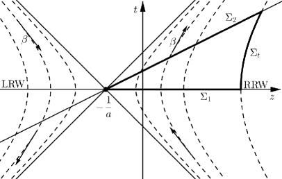
Figure 1: Two-dimensional section of the Minkowski space-time with the Killing field $\beta$ in eq. (15) splitting the plane $tz$ into the Rindler wedges bounded by the light-cone in $z=-1/a$. The integrals of conserved currents on the space-like hypersurfaces $\Sigma_{1}$ and $\Sigma_{2}$ in the RRW are the same because of the Gauss theorem and taking into account that the time-like hyperbolic boundary $\Sigma_{t}$ yields no contribution, being $\beta$ perpendicular to its normal unit vector.

V Entanglement entropy, area law and Unruh effect

The eq. (33) is the entropy current in the RRW, therefore, its integral on a space-like hypersurface having as boundary the 2D surface $z^{\prime}=0,t=0$ (see fig. 1) is

$$S_{R}=\int_{z^{\prime}>0}{\rm d}\Sigma_{\mu}\,s^{\mu}=-{\rm tr}_{R}({\widehat{\rho}}_{R}\log{\widehat{\rho}}_{R})$$ (36)

according to eqs. (20) and (21) and by means of the previous construction of the current. As the density operator is factorized, this entropy is also the entanglement entropy obtained by tracing out the field degrees of freedom in the LRW. At global thermodynamic equilibrium we have $\partial_{\mu}s^{\mu}=0$, and the entropy (36) can be calculated on any space-like hypersurface provided that the boundary flux vanishes. Indeed, this is the case for the RRW, as the time-like boundary is tangent to the entropy current (see fig. 1).

A straightforward calculation of the entanglement entropy on the hypersurface $t=0$ with the canonical entropy current (33) yields:

$$S_{R}=\int_{\mathbb{R}^{2}}{\rm d}x\,{\rm d}y\left(\frac{2\pi^{2}}{45}-\frac{\alpha^{2}}{6}\right)\frac{T_{0}^{3}}{a^{3}}\lim_{z^{\prime}\to 0}\frac{1}{2{z^{\prime}}^{2}}.$$ (37)

Thus, the entropy turns out to be proportional to the area of the 2D boundary surface separating the RRW from the LRW but with a divergent constant, which is owing to the fact that the comoving temperature $T$ diverges for $z^{\prime}=0$. This result is in full agreement with that of Bombelli et al. and Srednicki bombelli ; srednicki .

The same result can be obtained with a more general and more elegant derivation which applies to general space-times. As the entropy current $s$ is divergenceless, $\nabla_{\mu}s^{\mu}=0$, it can be expressed it as the Hodge dual of an exact 3-form. If the domain is topologically contractible (so is the RRW), this form in turn can be expressed as the exterior derivative of a 2-form wald ; oz ; padmanabhan1 ; padmanabhan2 , which eventually amounts to state that the original vector field can be written as the divergence of an anti-symmetric tensor field:

$$s^{\mu}=\nabla_{\nu}\varsigma^{\mu\nu}$$

whence, because of the Stokes’ theorem:

$$S=\int_{\Sigma}{\rm d}\Sigma_{\mu}\;s^{\mu}=\int_{\Sigma}{\rm d}\Sigma_{\mu}\;\nabla_{\nu}\varsigma^{\mu\nu}=\frac{1}{2}\int_{\partial\Sigma}{\rm d}\tilde{S}_{\mu\nu}\,\varsigma^{\mu\nu}=-\frac{1}{4}\int_{\partial\Sigma}{\rm d}S^{\rho\sigma}\;\sqrt{-g}\,\epsilon_{\mu\nu\rho\sigma}\,\varsigma^{\mu\nu}$$ (38)

where ${\rm d}S^{\rho\sigma}$ is the measure of the 2D boundary surface $\partial\Sigma$. Hence, the total entropy is expressed as a surface integral of a potential of a conserved current wald . For our specific problem of equilibrium with acceleration, the general expression of the potential turns out to be:

$$\varsigma^{\mu\nu}=\frac{s}{2\alpha^{2}}\left(\beta^{\mu}\alpha^{\nu}-\beta^{\nu}\alpha^{\mu}\right),$$ (39)

where $s\equiv s^{\mu}u_{\mu}$ is the entropy density. Plugging eq. (39) into eq. (38):

$$S=-\frac{1}{4}\int_{\partial\Sigma}{\rm d}S^{\rho\sigma}\;\sqrt{-g}\frac{s}{2\alpha^{2}}\,\epsilon_{\mu\nu\rho\sigma}\left(\beta^{\mu}\alpha^{\nu}-\beta^{\nu}\alpha^{\mu}\right).$$

The boundary of the hypersurface $t=0$ is the plane $t=0,z^{\prime}=0$ and the plane $t=0,z^{\prime}=+\infty$. In the latter, the integrand vanishes for $s\propto z^{\prime-3}$, $\alpha^{2}$ is constant and $\beta^{0}\alpha^{3}\propto z^{\prime}$. We are thus left with the $xy$ plane and, taking into account that $\rho,\sigma$ indices can only take on values $1,2$ and of the dependence of $\beta$ and $\alpha$ on $(z^{\prime},t)$, we end up with the same eq. (37).

A remarkable consequence of the entropy current method is the determination of the entanglement entropy in the Minkowski vacuum, when the state of the system is pure ${\widehat{\rho}}=|0_{M}\rangle\langle 0_{M}|$. It is well known that crispino :

$${\widehat{\rho}}_{R}={\rm tr}_{L}(|0_{M}\rangle\langle 0_{M}|)=\frac{1}{Z_{R}}\exp\left[-\frac{2\pi}{a}{\widehat{\Pi}}_{R}\right]$$

that is, the Minkowski vacuum for a system with acceleration $a$ corresponds, in the RRW, to a mixed state with density operator (20) with $T_{0}=a/2\pi$, which is in essence the content of the Unruh effect. It was observed in becaunruh that, from a statistical thermodynamics viewpoint, this corresponds to a limiting comoving temperature of $T_{U}=|A|/2\pi$, where $|A|$ is the magnitude of the four-acceleration field. Because of (18), we thus have an upper bound for $|\alpha^{2}|=(2\pi)^{2}$ in the Minkowski vacuum, and so eq. (33) becomes:

$$s^{\mu}=\frac{32\pi^{2}}{45}T^{3}_{U}u^{\mu},$$

while for the eq. (35)

$$s^{\mu}_{\rm IMP}=\frac{2\pi^{2}}{45}T^{3}_{U}u^{\mu}.$$

which mean that we have a non-vanishing entropy current in the Minkowski vacuum, which is owing to having traced out the field degrees of freedom in the LRW. Remarkably, the above expressions differ by a factor 16, which is apparently an unexpected and odd feature. Yet, as it has been mentioned, at global thermodynamic equilibrium the mean value of the stress-energy tensor does depend on the specific quantum operator (in the case at hand, either (30) or (34)) and the entropy current as well. On the other hand, the total integrals like ${\widehat{P}}^{\mu}$ and ${\widehat{J}}^{\mu\nu}$ should not depend on it (see the discussion in ref. becatinti ), and, as a consequence, the entanglement entropy should also be independent because ${\widehat{\rho}}_{R}$ can be written as a trace over the field degrees of freedom of a density operator which is function of the Poincaré generators (see eq. (19)):

$${\widehat{\rho}}_{R}={\rm tr}_{L}({\widehat{\rho}})=\frac{1}{Z}{\rm tr}_{L}\left(\exp\left[-\frac{\widehat{H}}{T_{0}}+\frac{a}{T_{0}}\widehat{K}_{z}\right]\right).$$

Nevertheless, the expressions of ${\widehat{\Pi}}_{R}$ and ${\widehat{\Pi}}_{L}$ (see eqs. (20), (21)) may inherit a dependence on the quantum stress-energy tensor because of the truncation at $z^{\prime}=0$. This issue will be the subject of further investigation.

VI Summary and outlook

In summary, we have presented the condition of existence of an entropy current and a general method to calculate it. An entropy current can be obtained if the spectrum of the local equilibrium operator, which boils down to the Hamiltonian multiplied by $1/T$ in the simplest case of global homogeneous equilibrium, is bounded from below. We have applied our method to the case of a fluid with a comoving acceleration of constant magnitude, a known instance of non-trivial global thermodynamic equilibrium in Minkowski space-time. We have also shown its connection to the entanglement entropy in the vacuum, and its relation with the Unruh effect. Furthermore, we have shown that, at least at global equilibrium, the total entropy can be expressed as a surface integral, in agreement with wald . We expect this method to be applicable to other problems where the total entropy has to be determined, like e.g. relativistic hydrodynamics or thermodynamic equilibrium in general curved space-time.

The entropy current is expectedly dependent on the specific form of the stress-energy tensor operator. Besides, in the case of the free scalar field, the canonical (minimal coupling) and the improved stress-energy tensor (conformal coupling) seem to imply two different results for the total entanglement entropy, even though infinite. This is a subject for future studies.

References

W. Israel, Annals Phys.  100, 310 (1976).

R. Loganayagam, JHEP 0805, 087 (2008)

J. Bhattacharya, S. Bhattacharyya and M. Rangamani, JHEP 1302, 153 (2013).

C. Chattopadhyay, A. Jaiswal, S. Pal and R. Ryblewski, Phys. Rev. C 91, no. 2, 024917 (2015).

R. Banerjee, S. Dey and B. R. Majhi, Phys. Rev. D 92, no. 4, 044019 (2015).

P. Glorioso, M. Crossley and H. Liu, JHEP 1709, 096 (2017).

F. M. Haehl, R. Loganayagam and M. Rangamani, JHEP 1604, 039 (2016).

K. Jensen, R. Marjieh, N. Pinzani-Fokeeva and A. Yarom, JHEP 1901, 061 (2019).

K. Hattori, M. Hongo, X. G. Huang, M. Matsuo and H. Taya, arXiv:1901.06615 [hep-th].

K. Jensen, M. Kaminski, P. Kovtun, R. Meyer, A. Ritz and A. Yarom, Phys. Rev. Lett.  109, 101601 (2012).

S. Bhattacharyya, JHEP 1408, 165 (2014).

S. Bhattacharyya, JHEP 1407, 139 (2014).

F. M. Haehl, R. Loganayagam and M. Rangamani, Phys. Rev. Lett.  121, 051602 (2018).

D. N. Zubarev, A. V. Prozorkevich, S. A. Smolyanskii, Theoret. and Math. Phys. 40, 821 (1979).

Ch. G. Van Weert, Ann. Phys. 140, 133 (1982).

F. Becattini, L. Bucciantini, E. Grossi and L. Tinti, Eur. Phys. J. C 75, no. 5, 191 (2015).

T. Hayata, Y. Hidaka, T. Noumi and M. Hongo, Phys. Rev. D 92, no. 6, 065008 (2015).

M. Buzzegoli and F. Becattini, JHEP 1812, 002 (2018).

F. Becattini, Phys. Rev. Lett.  108, 244502 (2012).

F. Becattini, Phys. Rev. D 97, no. 8, 085013 (2018).

M. Buzzegoli, E. Grossi and F. Becattini, JHEP 1710, 091 (2017) Erratum: [JHEP 1807, 119 (2018)].

J. I. Korsbakken and J. M. Leinaas, Phys. Rev. D 70, 084016 (2004).

L. C. B. Crispino, A. Higuchi and G. E. A. Matsas, Rev. Mod. Phys.  80, 787 (2008).

S. A. Fulling, Phys. Rev. D 7, 2850 (1973).

W. G. Unruh, Phys. Rev. D 14, 870 (1976).

F. Becattini and E. Grossi, Phys. Rev. D 92, 045037 (2015).

F. Becattini and L. Tinti, Phys. Rev. D 84, 025013 (2011).

L. Bombelli, R. K. Koul, J. Lee and R. D. Sorkin, Phys. Rev. D 34, 373 (1986).

M. Srednicki, Phys. Rev. Lett.  71, 666 (1993).

R. M. Wald, Phys. Rev. D 48, no. 8, R3427 (1993).

C. Eling, A. Meyer and Y. Oz, JHEP 1208, 088 (2012).

B. R. Majhi and T. Padmanabhan, Phys. Rev. D 85, 084040 (2012).

B. R. Majhi and T. Padmanabhan, Phys. Rev. D 86, 101501 (2012).

Appendix A Calculation of the entropy potential

The search of a potential for the entropy current uses the same method as for the stress-energy tensor. To form an anti-symmetric tensor we can just use the four-vectors $\beta$ and $\alpha$, hence the only possible combination is:

$$\alpha^{\mu}\beta^{\nu}-\alpha^{\nu}\beta^{\mu}.$$

This is, in turn, just proportional to the thermal vorticity, according to eq. (17), so, we can write the general form of the potential like this:

$$\varsigma^{\mu\nu}=G(\beta^{2},\alpha^{2})\varpi^{\mu\nu}$$ (40)

being $G$ a general scalar function such that:

$$s^{\mu}=\partial_{\nu}\left(G\varpi^{\mu\nu}\right).$$

By introducing the proper entropy density $s$ such that $s^{\mu}u_{\mu}=s$, we have:

$$s=s^{\mu}u_{\mu}=\frac{1}{\sqrt{\beta^{2}}}s^{\mu}\beta_{\mu}=\frac{1}{\sqrt{\beta^{2}}}\beta_{\mu}\varpi^{\mu\nu}\partial_{\nu}G$$

as $\varpi$ is constant. Now, $\varpi^{\mu\nu}\beta_{\mu}=-\sqrt{\beta^{2}}\alpha^{\nu}$ from (17) and so:

$$s=-\alpha^{\nu}\partial_{\nu}G=-\alpha^{\nu}\partial_{\nu}\beta^{2}\frac{\partial G}{\partial\beta^{2}}$$ (41)

because $\alpha^{2}$ is a constant in the pure acceleration case. The Killing equation (11) implies buzzegoli :

$$\partial_{\nu}\beta^{2}=-2\sqrt{\beta^{2}}\alpha_{\nu}$$

so that the (41) becomes:

$$s=2\alpha^{2}\sqrt{\beta^{2}}\frac{\partial G}{\partial\beta^{2}}$$

whose solution is:

$$G=\int{\rm d}\beta^{2}\;\frac{s}{2\alpha^{2}}\frac{1}{\sqrt{\beta^{2}}}.$$

For the massless case, we have $s=C(\alpha)^{2}/\sqrt{\beta^{2}}^{3}$ from (33), hence:

$$G=\frac{C(\alpha^{2})}{2\alpha^{2}}\int{\rm d}\beta^{2}\frac{1}{\beta^{4}}=-\frac{C(\alpha^{2})}{2\alpha^{2}}\frac{1}{\beta^{2}}=-s\frac{2\alpha^{2}}{\sqrt{\beta^{2}}}.$$

Plugging the above result into the (40) and using the (17) we obtain:

$$\varsigma^{\mu\nu}=-\frac{s}{2\alpha^{2}}\sqrt{\beta^{2}}\varpi^{\mu\nu}=-\frac{s}{2\alpha^{2}}\sqrt{\beta^{2}}(\alpha^{\mu}u^{\nu}-\alpha^{\nu}u^{\mu})=\frac{s}{2\alpha^{2}}(\alpha^{\nu}\beta^{\mu}-\alpha^{\mu}\beta^{\nu})$$

which is precisely (39).