Nonlinear management of topological solitons in a spin-orbit-coupled system

Abstract

We consider possibilities to control dynamics of solitons of two types, maintained by the combination of cubic attraction and spin-orbit coupling (SOC) in a two-component system, namely, semi-dipoles (SDs) and mixed modes (MMs), by making the relative strength of the cross-attraction, $\gamma$, a function of time periodically oscillating around the critical value, $\gamma=1$, which is an SD/MM stability boundary in the static system. The structure of SDs is represented by the combination of a fundamental soliton in one component and localized dipole mode in the other, while MMs combine fundamental and dipole terms in each component. Systematic numerical analysis reveals a finite bistability region for the SDs and MMs around $\gamma=1$, which does not exist in the absence of the periodic temporal modulation (“management”), as well as emergence of specific instability troughs and stability tongues for the solitons of both types, which may be explained as manifestations of resonances between the time-periodic modulation and intrinsic modes of the solitons. The system can be implemented in Bose-Einstein condensates, and emulated in nonlinear optical waveguides.

I Introduction

An active direction in the current work with Bose-Einstein condensates (BECs) in atomic gases is using them as a testbed for emulation of various effects originating in condensed-matter physics, which may be reproduced in a clean and easy-to-control form in ultracold bosonic gases simulator ; simulator2 ; simulator3 . In particular, a binary gas, with a pseudo-spinor two-component wave function, may emulate spin-orbit coupling (SOC) in semiconductors, i.e., the interaction between the electron’s spin and its motion across the underlying ionic lattice Dresselhaus ; Rashba , as first demonstrated in Ref. Nature , see also reviews rf:1 -Zhai . While most experimental works on the BEC simulation of SOC dealt with effectively one-dimensional (1D) settings, implementation of SOC in the quasi-2D geometry was reported too 2D-experiment , making it relevant to consider 2D (and 3D) systems coupled by the spin-orbit interaction. In this way, SOC opens a straightforward way to the creation of topological modes characterized by vorticity, because linear operators accounting for the coupling of two components in the corresponding system of Gross-Pitaevskii equations (GPEs), see Eq. (LABEL:GP) below, generate vorticity in one component if the other one is taken in the zero-vorticity form.

The SOC effect, being linear by itself, may be naturally combined with the intrinsic nonlinearity of bosonic gases, represented by cubic terms in the respective GPEs Pit (and/or by nonlocal cubic terms accounting for long-range interactions in BEC built of dipole atoms dip-dip ). The interplay of SOC and nonlinearity makes it possible to predict a great variety of stable modes, including 1D and 2D solitons 1D ; 2D ; Chiquillo ; EPL and various nonlinear topological states in 2D, such as vortices and vortex lattices Fukuoka -Fukuoka10 and skyrmions skyrmion . In fact, the 2D and 3D SOC systems is one of the most prolific sources of nonlinear states with intrinsic topological structures.

A majority of works addressing nonlinear dynamics of SOC systems investigated the case of self-repulsion, which is relevant to the current experiments with ⁸⁷Rb Nature . Nevertheless, the interplay of SOC with intrinsic attraction is possible too. Theoretical considerations predict that the latter setting gives rise to 2D states with intrinsic topological structures and very unusual dynamical properties: until recently, it was commonly assumed that any 2D model with cubic self-attraction may only generate unstable self-trapped states, such as Townes solitons Townes and their vortical counterparts Minsk1 ; Minsk2 . The fundamental (zero-vorticity) Townes solitons are destabilized by the critical collapse (or by the supercritical collapse in 3D), while vortex solitons are subject to a still stronger splitting instability review ; review2 . A new paradigm was revealed by the analysis of the 2D SOC system with cubic self- and cross-attractive interactions Sakaguchi ; Sherman1 ; Sherman2 : the linear SOC terms lift the specific conformal invariance of the cubic GPEs in 2D, which is responsible for the instability, as it makes norms of the entire soliton family degenerate, allowing them to take a single value – exactly the critical one which launches the 2D collapse. As a result of lifting the degeneracy, the norm of the 2D solitons falls below the critical value, thus protecting them against the onset of the collapse Sakaguchi . The specific form of SOC creates two distinct species of topological solitons in this case, namely, semi-vortices (SVs), which combine vorticities $S=0$ and $S=\pm 1$ in the two components, and mixed modes (MMs), which juxtapose zero-vorticity and vortex terms in both components Sakaguchi . Their stability is determined by relative strength $\gamma$ of the cross-attraction between the components and self-attraction (or the XPM/SPM (cross/self-phase modulation) ratio, in terms of optics Maimist ): the SVs and MMs are stable (actually, realizing the system’s ground state) at $\gamma\leq 1$ and $\gamma\geq 1$, respectively. The stability boundary shifts to $\gamma>1$ under the action of the Zeeman splitting Sherman1 . On the other hand, SVs and MMs are stable at all values of $\gamma$ in a model where the self-trapping is provided not by attractive interactions, but by repulsion, with the local strength growing fast enough from the center to periphery Frontiers ; comment ; moreover, even excited states of SVs and MMs, which are completely unstable in the case of the self-attraction Sakaguchi , are partly stable in the latter case.

SOC implemented in 2D BEC as the emulation of the solid-state phenomenology may, in turn, be emulated in optical media, in terms of the spatiotemporal propagation in dual-core planar waveguides, which simulates the pseudo-spinor (two-component) structure of the wave field, while the SOC proper is simulated by temporal optics or spatial we shift of the linear coupling between the parallel waveguiding cores. The former possibility is provided by the known effect of temporal dispersion of the coupling Kip , while the latter scheme may be supported by a skewed structure of the medium separating the cores we . Combining these settings with the natural Kerr self-focusing in the dielectric material opens the way to predict stable 2D optical solitons with an intrinsic topological structure optics ; we , which may be construed as counterparts of the above-mentioned SVs and MMs.

A known method which makes it possible to additionally stabilize soliton modes which are, otherwise, vulnerable to instabilities, is the nonlinearity management, i.e., periodic modulation of the self-focusing strength in time, in the case of BEC Fatkh ; Ueda ; Kevr ; VPG ; breather ; Itin , or along the propagation distance in optics Isaac ; book . In the 2D SOC system, the application of the management technique is an especially interesting possibility, as, by means of the Feshbach resonance controlled by a low-frequency ac magnetic field Feshbach , one can apply time-periodic modulation to the above-mentioned XPM/SPM ratio $\gamma$. As a result, the system will periodically pass from the SV-stability region, $\gamma<1$, to the MM-stability one, $\gamma>1$. Such a possibility poses the problem of the existence and stability of the two species of the 2D solitons in such dynamical states. The situation is somewhat similar to the earlier studied situation with the Feshbach-resonance management periodically alternating the sign of the nonlinearity in the single-component case, which drives periodic transformations between regular and gap-type solitons alternate .

The present work addresses this dynamical problem by means of simulations of GPEs including the SOC terms and the time-modulated coefficient $\gamma$. However, performing such systematic simulations in the 2D model with many control parameters is a challenging numerical problem. On the other hand, it may be efficiently emulated by the similar 1D system, where a counterpart of the SV is a semi-dipole (SD), with a fundamental (spatially even) structure in one component, and a dipole structure (a spatially odd localized state with zero at the central point) in the other (see, e.g., Ref. Chiquillo ). MM states are possible in 1D as well, with the fundamental and dipole terms mixed in both components. A crucially important property of the 1D system, which suggests to use it for the emulation of the 2D prototype which is critically sensitive to the sign of $\gamma-1$, is the fact that, exactly like in 2D, the one-dimensional SDs and MMs are stable, respectively, at $\gamma<1$ and $\gamma>1$, and the nonlinearity-controlling techniques, such as the Feshbach resonance, apply even easier in the 1D settings.

The rest of the paper is organized as follows. The model is introduced in Section II, along with some analytical results which help to illustrate the structure of static SD and MM solitons. Results of the numerical analysis of the management model are collected in Section III. In particular, a region of the SD-MM bistability is found, and qualitative explanations are presented for specific dynamical features (instability troughs and stability tongues) induced by the management. The paper is concluded by Section IV.

II The model and analytical results

In scaled units, the system of GPEs for the 1D binary BEC under the action of the Rashba-type SOC and attractive nonlinearity, takes the form of Sherman1 ; Sherman2

$$i\frac{\partial\phi_{+}}{\partial t} = -\frac{1}{2}\frac{\partial^{2}\phi_{+}}{\partial x^{2}}-(|\phi|_{+}^{2}+\gamma|\phi_{-}|^{2})\phi_{+}+\lambda\frac{\partial\phi_{-}}{\partial x},$$

$$i\frac{\partial\phi_{-}}{\partial t} = -\frac{1}{2}\frac{\partial^{2}\phi_{-}}{\partial x^{2}}-(|\phi|_{-}^{2}+\gamma|\phi_{+}|^{2})\phi_{-}-\lambda\frac{\partial\phi_{+}}{\partial x},$$

where $\phi_{+}$ and $\phi_{-}$ are two components of the pseudo-spinor wave function, $\lambda$ is the SOC strength, self-attraction coefficients are also scaled to be $1$, and $\gamma$ is the above-mentioned relative strength of the nonlinear cross-interaction. By means of scaling transformation,

$$\phi_{\pm}=\lambda\tilde{\phi}_{\pm},~{}x=\lambda^{-1}\tilde{x},~{}t=\lambda^{-2}\tilde{t},$$ (2)

which does not affect $\gamma$, we further fix $\lambda=1$ in Eq. (LABEL:GP) ($\lambda$ is kept as a free parameter in analytical expressions given below by Eqs. (LABEL:SDsmallN)-(12), to make the structure of those expressions clearer). Of course, transformation (2) cannot be applied in the absence of SOC, $\lambda=0$.

Stationary solutions to Eq. (LABEL:GP) of the SD type, with chemical potential $\mu<0$, have the form of

$$\phi_{+}^{(\mathrm{SD})}=e^{-i\mu t}f_{\mathrm{even}}(x),~{}\phi_{-}^{(\mathrm{SD})}=e^{-i\mu t}f_{\mathrm{odd}}(x),$$ (3)

where $f_{\mathrm{even,odd}}(x)$ are even and odd functions, respectively (see, e.g., Eq. (12) below). For the MMs, the appropriate ansatz is

$$\phi_{\pm}^{(\mathrm{MM})}=e^{-i\mu t}\left[f_{\mathrm{even}}(x)\pm f_{\mathrm{odd}}(x)\right].~{}$$ (4)

Stationary modes are characterized by their norm,

$$N\equiv\int_{-\infty}^{+\infty}\left[|\phi_{+}(x)|^{2}+|\phi_{-}(x)|^{2}\right]dx.$$ (5)

As mentioned above, for constant $\gamma=\gamma_{0}$, SDs and MMs are stable, severally, at $\gamma_{0}<1$ and $\gamma_{0}>1$ (in Ref. Sakaguchi , the latter result was originally obtained for SOC of the Rashba type, but it was then established that the same is true for a general Rashba-Dresselhaus combination Sherman1 ). At $\gamma_{0}=1$, both SDs and MMs are marginally stable.

We introduce the nonlinearity management by making $\gamma$ a periodic function of time, the corresponding frequency, $\omega$, being a free parameter of the management:

$$\gamma(t)=\gamma_{0}-\gamma_{1}\sin\left(\omega t\right).$$ (6)

Thus, in our model, with $\lambda=1$ fixed by the scaling, there are four free parameters: $N$, $\gamma_{0}$, $\gamma_{1}$ and $\omega$. We report systematic numerical results for $N=3$, checking that this value adequately represents the generic case. Then, there remain three free parameters to vary: $\gamma_{0}$, $\gamma_{1}$ and $\omega$ in Eq. (6).

While the governing equations are cast here in the scaled form, the rescaling can be undone to estimate characteristic values of control parameters in physical units. In particular, in terms of the BEC realization for light atoms, such as ⁷Li, and the assuming the size of the soliton $\sim 3$ $\mathrm{\mu}$m, the time unit in the scaled equations corresponds to $t_{0}\sim 10$ ms. Then, characteristic scaled values of the management frequencies, $\omega\sim 1$ (see below) correspond, roughly, to $\omega\sim 2\pi\times 20$ Hz.

A more specific situation corresponds to the limit of $N\ll 1$, i.e., broad small-amplitude solitons filled by the striped phase striped , which is represented below by factors $\cos\left(\lambda x\right)$ and $\sin\left(\lambda x\right)$ in Eqs. (LABEL:SDsmallN) and (8). In the absence of the management, they take the following approximate forms, for the SD and MM species, respectively (here, for the clarity’s sake, we keep the SOC strength, $\lambda$, as a free parameter, rather than fixing $\lambda=1$):

$$\phi_{+}^{(\mathrm{SD})}(x) \approx e^{-i\mu t}\frac{\sqrt{3+\gamma}}{4}N~{}\mathrm{sech}\left(\frac{3+\gamma}{8}Nx\right)\cos\left(\lambda x\right),$$

$$\phi_{-}^{(\mathrm{SD})}(x) \approx -e^{-i\mu t}\frac{\sqrt{3+\gamma}}{4}N~{}\mathrm{sech}\left(\frac{3+\gamma}{8}Nx\right)\sin\left(\lambda x\right),$$

$$\phi_{\pm}^{(\mathrm{MM})}(x)\approx e^{-i\mu t}\frac{\sqrt{3+\gamma}}{4\sqrt{2}}N~{}\mathrm{sech}\left(\frac{3+\gamma}{8}Nx\right)\left[\cos\left(\lambda x\right)\pm\sin\left(\lambda x\right)\right],$$ (8)

the chemical potential being $\mu\approx-(1/2)\left[\lambda^{2}+\left(3+\gamma\right)^{2}(N/8)^{2}\right]$ for both species ($\mu\leq-\lambda^{2}/2$ is the semi-infinite spectral gap which may be populated by soliton states).

Another specific case is one corresponding to large $N$, i.e., narrow solitons. In particular, the respective SD state has a large fundamental component,

$$\phi_{+}^{(\mathrm{SD})}\approx\exp\left(-i\frac{N^{2}}{8}t\right)\frac{N}{2}\mathrm{sech}\left(\frac{N}{2}x\right),$$ (9)

while a relatively small dipole one,

$$\phi_{-}^{(\mathrm{SD})}=\exp\left(-i\frac{N^{2}}{8}t\right)u(y),$$ (10)

with $y\equiv Nx/2$ and real function $u(y)$ determined by a linearized equation,

$$\left(\frac{1}{2}-\frac{1}{2}\frac{d^{2}}{dy^{2}}-\gamma~{}\mathrm{sech}^{2}y\right)u=-\lambda\frac{\sinh y}{\cosh^{2}y}.$$ (11)

It is worthy to note that Eq. (11) admits an exact solution precisely in the case of $\gamma=1$, when both SD and MM are stable:

$$u(y)=-\frac{\lambda y}{\cosh y}.$$ (12)

The application of the nonlinearity management to these specific cases should be considered elsewhere.

Simulations of Eq. (LABEL:GP) were run starting with the initial state built as a stable stationary soliton of the SD or MM type (the ground state), produced by means of the imaginary-time-integration method applied to Eq. (LABEL:GP), with $\gamma_{1}=0$ in Eq. (6). Figures 1(a) and (b) display typical profiles of the corresponding static MM and SD states, obtained at $\gamma_{0}=1.1$ and $\gamma_{0}=0.9$, respectively. In the simulations of the full management model, with $\gamma_{1}\neq 0$ in Eq. (6) for various values of $\omega$, stable solitons were identified as those which keep their integrity and initial structure (SD or MM) in the course of long real-time simulations until $t=1000$. Note that, in terms of the above-mentioned estimates for physical parameters of the BEC setting, this corresponds to times $\gtrsim 10$ s, which definitely covers the range of times that may be realized in any experiment.

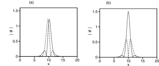
Figure 1: (a) The ground-state soliton of the MM (mixed-mode) type, produced as a numerical solution of Eq. (LABEL:GP) with $\gamma_{1}=0$ in Eq. (6), for $\gamma_{0}=1.1$. (b) A ground-state soliton of the SD (semi-dipole) type, for $\gamma_{0}=0.9$. The solid and dashed lines show the profiles of $|\phi_{+}(x)|$ and $|\phi_{-}(x)|$ respectively.

III Results: stability regions for solitons under the action of the management

Systematic simulations of Eq. (LABEL:GP), with $\gamma$ taken as per Eq. (6), are summarized in Fig. 2, which displays stability regions in the parameter plane of $(\gamma_{0},\omega)$ for the MM- and SD-type solitons, in panels (a) and (b), respectively, with a fixed value of the management amplitude, $\gamma_{1}=0.05$ in Eq. (6). One conclusion is that the application of the management somewhat expands the MM and SD stability areas, from the above-mentioned half-planes in the absence of the management ($\gamma_{1}=0$), i.e., $\gamma_{0}\geq 1$ and $\gamma_{0}\leq 1$, respectively, to values which may be smaller than $\gamma_{0}=1$ for the MMs, and larger than $1$ for the SDs. The expansion gives rise to an MM-SD bistability region, which is presented in detail at the end of this section.

Conspicuous features revealed by Fig. 2 are instability troughs created by the management in the originally stable half-planes. These features may be understood as manifestations of resonant interaction of the ac drive, supplied by the management, and an eigenmode of intrinsic oscillations of stable solitons, existing in the absence of the management. To consider this possibility, the MM’s intrinsic eigenmode and respective eigenfrequency were identified by direct real-time simulations of Eq. (LABEL:GP), with $\gamma_{1}=0$ in Eq. (6), adding a small initial perturbation to the numerically exact MM soliton, as follows:

$$\phi_{+}(x;t=0)=\left(1+\delta\right)\phi_{0+},~{}\phi_{-}(x;t=0)=\left(1-\delta\right)\phi_{0-},$$ (13)

where $\left\{\phi_{0+},\phi_{0-}\right\}$ are the components of the MM state displayed in Fig. 1(a) (i.e., with $\gamma_{0}=1.1$). For the perturbation strength $\delta=0.01$ in Eq. (13), the ensuing evolution of an essential characteristic of the perturbed soliton, which we define as the share of the total norm staying in one component,

$$R(t)=N^{-1}\int_{-\infty}^{+\infty}|\phi_{+}(x)|^{2}dx,$$ (14)

is presented in Fig. 3(a). The evolution of $R(t)$ clearly exhibits eigenfrequency $\omega_{0}\approx 0.34$ of the MM’s intrinsic mode.

The most conspicuous feature in Fig. 2(a) is a relatively wide diagonal instability trough. In particular, at $\gamma_{0}=1.1$ its size is

$$0.585<\omega<0.785.$$ (15)

To consider a possible explanation of this feature in terms of the resonance, in Fig. 3(b) we display a typical example of the instability for $\gamma_{1}=0.05$ at the point taken in the middle of interval (15),

$$\omega/2=0.34\approx\omega_{0}.$$ (16)

The instability is shown by means of the corresponding time dependence for $R(t)$ and the MM’s center-of-mass position,

$$\langle x\rangle=N^{-1}\int_{-\infty}^{+\infty}\left[|\phi_{+}\left(x\right)|^{2}+|\phi_{-}\left(x\right)|^{2}\right]xdx,$$ (17)

together with the modulation format, $\gamma(t)$. The initial condition is taken as Eq. (13) with $\delta=0.001$. The instability manifests itself, in Fig. 3(b), by oscillations of $R(t)$ and $\langle x\rangle$ with a growing amplitude (the spontaneously emerging oscillatory motion of unstable solitons is illustrated by an example displayed below in Fig. 5 (d)). Figure 3(b) shows the initial stage of the perturbation growth. At larger $t$, $R(t)$ exhibits irregular oscillations with an amplitude $\simeq 0.22$ around $R=0.5$. The situation observed in Fig. 3(b) is a typical picture of mechanical instability caused by the parametric resonance with the frequency ratio $1:2$ LL , in agreement with relation (16).

Further, Fig. 3(c) shows the same dynamical characteristics, $R(t)$, $\langle x\rangle$ and $\gamma(t)$ for $\gamma_{0}=1.1$, $\gamma_{1}=0.05$, and $\omega=0.335$, which is a point belonging to the second (much more narrow) instability trough in Fig. 2(a). In this case, the instability is again manifested by the growth of $R(t)$ and $\langle x\rangle$, although the instability is weaker than in Fig. 3(b). Comparing the current value of $\omega$ with $\omega_{0}$ (see Eq. (16)), we conclude that this instability may be interpreted as caused by a direct resonance, with frequency ratio $1:1$. A plausible explanation of additional small “notches” in Fig. 2(a) is the presence of very weak higher-order (subharmonic) resonances. Similarly, the instability-trough pattern observed in Fig. 2(a) can be construed as manifestations of the parametric, direct, and subharmonic resonances with an intrinsic mode of the SD soliton.

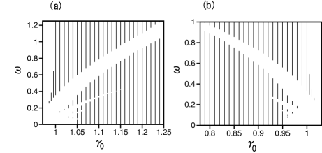
Figure 2: Shaded are stability regions in the parameter plane of $(\gamma_{0},\omega)$ for (a) MM- and (b) SD-type solitons at a fixed management amplitude, $\gamma_{1}=0.05$ in Eq. (6). Solitons are unstable in blank areas.

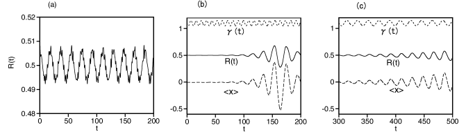
Figure 3: (a) The evolution of the norm ratio $R(t)$ (see Eq. (14)) for the MM, initially perturbed as per Eq. (13), with $\delta=0.01$, at $\gamma_{0}=1.1$ and $\gamma_{1}=0$. (b) The evolution of $R(t)$ (solid line) and $\langle x\rangle$ (dashed line) are shown, along with the underlying modulation format $\gamma(t)$ (Eq. (6), the dotted line), for the MM initiated by input (13) with $\delta=0.001$, at $\gamma_{0}=1.1$, $\gamma_{1}=0.05$, and $\omega=0.68$. (c) The same as in (b), but for $\omega=0.335$.

Another relevant summary of the stability results is presented in Fig. 4 for the solitons of the MM (a) and SD (b) types in parameter plane $(\gamma_{1},\omega)$, fixing the value of the constant term in the nonlinearity coefficient (6), viz., $\gamma_{0}=1.05>1$ in (a), and $\gamma_{0}=0.95<1$ in (b). The solitons are stable at sufficiently large $\omega$, where the high-frequency modulation is effectively averaged out, hence it does not produce a conspicuous effect. It is also natural that stability areas tend to shrink as $\gamma_{1}$ increases. Nevertheless, narrow stability tongues are found too. For example, the SD soliton is stable at $0.265<\omega<0.295$ for $\gamma_{1}=0.12$. Examples of the SD dynamical states, taken at the same fixed value of the management amplitude, $\gamma_{1}=0.12$, are shown in Fig. 5(b) for (a) $\omega=0.31$ (unstable), (b) $\omega=0.28$ (stable), and (c) $\omega=0.25$ (unstable). The stable SD in panel (b) belongs to the narrow “tongue” in Fig. 4(b). It was found that the instability region above the “tongue” is similar to the main instability trough shown in Fig. 2(a).

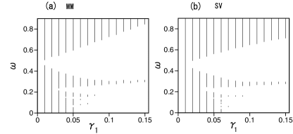
Figure 4: Shaded are stability regions in the parameter plane of the management parameters, $(\gamma_{1},\omega)$ (see Eq. (6)) for MM-type solitons at fixed $\gamma_{0}=1.05$ (a) and SD states (b) at $\gamma_{0}=0.95$.

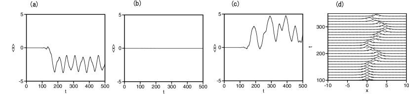
Figure 5: The evolution of the center-of-mass position, $\langle x\rangle$, for the SD solitons, shown along with the underlying time-periodic modulation $\gamma(t)$, with $\gamma_{0}=0.95$ and $\gamma_{1}=0.12$ in Eq. (6), for three values of the modulation frequency: (a) $\omega=0.31$, (b) $\omega=0.28$, and (c) $\omega=0.25$. Panel (d) illustrates the unstable evolution of the soliton corresponding to (c).

While accurate explanation of the nature of the stability tongues requires a more detailed analysis, it is plausible that they also originate from a nonlinear resonance, which, as it is known, gives rise to both unstable and stable solution branches LL .

Lastly, as mentioned above, a noteworthy feature observed in Fig. 2 is bistable coexistence of the SD and MM states in a small but finite region near $\gamma_{0}=1$ (in the absence of the management, $\gamma_{1}=0$, the bistability is only possible strictly at $\gamma_{0}=1$ Sakaguchi ). Figure 6 shows stability boundaries for the SD solitons (solid lines) and MMs (dashed lines) in the parameter space of $(\gamma_{0},\omega)$ (the same plane which is displayed in Fig. 2), at three fixed values of the management amplitude: (a) $\gamma_{1}=0.05$; (b) $\gamma_{1}=0.1$; (c) $\gamma_{1}=0.15$. The SD and MM solitons are stable, severally, in regions bounded by solid lines and dashed ones. Accordingly, the bistability takes place in finite areas between the dashed and solid lines, which are designated by vertical shading in Fig. 6. The bistability region is small, but its size increases with the growth of $\gamma_{1}$.

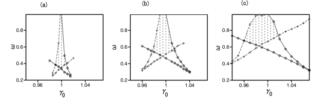
Figure 6: Stability boundaries for the SD and MM dynamical states (solid and dashed lines, respectively) at $\gamma_{1}=0.05$ (a), $\gamma_{1}=0.1$ (b), and $\gamma_{1}=0.15$ (c). The bistability holds between the boundaries, in the vertically-shaded areas (see the text).

IV Conclusion

In this work, we address the possibility to control stability and dynamics of two types of two-component spin-orbit-coupled solitons, SDs (semi-dipoles) and MMs (mixed-modes), which represent distinct species of 1D topological modes, by means of the nonlinearity management, i.e., making the relative strength of the cross-attraction, $\gamma$, a function of time which periodically oscillates around $\gamma=1$. This value is the boundary between stability regions of the static SDs and MMs. By means of systematic simulations, we have found a finite bistability region around $\gamma=1$, which expands with the increase of the management amplitude. In the usual SDs’ and MMs’ stability domains ($\gamma<1$ and $\gamma>1$, respectively), the analysis reveals new features generated by the management, in the form of long instability troughs and, on the other hand, stability tongues penetrating into instability domains. These features may be explained as manifestations of resonances between the time-periodic management and excitation modes of stable 2D solitons, that exist in the absence of the management.

As said above, the 1D soliton species of the SD and MM types emulate their 2D spin-orbit-coupled counterparts, in the form of SVs (semi-vortices) and two-dimensional MMs, respectively. It may be quite interesting, although somewhat challenging, in terms of collecting systematical numerical data, to identify stability charts for the 2D topological modes of both types under the action of the nonlinearity management. Another relevant extension may be realization of the nonlinearity management for the two-component system combining SOC and long-range dipole-dipole interactions Guangzhou . It may be realized by periodically varying the direction of the external magnetic field which determines the orientation of the atomic magnetic moments.

References

- (1) P. Hauke, F. M. Cucchietti, and L. Tagliacozzo, I. Deutsch, and M. Lewenstein, Can one trust quantum simulators? Rep. Prog. Phys. 2012,75, 082401
- (2) T. H. Johnson, S. R. Clark, and D. Jaksch, What is a quantum simulator? EPJ Quantum Technology 2014, 1, 10.
- (3) E. Zohar, J. I. Cirac, and B. Reznik, Quantum simulations of lattice gauge theories using ultracold atoms in optical lattices. Rep. Prog. Phys. 2016, 79, 014401.
- (4) G. Dresselhaus, Spin-orbit coupling effects in zinc blende structures. Phys. Rev. 1955, 100, 580–586.
- (5) Y. A. Bychkov and E. I. Rashba, Oscillatory effects and the magnetic-susceptibility of carriers in inverse-layers. J. Phys. C 1984, 17, 6039–6045.
- (6) Y. J. Lin, K. Jimenez-Garcia, and I. B. Spielman, Spin-orbit-coupled Bose-Einstein condensates. Nature 2011, 471, 83–86.
- (7) J. Dalibard, F. Gerbier, G. Juzeliūnas, and P. Öhberg, Artificial gauge potentials for neutral atoms. Rev. Mod. Phys. 2011, 83, 1523–1543.
- (8) V. Galitski and I. B. Spielman, Spin-orbit coupling in quantum gases. Nature 2013, 494, 49–54.
- (9) X. Zhou, Y. Li, Z. Cai, and C. Wu, Unconventional states of bosons with the synthetic spin-orbit coupling. J. Phys. B: At. Mol. Opt. Phys. 2013, 46, 134001.
- (10) N. Goldman, G. Juzeliūnas, P. Öhberg, and I. B. Spielman, Light-induced gauge fields for ultracold atoms. Rep. Progr. Phys. 2014, 77, 126401.
- (11) H. Zhai, Degenerate quantum gases with spin–orbit coupling: a review. Rep. Prog. Phys. 2015, 78, 026001.
- (12) Z. Wu, L. Zhang, W. Sun, X.-T. Xu, B.-Z. Wang, S.-C. Ji, Y. Deng, S. Chen, X.-J. Liu, and J.-W. Pan, Realization of two-dimensional spin-orbit coupling for Bose-Einstein condensates. Science 2016, 354, 83–88.
- (13) L. P. Pitaevskii and S. Stringari, Bose-Einstein Condensation; Oxford University Press, Oxford, 2003.
- (14) T. Lahaye, C. Menotti, L. Santos, M. Lewenstein, and T. Pfau, The physics of dipolar bosonic quantum gases. Rep. Prog. Phys. 2009, 72, 26401.
- (15) Y. V. Kartashov and V. V. Konotop, Solitons in Bose-Einstein condensates with helicoidal spin-orbit coupling. Phys. Rev. Lett. 2017, 118, 190401.
- (16) V. E. Lobanov, Y. V. Kartashov, and V. V. Konotop, Fundamental, multipole, and half-vortex gap solitons in spin-orbit coupled Bose-Einstein condensates. Phys. Rev. Lett. 2014, 112, 180403.
- (17) E. Chiquillo, 105001 (2017), Harmonically trapped attractive and repulsive spin-orbit and Rabi coupled Bose-Einstein condensates. J. Phys. A: Math. Theor. 2017, 50, 105001.
- (18) B. A. Malomed, Creating solitons by means of spin-orbit coupling. EPL 2018, 122, 36001.
- (19) S. Sinha, R. Nath, and L. Santos, Trapped two-dimensional condensates with synthetic spin-orbit coupling. Phys. Rev. Lett. 2011, 107, 270401.
- (20) C. J. Wu, I. Mondragon-Shem, and X.-F. Zhou, Unconventional Bose-Einstein Condensations from Spin-Orbit Coupling. Chin. Phys. Lett. 2011, 28, 097102.
- (21) Y. Deng, J. Cheng, H. Jing, C. P. Sun, and S. Yi, Spin-orbit-coupled dipolar Bose-Einstein condensates. Phys. Rev. Lett. 2012, 108, 125301.
- (22) T. Kawakami, T. Mizushima, and K. Machida, Textures of spinor Bose-Einstein condensates with spin-orbit coupling. Phys. Rev. A 2011, 84, 011607.
- (23) B. Ramachandhran, B. Opanchuk, X.-J. Liu, H. Pu, P. D. Drummond, and H. Hu, Half-quantum vortex state in a spin-orbit-coupled Bose-Einstein condensate. Phys. Rev. A 2012, 85, 023606.
- (24) G. J. Conduit, Line of Dirac monopoles embedded in a Bose-Einstein condensate. Phys. Rev. A 2012, 86, 021605(R).
- (25) E. Ruokokoski, J. A. M. Huhtamäki, and M. Möttönen, Stationary states of trapped spin-orbit-coupled Bose-Einstein condensates. Phys. Rev. A 2012, 86, 051607.
- (26) H. Sakaguchi and B. Li, Vortex lattice solutions to the Gross-Pitaevskii equation with spin-orbit coupling in optical lattices. Phys. Rev. A 2013, 87, 015602.
- (27) A. Fetter, Vortex dynamics in spin-orbit-coupled Bose-Einstein condensates. Phys. Rev. A 2014, 89, 023629.
- (28) H. Sakaguchi and K. Umeda, Solitons and vortex lattices in the Gross-Pitaevskii equation with spin-orbit coupling under rotation. J. Phys. Soc. Jpn. 2016, 85, 064402.
- (29) T. Kawakami, T. Mizushima, M. Nitta, and K. Machida, Stable skyrmions in gauged Bose-Einstein condensates. Phys. Rev. Lett. 2012, 109, 015301.
- (30) R. Y. Chiao, E. Garmire, and C. H. Townes, Self-trapping of optical beams. Phys. Rev. Lett. 1964, 13, 479–482.
- (31) V. I. Kruglov and R. A. Vlasov, Spiral self-trapping propagation of optical beams. Phys. Lett. A 1985, 111, 401–404.
- (32) V. I. Kruglov, Yu. A. Logvin, and V. M. Volkov, The theory of spiral laser beams in nonlinear media. J. Mod. Opt. 1992, 39, 2277–2291.
- (33) L. Bergé, Wave collapse in physics: principles and applications to light and plasma waves, Phys. Rep. 303, 259-370 (1998).
- (34) G. Fibich, Nonlinear Schrödinger Equation: Singular Solutions and Optical Collapse; Springer: Heidelberg, 2015.
- (35) B. A. Malomed, D. Mihalache, F. Wise, and L. Torner, Spatiotemporal optical solitons. J. Optics B: Quant. Semicl. Opt. 2005, 7, R53–R72; Viewpoint: On multidimensional solitons and their legacy in contemporary Atomic, Molecular and Optical physics. J. Phys. B: At. Mol. Opt. Phys. 2016, 49, 170502.
- (36) Y. Kartashov, G. Astrakharchik, B. Malomed, and L. Torner, Frontiers in multidimensional self-trapping of nonlinear fields and matter. Nature Reviews Physics 2019, 1, 185-197.
- (37) H. Sakaguchi, B. Li, and B. A. Malomed, Creation of two-dimensional composite solitons in spin-orbit-coupled self attractive Bose-Einstein condensates in free space. Phys. Rev. E 2014, 89, 0329020.
- (38) H. Sakaguchi, E. Ya. Sherman, and B. A. Malomed, Vortex solitons in two-dimensional spin-orbit coupled Bose-Einstein condensates: Effects of the Rashba-Dresselhaus coupling and the Zeeman splitting. Phys. Rev. E 2016, 94, 032202.
- (39) H. Sakaguchi, B. Li, E. Ya. Sherman, and B. A. Malomed, Composite solitons in two-dimensional spin-orbit coupled self-attractive Bose-Einstein condensates in free space. Romanian Reports in Physics 2018, 70, 502.
- (40) A. I. Maimistov, Solitons in nonlinear optics. Quantum Electron. 2010, 40, 756.
- (41) R. Zhong, Z. Chen, C. Huang, Z. Luo, H. Tan, B. A. Malomed, and Y. Li, Self-trapping under the two-dimensional spin-orbit-coupling and spatially growing repulsive nonlinearity. Front. Phys. 2018, 13, 130311.
- (42) H. Sakaguchi, New models for multi-dimensional stable vortex solitons. Frontiers of Physics 2019, 14, 1230.
- (43) Y. V. Kartashov, B. A. Malomed, V. V. Konotop, V. E. Lobanov, and L. Torner, Stabilization of solitons in bulk Kerr media by dispersive coupling. Opt. Lett. 2015, 40, 1045–1048.
- (44) H. Sakaguchi and B. A. Malomed, One- and two-dimensional solitons in -symmetric systems emulating spin–orbit coupling. New J. Phys. 2016, 18, 105005.
- (45) K. S. Chiang, Intermodal dispersion in 2-core optical fibers. Opt. Lett. 1995, 20, 997–999.
- (46) F. Kh. Abdullaev, J. G. Caputo, R. A. Kraenkel, and B. A. Malomed, Controlling collapse in Bose-Einstein condensation by temporal modulation of the scattering length, Phys. Rev. A 67, 013605 (2003).
- (47) H. Saito and M. Ueda, Dynamically stabilized bright solitons in a two-dimensional Bose-Einstein condensate. Phys. Rev. Lett. 2003, 90, 040403.
- (48) P. G. Kevrekidis, G. Theocharis, D. J. Frantzeskakis, and B. A. Malomed, Feshbach resonance management for Bose-Einstein condensates. Phys. Rev. Lett. 2003, 90, 230401.
- (49) G. D. Montesinos, V. M. Perez-Garcia, and H. Michinel, Stabilized two-dimensional vector solitons. Phys. Rev. Lett. 2004, 92, 133901.
- (50) H. Sakaguchi and B. A. Malomed, Resonant nonlinearity management for nonlinear Schrödinger solitons. Phys. Rev. E 2004, 70, 066613.
- (51) A. Itin, T. Morishita, and S. Watanabe, Reexamination of dynamical stabilization of matter-wave solitons. Phys. Rev. A 2006, 74, 033613.
- (52) I. Towers and B. A. Malomed, Stable (2+1)-dimensional solitons in a layered medium with sign-alternating Kerr nonlinearity. J. Opt. Soc. Am. B 2002, 19, 537–543.
- (53) B. A. Malomed, Soliton Management in Periodic Systems; Springer, New York, 2006.
- (54) S. B. Papp, J. M. Pino, and C. E. Wieman, Tunable miscibility in a dual-species Bose-Einstein condensate. Phys. Rev. Lett. 2008, 101, 040402.
- (55) A. Gubeskys, B. A. Malomed, and I. M. Merhasin. Alternate solitons: Nonlinearly-managed one- and two-dimensional solitons in optical lattices. Stud. Appl. Math. 2005, 115, 255–277.
- (56) V. Achilleos, D. J. Frantzeskakis, P. G. Kevrekidis, and D. E. Pelinovsky, Matter-wave bright solitons in spin-orbit coupled Bose-Einstein condensates. Phys. Rev. Lett. 2013, 110, 264101.
- (57) L. D. Landau and E. M. Lifshitz, Mechanics; Nauka Publishers: Moscow, 1988.
- (58) X. Jiang, Z. Fan, Z. Chen, W. Pang, Y. Li, and B. A. Malomed, Two-dimensional solitons in dipolar Bose-Einstein condensates with spin-orbit coupling. Phys. Rev. A 2016, 93, 023633.