Conditional past-future correlation in dephasing environments

Break of conditional past-future independence induced by non-Markovian dephasing baths

Conditional past-future correlation induced by non-Markovian dephasing reservoirs

Abstract

Memory effects can be studied through a conditional past-future correlation, which measures departure with respect to a conditional past-future independence valid in a memoryless Markovian regime. In a quantum regime this property leads to an operational definition of quantum non-Markovianity based on three consecutive system measurement processes and postselection [Budini, Phys. Rev. Lett. 121, 240401 (2018)]. Here, we study the conditional past-future correlation for a qubit system coupled to different dephasing environments. Exact solutions are obtained for a quantum spin bath as well as for classically fluctuating random Hamiltonian models. The developing of memory effects and departures from Born-Markov or white-noise approximations are related to a measurement back action that changes the system dynamics between consecutive measurements. It is shown that this effect may develop even when the former system evolution is given by a time-independent Lindblad equation. This unusual non-Markovian case arises when the characteristic parameters of the dynamics become Lorentzian random distributed variables.

I Introduction

In a classical regime, Markovianity (memoryless property) leads to descriptions based on local-in-time evolutions such as Fokker-Planck equations and master equations vanKampen . In a quantum regime, instead of probabilities, a density matrix operator describes the open system dynamics breuerbook ; vega . As is well known, when a local-in-time description applies the evolution of the density matrix must to assume a Lindblad structure alicki . Therefore, in the last years these equations were naturally related to quantum Markovianity. In fact, different quantum memory measures (quantum non-Markovianity measures) rely on diverse departures that a system may develops with respect to their properties BreuerReview ; plenioReview . Many alternative proposals were studied BreuerFirst ; cirac ; rivas ; DarioSabrina ; BaeDario ; dario11 ; Acin ; cresser ; canonicalCresser ; geometrical ; fisher ; mutual ; brasil ; fidelity ; eternal ; maximal , most of them based on the behavior of different quantum information measures under a Lindblad evolution.

Usually in the definition of the previous memory indicators the only available information is given by the density matrix evolution or propagator. Memory effects developing in open quantum systems can also be defined on alternative grounds. For example, the well-established notion of classical Markovianity vanKampen can be extended to a quantum regime by subjecting the system to extra control operations (measurements) modi ; PRL . The operational definition of quantum Markovianity introduced in Ref. modi is based on a “process tensor” framework, which relies on the usual definition of classical Markovianity in terms of conditional probability distributions. Thus, quantum Markovianity is defined by a conditional independence of the system dynamics on past control operations.

The formalism of Ref. PRL relies on an equivalent but different formulation of classical Markovianity, that is, the statistical independence of past and future events when conditioned to a given state at the present time CoverTomas . Equivalently, memory effects break conditional past-future (CPF) independence. Hence, an ensemble of three time-ordered (random) system events provides a minimal basis for establishing classical and quantum Markovianity. A related conditional past-future correlation becomes an univocal indicator of departures from a memoryless regime. In a quantum regime, the three events correspond to the outcomes of three (system) measurement processes. Postselection take into account the conditional character of the definition. The CPF correlation vanishes whenever a Born-Markov or white noise approximation applies to quantum or classical environments respectively PRL . Its calculation involves both predictive and retrodicted quantum probabilities vaidman ; murch ; molmer . Hence, techniques and concepts coming from retrodicted quantum measurements vaidman ; murch ; molmer ; haroche ; huard ; naghi ; decay ; retro ; wiseman ; dressel ; barnett play a fundamental role in this alternative approach.

In this paper we study the CPF correlation for a qubit system interacting with different non-Markovian dephasing environments such as a quantum spin bath and stochastic Hamiltonian models. An explicit derivation complement the exact results presented in Ref. PRL . In addition, the developing of memory effects and departure from Born-Markov and white noise approximations are studied in detail for both kinds of models. These features are related to a measurement back action that changes the system dynamics between consecutive measurements processes. Contrarily to all previous non-Markovian measures BreuerReview ; plenioReview , we explicitly show that even when a time-independent Lindblad equation defines the former system evolution (between the first and second measurements), its posterior dynamics (between the second and third measurements) can be modified. This unusual non-Markovian dynamics arises in both kinds of models when the underlying parameters become random (time-independent) variables characterized by a Lorentzian probability density.

The paper is outlined as follows. In Sec. II we briefly resume the formalism established in Ref. PRL . In Sec. III the spin bath model is studied. Sec. IV is devoted to stochastic Hamiltonian dynamics. In Sec. V, both kinds of models are characterized when the underlying parameters become Lorentzian random variables. The conclusions are provided in Sec. VI.

II Conditional past-future correlation

Given an ensemble of three time ordered random events $x\rightarrow y\rightarrow z$ occurring at times $t_{x}<t_{y}<t_{z},$ Bayes rule allow us to write the probability $P(z,x|y)$ of past $(x)$ and future events $(z),$ conditioned to a given present state $(y),$ as

$$P(z,x|y)=P(z|y,x)P(x|y),$$ (1)

where in general $P(b|a)$ denotes the conditional probability of $b$ given $a.$ A conditional past-future correlation,

$$C_{pf}=\langle O_{z}O_{x}\rangle_{y}-\langle O_{z}\rangle_{y}\langle O_{x}\rangle_{y},$$ (2)

defined as

$$C_{pf}=\sum_{zx}[P(z,x|y)-P(z|y)P(x|y)]O_{z}O_{x},$$ (3)

is a measure of memory non-Markovian effects PRL . In fact, for Markovian processes $P(z|y,x)=P(z|y),$ implying $P(z,x|y)=P(z|y)P(x|y).$ Thus, $C_{pf}=0.$ In Eq. (3) the sum indexes $z$ and $x$ run over all possible outcomes occurring at times $t_{z}$ and $t_{x}$ respectively, while $y$ is a fixed particular possible value at time $t_{y}.$ The parameters $\{O_{z}\}$ and $\{O_{x}\}$ correspond to a property associated to each system state.

In a quantum regime, the sequence $x\rightarrow y\rightarrow z$ is given by the outcomes of three consecutive measurements performed over the system of interest. The corresponding measurement operators milburn are $x\rightarrow\Omega_{x},$ $y\rightarrow\Omega_{y},$ $z\rightarrow\Omega_{z},$ and fulfill $\sum_{x}\Omega_{x}^{{\dagger}}\Omega_{x}=\sum_{y}\Omega_{y}^{{\dagger}}\Omega_{y}=\sum_{z}\Omega_{z}^{{\dagger}}\Omega_{z}=\mathrm{I},$ where $\mathrm{I}$ is the identity matrix in the system Hilbert space and the sum indexes run over all possible outcomes at each stage. Furthermore, in Eq. (3) $\{O_{z}\}$ and $\{O_{x}\}$ are set by the measured observables. Given the conditional character of the past-future correlation, in an experimental setup it follows from a postselected sub-ensemble of realizations where the intermediate $y$-outcome is a fixed arbitrary one. On the other hand, the calculation of $P(z|y,x)$ relies on standard predictive quantum measurement theory. In contrast, $P(x|y)$ is a retrodicted probability that can be read from a “past quantum state” formalism molmer ; retro .

III Dephasing spin bath

Similarly to Ref. PRL , here we consider a qubit system interacting with a quantum spin bath Zurek ; ZurekRMP ; Paz . Their mutual interaction is set by the Hamiltonian

$$H_{T}=\sigma_{\hat{z}}\otimes\sum_{k=1}^{N}g_{k}\sigma_{\hat{z}}^{(k)}.$$ (4)

In here, $\sigma_{\hat{z}}$ is the system Pauli matrix in the $\hat{z}-$direction. Its eigenvectors are denoted as $|\pm\rangle.$ On the other hand, $\sigma_{\hat{z}}^{(k)}$ is the $\hat{z}-$Pauli matrix corresponding to the $k$-spin, whose eigenvectors are denoted as $|\uparrow\rangle_{k}$ and $|\downarrow\rangle_{k}.$ $\{g_{k}\}$ measure the coupling between each spin of the environment and the qubit.

The interaction model (4) always admits an exact solution Zurek ; ZurekRMP ; Paz . For a separable pure initial bipartite state, $\rho_{0}^{se}=|\Psi_{0}\rangle\langle\Psi_{0}|,$ with

$$|\Psi_{0}\rangle=(a|+\rangle+b|-\rangle)\otimes\sum_{k=1}^{N}(\alpha_{k}|\uparrow\rangle_{k}+\beta_{k}|\downarrow\rangle_{k}),$$ (5)

where the initial bath state is sets by the individual spin coefficients $\{\alpha_{k}\}$ and $\{\beta_{k}\},$ at time $t$ the bipartite state is $\rho_{t}^{se}=|\Psi_{t}\rangle\langle\Psi_{t}|,$ where

$$|\Psi_{t}\rangle=a|+\rangle\otimes|\mathcal{B}(t)\rangle+b|-\rangle\otimes|\mathcal{B}(-t)\rangle.$$ (6)

Thus, the system and the environment become entangled. The normalized bath state $[\langle\mathcal{B}(t)|\mathcal{B}(t)\rangle=1]$ is ZurekRMP ; Paz

$$|\mathcal{B}(t)\rangle=\prod_{k=1}^{N}(\alpha_{k}e^{+i2g_{k}t}|\uparrow\rangle+\beta_{k}e^{-i2g_{k}t}|\downarrow\rangle).$$ (7)

The three measurement processes that define the CPF correlation [Eq. (3)] are chosen as projective ones, all of them being performed in $\hat{x}$-direction of the qubit Bloch sphere. Thus, the outcomes of each measurement, in successive order, are $x=\pm 1,$ $y=\pm 1,$ and $z=\pm 1,$ which in turn define the system operators values $O_{z}=z$ and $O_{x}=x.$ The corresponding measurement operators are the same, $\{\Omega_{x}\}=\{\Omega_{y}\}=\{\Omega_{z}\}=\{\Pi_{\hat{x}=\pm 1}\},$ where $\Pi_{\hat{x}=\pm 1}=|\hat{x}_{\pm}\rangle\langle\hat{x}_{\pm}|,$ with $|\hat{x}_{\pm}\rangle=(|+\rangle\pm|-\rangle)/\sqrt{2}.$ A hat symbol distinguishes directions in Bloch sphere from measurement outcomes.

III.1 Conditional probabilities

In the following calculations the initial system state is $|+\rangle$ [Eq. (5) with $a=1$ and $b=0].$ Thus,

$$|\Psi_{0}\rangle=|+\rangle\otimes\sum_{k=1}^{N}(\alpha_{k}|\uparrow\rangle_{k}+\beta_{k}|\downarrow\rangle_{k}),$$ (8)

is the initial bipartite system-environment state. The goal is to calculate $P(x|y)$ and $P(z|y,x)$ [Eq. (1)].

At all steps the bipartite state remains a pure one. After the first $x$-measurement, from standard quantum measurement theory milburn , it becomes $|\Psi_{0}\rangle\rightarrow|\Psi_{0}^{x}\rangle=\Pi_{\hat{x}=x}|\Psi_{0}\rangle/\sqrt{\langle\Psi_{0}|\Pi_{\hat{x}=x}|\Psi_{0}\rangle},$ delivering

$$|\Psi_{0}^{x}\rangle=\frac{|+\rangle+x|-\rangle}{\sqrt{2}}\otimes\sum_{k=1}^{N}(\alpha_{k}|\uparrow\rangle_{k}+\beta_{k}|\downarrow\rangle_{k}),$$ (9)

where consistently $x=\pm 1$ is the outcome of the first measurement. The probability of both options is $P(x)=\langle\Psi_{0}|\Pi_{\hat{x}=x}|\Psi_{0}\rangle=1/2.$

After evolving up to a time $t\equiv t_{y}-t_{x},$ from Eq. (6) the bipartite state becomes

$$|\Psi_{t}^{x}\rangle=\frac{1}{\sqrt{2}}(|+\rangle\otimes|\mathcal{B}(t)\rangle+x|-\rangle\otimes|\mathcal{B}(-t)\rangle).$$ (10)

Posteriorly, the second measurement, with outcomes $y=\pm 1,$ is performed in $\hat{x}-$direction. The probability of each option, given that the previous outcome was $x,$ is $P(y|x)=\langle\Psi_{t}^{x}|\Pi_{\hat{x}=y}|\Psi_{t}^{x}\rangle,$ which delivers $P(y|x)=(1+yx\mathrm{Re}[\langle\mathcal{B}(-t)|\mathcal{B}(t)\rangle])/2.$ Introducing the joint probability of both outcomes $P(y,x)=P(y|x)P(x),$

$$P(y,x)=\frac{1}{4}(1+yx\mathrm{Re}[\langle\mathcal{B}(-t)|\mathcal{B}(t)\rangle]),$$ (11)

it follows $P(y)=\sum_{x=\pm 1}P(y,x)=1/2.$ The retrodicted probability $P(x|y)=P(y,x)/P(y)$ then reads

$$P(x|y)=\frac{1}{2}(1+yx\mathrm{Re}[\langle\mathcal{B}(-t)|\mathcal{B}(t)\rangle]).$$ (12)

Due to the chosen system initial condition, it follows the symmetry $P(x|y)=P(y|x).$

After the second $y$-measurement the bipartite state change as $|\Psi_{t}^{x}\rangle\rightarrow|\Psi_{t}^{yx}\rangle=\Pi_{\hat{x}=y}|\Psi_{t}^{x}\rangle/\sqrt{\langle\Psi_{t}^{x}|\Pi_{\hat{x}=y}|\Psi_{t}^{x}\rangle},$ which from Eq. (10) reads

$$|\Psi_{t}^{yx}\rangle=\frac{|+\rangle+y|-\rangle}{\sqrt{2}}\otimes|\mathcal{B}_{yx}(t)\rangle.$$ (13)

The bath state is

$$|\mathcal{B}_{yx}(t)\rangle\equiv\frac{|\mathcal{B}(t)\rangle+yx|\mathcal{B}(-t)\rangle}{\sqrt{\mathcal{N}_{t}^{yx}}},$$ (14)

with normalization constant $\mathcal{N}_{t}^{yx}=\langle\mathcal{B}(t)|\mathcal{B}(t)\rangle+\langle\mathcal{B}(-t)|\mathcal{B}(-t)\rangle+yx(\langle\mathcal{B}(t)|\mathcal{B}(-t)\rangle+\langle\mathcal{B}(-t)|\mathcal{B}(t)\rangle).$ It can be rewritten as $\mathcal{N}_{t}^{yx}=4P(x|y)$ [Eq. (12)].

In the next step, the bipartite arrangement evolves during a time interval $\tau\equiv t_{z}-t_{y}$ with the unitary dynamics dictated by the Hamiltonian (4), $|\Psi_{t}^{yx}\rangle\rightarrow|\Psi_{t+\tau}^{yx}\rangle.$ From Eq. (6) it follows

$$|\Psi_{t+\tau}^{yx}\rangle=\frac{1}{\sqrt{2}}(|+\rangle\otimes|\mathcal{B}_{yx}(t+\tau)\rangle+y|-\rangle\otimes|\mathcal{B}_{yx}(t-\tau)\rangle).$$ (15)

The probability of the last $z$-measurement $P(z|y,x)=\langle\Psi_{t+\tau}^{yx}|\Pi_{\hat{x}=z}|\Psi_{t+\tau}^{yx}\rangle,$ reads

$$P(z|y,x)=\frac{1}{2}(1+zy\mathrm{Re}[\langle\mathcal{B}_{yx}(t-\tau)|\mathcal{B}_{yx}(t+\tau)\rangle]).$$ (16)

Eqs. (12) and (16) are the central results of this subsection.

III.2 Dynamics between consecutive measurements

The previous analysis allows us to characterize the system dynamics between consecutive measurement events. After the first $x$-measurement and before the second $y$-measurement [time interval $(0,t)],$ the system state follows as $\rho_{t}^{x}=\mathrm{Tr}_{e}[|\Psi_{t}^{x}\rangle\langle\Psi_{t}^{x}|],$ where $|\Psi_{t}^{x}\rangle$ is given by Eq. (10), and $\mathrm{Tr}_{e}[\cdot]$ is the trace operation over the environment degrees of freedom. We get,

$$\rho_{t}^{x}=\frac{1}{2}\left(\begin{array}[]{cc}1&xc_{t}\\ xc_{t}^{\ast}&1\end{array}\right),$$ (17)

where the coherence behavior, from Eq. (7), is given by

$$c_{t}\equiv\langle\mathcal{B}(-t)|\mathcal{B}(t)\rangle=\prod_{k=1}^{N}(|\alpha_{k}|^{2}e^{+i2g_{k}t}+|\beta_{k}|^{2}e^{-i2g_{k}t}).$$ (18)

Consistently with the underlying interaction [Eq. (4)], only the system coherences are affected.

After the second $y$-measurement and before the third $z$-measurement [time interval $(t,t+\tau)],$ the system state follows as $\rho_{t,\tau}^{yx}=\mathrm{Tr}_{e}[|\Psi_{t+\tau}^{yx}\rangle\langle\Psi_{t+\tau}^{yx}|],$ where $|\Psi_{t+\tau}^{yx}\rangle$ is given by Eq. (15). We get,

$$\rho_{t,\tau}^{yx}=\frac{1}{2}\left(\begin{array}[]{cc}1&yc_{t,\tau}^{yx}\\ yc_{t,\tau}^{yx\ast}&1\end{array}\right),$$ (19)

where the new coherence behavior $c_{t,\tau}^{yx},$ from Eq. (14), is given by

$$c_{t,\tau}^{yx}\equiv\langle\mathcal{B}_{yx}(t-\tau)|\mathcal{B}_{yx}(t+\tau)\rangle\!=\!\frac{c_{\tau}+yx(c_{t+\tau}+c_{t-\tau}^{\ast})/2}{1+yx(c_{t}+c_{t}^{\ast})/2}.$$ (20)

Here, $c_{t}$ gives the previous coherence behavior, Eq. (18). In contrast, $c_{t,\tau}^{yx}$ explicitly depends on both previous measurement results.

From Eqs. (10) and (15), it is evident that for this model a Born-Markov approximation breuerbook ; vega does not applies at any stage (separable system-bath state). This non-Markovian property can also be read from a measurement back action that leads to a change of system dynamics between consecutive measurements, $c_{t,\tau}^{yx}\neq c_{t}.$

The former bipartite dynamics in $(0,t)$ begins in a separable state [Eq. (9)]. Due to the projective nature of the second $y$-measurement, this property is also valid for the interval $(t,t+\tau)$ [Eq. (13)]. Nevertheless, in contrast here the bath state $|\mathcal{B}_{yx}(t)\rangle$ is an entangled one that involves all spin bath variables [Eq. (14)]. It is a superposition of the bath states $|\mathcal{B}(t)\rangle$ and $|\mathcal{B}(-t)\rangle$ whose phase in turn depends on the product of outcomes $yx.$ This measurement back action on the bath degrees of freedom leads to a different posterior system dynamics. Thus, this change can in fact be read as a fingerprint of non-Markovian effects and departure from Born-Markov approximation.

III.3 CPF correlation

The CPF correlation (3) can be calculated after getting the CPF probability $P(z,x|y)=P(z|y,x)P(x|y).$ From Eqs. (12) and (16), jointly with Eqs. (18) and (20), it follows

$$P(z,x|y) = \frac{1}{4}\Big{\{}1+xyf(t)+zyf(\tau)$$ (21)

$$+zx\frac{[f(t+\tau)+f(t-\tau)]}{2}\Big{\}},$$

where for simplifying the expression we defined $f(t)\equiv\mathrm{Re}[c_{t}].$ In addition,

$$P(z|y) = \sum_{x=\pm 1}P(z,x|y)=\frac{1}{2}[1+zyf(\tau)],$$ (22a)

$$P(x|y) = \sum_{z=\pm 1}P(z,x|y)=\frac{1}{2}[1+xyf(t)].$$ (22b)

The conditional averages then reads $$\langle O_{z}\rangle_{y}=yf(\tau), \langle O_{x}\rangle_{y}=yf(t), \langle O_{z}O_{x}\rangle_{y}=[f(t+\tau)+f(t-\tau)]/2, O_{z}=z, O_{x}=x. [C_{pf}\rightarrow C_{pf}(t,\tau)]$$ while from Eq. (21) we get where it has been used that The exact expression for the CPF correlation (3) then is

$$C_{pf}(t,\tau)=\frac{f(t+\tau)+f(t-\tau)}{2}-f(t)f(\tau).$$ (23)

This result recovers the exact expression presented in Ref. PRL .

Figure 1: (a) System coherence between consecutive measurements $c_{t}$ [Eq. (18)] and $c_{t,\tau}^{yx}$ [Eq. (20)] for the spin bath model. (b) CPF correlation (23) for equal times, $C_{pf}(\tau,\tau).$ In both cases, $N=50,$ the coupling are given by the scaling Eq. (25), while $\alpha_{k}=\beta_{k}=1/2.$ The system begins in the state $|+\rangle.$

III.4 Example

In order to exemplify the previous analysis, we consider a regime where the spin bath model leads to Gaussian system decay behaviors Paz , situation that in turn is of interest in different experimental situations pasta .

All spins starts in the same state, $\alpha_{k}=\alpha,$ $\beta_{k}=\beta,$ with $|\alpha|^{2}+|\beta|^{2}=1,$ and $g_{k}=g_{N}.$ Thus, the system coherence behavior after the first $x$-measurement [Eq. (18)] becomes

$$c_{t}=(|\alpha|^{2}e^{+i2g_{N}t}+|\beta|^{2}e^{-i2g_{N}t})^{N}.$$ (24)

In order to obtain an asymptotic behavior $(N\gg 1)$ independent of $N$, the following scaling is assumed

$$g_{N}=\frac{1}{\sqrt{N}}g,\ \ \ \ \ \ \ \ \ \ |\alpha|^{2}-|\beta|^{2}=\frac{\omega}{2g\sqrt{N}},$$ (25)

where $g$ and $\omega$ are free parameters. In the limit $N\gg 1,$ from Eq. (24) we get

$$c_{t}\simeq\exp[+i\omega t-2(gt)^{2}].$$ (26)

On the other hand, the coherence behavior after the second $y$-measurement, given by $c_{t,\tau}^{yx}$ [Eq. (20)], can be straightforwardly approximated from this expression. When $|\alpha|^{2}=|\beta|^{2}=1/2,$ $c_{t}$ follows a pure Gaussian decay behavior $[\omega=0]$ while

$$c_{t,\tau}^{yx}\simeq\frac{e^{-2(g\tau)^{2}}+yx[e^{-2g^{2}(t+\tau)^{2}}+e^{-2g^{2}(t-\tau)^{2}}]/2}{1+yxe^{-2(gt)^{2}}}.$$ (27)

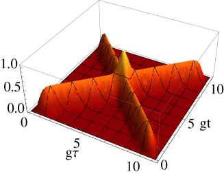
Figure 2: CPF correlation $C_{pf}(t,\tau)$ [Eq. (23)] as a function of both measurements times. The parameters are the same than in the previous figure. The behavior is periodic in both measurement time-intervals, $t$ and $\tau$. For increasing number of bath spins, $N\rightarrow\infty,$ the location of the central peak diverges.

Taking the scaling defined in Eq. (25), in Fig. 1 we plot the system coherence behaviors between consecutive measurements, $c_{t}$ [Eq. (18)] and $c_{t,\tau}^{yx}$ [Eq. (20)]. Both objects are very well fitted by Eqs. (26) and (27) respectively. On the other hand, we note that in general $c_{t,\tau}^{yx},$ as a function of $\tau,$ may develops strong departures with respect to $c_{t}.$ This feature depends on the product of outcomes $yx$ and is induced by the measurements back action that lead to different “initial” bath states, Eqs. (9) and (13) respectively. This property in turn lead to strong non-Markovian effects, whose presence can also be shown through the CPF correlation.

From Eqs. (23) and (26) $[f(t)\simeq\exp[-2(gt)^{2}],$ it follows the approximation

$$C_{pf}(t,\tau)\simeq\frac{e^{-2g^{2}(t+\tau)^{2}}+e^{-2g^{2}(t-\tau)^{2}}}{2}-e^{-2g^{2}(t^{2}+\tau^{2})}.$$ (28)

For increasing number of spins $N,$ this expression provides a very well fitting of Eq. (23). In Fig. 1(b), we plot the correlation for equal times, $C_{pf}(t,t).$ After a transient, it reaches a plateau regime, $C_{pf}(t,t)=1/2.$ This is the expected behavior when $N\rightarrow\infty.$ In fact, the correlation of the spin bath does not decay in time PRL . On the other hand, for finite $N$ recursive time behaviors are expected. This property is clear seen in Fig. 2, where as in Fig. 1 we taken $N=50.$ Due to the natural recurrence time of the total unitary dynamics, the temporal behavior is periodic in both measurement times (not shown). Consistently, the localization of the central peak (around $gt=g\tau\simeq 5.5)$ goes to infinity for increasing $N.$

IV Hamiltonian noise models

The spin bath model [Eq. (4)] has not a natural Markovian limit. In fact, the reservoir correlation does not decay in time. In solid state environments extra degrees of freedom coupled to the spin variables induce this feature. A simple way of representing this situation is to approximate the spin bath and “its environment” by a classical colored noise anderson . Thus, it is considered the stochastic Hamiltonian evolution

$$\frac{d}{dt}\rho_{t}^{st}=-i\xi(t)[\sigma_{\hat{z}},\rho_{t}^{st}],$$ (29)

where the system state $\rho_{t}$ follows by averaging $\rho_{t}^{st}$ over realizations of the real noise $\xi_{t},$ $\rho_{t}=\overline{\rho_{t}^{st}}$ GaussianNoise , which is denoted with the overbar symbol.

For simplicity, we only consider pure initial conditions. Hence, the problem can be studied through a stochastic wave vector, $\rho_{t}^{st}=|\psi_{t}\rangle\langle\psi_{t}|,$ whose evolution is

$$\frac{d}{dt}|\psi_{t}\rangle=-i\xi(t)\sigma_{\hat{z}}|\psi_{t}\rangle.$$ (30)

Taking the initial state $|\psi_{0}\rangle=a|+\rangle+b|-\rangle,$ which is uncorrelated from the noise realizations, the stochastic wave vector reads

$$|\psi_{t}\rangle=e^{-i\int_{0}^{t}dt^{\prime}\xi(t^{\prime})}a|+\rangle+e^{+i\int_{0}^{t}dt^{\prime}\xi(t^{\prime})}b|-\rangle.$$ (31)

This stochastic dynamics replaces the bipartite description given by Eq. (6).

Memory effects induced by the noise $\xi(t)$ can be studied through the measurement scheme associated to the CPF correlation. Similarly to the spin bath model, here the three successive measurements are chosen as projective ones, being performed in $\hat{x}$-direction (in the qubit Bloch sphere). The outcomes of each measurement are $x=\pm 1,$ $y=\pm 1,$ and $z=\pm 1,$ with measurement operators $\{\Omega_{x}\}=\{\Omega_{y}\}=\{\Omega_{z}\}=\{\Pi_{\hat{x}=\pm 1}\},$ where $\Pi_{\hat{x}=\pm 1}=|\hat{x}_{\pm}\rangle\langle\hat{x}_{\pm}|,$ with $|\hat{x}_{\pm}\rangle=(|+\rangle\pm|-\rangle)/\sqrt{2}.$ The system initial condition is taken as $|\psi_{0}\rangle=|+\rangle,$ which in turn is statistically independent of the noise.

IV.1 Conditional probabilities

The following calculations are performed by taking into account a particular noise realization. After the first $x$-measurement, the system state suffer the transformation $|\psi_{0}\rangle\rightarrow|\psi_{0}^{x}\rangle=\Pi_{\hat{x}=x}|\psi_{0}\rangle/\sqrt{\langle\psi_{0}|\Pi_{\hat{x}=x}|\psi_{0}\rangle},$ delivering

$$|\psi_{0}^{x}\rangle=\frac{|+\rangle+x|-\rangle}{\sqrt{2}},$$ (32)

where $x=\pm 1$ is the outcome of the measurement. The probability of both options is $P_{st}(x)=\langle\psi_{0}|\Pi_{\hat{x}=x}|\psi_{0}\rangle=1/2.$

In the next step, during a time interval $t$ the system evolves following the dynamics (31),

$$|\psi_{t}^{x}\rangle=\frac{1}{\sqrt{2}}\Big{[}e^{-i\int_{0}^{t}dt^{\prime}\xi(t^{\prime})}|+\rangle+e^{+i\int_{0}^{t}dt^{\prime}\xi(t^{\prime})}x|-\rangle\Big{]}.$$ (33)

The probability for the second measurement outcomes $y=\pm 1$ follow from $P_{st}(y|x)=\langle\psi_{t}^{x}|\Pi_{\hat{x}=y}|\psi_{t}^{x}\rangle,$ which then reads $P_{st}(y|x)=(1+yx\mathrm{Re}[\exp[-2i\int_{0}^{t}dt^{\prime}\xi(t^{\prime})]])/2.$ Clearly, this object is random and depends on each particular noise realization. The joint probability distribution $P_{st}(y,x)=P_{st}(y|x)P_{st}(x),$ is given by

$$P_{st}(y,x)=\frac{1}{4}(1+yx\mathrm{Re}[e^{-2i\int_{0}^{t}dt^{\prime}\xi(t^{\prime})}]),$$ (34)

which in turn implies, $P_{st}(y)=\sum_{x=\pm 1}P_{st}(y,x)=1/2.$ Thus, the retrodicted probability $P_{st}(x|y)=P_{st}(y,x)/P_{st}(y)$ can be written as

$$P_{st}(x|y)=\frac{1}{2}(1+yx\mathrm{Re}[e^{-2i\int_{0}^{t}dt^{\prime}\xi(t^{\prime})}]).$$ (35)

After the second $y$-measurement, the wave vector collapses as $|\psi_{t}^{x}\rangle\rightarrow|\psi_{t}^{yx}\rangle=\Pi_{\hat{x}=y}|\psi_{t}^{x}\rangle/\sqrt{\langle\psi_{t}^{x}|\Pi_{\hat{x}=y}|\psi_{t}^{x}\rangle},$ delivering

$$|\psi_{t}^{yx}\rangle=\frac{|+\rangle+y|-\rangle}{\sqrt{2}}.$$ (36)

Notice that this state only depend on the last outcome $y,$ being independent of the previous outcome $x.$ In addition it does not depend of the measurement time $t,$ neither on the particular noise realization.

In the next step, the system evolves with the stochastic unitary evolution (31) during a time interval $\tau,$ $|\psi_{t}^{yx}\rangle\rightarrow|\psi_{t+\tau}^{yx}\rangle.$ Hence,

$$|\psi_{t+\tau}^{yx}\rangle=\frac{1}{\sqrt{2}}\Big{[}e^{-i\int_{t}^{t+\tau}dt^{\prime}\xi(t^{\prime})}|+\rangle+e^{+i\int_{t}^{t+\tau}dt^{\prime}\xi(t^{\prime})}y|-\rangle\Big{]}.$$ (37)

The probability for the third $z$-measurement is $P_{st}(z|y,x)=\langle\psi_{t+\tau}^{yx}|\Pi_{\hat{x}=z}|\psi_{t+\tau}^{yx}\rangle,$

$$P_{st}(z|y,x)=\frac{1}{2}(1+zy\mathrm{Re}[e^{-2i\int_{t}^{t+\tau}dt^{\prime}\xi(t^{\prime})}]).$$ (38)

We notice that the conditional probabilities (35) and (38) depend on each particular noise realization in the intervals $(0,t)$ and $(t,t+\tau).$

IV.2 Dynamics between consecutive measurements

The dynamics between consecutive measurements can be obtained by averaging over noise realizations. After the first $x$-measurement and before the second $y$-measurement, the system state follows as $\rho_{t}^{x}=\overline{|\psi_{t}^{x}\rangle\langle\psi_{t}^{x}|},$ where $|\psi_{t}^{x}\rangle$ is given by Eq. (33). We get,

$$\rho_{t}^{x}=\frac{1}{2}\left(\begin{array}[]{cc}1&xc_{t}\\ xc_{t}^{\ast}&1\end{array}\right),$$ (39)

where the coherence behavior is given by

$$c_{t}=\overline{c_{st}(t)}\equiv\overline{\exp\Big{[}-2i\int_{0}^{t}dt^{\prime}\xi(t^{\prime})\Big{]}}.$$ (40)

Similarly to the quantum spin bath model, only the system coherences are affected.

After the second $y$-measurement and before the third $z$-measurement, the system state follows as $\rho_{t,\tau}^{yx}=\left.\overline{|\psi_{t+\tau}^{yx}\rangle\langle\psi_{t+\tau}^{yx}|}\right|_{yx},$ where $|\psi_{t+\tau}^{yx}\rangle$ is given by Eq. (37). We get,

$$\rho_{t,\tau}^{yx}=\frac{1}{2}\left(\begin{array}[]{cc}1&yc_{t,\tau}^{yx}\\ yc_{t,\tau}^{yx\ast}&1\end{array}\right),$$ (41)

where $c_{t,\tau}^{yx}$ is given by

$$c_{t,\tau}^{yx}=\left.\overline{c_{st}(t,\tau)}\right|_{yx}\equiv\left.\overline{\exp\Big{[}-2i\int_{t}^{t+\tau}dt^{\prime}\xi(t^{\prime})\Big{]}}\right|_{yx}.$$ (42)

In contrast with Eq. (40), in the previous expression the classical average (denoted as $\left.\overline{\mathcal{F}[\xi]}\right|_{yx},$ where $\mathcal{F}[\xi]$ is a functional of the noise) is restricted (conditioned) to the occurrence of the previous $x$ and $y$ measurement outcomes. The probability $P([\xi]|y,x)$ of a noise realization conditioned on these outcomes, from Bayes rule, is

$$P([\xi]|y,x)=\frac{P_{st}(y,x)P([\xi])}{\overline{P_{st}(y,x)}}.$$ (43)

Here, $P([\xi])$ is the unconditional probability of a noise realization. Furthermore, $P_{st}(y,x)$ is the joint probability of $y$ and $x$ outcomes conditioned to a given noise realization. Thus, it is given by Eq. (34). For an arbitrary noise functional, the conditional average $\left.\overline{\mathcal{F}[\xi]}\right|_{yx}$ can then be written as

$$\left.\overline{\mathcal{F}[\xi]}\right|_{yx}=\overline{\mathcal{F}[\xi]P([\xi]|y,x)}=\frac{\overline{\mathcal{F}[\xi]P_{st}(y,x)}}{\overline{P_{st}(y,x)}}.$$ (44)

Applying this result to Eq. (42), we get the final expression

$$c_{t,\tau}^{yx}=\overline{\frac{c_{st}(t,\tau)(1+yx\mathrm{Re}[c_{st}(t)])}{1+yx\overline{\mathrm{Re}[c_{st}(t)]}}},$$ (45)

which is defined in terms of unconditional classical ensemble averages.

We notice that $c_{t,\tau}^{yx}\neq c_{t}.$ This change of dynamics follows from a measurement back action on the (average) environmental influence. In fact, this feature emerges from conditioning the classical noise average to the occurrence of previous quantum measurement outcomes. The different coherence behaviors indicates the non-Markovian property of the system dynamics. In fact, Eqs. (40) and (45) are the analog of Eqs. (18) and (20), which correspond to the quantum spin environment.

IV.3 CPF correlation

The conditional probabilities $P_{st}(x|y)$ [Eq. (35)] and $P_{st}(z|y,x)$ [Eq. (38)] relies on quantum measurement theory. They were calculated taking into account a single noise realization. The probability $P(z,x|y),$ which defines the CPF correlation (3), describes the statistics for an ensemble of (conditional) measurement results. Given its conditional character, it can be written as

$$P(z,x|y)=\overline{P_{st}(z,x}|y)=\overline{P_{st}(z|y,x)P_{st}(x|y)}|_{y},$$ (46)

where the (classical noise) average is conditioned to the occurrence of a particular $y$-outcome. This average can be performed with the conditional probability $P([\xi]|y)=P_{st}(y)P([\xi])/\overline{P_{st}(y)},$ where $P_{st}(y)$ is the probability of obtaining a $y$-outcome for a given noise realization. Nevertheless, for the chosen initial conditions $P_{st}(y)=\sum_{x=\pm 1}P_{st}(y,x)=1/2$ [see Eq. (34)]. Thus, $P([\xi]|y)=P([\xi]),$ which implies that, for the chosen initial conditions, the noise average in Eq. (46) can be taken as an unconditional one, $P(z,x|y)=\overline{P_{st}(z|y,x)P_{st}(x|y)}.$ Using this result, from Eqs. (35) and (38) it is possible to obtain

$$P(z,x|y)=\frac{1}{4}\Big{[}1+xyf(t)+zyf^{\prime}(\tau)+zxf(t,\tau)\Big{]}.$$ (47)

The auxiliary functions are

$$f(t)=\overline{\mathrm{Re}[c_{st}(t)]}=\overline{\mathrm{Re}\left[e^{-2i\int_{0}^{t}dt^{\prime}\xi(t^{\prime})}\right]}.$$ (48)

Thus, $f(t)=\mathrm{Re}[c_{t}]$ [Eq. (40)]. Furthermore,

$$f^{\prime}(\tau)=\overline{\mathrm{Re}[c_{st}(t,\tau)]}=\overline{\mathrm{Re}\left[e^{-2i\int_{t}^{t+\tau}dt^{\prime}\xi(t^{\prime})}\right]}.$$ (49)

For stationary noises vanKampen this function does not depend on the time $t.$ In fact, stationarity implies $f^{\prime}(\tau)=f(\tau).$ Finally,

$$f(t,\tau)=\overline{\mathrm{Re}[c_{st}(t)]\mathrm{Re}[c_{st}(t,\tau)]},$$ (50)

which explicitly reads

$$f(t,\tau)=\overline{\mathrm{Re}\left[e^{-2i\int_{0}^{t}dt^{\prime}\xi(t^{\prime})}\right]\mathrm{Re}\left[e^{-2i\int_{t}^{t+\tau}dt^{\prime}\xi(t^{\prime})}\right]}.$$ (51)

From Eq. (47), using that $O_{z}=z,$ $O_{x}=x,$ the conditional averages read $\overline{\langle O_{z}\rangle_{y}}=yf(\tau),$ $\overline{\langle O_{x}\rangle_{y}}=yf(t),$ and $\overline{\langle O_{z}O_{x}\rangle_{y}}=f(t,\tau).$ The CPF correlation, $C_{pf}(t,\tau)=\overline{\langle O_{z}O_{x}\rangle_{y}}-\overline{\langle O_{z}\rangle_{y}}\ \overline{\langle O_{x}\rangle_{y}},$ becomes

$$C_{pf}(t,\tau)=f(t,\tau)-f(t)f(\tau).$$ (52)

These expressions recover the exact results presented in Ref. PRL .

Taking into account the expressions (48) and (51), we realize that $C_{pf}(t,\tau)$ corresponds to the centered correlation of the real part of the phase terms $\exp[-2i\int_{0}^{t}dt^{\prime}\xi(t^{\prime})]$ and $\exp[-2i\int_{t}^{t+\tau}dt^{\prime}\xi(t^{\prime})],$ which in turn correspond to the (stochastic) coherence decay behaviors in the intervals $(0,t)$ and $(t,t+\tau),$ respectively.

The exact result (52) can be evaluated for arbitrary (stationary) noises. The (real) functions $f(t)$ and $f(t,\tau)$ also determine the system dynamics between consecutive measurements, Eqs. (40) and (45). In fact, for a stationary noise with a vanishing mean value, $\overline{\xi(t)}=0,$ it follows

$$c_{t}=f(t),\ \ \ \ \ \ \ \ \ \ \ \ c_{t,\tau}^{yx}=\frac{f(\tau)+yxf(t,\tau)}{1+yxf(t)}.$$ (53)

IV.4 Gaussian Noise

Gaussian fluctuations arise naturally in different physical situations such as for example in solid state environments anderson ; abragam . For this statistics, the calculation of the functions $f(t)$ and $f(t,\tau)$ [Eqs. (48) and (51)] can be performed in different alternative ways. Here, they are determine through the characteristic noise functional vanKampen ,

$$G[k]=\overline{\exp\left[i\int_{0}^{\infty}k(t^{\prime})\xi(t^{\prime})dt^{\prime}\right]},$$ (54)

which depends on an arbitrary test function $k(t).$ For a Gaussian noise with null average, $\overline{\xi(t)}=0,$ it reads vanKampen

$$G[k]=\exp\Big{[}-\frac{1}{2}\int_{0}^{\infty}dt_{2}\int_{0}^{\infty}dt_{1}k(t_{2})k(t_{1})\chi(t_{2},t_{1})\Big{]},$$ (55)

where $\chi(t_{2},t_{1})\equiv\overline{\xi(t_{2})\xi(t_{1})}=\chi(|t_{2}-t_{1}|)$ is the noise correlation. The last equality is valid for stationary noises.

After giving an explicit noise correlation, the averages (48) and (51) follows by writing $\mathrm{Re}[a]=(a+a^{\ast})/2,$ and by taking an adequate set of test functions. For example, $\overline{\exp i\int_{0}^{t}\xi(t^{\prime})dt^{\prime}}$ follows from $G[k]$ with $k(t^{\prime})=\theta(t-t^{\prime}),$ where $\theta(x)$ is the step function, and performing the corresponding time integrals. Similarly, the calculus of $\overline{\exp i[\int_{t}^{t+\tau}\xi(t^{\prime})dt^{\prime}\pm\int_{0}^{t}\xi(t^{\prime})dt^{\prime}]}$ is obtained with $k(t^{\prime})=\theta(t+\tau-t^{\prime})\theta(t^{\prime}-t)\pm\theta(t-t^{\prime}).$

IV.4.1 White noise

For a white noise, $\chi(t_{2},t_{1})=\gamma_{w}\delta(t_{2}-t_{1}),$ it follows

$$f(t)=\exp[-2\gamma_{w}t],\ \ \ \ \ \ \ \ \ f(t,\tau)=f(t)f(\tau).$$ (56)

Hence, a Markovian limit is achieved,

$$c_{\tau}=c_{t,\tau}^{yx}=f(\tau),\ \ \ \ \ \ C_{pf}(t,\tau)=0.$$ (57)

In fact, here the system dynamics between consecutive measurement events do not depend on the measurement outcomes and are the same. Consistently, the CPF correlation vanishes. Furthermore, both intermediate dynamics [Eqs. (39) and (41)] obey a (dephasing) Lindblad evolution,

$$\frac{d\rho_{t}}{dt}=\frac{1}{2}\gamma(t)(\sigma_{\hat{z}}\rho_{t}\sigma_{\hat{z}}-\rho_{t}),$$ (58)

where the time dependent rate is determined by the coherence behavior

$$\gamma(t)=-\frac{1}{\langle+|\rho_{t}|-\rangle}\frac{d}{dt}\langle+|\rho_{t}|-\rangle.$$ (59)

Thus, in both cases $\gamma(t)=2\gamma_{w}.$

IV.4.2 Infinite correlation-time

This case corresponds to a noise correlation that does not decay in time, $\chi(t_{2},t_{1})=g^{2}.$ We obtain

$$f(t)=\exp[-2(gt)^{2}],\ \ \ \ \ f(t,\tau)=f(t+\tau)+f(t-\tau).$$ (60)

This decay behavior recovers the (asymptotic in $N)$ dynamics induced by the spin bath model when developing pure Gaussian decay behaviors. Thus, the exact expression for the coherences $c_{\tau}$ and $c_{t,\tau}^{yx}$ [Eq. (53)] are given by Eqs. (26) and (27) respectively. The CPF correlation then correspond to Eq. (28). Between the first two measurements [Eq. (39)], the system evolution is given by Eq. (58) with $\gamma(t)=4g^{2}t>0.$ A more complex expression (which depends on the product $yx$ of measurement outcomes) describes the rate for the second evolution [Eq. (41)].

IV.4.3 Exponential correlation

For an exponential correlation

$$\chi(t_{2},t_{1})=g^{2}\exp[-|t_{2}-t_{1}|/\tau_{c}],$$ (61)

where the parameter $\tau_{c}$ gives the characteristic correlation-time of the noise fluctuations, it follows

$$f(t)=\exp\Big{\{}-4(\tau_{c}g)^{2}[t/\tau_{c}-(1-e^{-t/\tau_{c}})]\Big{\}}.$$ (62)

The function (51) reads

$$f(t,\tau)=f(t)f(\tau)\cosh[\varphi(t,\tau)],$$ (63)

where the auxiliary function is

$$\varphi(t,\tau)\equiv 4(\tau_{c}g)^{2}(1-e^{-t/\tau_{c}})(1-e^{-\tau/\tau_{c}}).$$ (64)

In the limit $\tau_{c}\rightarrow\infty,$ these expressions consistently give the infinite correlation limit (60). On the other hand, taking $\gamma_{w}/2=g^{2}\tau_{c}$ as a constant parameter, in the limit $\tau_{c}\rightarrow 0,$ the Markovian regime (56) is recovered.

In Fig. 3 we plot the coherence decay $c_{\tau}$ and $c_{t,\tau}^{yx}$ [Eq. (53)] between consecutive measurement events. For larger correlations times $(g\tau_{c}=100),$ the behavior is similar to that of the quantum spin bath (see Fig. 1). On the other hand, for smaller correlation times $(g\tau_{c}=5),$ the measurement back action on the coherence behavior is diminished. In fact, the difference between both dynamics disappear in a white noise limit. The dynamics between the first two measurement is given by the Lindblad evolution (58) with $\gamma(t)=4g^{2}\tau_{c}(1-e^{-t/\tau_{c}})>0,$ while a more complex expression describes the rate for the second evolution [Eq. (41)].

In Fig. 4, for the same correlation time $(g\tau_{c}=5),$ it is plotted the CPF correlation [Eq. (52)]. Its maximal amplitude (central peak) diminishes when $\tau_{c}$ diminishes (compare with Fig. 2, which can be read as the $\tau_{c}\rightarrow\infty$ limit). Furthermore, as the Markovian limit is being approached, $C_{pf}(t,\tau)$ is not null only at short times.

In order to visualize the transition between Markovian and non-Markovian regimes, in Fig. 5(a) we plot the coherence behavior $c_{\tau}$ [Eq. (53)]. Different values of the correlation $\tau_{c}$ are chosen while the parameter $\gamma_{w}/2=g^{2}\tau_{c}$ remains constant. A transition between exponential and Gaussian behaviors is clearly seen when increasing the correlation time $\tau_{c}.$ In Fig. 5(b) we also plot the CPF correlation for a set of different correlation times. For increasing $\tau_{c}$ the limit (28) is recovered, while for decreasing $\tau_{c}$ the CPF correlation approaches the Markovian limit (57).

Figure 3: Coherence decay behaviors $c_{\tau}$ and $c_{t,\tau}^{yx}$ between consecutive measurements [Eq. (53)] for the Gaussian stochastic Hamiltonian model with exponential correlation (61) for different correlation times $\tau_{c},$ (a) $g\tau_{c}=100,$ (b) $g\tau_{c}=5.$ In both cases $gt=1.5.$

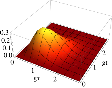
Figure 4: CPF correlation [Eq. (52) jointly with Eqs. (62) and (63)] for the Gaussian stochastic Hamiltonian model with exponential correlation (61) with parameters $g\tau_{c}=5.$

Figure 5: (a) System coherence $c_{\tau}$ [Eqs. (53) and (62)] for the Gaussian stochastic Hamiltonian model with exponential correlation (61) for different correlation times $\tau_{c},$ where $\gamma_{w}/2=g^{2}\tau_{c}.$ (b) CPF correlation (52) for equal times, $C_{pf}(\tau,\tau),$ for different correlation times $\tau_{c}.$

V Non-Markovian Dephasing Lindblad evolutions

Lindblad dynamics [like Eq. (58)] with positive rates are associated to a Markovian regime BreuerReview ; plenioReview . In the present scheme quantum Markovianity does not rely on Lindblad theory. It is defined by a vanishing CPF correlation. If both evolutions between consecutive measurement events are defined by the same Lindblad equation the CPF correlation vanishes. In the previous Hamiltonian model this situation arises when the noise is a delta correlated one.

In this section we show that even when the evolution between the first and second measurement events is given by a time-independent Lindblad equation, the posterior evolution (between the second and third measurements) may change, implying a non-vanishing CPF correlation. Thus, the original Lindblad equation cannot be associated to a Markovian dynamics. This unusual non-Markovian effect emerges when the underlying parameters of the studied models become Lorentzian random variables vanKampen ; caceres .

V.1 Spin environment with random coupling

In solid state environments the couplings $\{g_{k}\}$ in the spin bath model (4) may become random variables Paz . This feature may represents, for example, distance-dependent system-bath interactions modulated by the random location of each spin of the environment abragam . Independently of its physical origin, the description of a random coupling model follows from the results of Sec. II after averaging over the distribution of the set $\{g_{k}\}:$

$$\mathbf{c}_{t}\equiv\overline{c_{t}},\ \ \ \ \ \ \mathbf{c}_{t,\tau}^{yx}\equiv\left.\overline{c_{t,\tau}^{yx}}\right|_{yx},\ \ \ \mathbf{C}_{pf}(t,\tau)\equiv\left.\overline{C_{pf}(t,\tau)}\right|_{y}.$$ (65)

In these expressions bold letters denote averaged quantities. The (random) objects are defined by Eqs. (18), (20), and (23), evaluated in a particular realization of the set $\{g_{k}\}.$ The overbar denotes average over their probability distributions.

The average that gives $\mathbf{c}_{t}$ is an unconditional one. Nevertheless, for$\ \mathbf{c}_{t,\tau}^{yx}$ the classical average is conditioned to the occurrence of $y$ and $x$ outcomes. Similarly to Eq. (43), from Bayes rule this conditional average is defined by the distribution

$$P(\{g_{k}\}|y,x)=\frac{P(y,x)P(\{g_{k}\})}{\overline{P(y,x)}},$$ (66)

where $P(\{g_{k}\})$ is the (unconditional) probability distribution of the coupling constants, while $P(y,x)$ is given by Eq. (11) evaluated in a particular realization of the set $\{g_{k}\}.$ Thus, from Eq. (20), the coherence behavior between the first two ($x$ and $y$) measurements is

$$\mathbf{c}_{t,\tau}^{yx}=\overline{\frac{c_{\tau}+yx(c_{t+\tau}+c_{t-\tau}^{\ast})/2}{1+yx\overline{(c_{t}+c_{t}^{\ast})/2}}},$$ (67)

which is written in terms of unconditional averages.  

The correlation $\mathbf{C}_{pf}(t,\tau)$ [Eq. (65)] is defined by a classical average conditioned to the occurrence of a particular $y$-outcome. Nevertheless, due to the chosen initial conditions, similarly to the average in Eq. (46), it can be taken as an unconditional one. Thus, $\mathbf{C}_{pf}(t,\tau)=\overline{C_{pf}(t,\tau)}.$

Lorentz probability distribution

The coupling $\{g_{k}\}$ are taken as independent identical random variables, with the scaling

$$g_{k}=\frac{1}{N}\tilde{g}.$$ (68)

The probability density of the random variable $\tilde{g}$ is a Lorentzian one,

$$P(\tilde{g})=\frac{\gamma/2}{\pi[(\tilde{g}-\omega/2)^{2}+(\gamma/2)^{2}]},$$ (69)

where $\gamma$ and $\omega$ are free parameters. Denoting with an overbar the average over $\tilde{g},$ it follows the relation caceres

$$\overline{\exp(+2i\tilde{g}t)}=\int_{-\infty}^{+\infty}d\tilde{g}P(\tilde{g})e^{+2i\tilde{g}t}=\exp(i\omega t)\exp(-\gamma|t|).$$ (70)

Thus, random phases with a Lorentzian distribution leads to exponential decay behaviors.

Assuming that all spin of the reservoir begin in the same state, $\alpha_{k}=\alpha,$ $\beta_{k}=\beta,$ with $|\alpha|^{2}+|\beta|^{2}=1,$ from Eq. (18) the average coherence behavior $\mathbf{c}_{t}$ is given by

$$\mathbf{c}_{t}=\overline{c_{t}}=e^{-\gamma|t|}(|\alpha|^{2}e^{+i\omega t/N}+|\beta|^{2}e^{-i\omega t/N})^{N}.$$ (71)

Hence, and exponential decay behavior is valid for arbitrary $N.$ Furthermore, for $N\gg 1,$ it can be approximated as $\mathbf{c}_{t}\simeq e^{-\gamma|t|}\exp[i(|\alpha|^{2}-|\beta|^{2})\omega t].$ If $|\alpha|^{2}=|\beta|^{2}=1/2,$ or alternatively taking $\omega=0,$ the induced complex phase vanishes. Thus, from Eq. (71) it follows the pure exponential decay behavior

$$\mathbf{c}_{t}=\exp[-\gamma|t|].$$ (72)

Similarly, from Eq. (67) it follows the exact result

$$\mathbf{c}_{t,\tau}^{yx}=\frac{e^{-\gamma|\tau|}+yx(e^{-\gamma|t+\tau|}+e^{-\gamma|t-\tau|})}{1+yxe^{-\gamma|t|}}.$$ (73)

Figure 6: (a) System coherences $\mathbf{c}_{t}$ [Eq. (72)] and $\mathbf{c}_{t,\tau}^{yx}$ [Eq. (73)] for the spin bath model with Lorentzian distributed coupling. (b) CPF correlation (74) for equal times, $\mathbf{C}_{pf}(\tau,\tau).$ In both figures, the random coupling are given by the scaling Eq. (68), while the average coupling is null, $\omega=0$ [Eq. (69)], and $N=50.$ The system and bath initial conditions are the same than in Fig. 1.

The exponential behavior (72) implies that between the first two measurements the system dynamics is given by a dephasing Lindblad equation with a time-independent rate [Eq. (58) with $\gamma(t)=\gamma$]. Nevertheless, the second $y$-measurement induces a posterior change of system behavior [see Eqs. (9) and (13)]. The change $\mathbf{c}_{t}\rightarrow\mathbf{c}_{t,\tau}^{yx},$ in spite of the former pure exponential behavior, indicates that the dynamics is non-Markovian. Consequently, a Linblad dynamics does not guarantee quantum Markovianity. In Fig. 6(a) we show the behavior of both $\mathbf{c}_{t}$ and $\mathbf{c}_{t,\tau}^{yx},$ which is given by the previous two expressions. $\mathbf{c}_{t,\tau}^{yx}$ develops a non-differentiable time-behavior which is induced by the Lorentzian coupling statistics.

The non-Markovian property of the system dynamics can also be shown through the CPF correlation. From Eqs. (23) and (65) [with $\mathbf{C}_{pf}(t,\tau)=\overline{C_{pf}(t,\tau)}]$ straightforwardly it follows the exact expression

$$\mathbf{C}_{pf}(t,\tau)=\frac{e^{-\gamma|t+\tau|}+e^{-\gamma|t-\tau|}}{2}-e^{-\gamma(|t|+|\tau|)},$$ (74)

which certainly is not null.

In Fig. 6(b) we plot $\mathbf{C}_{pf}(t,\tau)$ for equal times intervals while in Fig. 7 we plot its dependence on both times. In contrast to Fig. 2, due to the randomness of the coupling coefficients, the time behavior is not periodic in time. Furthermore, the asymptotic behavior $\lim_{t\rightarrow\infty}C_{pf}(t,t)=1/2$ again is related to an infinite environment correlation-time.

The dynamics characterized previously demonstrates that a Lindblad equation may arises even when the Born-Markov approximation does not applies. Notice that the non-Markovian character of the evolution can only be detected through extra information that is not encoded in the density matrix dynamics corresponding to the time interval $(0,t).$

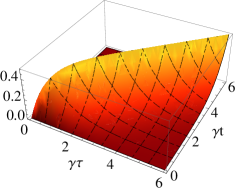
Figure 7: CPF correlation $\mathbf{C}_{pf}(t,\tau)$ [Eq. (74)] for the spin bath model with Lorentzian coupling constants. The parameters are the same than in the previous figure.

V.2 Random frequency models

Instead of a time-dependent stochastic noise one can consider a random frequency model, that is, Eq. (29) under the replacement $\xi(t)\rightarrow\tilde{g},$

$$\frac{d}{dt}\rho_{t}^{st}=-i\tilde{g}[\sigma_{\hat{z}},\rho_{t}^{st}],$$ (75)

where $\tilde{g}$ is a (time-independent) random variable with probability density $P(\tilde{g}).$ The infinite correlation limit of the Gaussian noise [Eq. (55)] can be read in this way, where $P(\tilde{g})$ is a Gaussian distribution. On the other hand, we notice that the evolution (75) corresponds to a particular case of a (quantum-classical) generalized Lindblad equation LindbladRate .

All calculations performed in Sec. IV applies to the present model after replacing $\xi(t)\rightarrow\tilde{g}.$ The functions $f(t)$ and $f^{\prime}(\tau)$ [Eqs. (48) and (49)] become

$$f(t)=\frac{\overline{e^{+2i\tilde{g}t}+e^{-2i\tilde{g}t}}}{2},\ \ \ \ f^{\prime}(\tau)=\frac{\overline{e^{+2i\tilde{g}\tau}+e^{-2i\tilde{g}\tau}}}{2},$$ (76)

where the overbar here denotes average with the distribution $P(\tilde{g}).$ Eq. (51) becomes

$$f(t,\tau)=\frac{\overline{(e^{+2i\tilde{g}t}+e^{-2i\tilde{g}t})(e^{+2i\tilde{g}\tau}+e^{-2i\tilde{g}\tau})}}{4}.$$ (77)

Lorentzian random frequencies

Similarly to the spin bath model, here we chose a Lorentzian distribution (69) for $\tilde{g}.$ Taking $\omega=0,$ from Eq. (70) it follows

$$f(t)=\exp[-\gamma|t|],\ \ \ \ f^{\prime}(\tau)=\exp[-\gamma|\tau|],$$ (78)

and similarly

$$f(t,\tau)=\frac{\exp[-\gamma|t+\tau|]+\exp[-\gamma|t-\tau|]}{2}.$$ (79)

With these expressions at hand it is simple to realize that $c_{t}$ and $c_{t,\tau}^{yx}$ [Eq.(53)] are given by Eqs. (72) and (73) respectively. Furthermore, the CPF correlation $C_{pf}(t,\tau)$ [Eq. (52)] is given by Eq. (74). Therefore, the random frequency model leads to the same results and expressions than the spin bath model with Lorentzian random coefficients. This simplified model [Eq. (75)] also demonstrate that a Lindblad equation may relies on strong system-environment correlations.

VI Conclusions

Similarly to classical systems, quantum non-Markovian effects can be studied through a CPF correlation. Its definition relies on three quantum measurements performed successively over the system of interest. We characterized the CPF correlation for a qubit system whose non-Markovian dynamics is induced by different dephasing mechanisms. Over the basis of standard quantum measurement theory, exact expressions were found for a quantum spin environment as well as for stochastic Hamiltonians models.

The present analysis allowed us to relate the presence of memory effects, indicated by a nonvanishing CPF correlation, with a measurement back action that change the system dynamics between consecutive measurement events. In fact, in a Markovian limit, defined by a vanishing CPF correlation, this dynamical change is absent. For the Hamiltonian noise model Markovianity emerges in a white noise limit.

Taking the underlying parameters of the models as random variables with a Lorentzian probability density, the former system evolution between the first two measurements is given a dephasing Lindblad equation with a time-independent rate. In spite of this feature, the posterior system evolution, between the second and third measurements, is different from the former one. This unexpected (non-Markovian) property demonstrates that Lindblad equations may emerge even when the system and the environment are highly correlated. Quantum non-Markovian measures based solely on the system density matrix evolution are unable to detect these non-Markovian features.

References

- (1) N. G. van Kampen, Stochastic Processes in Physics and Chemistry, (North-Holland, Amsterdam, 1981).
- (2) H. P. Breuer and F. Petruccione, The theory of open quantum systems, (Oxford University Press, 2002).
- (3) I. de Vega and D. Alonso, Dynamics of non-Markovian open quantum systems, Rev. Mod. Phys. 89, 015001 (2017).
- (4) R. Alicki and K. Lendi, Quantum Dynamical Semigroups and Applications, Lect. Notes Phys. 717 (Springer, Berlin Heidelberg, 1987).
- (5) H. P. Breuer, E. M. Laine, J. Piilo, and V. Vacchini, Colloquium: Non-Markovian dynamics in open quantum systems, Rev. Mod. Phys. 88, 021002 (2016).
- (6) A. Rivas, S. F. Huelga, and M. B. Plenio, Quantum non-Markovianity: characterization, quantification and detection, Rep. Prog. Phys. 77, 094001 (2014).
- (7) H. P. Breuer, E. M. Laine, and J. Piilo, Measure for the Degree of Non-Markovian Behavior of Quantum Processes in Open Systems, Phys. Rev. Lett. 103, 210401 (2009).
- (8) M. M. Wolf, J. Eisert, T. S. Cubitt, and J. I. Cirac, Assessing Non-Markovian Quantum Dynamics, Phys. Rev. Lett. 101, 150402 (2008).
- (9) A. Rivas, S. F. Huelga, and M. B. Plenio, Entanglement and Non-Markovianity of Quantum Evolutions, Phys. Rev. Lett. 105, 050403 (2010).
- (10) D. Chruściński and S. Maniscalco, Degree of Non-Markovianity of Quantum Evolution, Phys. Rev. Lett. 112, 120404 (2014).
- (11) J. Bae and D. Chruściński, Operational Characterization of Divisibility of Dynamical Maps, Phys. rev. Lett. 117, 050403 (2016).
- (12) D. Chruściński, A. Kossakowski, and A. Rivas, Measures of non-Markovianity: Divisibility versus backflow of information, Phys. Rev. A 83, 052128 (2011).
- (13) B. Bylicka, M. Johansson, and A. Acín, Constructive Method for Detecting the Information Backflow of Non-Markovian Dynamics, Phys. Rev. Lett. 118, 120501 (2017).
- (14) P. Haikka, J. D. Cresser, and S. Maniscalco, Comparing different non-Markovianity measures in a driven qubit system, Phys. Rev. A 83, 012112 (2011). C. Addis, B. Bylicka, D. Chruściński, and S. Maniscalco, Comparative study of non-Markovianity measures in exactly solvable one- and two-qubit models, Phys. Rev. A 90, 052103 (2014).
- (15) M. J. W. Hall, J. D. Cresser, L. Li, and E. Andersson, Canonical form of master equations and characterization of non-Markovianity, Phys. Rev. A 89, 042120 (2014).
- (16) S. Lorenzo, F. Plastina, and M. Paternostro, Geometrical characterization of non-Markovianity, Phys. Rev. A 88, 020102(R) (2013).
- (17) X.-M. Lu, X. Wang, and C. P. Sun, Quantum Fisher information flow and non-Markovian processes of open systems, Phys. Rev. A 82, 042103 (2010).
- (18) S. Luo, S. Fu, and H. Song, Quantifying non-Markovianity via correlations, Phys. Rev. A 86, 044101 (2012).
- (19) F. F. Fanchini, G. Karpat, B. Çakmak, L. K. Castelano, G. H. Aguilar, O. Jiménez Farías, S. P. Walborn, P. H. Souto Ribeiro, and M. C. de Oliveira, Non-Markovianity through Accessible Information, Phys. Rev. Lett. 112, 210402 (2014).
- (20) A. K. Rajagopal, A. R. Usha Devi, and R. W. Rendell, Kraus representation of quantum evolution and fidelity as manifestations of Markovian and non-Markovian forms, Phys. Rev. A 82, 042107 (2010).
- (21) N. Megier, D. Chruściński, J. Piilo, and W. T. Strunz, Eternal non-Markovianity: from random unitary to Markov chain realisations, Sci. Rep. 7, 6379 (2017).
- (22) A. A. Budini, Maximally non-Markovian quantum dynamics without environment-to-system backflow of information, Phys. Rev. A 97, 052133 (2018).
- (23) F. A. Pollock, C. Rodríguez-Rosario, T. Frauenheim, M. Paternostro, and K. Modi, Operational Markov Condition for Quantum Processes, Phys. Rev. Lett. 120, 040405 (2018); F. A. Pollock, C. Rodríguez-Rosario, T. Frauenheim, M. Paternostro, and K. Modi, Non-Markovian quantum processes: Complete framework and efficient characterization, Phys. Rev. A 97, 012127 (2018).
- (24) A. A. Budini, Quantum Non-Markovian Processes Break Conditional Past-Future Independence, Phys. Rev. Lett. 121, 240401 (2018).
- (25) T. M. Cover and J. A. Thomas, Elements of Information Theory, (Wiley&Sons, New Jersey, 1991).
- (26) Y. Aharonov and L. Vaidman, Properties of a quantum system during the time interval between two measurements, Phys. Rev. A 41, 11 (1990); Y. Aharonov and L. Vaidman, Complete description of a quantum system at a given time, J. Phys. A: Math. Gen. 24, 2315 (1991).
- (27) D. Tan, S. J. Weber, I. Siddiqi, K. Mølmer, and K. W. Murch, Prediction and Retrodiction for a Continuously Monitored Superconducting Qubit, Phys. Rev. Lett. 114, 090403 (2015).
- (28) S. Gammelmark, B. Julsgaard, and K. Mølmer, Past Quantum States of a Monitored System, Phys. Rev. Lett. 111, 160401 (2013).
- (29) T. Rybarczyk, B. Peaudecerf, M. Penasa, S. Gerlich, B. Julsgaard, K. Mølmer, S. Gleyzes, M. Brune, J. M. Raimond, S. Haroche, and I. Dotsenko, Forward-backward analysis of the photon-number evolution in a cavity, Phys. Rev. A 91, 062116 (2015).
- (30) P. Campagne-Ibarcq, L. Bretheau, E. Flurin, A. Auffèves, F. Mallet, and B. Huard, Observing Interferences between Past and Future Quantum States in Resonance Fluorescence, Phys. Rev. Lett. 112, 180402 (2014).
- (31) N. Foroozani, M. Naghiloo, D. Tan, K. Mølmer and K. W. Murch, Correlations of the Time Dependent Signal and the State of a Continuously Monitored Quantum System, Phys. Rev. Lett. 116, 110401 (2016).
- (32) D. Tan, N. Foroozani, M. Naghiloo, A. H. Kiilerich, K. Mølmer, and K. W. Murch, Homodyne monitoring of postselected decay, Phys. Rev. A 96, 022104 (2017).
- (33) A. A. Budini, Entropic relations for retrodicted quantum measurements, Phys. Rev. A 97, 012132 (2018).
- (34) M. Tsang, Time-symmetric quantum theory of smoothing, Phys. Rev. Lett. 102, 250403 (2009); I. Guevara and H. Wiseman, Quantum State Smoothing, Phys. Rev. Lett. 115, 180407 (2015); A. A. Budini, Smoothed quantum-classical states in time-irreversible hybrid dynamics, Phys. Rev. A 96, 032118 (2017).
- (35) J. Dressel and A. N. Jordan, Quantum instruments as a foundation for both states and observables, Phys. Rev. A 88, 022107 (2013); L. P. García-Pintos and J. Dressel, Past observable dynamics of a continuously monitored qubit, Phys. Rev. A 96, 062110 (2017).
- (36) S. M. Barnett, D. T. Pegg, J. Jeffers, and O. Jedrkiewicz, Master equation for retrodiction of quantum communication signals, Phys. Rev. Lett. 86, 2455 (2001); D. T. Pegg, S. M. Barnett, and J. Jeffers, Quantum retrodiction in open systems, Phys. Rev. A 66, 022106 (2002); S. M. Barnett, D. T. Pegg, J. Jeffers, O. Jedrkiewicz, and R. Loudon, Retrodiction for quantum optical communications, Phys. Rev. A 62, 022313 (2000).
- (37) H. M. Wiseman and G. J. Milburn, Quantum Measurement and Control (Cambridge University press, 2010).
- (38) W. H. Zurek, Environment-induced superselection rules, Phys. Rev. D 26, 1862 (1982).
- (39) W. H. Zurek, Decoherence, einselection, and the quantum origins of the classical, Rev. Mod. Phys. 75, 715 (2003).
- (40) F. M. Cucchietti, J. P. Paz, and W. H. Zurek, Decoherence from spin environments, Phys. Rev. A 72, 052113 (2005).
- (41) H. M. Pastawski, P. R. Levstein, and G. Usaj, Quantum Dynamical Echoes in the Spin Diffusion in Mesoscopic Systems, Phys. Rev. Lett. 75, 4310 (1995); G. A. Álvarez, A. Ajoy, X. Peng, and D. Suter, Performance comparison of dynamical decoupling sequences for a qubit in a rapidly fluctuating spin bath, Phys. Rev. A 82, 042306 (2010); D. Bendersky, P. R. Zangara, and H. M. Pastawski, Fragility of superposition states evaluated by the Loschmidt echo, Phys. Rev. A 88, 032102 (2013).
- (42) P. W. Anderson and P. R. Weiss, Exchange Narrowing in Paramagnetic Resonance, Rev. Mod. Phys. 25, 269 (1953); P. T. Callaghan, Principles of Nuclear Magnetic Resonance Microscopy, (Clarendom Press, Oxford, 1991).
- (43) A. A. Budini, Quantum systems subject to the action of classical stochastic fields, Phys. Rev. A 64, 052110 (2001).
- (44) A. Abragam, The Principles of Nuclear Magnetism (Oxford University Press, Oxford, 1961); T. T. P. Cheung, Spin diffusion in NMR in solids, Phys. Rev. B 23, 1404 (1980).
- (45) M. O. Cáceres, Non-equilibrium Statistical Physics with Application to Disordered Systems (Springer, New York, 2017).
- (46) A. A. Budini, Random Lindblad equations from complex environments, Phys. Rev. E 72, 056106 (2005); A. A. Budini, Lindblad rate equations, Phys. Rev. A 74, 053815 (2006).