Zero-Shot Autonomous Vehicle Policy Transfer: From Simulation to Real-World via Adversarial Learning

Abstract

In this article, we demonstrate a zero-shot transfer of an autonomous driving policy from simulation to University of Delaware’s scaled smart city with adversarial multi-agent reinforcement learning, in which an adversary attempts to decrease the net reward by perturbing both the inputs and outputs of the autonomous vehicles during training. We train the autonomous vehicles to coordinate with each other while crossing a roundabout in the presence of an adversary in simulation. The adversarial policy successfully reproduces the simulated behavior and incidentally outperforms, in terms of travel time, both a human-driving baseline and adversary-free trained policies. Finally, we demonstrate that the addition of adversarial training considerably improves the performance of the policies after transfer to the real world compared to Gaussian noise injection.

I Introduction

In $2015$, commuters in the US spent an estimated $6.9$ billion additional hours waiting in congestion, resulting in an extra $3.1$ billion gallons of fuel, costing an estimated $$160$ billion [1]. An automated transportation system [2] can alleviate congestion, reduce energy use and emissions, and improve safety by increasing traffic flow. The use of connected and automated vehicles (CAVs) can transition our current transportation networks into energy-efficient mobility systems. Introducing CAVs into the transportation system allows vehicles to make better operational decisions, leading to significant reductions of energy consumption, greenhouse gas emissions, and travel delays along with improvements to passenger safety [3].

Several efforts have been reported in the literature towards coordinating CAVs to reduce spatial and temporal speed variations of individual vehicles. These variations can be introduced by breaking events, or due to the structure of the road network, e.g., intersections [4, 5, 6], cooperative merging, and speed reduction zones [7]. One of the earliest efforts in this direction was proposed by Athans [8] to efficiently and safely coordinate merging behaviors as a step to avoid congestion. With an eye toward near-future CAV deployment, several recent studies have explored the traffic and energy implications of partial penetration of CAVs under different transportation scenarios, e.g., [9, 10, 11, 12, 13].

While classical control is an effective method for some traffic control tasks, the complexity and sheer problem size of autonomous driving in mixed-traffic scenarios makes it a notoriously difficult problem to address. In recent years, deep reinforcement learning (RL) has emerged as an alternative method for traffic control. RL is recognized for its ability to solve data-rich, complex problems such as robotic skills learning [14], to larger and more complicated problems such as learning winning strategies for Go [15] or StarCraft II [16]. Deep RL is capable of handling highly complex behavior-based problems, and thus naturally extends to traffic control. The results from the ring road experiments that Stern and Sugiyama [17, 18] demonstrated their policies have also been achieved via RL methods [19]. AVs controlled with RL-trained policies have been further used to demonstrate their traffic-smoothing capabilities in simple traffic scenarios such as figure eight road networks [19], intersections [20] and roundabouts [21], and can also replicate traffic light ramp metering behavior [22]. Indeed, real-world evaluation and validation of control techniques under a variety of traffic scenarios is a necessary task.

The contributions of this article are: (1) the introduction of Gaussian single-agent noise and adversarial multi-agent noise to learn traffic control behavior for an automated vehicle; (2) a comparison performance with noise injected into the action space, state space, and both; (3) the demonstration of real-world disturbances leading to poor performance and crashes for some training methods, and (4) experimental demonstration of how autonomous vehicles can improve performance in a mixed-traffic system.

The remainder of this article is organized as follows. In Section II, we provide background information on reinforcement learning, car-following models, the Flow framework, and the experimental testbed. In Section III, we introduce the mixed-traffic roundabout problem and the implementation of the RL framework. In Section IV, we present the simulation results. In Section V, we discuss the policy transfer process along with the experimental results. Finally, we draw concluding remarks in Section VI.

II Background

II-A Deep Reinforcement Learning

RL is a subset of machine learning which studies how an agent can take actions in an environment to maximize its expected cumulative reward. The environment in which RL trains its agent is modeled as a Markov decision processes [23], which is the model that we used for all experiments in this article. A finite-horizon, discounted Markov decision process is defined by the tuple $(\mathcal{S},\mathcal{A},P,r,\rho_{0},\gamma,T)$, where $\mathcal{S}\subseteq\mathbb{R}^{n}$ is an $n$-dimensional set of states; $\mathcal{A}\subseteq\mathbb{R}^{m}$ is an $m$-dimensional set of actions, $P:\mathcal{S}\times\mathcal{A}\times\mathcal{S}\to\mathbb{R}_{\geq 0}$ describes the transitional probability of moving from one state $s$ to another state $s^{\prime}$ given an action $a$; $r:\mathcal{S}\times\mathcal{A}\to\mathbb{R}$ is the reward function; $\rho_{0}:\mathcal{S}\to\mathbb{R}_{\geq 0}$ is the probability distribution over start states; $\gamma\in(0,1]$ is the discount factor; and $T$ is the horizon.

Deep RL is a form of RL which parameterizes the policy $\pi:\mathcal{S}\to\mathcal{A}$ with the weights of a neural net. The neural net consists of an input layer, which accepts state inputs $s\in\mathcal{S}$; an output layer, which returns actions $a\in\mathcal{A}$; and hidden layers, consisting of affine transformations and non-linear activation functions. The flexibility that hidden layers provide neural nets with the possibility of being universal function approximators, and enables RL policies to express complex functions.

II-B Policy Gradient Algorithms

There are a number of algorithms that exist for deriving an optimal RL policy $\pi^{*}$. For the experiments in this article, $\pi^{*}$ is learned via proximal policy optimization (PPO) [24], a widely-used policy gradient algorithm. Policy gradient algorithms operate in the policy space by computing an estimate of the gradient of the expected reward $\nabla_{\theta}R=\nabla_{\theta}\mathbb{E}\left[\sum_{t=0}^{T}\gamma^{t}r_{t}\right]$, where $\theta$ is the parameters of the policy. The policy is then updated by performing gradient ascent methods to update $\theta$.

In this article, we use PPO as the algorithm for the two types of experiments described in Sec. III, Gaussian single-agent and adversarial multi-agent. PPO uses a clipped surrogate objective to perform each policy update, giving it stability and reliability similar to trust-region methods such as TRPO [25].

II-C Car Following Models

We use the intelligent driver model (IDM) [26] to model human driving dynamics. IDM is a time-continuous microscopic car-following model which is widely used in vehicle motion modeling. Using the IDM, the acceleration for vehicle $\alpha$ is a function of its distance to the preceding vehicle, or the headway $s_{\alpha}$, the vehicle’ own velocity $v_{\alpha}$, and relative velocity, $\Delta v_{\alpha}$, namely,

$$a_{\text{IDM}}=\frac{dv_{\alpha}}{dt}=a\bigg{[}1-\bigg{(}\frac{v_{\alpha}}{v_{0}}\bigg{)}^{\delta}-\bigg{(}\frac{s^{*}(v_{\alpha},\Delta v_{\alpha})}{s_{\alpha}}\bigg{)}^{2}\bigg{]},$$ (1)

where $s^{*}$ is the desired headway of the vehicle,

$$s^{*}(v_{\alpha},\Delta v_{\alpha})=s_{0}+\max\bigg{(}0,v_{\alpha}T+\frac{v_{\alpha}\Delta v_{\alpha}}{2\sqrt{ab}}\bigg{)},$$ (2)

where $s_{0},v_{0},T,\delta,a,b$ are known parameters. We describe these parameters and the values used in our simulation in Section  IV.

II-D Flow

For training the RL policies in this article, we use Flow [27], an open-source framework for interfacing RL libraries such as RLlib [28], Stable Baselines, and rllab [29] with traffic simulators such as SUMO [30] or Aimsun. Flow enables the ability to design and implement RL solutions for a flexible, wide variety of traffic-oriented scenarios. RL environments built using Flow are compatible with OpenAI Gym [31] and as such, support training with most RL algorithms. Flow also supports large-scale, distributed computing solutions via AWS EC2 .

III Problem Formulation

To demonstrate the viability of autonomous RL vehicles in reducing congestion in mixed traffic, we implemented the scenario shown in Fig. 1. In this scenario, two groups of vehicles enter the roundabout stochastically, one at the northern end and one at the western end. In what follows, we refer to the vehicles entering from the north entry as the northern group, and to the vehicles entering from the west entry as the western group.

The baseline scenario consists of homogeneous human-driven vehicles using the IDM controller (1). The baseline is designed such that vehicles approaching the roundabout from either direction will clash at the roundabout. This results in vehicles at the northern entrance yielding to roundabout traffic, resulting in significant travel delays. The RL scenario puts an autonomous vehicle at the head of each group, which can be used to control and smooth the interaction between vehicles; these mixed experiments correspond to a $15\%-50\%$ mixture of autonomous and human-driven vehicles.

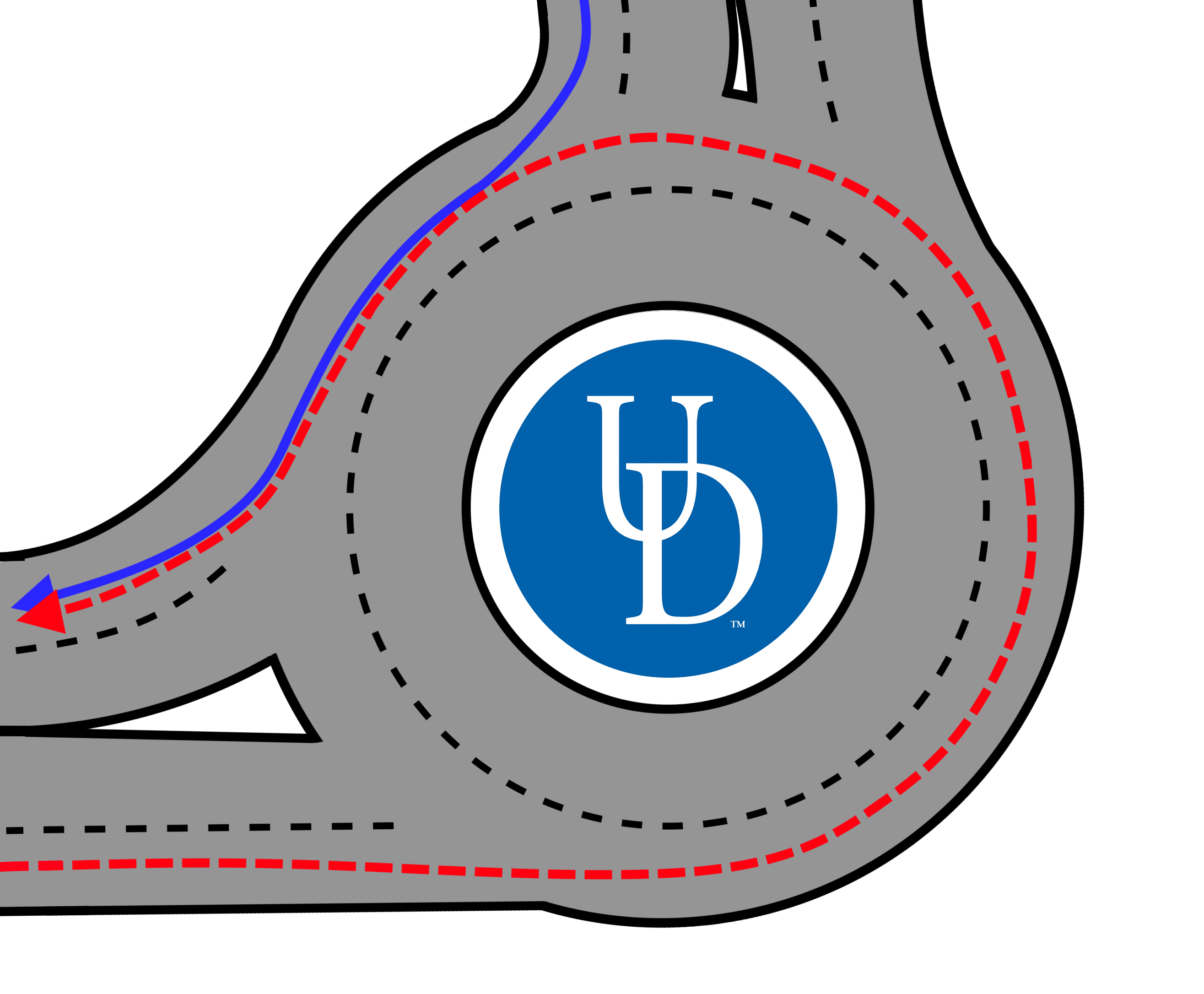
Figure 1: The routes taken by the northern (solid blue) and western (dashed red) groups through the roundabout.

III-A Reinforcement Learning Structure

We categorize two sets of RL experiments that are used and compared in this article. We will refer to them as: Gaussian single-agent: A single-agent policy trained with Gaussian noise injected into the state and action space. Adversarial multi-agent: A multi-agent policy trained wherein a second agent provides selective adversarial noise to the learning agent. We discuss the particulars of these two methods in Sections III-A4 and III-A5. In this article, we deploy seven RL-trained policies, one of which is single-agent with no noise, three of which are Gaussian single-agent and the other three of which are adversarial multi-agent. All experiments follow the same setup. Inflows of stochastic length emerge at the northern and western ends of the roundabout. The size of the northern group will range from $2$ to $5$ cars, while the size of the western group ranges from $2$ to $8$. The length of these inflows will remain static across each rollout, and are randomly selected from a uniform distribution at the beginning of each new rollout.

III-A1 Action Space

The actions are applied from a $2$-dimensional acceleration vector, in which the first element is used to control the AV leading the northern group, and the second is used to control the AV leading the western group. If the AV has left the experiment, that element of the action vector is discarded.

III-A2 State Space

The state space conveys the following information about the environment to the agent: the position, velocity, tailway, and headway of each AV and each vehicle in the roundabout, the distance from the roundabout entrances to the $6$ closest vehicles, the velocities of the $6$ closest vehicles to each roundabout entrance, the number of vehicles queued at each entrance, and the lengths of each inflow. All elements of the state space are normalized. The state space was designed with real-world implementation in mind and could contain any environmental factors that the simulation supports. As such, it is partially-observable to support modern sensing capabilities. All of these observations are reasonably selected and could be emulated in the physical world using sensing tools such as induction loops, camera sensing systems, and speedometers.

III-A3 Reward Function

The reward function used for all experiments minimizes delay and applies penalties for standstill velocities, near-standstill velocities, jerky driving, and speeding, i.e.,

$$r_{t}=2\cdot\frac{\max\left({v_{\text{max}}\sqrt{n}-\sqrt{\sum_{i=1}^{n}(v_{i,t}-v_{\text{max}})^{2}}},0\right)}{v_{\text{max}}\sqrt{n}}-p,$$ (3)

$$p=p_{s}+p_{p}+p_{j}+p_{v}.$$ (4)

where $n$ is the total number of vehicles, $p$ is the sum of four different penalty functions, $p_{s}$ is a penalty for vehicles traveling at zero velocity, designed to discourage standstill; $p_{p}$ penalizes vehicles traveling below $0.2m/s$, which discourages the algorithm from learning an RL policy which substitutes extremely low velocities to circumvent the zero-velocity penalty; $p_{j}$ discourages jerky driving by maintaining a dynamic queue containing the last $10$ actions and penalizing the variance of these actions; and $p_{v}$ penalizes speeding.

III-A4 Gaussian single-agent noise

Injecting noise directly to the state and action space has been shown to aid with transfer from simulation to real-world testbeds [21, 32]. In this method, which applies to three of the policies we deployed, each element of the state space was perturbed by a random number selected from a Gaussian distribution. Only two elements describing the length of the inflows approaching the merge were left unperturbed. Elements of the state space corresponding to positioning on the merge edge were perturbed from a Gaussian distribution with a standard deviation of $0.05$. For elements corresponding to absolute positioning, the standard deviation was 0.02. All other elements used a standard deviation of $0.1$. These values were selected to set reasonable bounds for the degree of perturbation in the real world. Each element of the action space was perturbed by a random number selected from a zero mean Gaussian distribution with $0.5$ standard deviation.

III-A5 Adversarial multi-agent noise

For the other $3$ policies, we use a form of adversarial training to yield a policy resistant to noise [33]. This is a form of multi-agent RL, in which two policies are learned. Adversarial training pits two agents against each other in a zero-sum game. The first is structurally the same as the agent which is trained in the previous $4$ policies. The second, adversarial agent has a reward function that is the negative of the first agent’s reward; in other words, it is incentivized by the first agent’s failure. The adversarial agent can attempt to lower the agent reward by perturbing elements of the action and state space of the first agent.

The adversarial agent’s action space is a 1-dimensional vector of length $22$, composed of perturbation values bound by $[-1,1]$. The first two elements of the adversarial action space are used to perturb the action space of the original agent’s action space. Adversarial action perturbations are scaled by $0.1$. Combining adversarial training with selective randomization, the adversarial agent has access to perturb a subset of the original agent’s state space. The remaining $20$ elements of the adversarial agent’s action space are used to perturb $20$ selective elements of the original agent’s state space. Both the adversarial action and state perturbations are scaled down by $0.1$. The selected elements that the adversary can perturb are the observed positions and velocities of both controlled AVs in the system and the observed distances of vehicles from the merge points.

IV Simulation Framework

IV-A Car Following Parameters

As introduced in Section  II-C, the human-driven vehicles in these simulations are controlled via IDM. Accelerations are provided to the vehicles via (1) and (2). Within these equations, $s_{0}$ is the minimum spacing or minimum desired net distance from the vehicle in front of it, $v_{0}$ is the desired velocity, $T$ is the desired time headway, $\delta$ is an acceleration exponent, $a$ is the maximum vehicle acceleration, and $b$ is the comfortable braking deceleration.

Human-driven vehicles in the system operate using SUMO’s built-in IDM controllers, which allows customization to the parameters described above. Standard values for these parameters as well as a detailed discussion on the experiments producing these values can be found in [26]. In these experiments, the parameters of the IDM controllers are defined to be $T=1~{}\text{s}$ , $a=1~{}\text{m}/\text{s}^{2}$ , $b=1.5~{}\text{m}/\text{s}^{2}$, $\delta=4$, $s_{0}=2~{}\text{m}$, $v_{0}=30~{}\text{m}/\text{s}$. A noise parameter $0.1$ was used to perturb the acceleration of the IDM vehicles.

Environment parameters in the simulation were set to match the physical constraints of the experimental testbed. These include: a maximum acceleration of $1~{}\text{m}/\text{s}^{2}$, a maximum deceleration of $-3~{}\text{m}/\text{s}^{2}$, and a maximum velocity of $8~{}\text{m}/\text{s}$. The timestep of the system is set to $1~{}\text{s}$.

IV-B Algorithm/Simulation Details

We ran experiments with a discount factor of $0.999$, a trust-region size of $0.01$, a batch size of $20000$, a horizon of $500$ seconds, and trained over $100$ iterations. The controller is a neural network, a Gaussian multi-layer perceptron with a tanh non-linearity, and hidden sizes of $(100,50,25)$. The choice of neural network non-linearities, size, and type were picked based on traffic controllers developed in [20]. The states are normalized so that they are between $0$ and $1$ by dividing each state by its maximum possible value. The agent actions are clipped to be between $-3$ and $1$. Both normalization and clipping occur after the noise is added to the system so that the bounds are properly respected. The following codebases are needed to reproduce the results of our work. Flow, SUMO and the version of RLlib used for the RL algorithms is available on GitHub.

IV-C Simulation Results

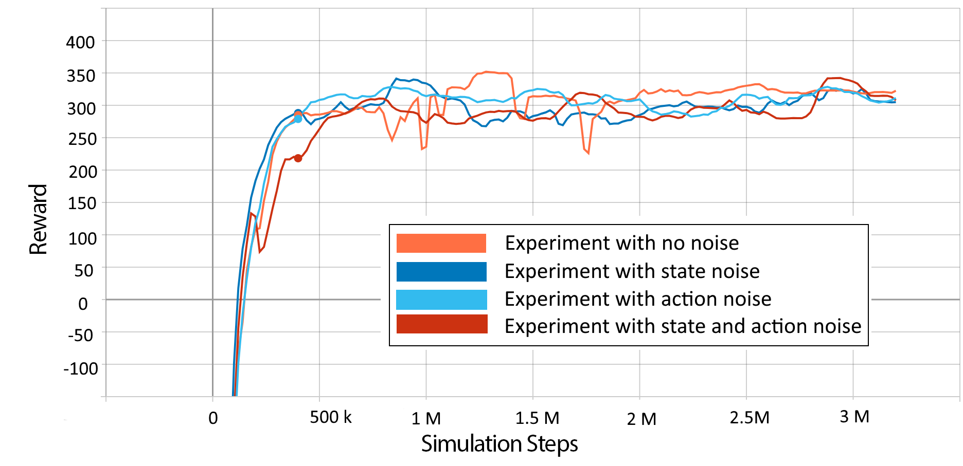
Figure 2: Convergence of the RL reward curves of the 3 Gaussian experiments and the noiseless policy.

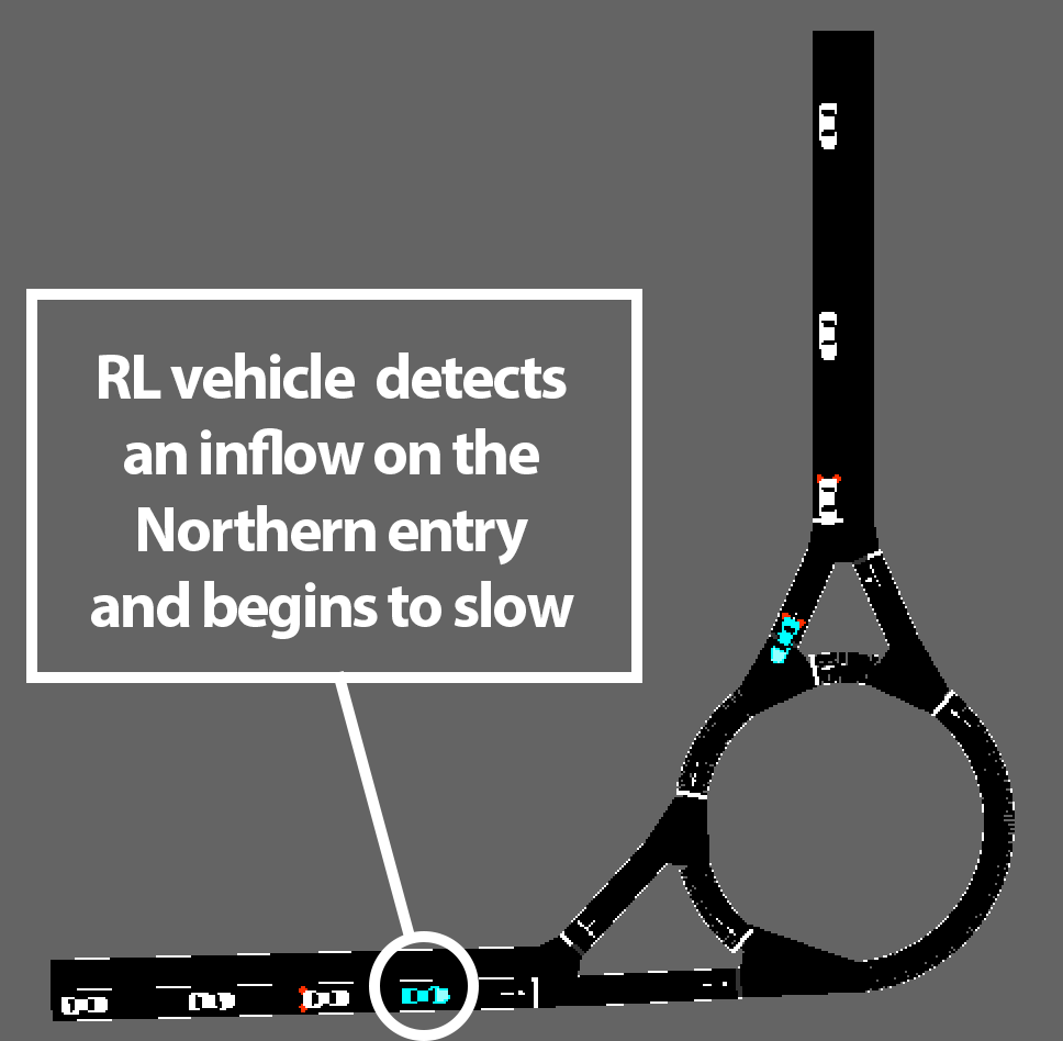
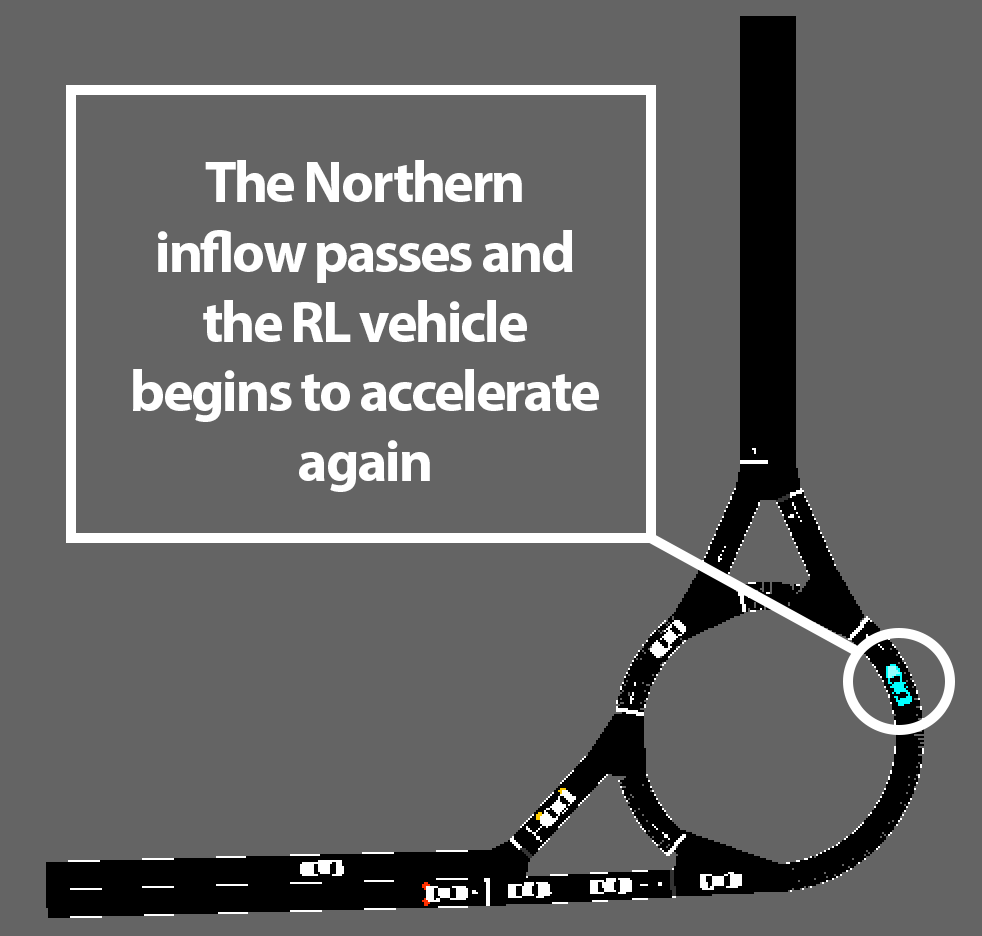
Figure 3: Two RL-controlled AVs trained with adversarial multi-agent noise demonstrate emergent ramp metering behavior.

The reward curves of the Gaussian single-agent experiments are displayed in Fig. 2. These include the curves of the $3$ experiments, which are trained with Gaussian noise injection, as well as one trained without any noise. In both the Gaussian single-agent and adversarial multi-agent experiments, the policy learns a classic form of traffic control: ramp-metering, in which one group of vehicles slows down to allow for another group of vehicles to pass. Despite the varying length of inflows from the two entries, policies consistently converge to demonstrate ramp-metering.

V Experimental Deployment

V-A The University of Delaware’s Scaled Smart City

University of Delaware’s Scaled Smart City (UDSSC) is a $1$:$25$ scale testbed designed to replicate real-world traffic scenarios and implement cutting-edge control technologies in a safe and scaled environment. UDSSC is a fully integrated smart city, which can be used to validate the efficiency of control and learning algorithms, including their performance on physical hardware. UDSSC utilizes high-end computers and a VICON motion capture system to simulate a variety of control strategies with as many as $35$ scaled CAVs. For further information on the capabilities and features of the UDSSC, see [34].

UDSSC utilizes a multi-level control architecture to precisely position each vehicle using position feedback from a VICON motion capture system. High-level routing and desired velocity calculation is handled by the mainframe computer, as well as locating the vehicle relative to each street on the map. This information is sent to each CAV which then calculates its desired steering and velocity actions based on a Stanley Controller [35, eq. (9)], and the velocity control for each non-RL vehicle is specified by the IDM controller (1).

To implement the RL policy in UDSSC, the weights of the network generated by Flow were exported into a data file. This file was accessed through a Python script on the mainframe, which uses a ROS service to map the current state of the experiment into a control action for each RL vehicle. During the experiment, the RL vehicles took commands from this script as opposed to the IDM controller.

To generate a disturbance on the roundabout system, a random delay for when each group was released was introduced. This delay was uniformly distributed between $0$ and $1$ seconds for the western group and between $0$ and $4$ seconds for the northern group during UDSSC experiments. The size of each vehicle group was randomly selected from a uniform distribution for each trial.

V-B Experimental Results

The data for each vehicle was collected through the VICON motion capture system and is presented in Table I. The position of each car was tracked for the duration of each experiment, and the velocity of each car was numerically derived with a first order finite difference method.

TABLE I: Experimental results for the baseline (no RL) case and each training method.

Training	Mean	Mean	Trials	% Time	Crashes
	Time (s)	Speed (m/s)		Saved
Baseline	23.6	0.23	47	-	0
Adversarial Multi-Agent
Action-State	22.1	0.24	29	+6.3	0
Action	22.1	0.23	23	+6.4	0
State	21.4	0.24	26	+9.6	10
Gaussian Single-Agent
Action-State	25.8	0.21	26	-9.2	0
State	23.0	0.23	18	+2.6	0
Action	23.1	0.22	37	+2.4	0
Noiseless	22.8	0.23	32	+3.5	0

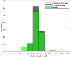
(a)

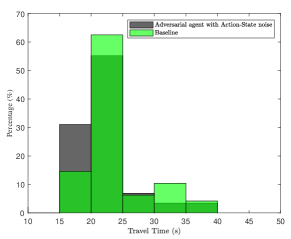
(b)

Figure 4: A relative frequency histogram for LABEL:sub@a the mean speed and LABEL:sub@b travel time of each vehicle for the baseline and adversarial multi-agent scenarios with noise injected in action and State.

For all trials, the RL vehicle exhibited the learned ramp metering behavior, where the western leader reduced its speed to avoid yielding by the northern group. The metering behavior was extreme for the Gaussian single-agent noise case, especially when noise was added to the action and state together. This excessive metering significantly reduced the average speed and increased travel delay, as seen in Table I. The adversarial multi-agent training significantly outperformed the Gaussian single-agent and tended to leave only a single vehicle yielding at the northern entrance. This strategy led to a travel time reduction for the northern group without a significant delay in western vehicles. The adversarial multi-agent case with noise injected only into the state accelerated especially fast and led to several catastrophic accidents between the two RL vehicles. Finally, for small numbers of vehicles, the adversarial multi-agent trained controllers appeared to exhibit an emergent zipper merging behavior.

Relative frequency histograms of average travel time and mean speed for the adversarial multi-agent case with noise injected into both action and state versus baseline scenarios are overlaid in Fig. 4. Over all trials, the adversarial case had a higher relative frequency of shorter travel time compared to the baseline scenario. Average travel time for $30\%$ of adversarial scenarios, lies in the range $[15\text{s},20\text{s}]$ comparing to $15\%$ for the baseline scenarios.

From Table I, we can see the average speed for baseline and the adversarial multi-agent with noise in action-state are nearly the same. However, in Fig. 4, we can see that approximately $8\%$ of trials in the baseline scenarios have an average speed between $0.1$ m/s and $0.15$ m/s. Furthermore, there are some trials that the average speed of the baseline scenario is between $0.35$ m/s and $0.4$ m/s. On the other hand, the average speed for the adversarial multi-agent with noise in action and state varies less, and near $65\%$ of trials have the average speed between $0.2$ m/s and $0.25$ m/s compared to $55\%$ in the baseline scenarios.

VI Conclusion

In this article, we developed a zero-shot transfer of an autonomous driving policy directly from simulation to the UDSSC testbed. Even under stochastic, real-world disturbances, the adversarial multi-agent policy improved system efficiency by reducing travel time and average speed for most vehicles.

As we continue to investigate approaches for policy transfer, some potential directions for future research include: multi-agent adversarial noise with multiple adversaries, tuning to determine which elements of the state space are most suitable for perturbations, tuning injected noise to maximize policy robustness, larger, more complex interactions, such as intersections, or merging at highway on-ramps, and longer tests involving corridors with multiple bottlenecks.

References

- [1] B. Schrank, B. Eisele, T. Lomax, and J. Bak, “2015 Urban Mobility Scorecard,” tech. rep., Texas A& M Transportation Institute, 2015.
- [2] L. Zhao and A. A. Malikopoulos, “Enhanced mobility with connectivity and automation: A review of shared autonomous vehicle systems,” IEEE Intelligent Transportation Systems Magazine, 2020 (forthcoming).
- [3] Z. Wadud, D. MacKenzie, and P. Leiby, “Help or hindrance? the travel, energy and carbon impacts of highly automated vehicles,” Transportation Research Part A: Policy and Practice, vol. 86, pp. 1–18, 2016.
- [4] J. Lee and B. Park, “Development and Evaluation of a Cooperative Vehicle Intersection Control Algorithm Under the Connected Vehicles Environment,” IEEE Transactions on Intelligent Transportation Systems, vol. 13, no. 1, pp. 81–90, 2012.
- [5] H. Rakha and R. K. Kamalanathsharma, “Eco-driving at signalized intersections using v2i communication,” in Intelligent Transportation Systems (ITSC), 2011 14th International IEEE Conference on, pp. 341–346, IEEE, 2011.
- [6] A. A. Malikopoulos, C. G. Cassandras, and Y. J. Zhang, “A decentralized energy-optimal control framework for connected automated vehicles at signal-free intersections,” Automatica, vol. 93, pp. 244 – 256, 2018.
- [7] A. A. Malikopoulos, S. Hong, B. B. Park, J. Lee, and S. Ryu, “Optimal control for speed harmonization of automated vehicles,” IEEE Transactions on Intelligent Transportation Systems, vol. 20, no. 7, pp. 2405–2417, 2018.
- [8] M. Athans, “A unified approach to the vehicle-merging problem,” Transportation Research, vol. 3, no. 1, pp. 123–133, 1969.
- [9] J. Rios-Torres and A. A. Malikopoulos, “Impact of partial penetrations of connected and automated vehicles on fuel consumption and traffic flow,” IEEE Transactions on Intelligent Vehicles, vol. 3, no. 4, pp. 453–462, 2018.
- [10] J. Rios-Torres and A. A. Malikopoulos, “A Survey on Coordination of Connected and Automated Vehicles at Intersections and Merging at Highway On-Ramps,” IEEE Transactions on Intelligent Transportation Systems, vol. 18, no. 5, pp. 1066–1077, 2017.
- [11] J. Guanetti, Y. Kim, and F. Borrelli, “Control of connected and automated vehicles: State of the art and future challenges,” Annual Reviews in Control, 2018.
- [12] Y. Wang, X. Li, and H. Yao, “Review of trajectory optimisation for connected automated vehicles,” IET Intelligent Transport Systems, 2018.
- [13] J. Guanetti, Y. Kim, and F. Borrelli, “Control of connected and automated vehicles: State of the art and future challenges,” Annual Reviews in Control, vol. 45, pp. 18–40, 2018.
- [14] S. Gu, E. Holly, T. Lillicrap, and S. Levine, “Deep reinforcement learning for robotic manipulation with asynchronous off-policy updates,” in Robotics and Automation (ICRA), 2017 IEEE International Conference on, pp. 3389–3396, IEEE, 2017.
- [15] D. Silver, J. Schrittwieser, K. Simonyan, I. Antonoglou, A. Huang, A. Guez, T. Hubert, L. Baker, M. Lai, A. Bolton, et al., “Mastering the game of go without human knowledge,” Nature, vol. 550, no. 7676, p. 354, 2017.
- [16] “Alphastar: Mastering the real-time strategy game starcraft ii,” Jan 2019.
- [17] R. E. Stern, S. Cui, M. L. Delle Monache, R. Bhadani, M. Bunting, M. Churchill, N. Hamilton, H. Pohlmann, F. Wu, B. Piccoli, et al., “Dissipation of stop-and-go waves via control of autonomous vehicles: Field experiments,” Transportation Research Part C: Emerging Technologies, vol. 89, pp. 205–221, 2018.
- [18] Y. Sugiyama, M. Fukui, M. Kikuchi, K. Hasebe, A. Nakayama, K. Nishinari, S.-i. Tadaki, and S. Yukawa, “Traffic jams without bottlenecks—experimental evidence for the physical mechanism of the formation of a jam,” New journal of physics, vol. 10, no. 3, p. 033001, 2008.
- [19] C. Wu, A. Kreidieh, E. Vinitsky, and A. M. Bayen, “Emergent behaviors in mixed-autonomy traffic,” in Conference on Robot Learning, pp. 398–407, 2017.
- [20] E. Vinitsky, A. Kreidieh, L. Le Flem, N. Kheterpal, K. Jang, F. Wu, R. Liaw, E. Liang, and A. M. Bayen, “Benchmarks for reinforcement learning in mixed-autonomy traffic,” in Conference on Robot Learning, pp. 399–409, IEEE, 2018.
- [21] K. Jang, E. Vinitsky, B. Chalaki, B. Remer, L. Beaver, A. Malikopoulos, and A. Bayen, “Simulation to scaled city: zero-shot policy transfer for traffic control via autonomous vehicles,” in 2019 International Conference on Cyber-Physical Systems, (Montreal, CA), 2019.
- [22] F. Belletti, D. Haziza, G. Gomes, and A. M. Bayen, “Expert level control of ramp metering based on multi-task deep reinforcement learning,” IEEE Transactions on Intelligent Transportation Systems, 2017.
- [23] R. Bellman, “A markovian decision process,” Journal of Mathematics and Mechanics, pp. 679–684, 1957.
- [24] J. Schulman, F. Wolski, P. Dhariwal, A. Radford, and O. Klimov, “Proximal policy optimization algorithms,” arXiv preprint arXiv:1707.06347, 2017.
- [25] J. Schulman, S. Levine, P. Abbeel, M. Jordan, and P. Moritz, “Trust region policy optimization,” in International Conference on Machine Learning, pp. 1889–1897, 2015.
- [26] M. Treiber, A. Hennecke, and D. Helbing, “Congested traffic states in empirical observations and microscopic simulations,” Physical review E, vol. 62, no. 2, p. 1805, 2000.
- [27] C. Wu, A. Kreidieh, K. Parvate, E. Vinitsky, and A. M. Bayen, “Flow: Architecture and benchmarking for reinforcement learning in traffic control,” arXiv preprint arXiv:1710.05465, 2017.
- [28] E. Liang, R. Liaw, R. Nishihara, P. Moritz, R. Fox, J. Gonzalez, K. Goldberg, and I. Stoica, “Ray rllib: A composable and scalable reinforcement learning library,” arXiv preprint arXiv:1712.09381, 2017.
- [29] Y. Duan, X. Chen, R. Houthooft, J. Schulman, and P. Abbeel, “Benchmarking deep reinforcement learning for continuous control,” in International Conference on Machine Learning, pp. 1329–1338, 2016.
- [30] D. Krajzewicz, J. Erdmann, M. Behrisch, and L. Bieker, “Recent development and applications of SUMO - Simulation of Urban MObility,” International Journal On Advances in Systems and Measurements, vol. 5, pp. 128–138, December 2012.
- [31] G. Brockman, V. Cheung, L. Pettersson, J. Schneider, J. Schulman, J. Tang, and W. Zaremba, “Openai gym,” arXiv preprint arXiv:1606.01540, 2016.
- [32] J. Tobin, R. Fong, A. Ray, J. Schneider, W. Zaremba, and P. Abbeel, “Domain randomization for transferring deep neural networks from simulation to the real world,” in Intelligent Robots and Systems (IROS), 2017 IEEE/RSJ International Conference on, pp. 23–30, IEEE, 2017.
- [33] L. Pinto, J. Davidson, R. Sukthankar, and A. Gupta, “Robust adversarial reinforcement learning,” in Proceedings of the 34th International Conference on Machine Learning-Volume 70, pp. 2817–2826, JMLR. org, 2017.
- [34] L. E. Beaver, B. Chalaki, A. M. Mahbub, L. Zhao, R. Zayas, and A. A. Malikopoulos, “Demonstration of a Time-Efficient Mobility System Using a Scaled Smart City,” Vehicle System Dynamics, vol. 58, no. 5, pp. 787–804, 2020.
- [35] G. M. Hoffmann, C. J. Tomlin, M. Montemerlo, and S. Thrun, “Autonomous automobile trajectory tracking for off-road driving: Controller design, experimental validation and racing,” in 2007 American Control Conference, pp. 2296–2301, July 2007.