Imaging Higher Dimensional Black Objects
Abstract
We develop a systematic ray-tracing method which can be used to explore a wide class of higher-dimensional multi-center black objects through the shape of their shadows. As a proof of principle, we test our method by imaging black holes and black rings in five dimensions. Two-dimensional slices of the three-dimensional shadows of those five-dimensional black objects not only show new phenomena, such as the first image of a toroidal horizon, but also offer a new viewpoint on black holes and binary systems in four dimensions.
Keywords:
Black holes, Black Holes in String Theory1 Introduction
It is well known that the black hole uniqueness theorems in General Relativity (GR) are specific to vacuum GR in four dimensions. In more than four dimensions or when gravity is coupled to matter fields, a plethora of new black hole solutions comes into play. In more than four spacetime dimensions, black objects exist with distinct horizon topologies but with the same masses and spins Emparan:2008eg. Coupling GR to matter fields gives rise to black hole solutions with scalar, fermionic or vector hair; configurations of matter fields outside the horizon111See e.g. Herdeiro:2015aa; Volkov:2016aa for recent reviews.. In this context, one even has compact objects without horizons from self-gravitating bosonic configurations known as boson stars. Other extensions of GR, involving higher derivatives, quantum effects, etc, similarly lead to modifications of the unique GR horizon. This richness of compact objects in extensions of GR has spawned vast fields of study, ranging from exploring the intrinsic theoretical properties of those solutions to fleshing out all the many possibilities for testing GR with recent and future observations of black holes in nature.
String theory combines all of the above richness. Its extra dimensions and the many matter fields arising in compactifications mean that the wide variety of gravitational black hole like solutions is already evident at the classical level. The low-energy limit of string theory, supergravity, has a vast set of solutions that are absent in 3+1 vacuum GR. To leading order in the string length expansion, supergravity theories are two-derivative Lagrangians with couplings to matter fields in up to eleven spacetime dimensions. The solution space contains the three types of solutions mentioned above: non-spherical horizon topologies, hairy black holes, and horizonless solutions. The causal structure and other spacetime properties of the vast number of solutions has remained largely unexplored. The reason is simply the complexity of most of those solutions. Even the earliest known black ring in pure GR in 4+1 dimensions Emparan:2001wn has a non-integrable geodesic problem Grunau:2012ai. Many more of the solutions with and without horizons have a high degree of asymmetry with at best one (timelike or null) Killing vector, but in general no other isometries.
With this paper, we aim to start a systematic numeric exploration of the many black hole like solutions descending from string theory, by investigating their null geodesic structure and using this to image the compact objects. We develop and present a backwards ray tracing code and a visualization scheme adapted to axisymmetric but otherwise arbitrary asymptotically flat, supersymmetric solutions of five-dimensional ungauged supergravity coupled to vector multiplets, described in Gutowski:2004yv; Elvang:2004ds; Gauntlett:2004qy; Bena:2004de and reviewed in Bena:2007kg.
We choose this class of five-dimensional supersymmetric solutions for two reasons. First, five is the lowest number of dimensions allowing both new horizon topologies and smooth horizonless solutions. Second, due to supersymmetry the solution space is linear in the sense that one can add sources freely and thus identify solutions with an arbitrary number of centers. Whereas specific solutions of pure GR in higher dimensions need to be run case by case, our code enables the imaging of many solutions in a fast manner: The restriction to axial symmetry, or more properly one timelike and two rotational Killing vectors in 5D, is enough to reduce the numerical integration time to the order of hours on a normal laptop, for an image of pixels.
To demonstrate our method, we produce ray-traced images of Breckenridge-Meyers-Peet-Vafa (BMPV) black holes Breckenridge:1996is and supersymetric black rings of Emparan, Elvang, Mateos and Reall Elvang:2004rt. To the best of our knowledge, these are the first ray-traced images of higher-dimensional objects222Analytic result on the black hole shadow exist for Myers-Perry black holes Papnoi:2014aaa. and the first images of black rings altogether. As a verification of our method, we compare the numerically generated BMPV shadows with analytically computed shadows cast by BMPV black holes and find perfect agreement. Two-dimensional slices of these ray-traced images exhibit all known features of rotating black holes in four dimensions, including the characteristic shape of near-extremal images due to frame dragging.
Our images of black rings reveal new features. Depending on which two-dimensional slicing one considers, the images can serve different purposes. While the black ring horizon has topology , one possible 2D slicing has the topology of two disconnected two-spheres. Imaging this reveals the same key features known for binary systems in four dimensions, such as disconnected shadows with characteristic ‘eyebrows’ Nitta:2011in; Yumoto:2012kz; Bohn:2014xxa; Patil:2016oav; Shipley:2016omi; Wang:2017qhh; Cunha:2018gql; Cunha:2018cof. This opens up a new analytic avenue for exploring four-dimensional black hole binaries. Other 2D slicings of black ring shadows show the first examples of shadows of toroidal horizons333A toroidal shadow of a horizon with spherical topology has been observed earlier, see Cunha:2016bjh., which can appear as concentric annuli in the two-dimensional projection. We do not compare to analytic results for black rings as those are only available for a restricted set of geodesics Grunau:2012ri.
The rest of this paper is organized as follows. In section 2, we give the details of our visualization scheme and integration method. In section 3, we discuss the BMPV black hole metric, its ray-traced images and compare to analytic results. In section 4 we discuss our images of supersymmetric black rings from different viewing angles and explain the salient features. We end with a summary and outlook on the many future imaging paths forward in section 5. The appendices contain the following supplementary material: Appendix A has a technical review of the full class of multi-center solutions to explain our conventions. We provide a derivation of the geodesic equations for axisymmetric multi-center solutions in appendix LABEL:sec:geodesics, and we end with the calculation of the geodesic equations and the shadow contour for BMPV black holes in appendix LABEL:sec:BMPV_exact.
2 Integration and Visualization Procedure
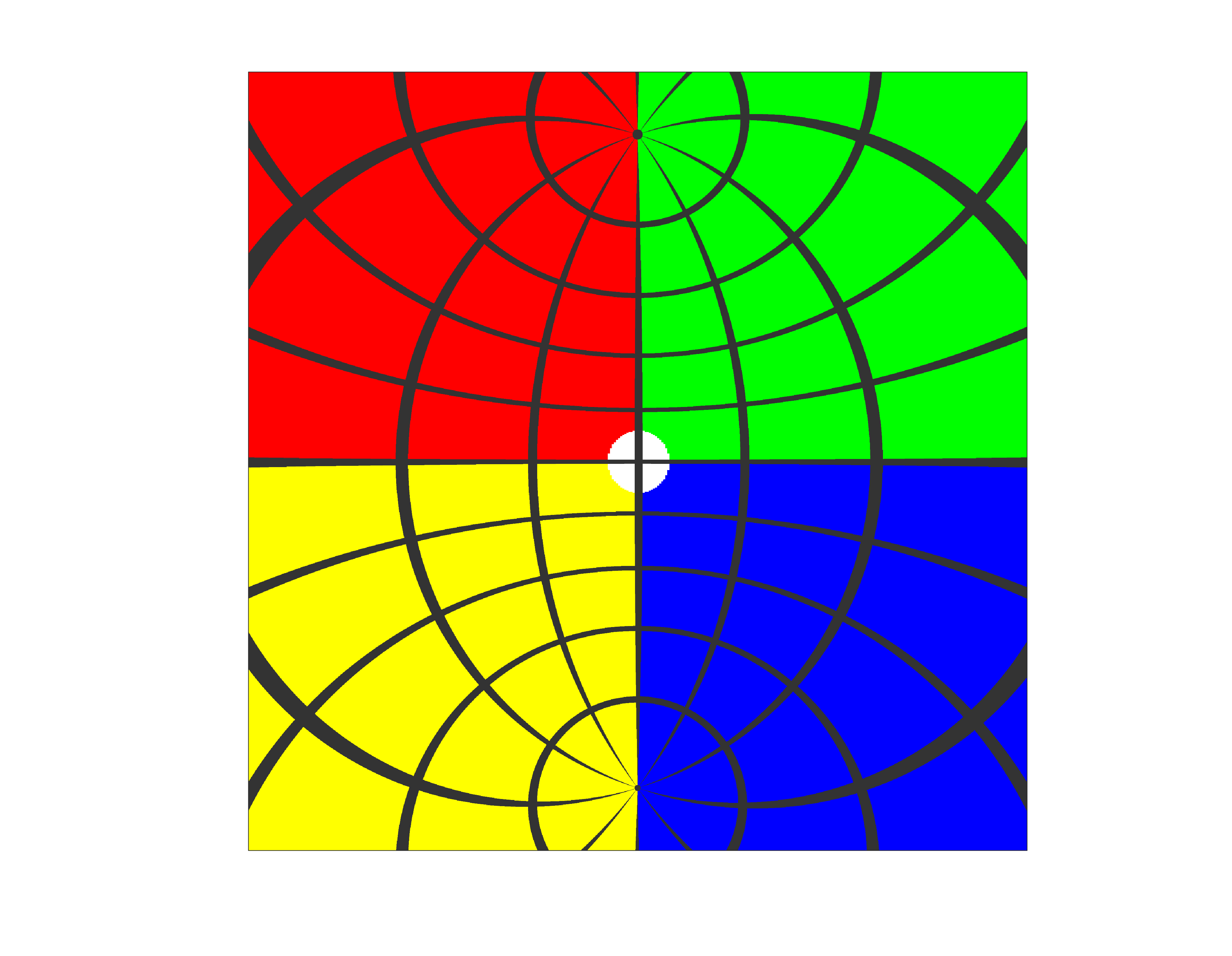
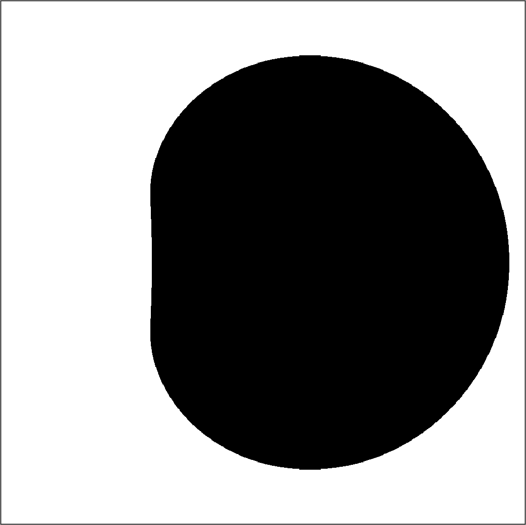
To create an image we use an extension of the setup discussed in Bohn:2014xxa; Cunha:2015yba; Cunha:2018acu. Readers who want to get to the physics can skip this section and just keep in mind that following the procedure with no central object gives the reference image in figure 1.
The goal is to assign a color to each pixel on a 2D slice of the three-dimensional screen constructed in the local sky of an asymptotic observer. We do this in three steps. First we associate a geodesic to each direction in the observer’s local sky (section 2.1). Next we follow this geodesic numerically until it either escapes or falls behind a horizon (section 2.2). And finally we associate a color to this geodesic depending on where it ended up (section 2.3).
2.1 The Local Sky
The first step is to associate a geodesic to each direction in the local sky of our observer in four-dimensional space. To bring this into practice, we will relate a set of local Cartesian coordinates for the asymptotic observer , to an appropriate global Cartesian coordinate system , see figure 2. We then express the asymptotic direction (a vector in the observer’s frame) to null geodesics in the global spacetime coordinates.
The local set of Cartesian axes has its origin at the position of the observer. Without loss of generality, we can choose this to be
| (1) |
with the inclination and the Cartesian distance from the origin. A direction in which the observer is looking is then represented by a unit vector in this local Cartesian frame. Before we can continue we need to fix these local Cartesian axes in some way. We can begin by putting the axis in the radial direction towards the origin of the spacetime. Due to our choice of position this lies in the plane of the global Cartesian coordinates. We can pick the axis to be in the plane perpendicular to the axis, and we orient it such that it points in the positive direction. We take the –axis and –axis to be aligned with the –axis and –axis respectively. This construction is illustrated in figure 2.
Next we represent a vector in this local frame in the spacetime coordinates. If we start with a vector in the local frame with components we can calculate what its components are in the global Cartesian frame with some simple geometry:
{IEEEeqnarray}rCl
v_x_1 &= -v_xsini - v_zcosi
v_x_2 = -v_y
v_x_3 = -v_xcosi + v_zsini
v_x_4 = -v_w.
At this point we have a map from a local vector to a null geodesic in the spacetime. To get a flat image we map a set of rectilinear coordinates to a local vector. To do this we use a Mercator like projection similar to the one used in Bohn:2014xxa; Cunha:2015yba; Cunha:2018acu:
{IEEEeqnarray}rCl
v_x &= k_0
v_y = k_0(2a-1)tan(αy2) = k_0 ¯v_y
v_z = k_0(2b-1)tan(αz2) = k_0 ¯v_z
v_w = k_0(2c-1)tan(αw2) = k_0 ¯v_w,
the , and effectively represent different camera apertures and the is a normalization constant which we will use to fix the energy of the geodesic. We can now form an image made up of discrete voxels by discretizing the three coordinates . This is useful to get an idea of the shape of the shadow which a full 5D observer would see. But this is not a very convenient way to study the lensing effects since different areas will be hidden behind and inside each other. To study the lensing effects it is better to take 2D slices of the full 3D space and then discretize this 2D subspace to get an image made out of pixels.
The multi-center solutions of our interest are naturally written in Gibbons-Hawking coordinates . To apply the above steps, we bring the asymptotic form of the metric into standard Cartesian coordinates on flat space by the coordinate redefinition:
{IEEEeqnarray}rCl
x_1 &= 2rcos(ϕ+ ψ2)cos(θ2),
x_2 = 2rsin(ϕ+ ψ2)cos(θ2),
x_3 = 2rcos(ψ2)sin(θ2),
x_4 = 2rsin(ψ2)sin(θ2).
The coordinate distance and inclination are then:
| (2) |
In appendix LABEL:sec:geodesics we show how we to set up the initial value problem at fixed energy in Gibbons-Hawking coordinates. The result is that we solve the system of equations given by (LABEL:eq:geod) starting from the initial conditions (LABEL:eq:init).
2.2 Numerical Integration
We now have set up an initial value problem (IVP) for each triplet in camera space. To solve the IVP we use the following procedure:
-
1.
We integrate the IVP by using for example the RKDP method as implemented in the ODE45 function of the MATLAB ODE suite (in the future a more specialized integrator can be used).
-
2.
To handle coordinate singularities we use event location to stop the integration when we get close and decrease the tolerance of the integrator. We estimate when we have moved far enough away from the singularity and check if we have indeed done so when we reach that point. If we have, we increase the tolerance back to the original value and continue, otherwise we estimate again and keep the tolerance.
-
3.
We end the integration when we reach one of two possible exit conditions. The first is if the geodesic is back at the same radial coordinate at which it started, this signifies that it has escaped to infinity. The second condition is if we are within a chosen small Cartesian distance from a horizon, in this case we say that the geodesic has fallen behind the horizon.
-
4.
To estimate the integration error we calculate the RMS of along each geodesic (see appendix LABEL:sec:geodesics). If this is larger than a predetermined tolerance we reject this geodesic and restart the integration with more stringent tolerances.
Those four steps provide a map from the camera coordinates to either the horizon or to some position far away from the object.
2.3 Color Coding
As a third and final step, we associate the final position of each geodesic to a color. All the geodesics which fell behind the horizon are marked black. The geodesics which escaped from the central object are colored according to the given reference image. In principle this image is three-dimensional. We will always restrict to a 2D subspace first and apply the colour coding afterwards as follows. First we convert the 4D final positions of the escaped geodesics to Cartesian coordinates. Next we take the 3D subspace containing the radial direction from our observer and the two directions corresponding to the chosen hypersurface. In this 3D subspace we can go to standard spherical coordinates and map the polar angle to the vertical direction of the image and the azimuthal direction to the horizontal direction of the image. This gives us an RGB value for each escaped geodesic. Using this visualization an observer would see figure 1 if there is no central object in the way.
3 Supersymmetric Black Holes
Perhaps the simplest non-trivial metric in the multi-center class we describe is the Breckenridge-Myers-Peet-Vafa (BMPV) black hole Breckenridge:1996is. It describes the 5D version of the extremal Reissner-Nordstrom metric.
3.1 Metric
We work with the form of the metric adapted to the multi-center extension described in appendix A:
| (3) |
with the functions
| (4) |
Four-dimensional flat space is written as a particular Gibbons-Hawking fibration Hawking:1976jb; Gibbons:1979zt over with radial coordinate : {IEEEeqnarray}rCl ds^2_4 (R^4)&= r (dψ+ (1+cosθ) dϕ)^2+ r^-1 (dr^2 + r^2 (dθ^2 +sin^2 θdϕ^2)). The relation to Cartesian coordinates is given by (2).
3.2 Physical Properties
The BMPV black hole has an electric charge and two angular momenta. We label those as and in standard Euclidean coordinates . Supersymmetry imposes the extremality constraint on the mass and equality of the angular momenta:
| (5) |
with the 5D Newton constant. We will chose units such that . The fact that the solution has rotation might seem surprising from GR intuition, since in 3+1 dimensions, black holes can have only one independent rotation that is required to vanish by invariance under supersymmetry. In 4+1 dimensions however, black holes can have two independent rotations in two orthogonal planes; supersymmetry requires only one combination of them to vanish.
The horizon has the topology of , a three-sphere, with horizon area . As for the Kerr metric, too large values of the angular momenta can lead to pathologies. Positive horizon area requires . For larger angular momenta, the solution becomes ‘over-spinning’ and has naked Closed Timelike Curves. Those can be resolved invoking higher-dimensional effects Gibbons:1999uv; Herdeiro:2000ap; Herdeiro:2002ft; Drukker:2004zm. We choose to focus on imaging BMPV black holes with only in this paper.
3.3 Images
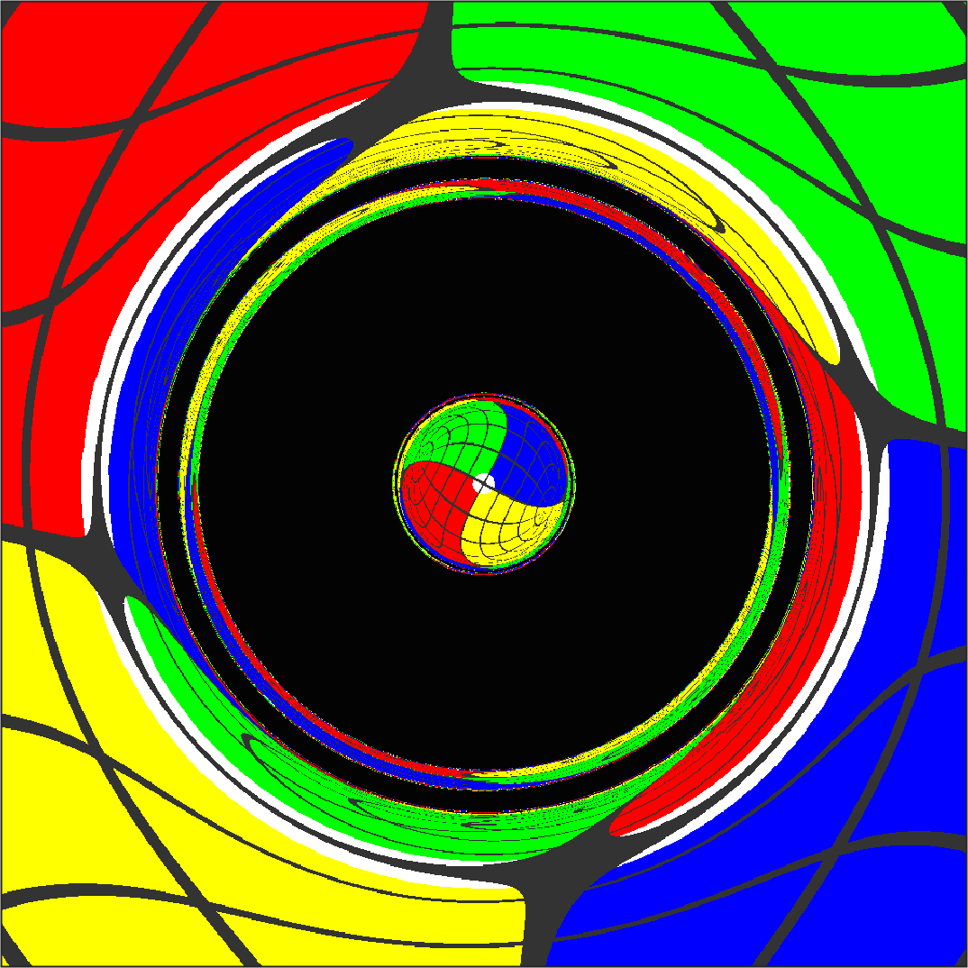
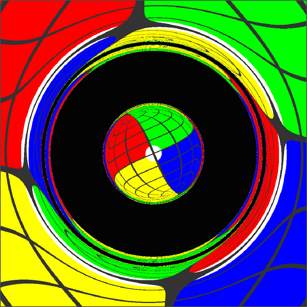
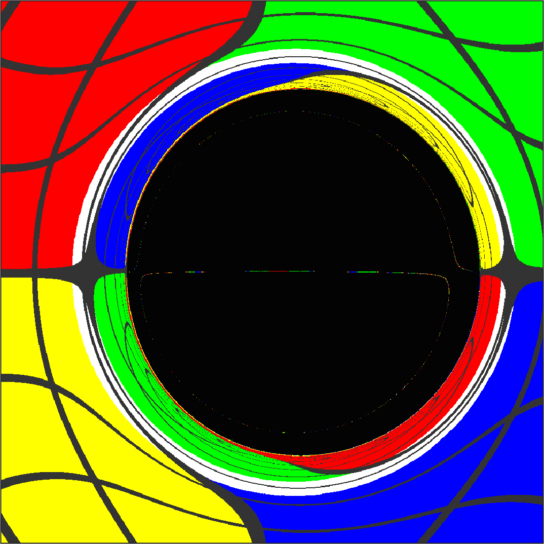
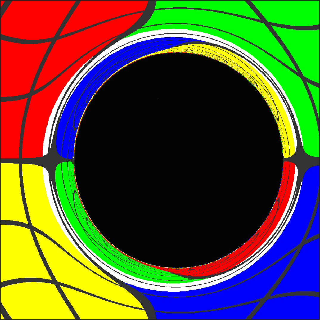
For imaging purposes, we will always suppress one dimension by fixing one of the four Cartesian spatial coordinates to zero. To clarify the basic physics picture, we choose inclination angle and suppress one direction. By symmetries of the black hole metric, there are two interesting choices for the remaining 3 axes. Either there is non-zero angular momentum in the horizontal plane containing line of sight (“edge on”), or we see non-zero angular momentum in the plane perpendicular to the line of sight (“face on”). We present the images for 3 different values of the rotation parameter in figure 3.


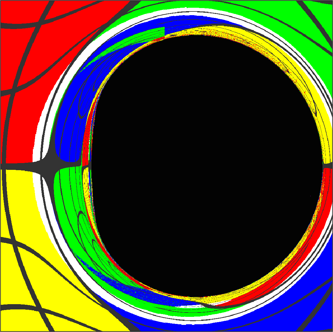


The images of the shadow show very similar behaviour as known from the rotating Kerr solution. Even though the horizon itself of the BMPV black hole is a non-rotating null hypersurface Gauntlett:1998fz, we do not see this effect in the shadow, since it images the light ring rather than the event horizon. As the angular momentum is increased, the shadow center shifts to the right, while the left side develops a flat side—the characteristic D-shape image known for rotating Kerr. This is due to the frame-dragging (on the left side of the image, rotation is oriented out of page). The edge-on view, with rotation perpendicular to line of sight, only shows the frame dragging in the image outside the round shadow.
We end this section with a comparison to analytic results. Since the geodesic problem in the BMPV background is Liouville integrable Gibbons:1999uv, one can separate the geodesic and wave equations Herdeiro:2000ap; Diemer:2013fza. We can then can obtain the equation for the edge of the black hole shadow following the same method as for the Kerr black hole. In appendix LABEL:sec:BMPV_exact we perform those calculations for the three-charge generalization of the BMPV black hole and discuss the equation for the shadow edge in terms of the impact parameters and inclination angle.
We found agreement between numerical and analytic results for the shadow edge up to numerical precision for our chosen resolution. For angular momentum close to the extremal value the numerical integration near the shadow edge is more error-prone due to the inner and outer horizon nearly coinciding. We still find agreement within our image resolution. For reference, we plot the analytic shadow in the bottom row of figure 3.
4 Supersymmetric Black Rings
Our second example is the supersymmetric black ring Elvang:2004rt; Bena:2004de.
4.1 Metric
We write the metric again in the form
| (6) |
with the coordinates (4). The black ring has two centers (two poles in harmonic functions): one located at the origin of , the other we put at the positive -axis at a distance . This is reflected in the form of and :
{IEEEeqnarray}rCl
Z &= 1 + Q-q24 Σ + q2r4 Σ2,
k = [(q3r28 Σ3-3 q r (q2-Q)16 Σ2)(1+cos(θ))+3 q (4 r+R2)8 Σ-3 q2] dϕ
+ [q3r28 Σ3-3 q r (q2-Q)16 Σ2+3 q (4 r+R2)16 Σ-3 q4] dψ,
with the coordinate distance of the ring location to the origin.
4.2 Physical Properties
Again this solution has an electric charge , but unlike the black hole it has two independent angular momenta. The origin of this freedom is the presence of a dipole charge , related to non-trivial magnetic fields:
| (7) |
Again we will put . The black ring has non-spherical horizon topology: the horizon has the topology of , a higher-dimensional torus with cross-section. The horizon area of the ring is the product of the length, with radius , and the area, which has radius :
| (8) |
As for the black hole, the requirement of positive horizon area puts a bound on the angular momenta. However, this is an insufficient condition for physical regularity. Absence of CTC’s requires also that . In addition the ring radius parameter should be positive. We plot the region of allowed ring solutions in the ( plane in figure 4. We choose to normalize the angular momenta by an appropriate power of the charge . This is not a mere fixing of scale, but is a judicious choice that makes use of the invariance of the spectrum of solutions of 5D supergravity coupled to vector multiplets under the rescaling:
| (9) |
which map solutions to solutions. Hence the two-dimensional diagram truly represents all solutions in this three-parameter class of black rings.

Depending on the ratio of ring circumference by cross-sectional area, set by , we can distinguish two distinct types of black rings. When that ratio is close to its minimal value , we have a ‘thick ring’, shaped like a higher-dimensional donut with a relatively small hole in the middle. For we have a ‘thin ring’. One can check that thick rings have values of angular momenta that are nearly equal (close to the black hole vlaues), while the thinnest rings have . We will see below that indeed thin rings generate quite a different image than black holes.
As a final remark, we note that although classically the charges take on a continuous range of values, charge quantization in string theory requires and to take on discrete values.
4.3 Images
Unlike for the black hole, different slicings are now giving physically distinct two-dimensional images for a given viewing angle. Upon fixing one Cartesian direction, the two-dimensional projection of the horizon area will be either two disconnected ’s, or a two-dimensional torus with topology. For each projections we show two different viewing angles that we dub “face-on” and “edge-on”, see table 1 for an overview. We will make most plots in the order of the table, see figure 5. Unless stated otherwise, we take the camera at coordinate distance , with defined as in (2).
| Coord. | Topology | Inclination | along LOS | along screen |
|---|---|---|---|---|
| 2 ’s | (Face on) | |||
| 2 ’s | (Edge on) | |||
| (Face on) | ||||
| (Edge on) |
|
|
|
|
|
|---|---|---|---|
|
 |
 |
 |

|
 |
 |
 |
4.3.1 Disconnected Two-sphere Topology
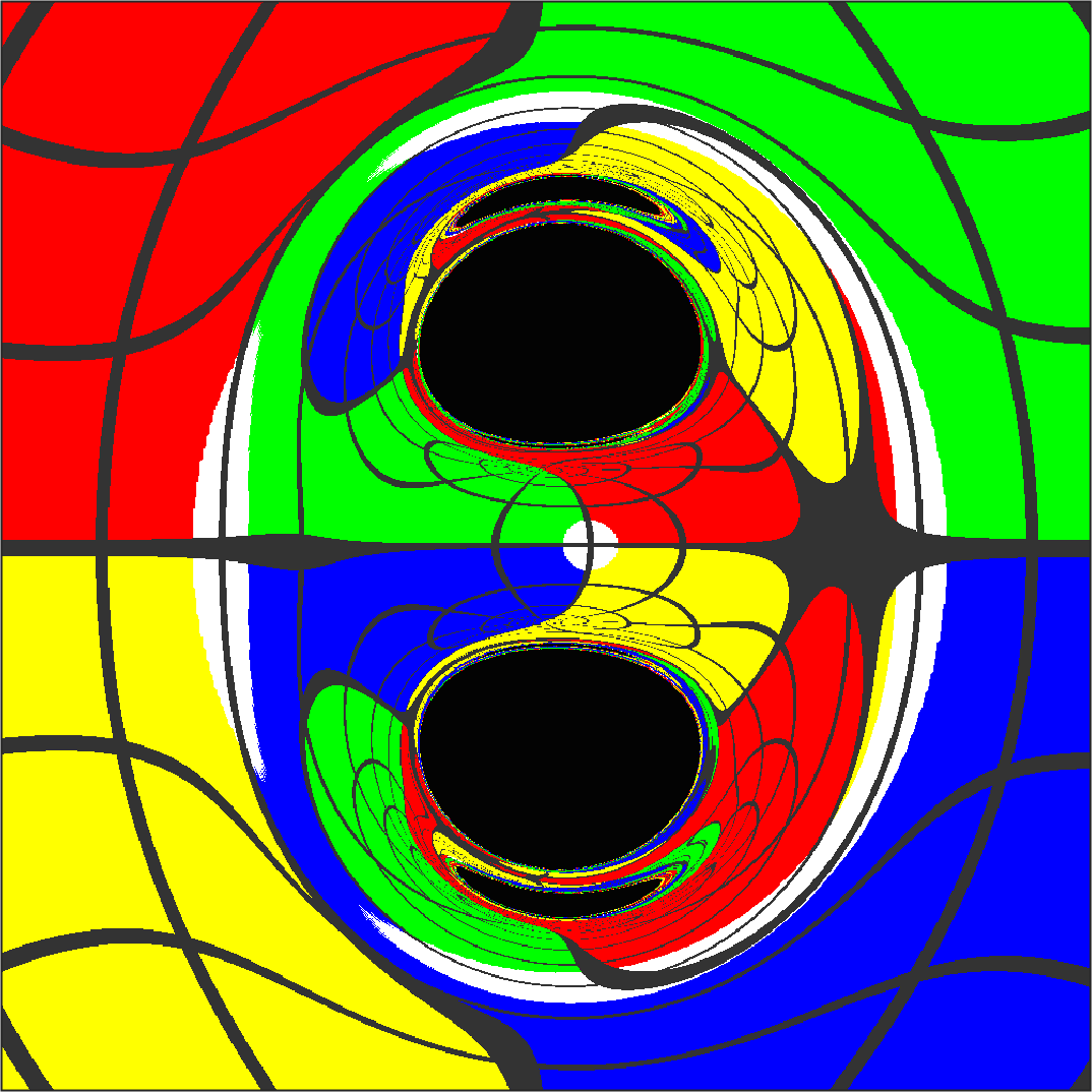
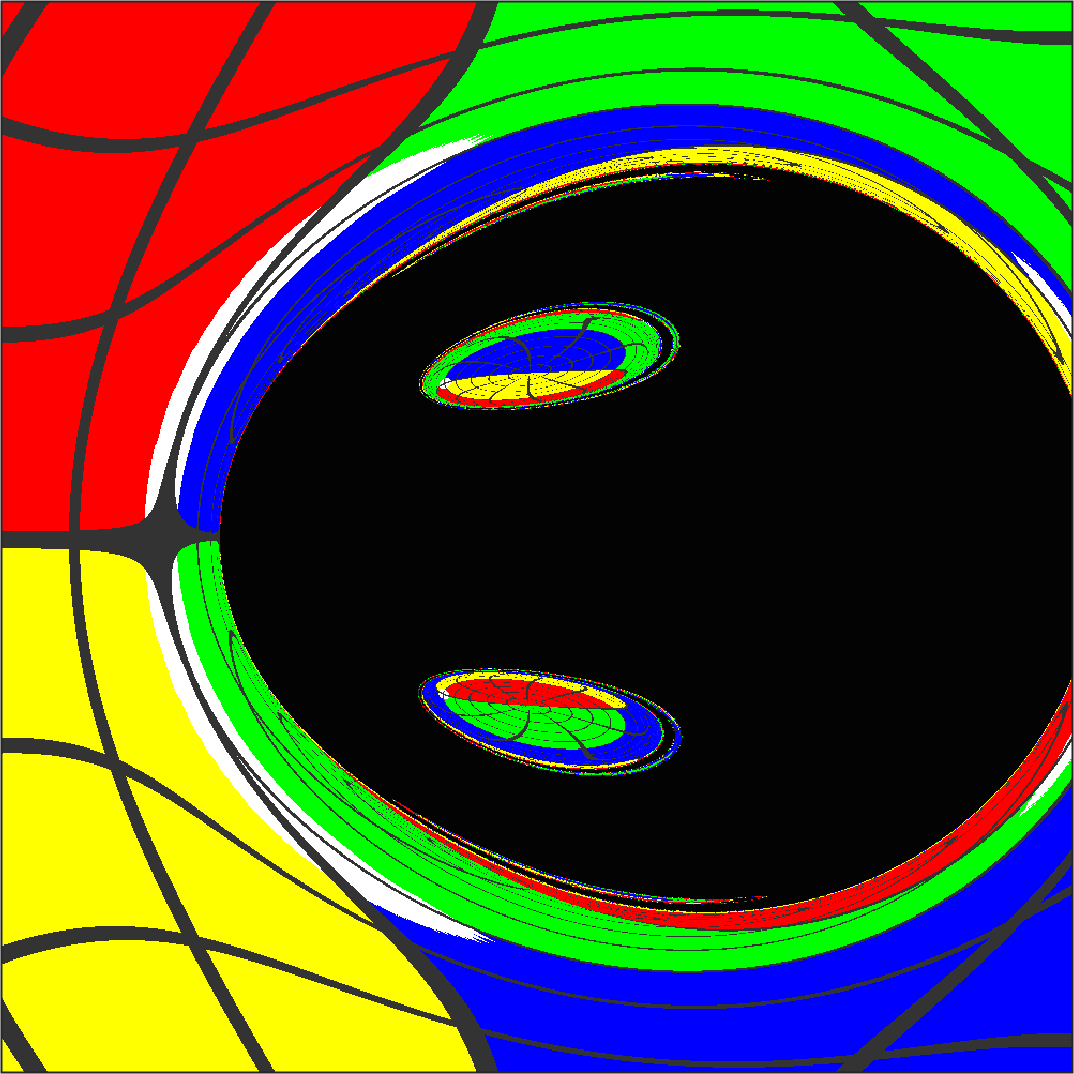
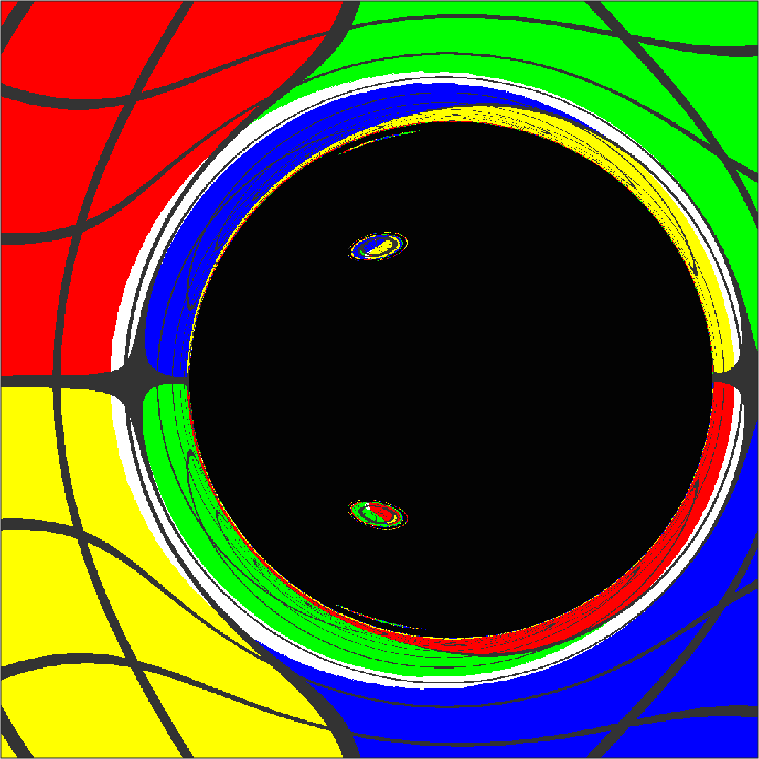
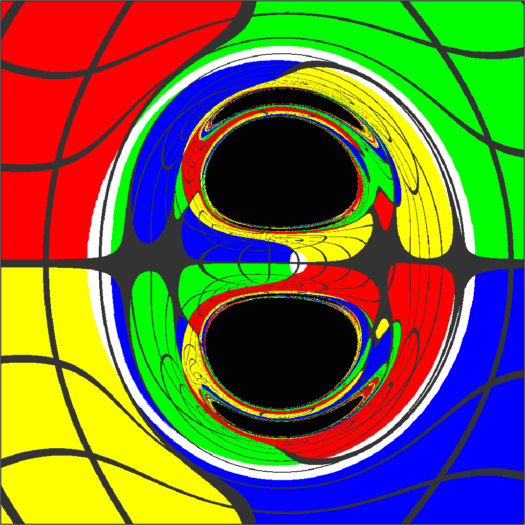
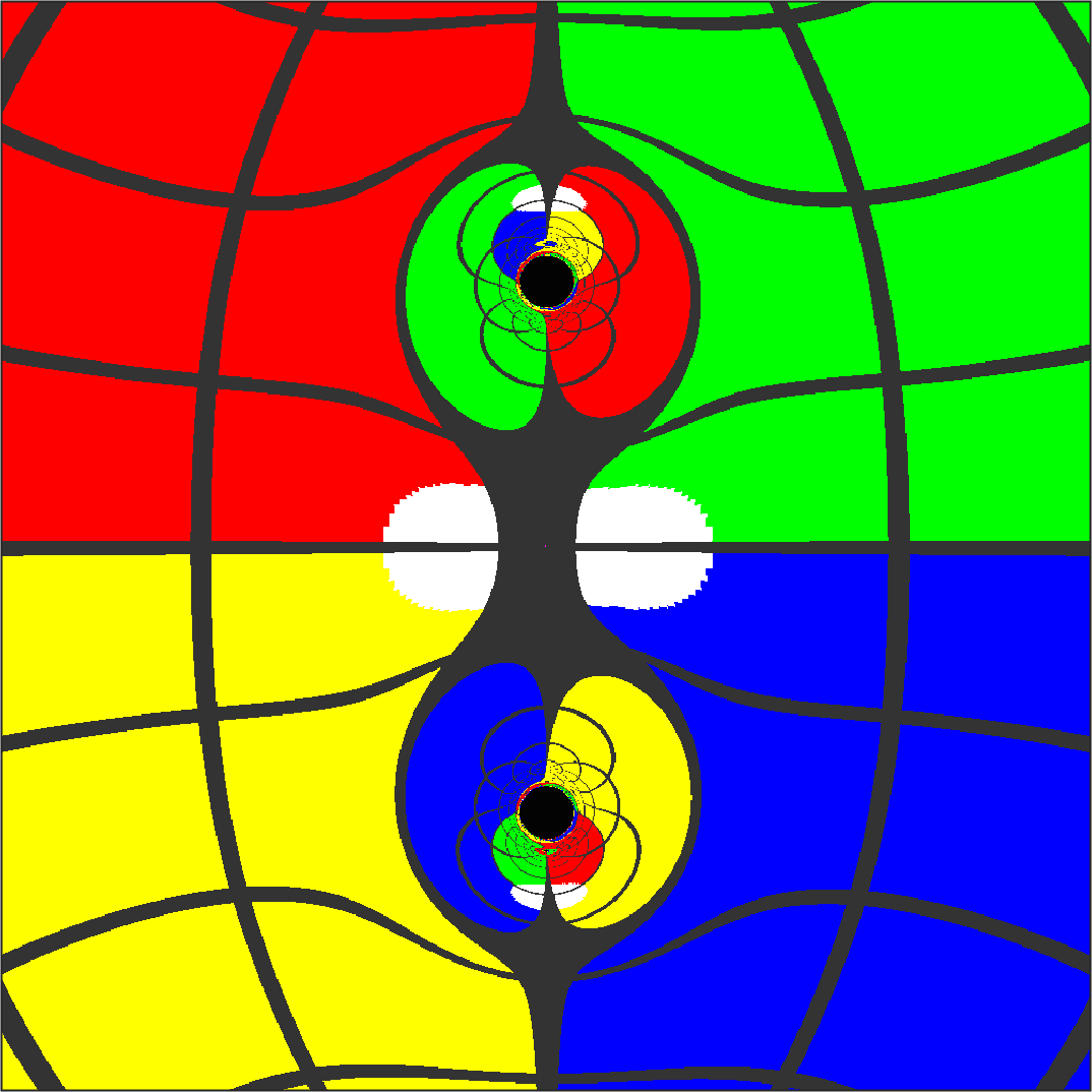
First we fix to obtain the 2D slicing of the horizon with disconnected two-spheres (left 2 columns of figure 5). As one might expect, the images show a striking resemblance to earlier visualizations of binary black holes Bohn:2014xxa and we recover the main features. When viewed face on (inclination ), we clearly see the shape of the two disconnected parts of the horizon. At the outer edges, we also recognize the distinct ‘eyebrows’, the flattened image of one part of the horizon from lensing around the other disconnected part Nitta:2011in; Yumoto:2012kz. When imaging this slicing edge on (inclination ), the ’s and the camera align. The shadow of the farthest appears as a ring around the central shadow of the closer object. Such an image is similar to the visualization of an in-spiraling binary system shown in Bohn:2014xxa.
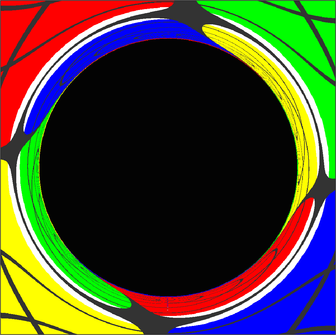
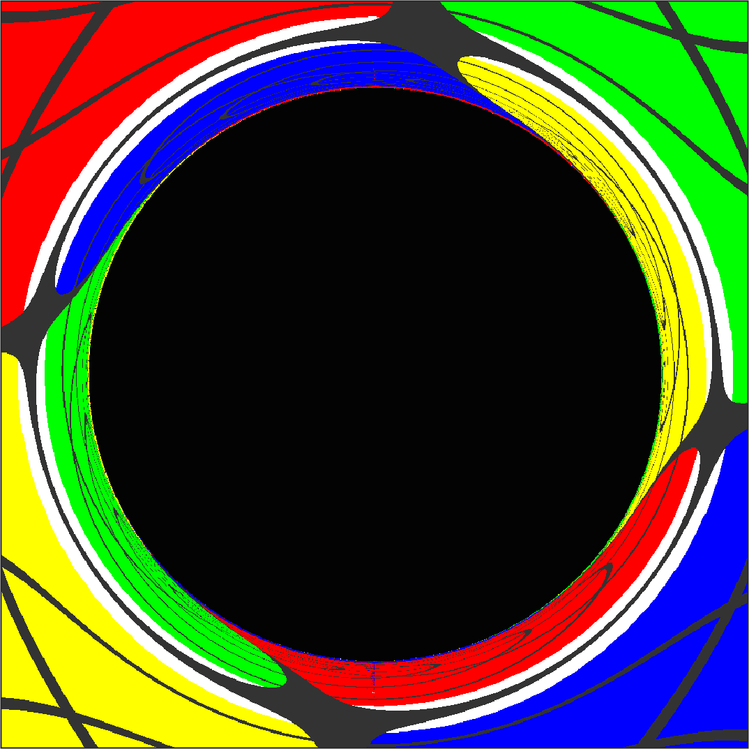
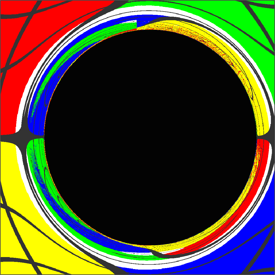
To investigate the appearance of chaotic effects due to lack of integrability, we zoomed in on one of the images, see figure 6. Binary black hole shadows are known to exhibit fractal structure Bohn:2014xxa; Shipley:2016omi and we confirm similar behaviour for black ring images. The black ring shadow shows a repeated structure of multiple eyebrows or concentric annuli, see figure 6. Although a more detailed study is outside the scope of this work, we think it would be a worthwhile to investigate this further in terms of distinct loci in spacetime and Lyapunov exponents according the lines of Grover:2017mhm.
We leave a more detailed comparison to known examples of two-center black holes to future work. For the supersymmetric rings we discuss in this paper, such a comparison would be most natural with extremal charged four-dimensional solutions, such as the two-center Papapetrou-Majumdar solution discussed in Yumoto:2012kz. The extension to uncharged black rings would be interesting as well.
4.3.2 Toroidal Topology
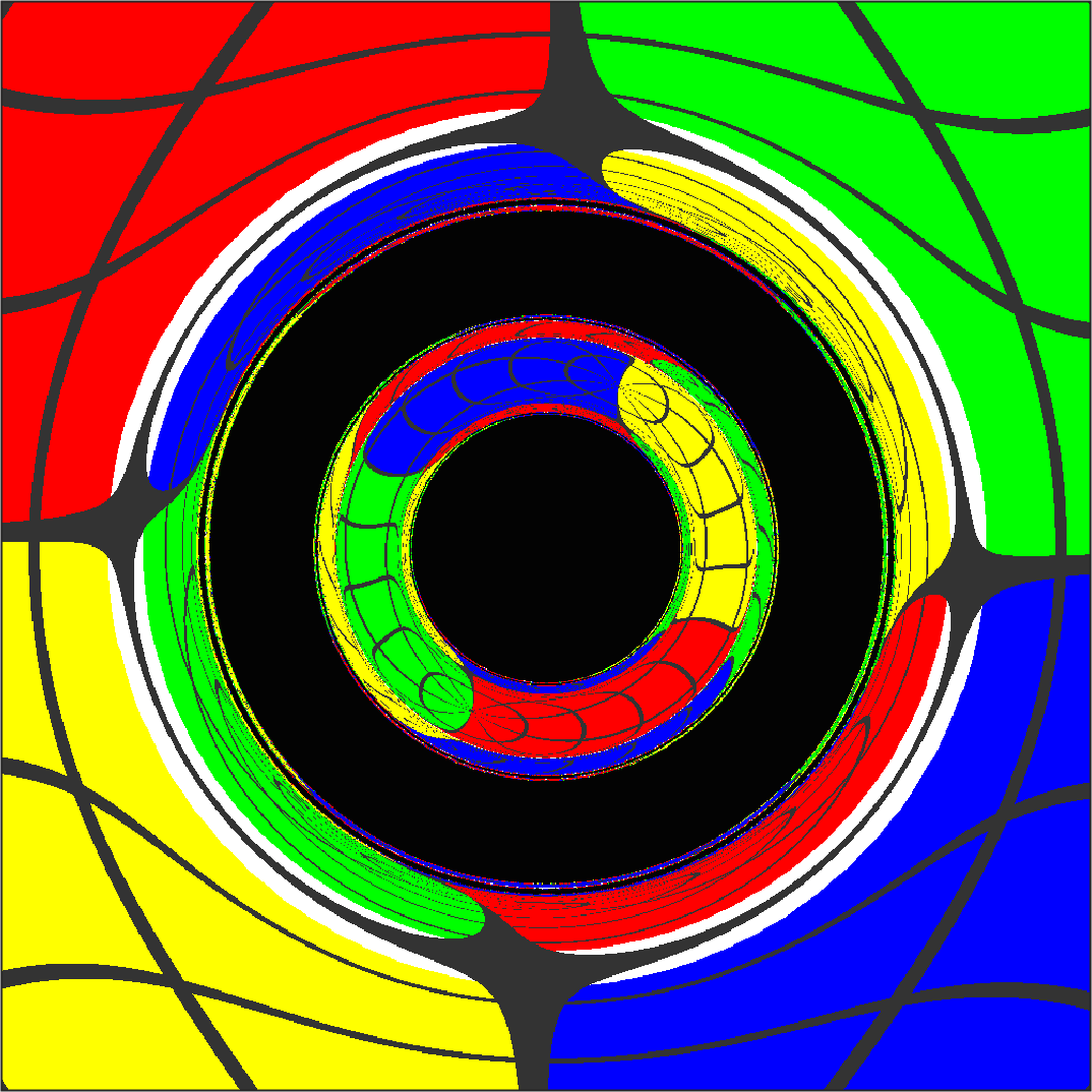
Next we fix . The 2D slice of the black ring horizon has the topology of , a two-dimensional torus. This is the first example of an image of a toroidal black shadow and its effects on the surrounding spacetime.
The two inclinations we choose show a number of new effects. When viewed face on (third column of figure 5), one can clearly distinguish two concentric black annuli: a central annulus with a black halo around it. Increasing precision reveals again a fractal-like looking structure of ever thinner concentric annuli as one moves away from the center of the image (figure 6). The innermost ring indicates geodesics hitting the ring directly, the secondary ring those geodesics that have one turning point and so on. The thickness of the inner ring depends on the ring parameters: for large values of , the ring radius greatly exceeds the radius of the cross-section and we naturally observe thinner rings with thinner annuli as a consequence.
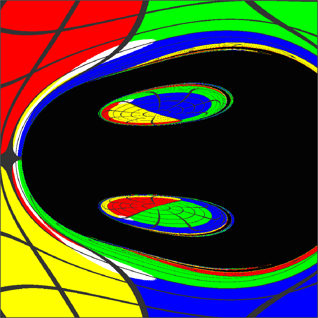
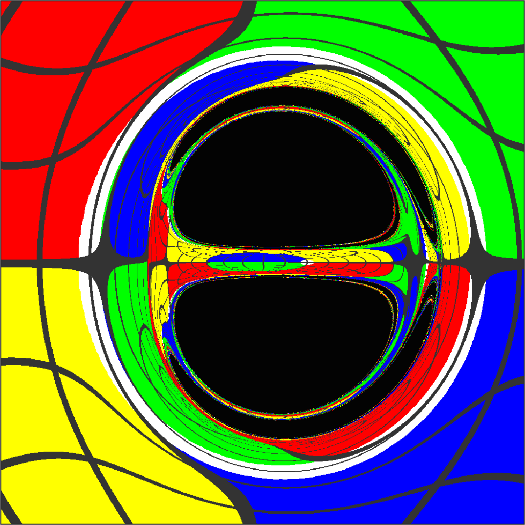
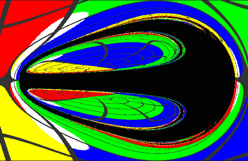
When viewed edge on (fourth column of 5), the image becomes most interesting. The shadow has three main features: an elongated shape, two holes, and a clear left-right asymmetry not of the D-shape kind known from earlier visualizations of rotating black objects:
-
•
The elongated shape reveals the shape of the ring. For larger values of , the ring becomes thinner and the image becomes more elongated.
-
•
The holes in the image arise from geodesics shooting through the ring from either above or below and escaping through infinity. By symmetry of the problem, the holes are symmetrically placed with respect to the horizontal axis and the holes intersect the vertical axis, as geodesics going through the ring and the origin of our coordinate system are always mapped to the vertical. We clearly distinguish two large holes near the horizontal axis and long thin holes near the shadow edge, with repeated shadow structure inside the holes (figure 6)444For completeness we note that in Fig 4a in Wang:2018aa a shadow of a Manko-Novikov solution is reported displaying two holes..
-
•
Both the holes and the shape of the shadow have a left-right asymmetry. For generic values of angular momenta, the shadow edges left and right are smoothly curved, with a smaller radius of curvature on the left part of the figure. The asymmetry itself is caused by the rotation along the ring plane (, along line of sight). The left-hand side of the image shows a part of the ring that is rotating towards the camera, which causes a contraction effect in the lensing, while the opposite is true for the right-hand side. The same effect happens for the holes. The angular momentum is only indirectly visible in the image: for fixed values of the , it influences the size of the ring and the shape of the shadow.
All three qualitative features are related to the topology and affected by the ratio of the two angular momenta as we discuss now.
4.3.3 Effects of Angular Momentum
We explore the phase space of allowed angular momenta for the black rings and compare to black holes with the same value of one of the two angular momenta. Recall that the is along the ring horizon , while is orthogonal. figure 5 shows two different solutions with constant , figure 7 shows three different solutions with constant .

When (left column in figure 7), black ring parameters are close the the black hole and unsurprisingly the image is almost indistinguishable from a black hole’s. In general, however, images of black rings differ quite a lot from the black hole image, and there is a lot of variation in size of the black ring compared to the black hole.
Having either one angular momentum along the line of sight, gives the clearest distinction of the black hole image, as it reveals either the disconnected or the elongated shape of the shadow, see figure 7. The bottom row in that figure shows an extremal spinning black ring, with maximal for given . The effect of rotation on the surrounding spacetime is visible in all images, but the effect on the shadow is as announced only visible when the angular momentum along the line of sight, that is, for the viewing angles of figure 7. The edge on view of the disconnected slicing (bottom left) does not shows the typical D-like shape in the individual shadows of the disconnected parts of the images, but we can see this effect still on the image outside the shadow, which shows resemblance to the extremal black hole image of figure 3. The edge-on view of the toroidal slice (bottom right) is interesting: the shadow acquires the typical D-like shape and shift off-center towards the right, as known for near-extremal Kerr. But still we see the holes characteristic to black ring solutions.
Finally we want to point out that extremal rings with larger ratios of the angular momenta resemble much less the black hole image, see figure 8. Such rings are very thin and their shadows remain elongated; the flattening of the shadow is present only at the very tip of the shadow.
5 Outlook
We have developed the numerical tools to explore multi-center black hole like solutions of string theory with null geodesics. As an application, we discussed images and shadows of supersymmetric black holes and black rings in five dimensions and we also showed how they give insight in four-dimensional physics. In this respect it is worth noting that the visualization of black rings in higher dimensions offers a novel and complementary view on binary systems in four dimensions. This may prove important since the imaging of binaries in dimensions has some technical limitations arising from the fact that one is mostly restricted to working with numerical solutions Bohn:2014xxa or solutions with conical singularities, such as the double Schwarzschild solution and double-Kerr solutions Cunha:2018gql; Cunha:2018cof. By contrast black rings are analytically known and non-singular. In this context it would be very interesting to adapt the quasi-static procedure of Cunha:2018cof and consider images of rotating black rings. We leave this to future work.
There are two further directions in which our calculations should be extended. First, with our ray-tracing and visualization technique in place, it can be immediately applied to more intricate black hole like solutions. We are currently working on imaging solutions with more than two centers in the wide class of five-dimensional multi-center solutions, such as multi-black holes, multi-rings, and horizon-less microstate geometries Hertog:inprep1. Ultimately, we deem it important to extend the method developed here to more generic spacetimes not restricted by supersymmetry.
Second we want to emphasize that 2D images using backwards ray-tracing are merely scratching the surface. There is a much broader set of analytic and numerical tools at our disposal to explore and study the spacetime structure in the neighbourhood of black objects. A very useful one, that can be obtained with similar integration methods, is the geodesic deviation near compact objects. As was noted in Tyukov:2017uig; Bena:2018mpb geodesic probes can reach extremely high tidal forces long before they reach the region where the geometry differs significantly from the corresponding black hole. We aim to use our code to check this explicitly for five-dimensional multi-center solutions. Other important extensions include using massive probes and the study of the effect of an environment around compact objects.
More generally speaking, studies along these lines (see also e.g. Giddings:2016btb) work towards bridging the gap between observations and string theory or quantum gravity. Imaging the shadow of resolvable supermassive black holes using upcoming results of the Event Horizon Telescope, but also the details of the ringdown encoded in gravitational wave signals of compact binaries, are largely determined by the nature of the light ring, the unstable photon orbit outside the black hole. Understanding the geodesic structure near and inside the light ring of alternative compact objects is thus key to flesh out any possible deviations from the GR paradigm; imaging objects constitutes an important step in that direction.
Acknowledgments
We thank Fabio Bacchini, Vitor Cardoso, Pedro Cunha, Roberto Emparan, Carlos Herdeiro, Stefanos Katmadas, Sera Markoff, Marina Martinez, Ben Niehoff, Bart Ripperda and Erik Verlinde for discussions; Fabio and Bart Ripperda also for input from a related collaboration and Perdo Cunha and Carlos Herdeiro for useful feedback on the manuscript. The authors are partially supported by the National Science Foundation of Belgium (FWO) grant G.001.12, the European Research Council grant no. ERC-2013-CoG 616732 HoloQosmos, the KU Leuven C1 grant ZKD1118 C16/16/005, the FWO Odysseus grant G0H9318N and the COST actions CA16104 GWVerse and MP1210 The String Theory Universe.
Appendix A Multi-center Solutions in 5D
In this section we give the larger class of metrics we study in one fixed notation, as different conventions have been used throughout the literature. We mostly follow Bena:2007kg.
We focus on supersymmetric, stationary, asymptotically flat solutions of 5D supergravity couple to an arbitrary number of vector multiplets with a timelike Killing vector. This class of solutions is written as a fibration of time over a four-dimensional space space Gauntlett:2002nw; Gauntlett:2003fk; Gutowski:2004yv
| (10) |
Supersymmetry requires the four-dimensional space to be hyperkähler. We restrict to the large subset of metrics for which the four-dimensional base space is a Gibbons-Hawking space. Those multi-center solutions were derived in five dimensions in Bena:2004de; Gauntlett:2004qy; Elvang:2004ds and reviewed in Bena:2007kg. The generic solution after reduction over the Gibbons-Hawking fibre originally given in Denef:2000nb; Bates:2003vx. For concreteness, we present the code and the solutions in the ‘STU model’ that arises in compactification of eleven-dimensional M-theory on (2 vector multiplets).
In section A.1 we only present the solution of the metric, not of the gauge fields nor the scalar fields, as those are not needed for our purposes. In section LABEL:ssec:explicit we write out the metric for an axisymmetric but otherwise arbitrary solution in the class. We recall how the black hole and black ring metrics we use are recovered in section LABEL:ssec:BH_BR.
A.1 Multi-center Solutions
The family of metrics of three–charge solutions with a Gibbons–Hawking base space is determined by eight harmonic functions on flat , with centers:
{IEEEeqnarray}rClCrCl
V &= v_0 + ∑_i=1^N viri K^I = k_0^I + ∑_i=1^N kIiri
L_I = l_0,I + ∑_i=1^N ℓI,iri M = m_0 + ∑_i=1^N miri,
where , are the locations of the centers which carry the harmonic charges and is an index that runs over the gauge fields (2 from the vector multiplets, one from the graviphoton). Those harmonic functions enter the metric (10) through intermediary functions , and one-forms :
{IEEEeqnarray}rCl
Z = (Z_1 Z_2 Z_3)^1/3 , k = μ(dψ+ A ) + ω , ds_4^2 = V^-1(dψ+A)^2 + V ds_3^2,
with the relations
{IEEEeqnarray}rCl
Z_I &= L_I + 12—ϵ_IJK —KJKKV,
μ= K1K2K3V2 + KILI2 V + M,
⋆_3 dA = dV,
⋆_3 dω= V dM - M dV
+ 12 (K^I dL_I - L_I dK^I). \IEEEeqnarraynumspace
Note that we allow the four-dimensional Gibbons-Hawking metric to be ‘ambipolar’, that is: it can flip signature from to between regions, by allowing to switch sign at the same location. The boundary region is known as an ‘evanescent ergosurface’ Bena:2007kg; Gibbons:2013tqa.
We get flat 5D asymptotics by setting , and . Then the ADM mass and electric charges are
{IEEEeqnarray}rCl
M &= π4G5(Q_1 + Q_2 + Q_3),
Q_I = 4∑_i=1^N(ℓ_I,i + 12—ϵ_IJK —k^J_ik^K_i).
The angular momenta can be obtained from a Komar integral, see for instance Emparan:2008eg for the normalization we use. We only give the full expression angular momenta below for axisymmetric solutions.
Generically these metrics will have CTC’s, a necessary requirement to avoid these are the bubble equations: {IEEEeqnarray}rCl m_0v_j + ∑