The $Z$ Penguin in Generic Extensions of the Standard Model

Abstract

Precision flavour observables play an important role in the interpretation of results at the LHC in terms of models of new physics. We present the result for the one-loop $Z$ penguin in generic extensions of the standard model which exhibit exact perturbative unitarity. We use Slavnov-Taylor identities to study the implications of unitarity on the renormalisation of the $Z$ penguin, and derive a manifestly finite result that depends on a reduced set of physical couplings.

1 Introduction

It is well known that precision flavour observables put strong constraints on models of new physics. While these models typically predict new particles which might be found by LHC experiments or at future colliders, first hints could show up as anomalies in precision flavour observables. Their examination could then lead to clues towards the nature of new physics. It is therefore of interest to calculate these observables in a generic extension of the standard model (SM).

We consider an arbitrary number of additional heavy degrees of freedom: gauge bosons, fermions and scalars. Perturbative unitarity imposes important constraints on such generic extensions. The required cancellation of unbounded high-energy growth of scattering amplitudes leads to specific relations among the coupling constants that are common to all models. These relations allow us to understand and perform the renormalisation of the observables in a general way. The feasibility of this approach is expected on general grounds since the equations implied by perturbative unitarity uniquely reflect the spontaneously broken gauge structure [1, 2, 3] and thus may as well be derived by means of Slavnov-Taylor identities (STI). Here we advocate the practical implementation of those simple relations in the calculation and renormalisation of generic loop amplitudes. This goes beyond the typical application of perturbative unitarity in which one derives upper bounds on yet unobserved mass spectra [4, 5, 6] and combinations of masses and/or couplings [7, 8, 9, 10, 11].

As an example we study the flavour-changing transition between two SM quarks $d_{j}$ and $d_{i}$ of different generations, induced by a heavy neutral gauge boson at one-loop for vanishing external momenta. An example is the FCNC $s\to d$ transition with the emission of a virtual $Z$ boson, the so-called $Z$ penguin. It contributes, in combination with flavor-changing box diagrams, to processes like the rare $K\to\pi\nu\bar{\nu}$ decays. Just like the SM, many models of new physics generate this transition first at the one-loop level, since their neutral SM-fermion currents are flavour-conserving. In this article we discuss the renormalisation of the general one-loop result for this process, assuming the absence of tree-level contributions to the $d_{j}\to d_{i}$ transition. Then we provide manifestly finite results for the special case of charged internal particles. It is then straightforward to obtain the $Z$ penguin in any given model by just inserting the specific couplings into our generic result. Due to sum rules derived from the STI, only a reduced set of couplings needs to be specified in practice. We illustrate this procedure in detail for several examples.

Our method has several interesting applications. It provides explicit and manifestly finite results for a very general class of extensions of the SM. The strategy is not restricted to flavour observables, but might also be applicable, for instance, to collider and dark-matter phenomenology.

This paper is organised as follows. After a definition of the generic Lagrangian in Sec. 2, we present in Sec. 4 the general analytic result which in many models is as yet unknown, and elaborate on its renormalisation. In Sec. 5 we explicitly perform the renormalisation of our result for the case of charged heavy particles. As an illustration, we (re-)derive the $Z$ penguin in various renormalisable models, to wit, the SM, the two-Higgs-doublet model, an extension of the SM with vector-like quarks, and the minimal supersymmetric SM (MSSM). In the appendices we give the results for the box diagrams in our notation and provide the definitions and explicit expressions of the requisite loop functions. Moreover, we provide the full list of Slavnov-Taylor identities for four-point couplings.

2 The generic Lagrangian

In this work we consider an extension of the SM by an arbitrary number of heavy scalar, fermion, and vector fields (in this context, “heavy” means that the particle masses are of the order of the electroweak scale or larger). As our starting point we define the parts of the generic Lagrangian which are relevant to the calculation of box and penguin diagrams. The interaction terms involving massless SM vector fields – photons and gluons – are fixed by QED and QCD gauge invariance. In particular, the massive-massless interaction terms are given in terms of the covariant derivative

$$(D_{\mu})_{ij}=(\partial_{\mu}-ieQ_{F}A_{\mu})\delta_{ij}-ig_{s}G_{\mu}^{a}T^{a}_{F,ij}$$ (2.1)

by the usual kinetic terms of the massive fields $F$. Here $T^{a}_{F,ij}$ and $Q_{F}$ generate the action of the respective gauge group $SU(3)_{c}$ and $U(1)_{em}$ on the field $F$.

The three-point interactions of massive fields

$$\begin{split}\mathcal{L}_{3}=&\mkern 5.0mu{\textstyle\sum\limits_{f_{1}f_{2}s_{1}\sigma}}\mkern 5.0muy_{s_{1}\bar{f}_{1}f_{2}}^{\sigma,abc}h_{s_{1}}^{a}\bar{\psi}_{f_{1}}^{b}P_{\sigma}\psi_{f_{2}}^{c}+{\textstyle\sum\limits_{f_{1}f_{2}v_{1}\sigma}}\mkern 5.0mug_{v_{1}\bar{f}_{1}f_{2}}^{\sigma,abc}V_{v_{1},\mu}^{a}\bar{\psi}_{f_{1}}^{b}\gamma^{\mu}P_{\sigma}\psi_{f_{2}}^{c}\\[2.0pt] &+\tfrac{i}{6}\mkern 5.0mu{\textstyle\sum\limits_{v_{1}v_{2}v_{3}}}\mkern 5.0mug_{v_{1}v_{2}v_{3}}^{abc}\Big{(}V_{v_{1},\mu}^{a}V_{v_{2},\nu}^{b}\,\partial^{[\mu}V_{v_{3}}^{c,\nu]}+V_{v_{3},\mu}^{c}V_{v_{1},\nu}^{a}\,\partial_{\vphantom{v_{2}}}^{[\mu}V_{v_{2}}^{b,\nu]}+V_{v_{2},\mu}^{b}V_{v_{3},\nu}^{c}\,\partial_{\vphantom{v_{1}}}^{[\mu}V_{v_{1}}^{a,\nu]}\Big{)}\\[2.0pt] &+\tfrac{1}{2}\mkern 5.0mu{\textstyle\sum\limits_{v_{1}v_{2}s_{1}}}\mkern 5.0mug_{v_{1}v_{2}s_{1}}^{abc}\,V_{v_{1},\mu}^{a}V_{v_{2}}^{b,\mu}h_{s_{1}}^{c}-\tfrac{i}{2}\mkern 5.0mu{\textstyle\sum\limits_{v_{1}s_{1}s_{2}}}\mkern 5.0mug_{v_{1}s_{1}s_{2}}^{abc}\,V_{v_{1}}^{a,\mu}\Big{(}h_{s_{1}}^{b}\,\partial_{\mu}h_{s_{2}}^{c}-\big{(}\partial_{\mu}h_{s_{1}}^{b}\big{)}\,h_{s_{2}}^{c}\Big{)}\,.\end{split}$$ (2.2)

involve real physical scalars $h_{s_{i}}$, Dirac fermions $\psi_{f_{i}}$, and real vector fields $V_{v_{i}}$, with non-zero masses $M_{s_{i}}$, $m_{f_{i}}$ and $M_{v_{i}}$, respectively (complex fields are taken into account by also including the complex conjugated field as an independent degree of freedom in the sum, which automatically ensures the correct normalisation). These fields are enumerated by the corresponding indices $s_{i}$, $f_{i}$, $v_{i}$. The index $\sigma$ denotes the two chiralities $\sigma=L,R$, via the chiral projectors $P_{R,L}=(1\pm\gamma_{5})/2$. Square brackets denote antisymmetrisation of the enclosed Lorentz indices (no symmetry factors are implied). At one-loop level, no quartic interactions are needed for the calculation of the $Z$ penguin. They enter, however, in the derivation of the coupling sum rules (see Sec. 3); the requisite Lagrangian terms are shown in App. C.

The sums in Eq. (2.2) run over all particles in a given multiplet. Consider, for instance, the last term in Eq. (2.2): if $v_{1}$ corresponds to the SM $Z$ boson and the scalar indices to a charged scalar multiplet, the sum runs of both positively and negatively charged scalar particles. Alternatively, one could sum over positive particles only and omit the factor $1/2$ in front of the sum.

We assume that all vector fields obtain their mass by the spontaneous breakdown of a local symmetry. The Lagrangian $\mathcal{L}_{3}$ comprises only the model-dependent couplings; all remaining “unphysical” interactions, for instance of the would-be Goldstone bosons associated with the spontaneous symmetry breaking, can be inferred from the requirement of perturbative unitarity, via the STIs which we discuss below.

Due to $SU(3)\times U(1)$ gauge invariance non-vanishing couplings may only exist for index combinations which allow the fields to combine to form an uncharged singlet. For instance, a nonvanishing coefficient $y_{s_{1}\bar{f}_{1}f_{2}}^{\sigma,abc}$ implies the charge relation $Q_{s_{1}}+Q_{f_{2}}=Q_{f_{1}}$, and

$$y^{\sigma,dbc}_{s_{1}\bar{f}_{1}f_{2}}\,T^{e}_{s_{1},da}+y^{\sigma,abd}_{s_{1}\bar{f}_{1}f_{2}}\,T^{e}_{f_{2},dc}=T^{e}_{f_{1},bd}\,y^{\sigma,adc}_{s_{1}\bar{f}_{1}f_{2}}\,.$$ (2.3)

This last property is important for the calculation of QCD corrections in the spirit of Refs. [13, 14, 15]. In the following, we will suppress the colour indices. They can always be thought of as being subsumed in the field indices $v_{i}$, $s_{i}$, and $f_{i}$, if necessary.

If one of the fermions (e.g., $\psi_{f_{2}}$) is uncharged, Schur’s lemma implies that even $T_{s_{1}}=T_{f_{1}}$. Hermiticity puts further restrictions on the couplings. For instance, we can express the couplings of negatively charged Higgs and gauge bosons to fermions through the couplings of the corresponding positively charged particles. In general we have

$$\begin{gathered}y_{s_{1}\bar{f}_{2}f_{1}}^{\sigma}=\big{(}y_{\bar{s}_{1}\bar{f}_{1}f_{2}}^{\bar{\sigma}}\big{)}^{*}\,,\qquad g_{v_{1}\bar{f}_{2}f_{1}}^{\sigma}=\big{(}g_{\bar{v}_{1}\bar{f}_{1}f_{2}}^{\sigma}\big{)}^{*}\,,\qquad g_{v_{1}v_{2}s_{1}}=\big{(}g_{\bar{v}_{1}\bar{v}_{2}\bar{s}_{1}}\big{)}^{*}\,,\\ g_{v_{1}s_{1}s_{2}}=-\big{(}g_{\bar{v}_{1}\bar{s}_{1}\bar{s}_{2}}\big{)}^{*}\,,\quad g_{v_{1}v_{2}v_{3}}=-\big{(}g_{\bar{v}_{1}\bar{v}_{2}\bar{v}_{3}}\big{)}^{*}\,.\end{gathered}$$ (2.4)

The bars over bosonic indices denote the exchange of indices within a pair of oppositely charged particles (as in $g_{\overline{W^{+}}\ldots}=g_{W^{-}\ldots}$) and have no effect for neutral particles. The bars over the $\sigma$s denote the opposite chirality.

We will calculate the $Z$ penguin using the general Lagrangian Eq. (2.2). In practice, one would then substitute the couplings of a given model into our final results. This substitution is performed for several examples in Sec. 5. In particular, in this way one recovers the SM result (see Sec. 5.1.1 for the specific substitutions needed in this case).

3 Slavnov-Taylor Identities for Feynman Rules

The constraints derived from perturbative unitarity reflect a spontaneously broken gauge symmetry. To exploit these constraints for our generic Lagrangian we use the STIs of an arbitrary fundamental spontaneously broken gauge theory. The massive vector fields of (2.2) are the gauge bosons of the fundamental theory supplemented by a standard $R_{\xi}$ gauge-fixing term. This has two consequences. First, the couplings of Goldstone bosons can be linked directly to the couplings of the corresponding vectors in the mass-eigenstate basis. This use of STIs is well known and summarized in the Goldstone-boson equivalence theorem [3, 4, 16, 17]. Second, we obtain certain sum rules, i.e. equations that impose non-trivial constraints on the couplings of physical fields and encode the full spontaneously broken gauge structure on the level of Feynman rules. We will use these sum rules later to renormalise the $Z$ penguin.

From a technical point of view it is easiest to derive the sum rules from the vanishing Becchi-Rouet-Stora-Tyutin (BRST) [19, 20] transformation of suitable vertex functions. To start, we note that throughout this work the gauge freedom of (2.2) is fixed with a standard linear $R_{\xi}$ Lagrangian [21]

$$\mathcal{L}_{\text{fix}}=-\sum_{v}(2\xi_{v})^{-1}F_{\bar{v}}F_{v}\,,\qquad F_{v}=\partial_{\mu}V_{v}^{\mu}-\sigma_{v}\xi_{v}M_{v}\phi_{v}\,,$$ (3.1)

for every vector field $V_{v}$ of mass $M_{v}$ and the corresponding pseudo-Goldstone boson field $\phi_{v}$. The coefficients $\sigma_{v}$ can have the values $\pm i$ for complex fields and $\pm 1$ for real fields. For the SM fields they are given by $\sigma_{W^{\pm}}=\pm i$ and $\sigma_{Z}=1$, and we choose this convention in general for all charged and neutral vector fields.

By applying a BRST transformation $s$ to a Green’s function

$$G^{\bar{u}_{v}(\ldots)_{\text{ph}}}\equiv\left\langle T\big{\{}\bar{u}_{v}(\ldots)_{\text{ph}}\big{\}}\right\rangle$$ (3.2)

which involves an anti-ghost field $\bar{u}_{v}$, and using the transformation property $s\bar{u}_{v}=-F_{v}/\xi_{v}$, we obtain a linear relation between the connected, truncated Green’s functions $G_{c}^{\underline{W_{v}}(\ldots)_{\text{ph}}}$ and $G_{c}^{\underline{\phi_{v}}(\ldots)_{\text{ph}}}$. Here, the dots $(\ldots)_{\text{ph}}$ stand for any combination of physical, asymptotic on-shell fields, whose BRST variations vanish. The underlining of a field indicates that the corresponding external leg has been amputated. In our convention, labels on vertex functions denote outgoing fields, whereas all momenta are incoming. Angle brackets denote a vacuum expectation value, and $T\{\ldots\}$ the time-ordered product of fields.

The STIs lead to the following relation in momentum space:

$$\begin{pmatrix}k^{\mu}\\ i\sigma_{\bar{v}}\xi_{v}M_{v}\end{pmatrix}^{T}G^{\bar{v}}_{(\mu\nu)}\begin{pmatrix}\langle\underline{V}_{v}^{\nu}(\ldots)_{\text{ph}}\rangle_{c}\\ \langle\underline{\phi}_{v}(\ldots)_{\text{ph}}\rangle_{c}\end{pmatrix}=0\,.$$ (3.3)

$G^{\bar{v}}_{(\mu\nu)}$ denotes the propagator for a vector boson or its Goldstone boson, and is given by the inverse of the two-point vertex function $\Gamma^{v\,(\mu\nu)}$. These functions can be decomposed as

$$\Gamma^{v}_{(\mu\nu)}(k,-k)=\begin{pmatrix}{\textstyle\sum\limits_{P=T,L}}g^{P}_{\mu\nu}\Gamma^{V_{v}V_{\bar{v}}}_{P}(k^{2})&k_{\mu}\Gamma^{V_{v}\phi_{\bar{v}}}_{L}(k^{2})\\ k_{\nu}\Gamma^{\phi^{a}V_{\bar{v}}}_{L}(k^{2})&\Gamma^{\phi_{v}\phi_{\bar{v}}}(k^{2})\end{pmatrix}\,,\quad G^{\bar{v}}_{(\mu\lambda)}\Gamma^{v(\lambda\nu)}=i\begin{pmatrix}\delta_{\mu}^{\nu}&0\\ 0&1\end{pmatrix}\,.$$ (3.4)

where $g^{T}_{\mu\nu}\equiv g_{\mu\nu}-\frac{k_{\mu}k_{\nu}}{k^{2}}$ and $g^{L}_{\mu\nu}\equiv g_{\mu\nu}-g^{T}_{\mu\nu}$. It follows [23] that the STIs are given by

$$\langle T\Big{\{}k^{\mu}\underline{V_{v}^{\mu}}-i\sigma_{\bar{v}}M_{v}A_{v}(k^{2})\underline{\phi_{v}}\Big{\}}(\ldots)_{\text{ph}}\rangle=0\,,\quad A_{v}=\frac{\Gamma^{V_{v}V_{\bar{v}}}_{L}+\frac{k^{2}}{\xi_{v}}}{M_{v}\big{(}M_{v}-i\sigma_{v}\Gamma^{V_{v}\phi_{\bar{v}}}_{L}\big{)}}\,.$$ (3.5)

In principle, one would have to account for the mixing of different bosons; consider, for instance, $Z-A$ mixing in the SM. However, this only affects Eq. (3.5) at loop level, while we use the equation to evaluate Feynman rules and tree-level sum rules, where, in fact, $A_{v}(k^{2})=1$. Evaluating this identity at tree level shows that the three-point couplings involving Goldstone bosons $\phi_{v}$ are related to the couplings involving the corresponding gauge bosons $V_{v}$ as follows:

$$\begin{gathered}\begin{aligned} &g_{v_{1}\phi_{2}\phi_{3}}=\sigma_{v_{2}}\sigma_{v_{3}}\,\tfrac{M_{v_{2}}^{2}+M_{v_{3}}^{2}-M_{v_{1}}^{2}}{2\,M_{v_{2}}M_{v_{3}}}\,g_{v_{1}v_{2}v_{3}}\,,&\;&g_{\phi_{1}\phi_{2}s_{1}}=-\sigma_{v_{1}}\sigma_{v_{2}}\,\tfrac{M_{s_{1}}^{2}}{2\,M_{v_{1}}M_{v_{2}}}\,g_{v_{1}v_{2}s_{1}}\,,\\ &g_{v_{1}v_{2}\phi_{3}}=-i\sigma_{v_{3}}\,\tfrac{M_{v_{1}}^{2}-M_{v_{2}}^{2}}{M_{v_{3}}}\,g_{v_{1}v_{2}v_{3}}\,,&\;&g_{\phi_{1}s_{1}s_{2}}=i\sigma_{v_{1}}\,\tfrac{M_{s_{1}}^{2}-M_{s_{2}}^{2}}{M_{v_{1}}}\,g_{v_{1}s_{1}s_{2}}\,,\\ &g_{v_{1}\phi_{2}s_{1}}=-i\sigma_{v_{2}}\,\tfrac{1}{2\,M_{v_{2}}}\,g_{v_{1}v_{2}s_{1}}\,,&\;&g_{\phi_{1}\phi_{2}\phi_{3}}=0\,,\\ \end{aligned}\\ y_{\phi_{1}\bar{f}_{1}f_{2}}^{\sigma}=-i\sigma_{v_{1}}\,\tfrac{1}{M_{v_{1}}}\,\big{(}m_{f_{1}}g_{v_{1}\bar{f}_{1}f_{2}}^{\sigma}-g_{v_{1}\bar{f}_{1}f_{2}}^{\bar{\sigma}}m_{f_{2}}\big{)}\,.\end{gathered}$$ (3.6)

Here the subscripts $\phi_{i}$ correspond to Goldstone-boson indices and are used in distinction to the subscripts $s_{i}$ corresponding to physical scalars (for instance, Higgs bosons).

The STIs for four-point diagrams have two consequences. If the diagram contains a four-point coupling, the resulting relation allows to express this coupling in terms of three-point couplings. In this way, all four-point couplings with at least one Goldstone or vector boson can be derived; they are summarized in Appendix C. If the diagram does not contain a four-point coupling, the STIs yield sum rules which imply additional relations among three-point couplings. For instance, the Lie-algebra structure of the vector and fermion couplings is reflected by the two sum rules

$${\textstyle\sum\limits_{v_{5}}}\,\big{(}g_{v_{1}v_{2}v_{5}}g_{v_{3}v_{4}\bar{v}_{5}}+g_{v_{2}v_{3}v_{5}}g_{v_{1}v_{4}\bar{v}_{5}}+g_{v_{3}v_{1}v_{5}}g_{v_{2}v_{4}\bar{v}_{5}}\big{)}=0\,,$$ (3.7)

$${\textstyle\sum\limits_{v_{3}}}\,g_{v_{3}\bar{f}_{1}f_{2}}^{\sigma}g_{v_{1}v_{2}\bar{v}_{3}}={\textstyle\sum\limits_{f_{3}}}\,\big{(}g_{v_{1}\bar{f}_{1}f_{3}}^{\sigma}g_{v_{2}\bar{f}_{3}f_{2}}^{\sigma}-g_{v_{2}\bar{f}_{1}f_{3}}^{\sigma}g_{v_{1}\bar{f}_{3}f_{2}}^{\sigma}\big{)}\,.$$ (3.8)

Eq. (3.7) is simply the Jacobi identity, and Eq. (3.8) relates the structure constants of fermion and vector representations. It is interesting to note that Eq. (3.8) implies the unitarity of the Cabibbo-Kobayashi-Maskawa (CKM) matrix for an universal, diagonal $Z$-boson coupling to fermions. The remaining sum rules provide non-trivial constraints on the unitarization properties of the given couplings. Here we show only the two sum rules needed for the renormalisation of the $Z$ penguin:

$${\textstyle\sum\limits_{s_{1}}}\,g_{v_{1}v_{2}\bar{s}_{1}}y_{s_{1}\bar{f}_{1}f_{2}}^{\sigma}={\textstyle\sum\limits_{v_{3}}}\,\tfrac{M_{v_{1}}^{2}-M_{v_{2}}^{2}}{M_{v_{3}}^{2}}\,g_{v_{1}v_{2}\bar{v}_{3}}\Big{(}m_{f_{1}}g_{v_{3}\bar{f}_{1}f_{2}}^{\sigma}-g_{v_{3}\bar{f}_{1}f_{2}}^{\mkern 1.0mu\overline{\mkern-1.0mu\sigma\mkern-1.0mu}\mkern 1.0mu}m_{f_{2}}\Big{)}$$

$$\mkern 135.0mu+{\textstyle\sum\limits_{f_{3}}}\Big{(}-m_{f_{1}}\big{(}g_{v_{2}\bar{f}_{1}f_{3}}^{\sigma}g_{v_{1}\bar{f}_{3}f_{2}}^{\sigma}+g_{v_{1}\bar{f}_{1}f_{3}}^{\sigma}g_{v_{2}\bar{f}_{3}f_{2}}^{\sigma}\big{)}$$

$$\mkern 187.0mu-m_{f_{2}}\big{(}g_{v_{2}\bar{f}_{1}f_{3}}^{\mkern 1.0mu\overline{\mkern-1.0mu\sigma\mkern-1.0mu}\mkern 1.0mu}g_{v_{1}\bar{f}_{3}f_{2}}^{\mkern 1.0mu\overline{\mkern-1.0mu\sigma\mkern-1.0mu}\mkern 1.0mu}+g_{v_{1}\bar{f}_{1}f_{3}}^{\mkern 1.0mu\overline{\mkern-1.0mu\sigma\mkern-1.0mu}\mkern 1.0mu}g_{v_{2}\bar{f}_{3}f_{2}}^{\mkern 1.0mu\overline{\mkern-1.0mu\sigma\mkern-1.0mu}\mkern 1.0mu}\big{)}$$

$$\mkern 187.0mu+2\,m_{f_{3}}\big{(}g_{v_{2}\bar{f}_{1}f_{3}}^{\mkern 1.0mu\overline{\mkern-1.0mu\sigma\mkern-1.0mu}\mkern 1.0mu}g_{v_{1}\bar{f}_{3}f_{2}}^{\sigma}+g_{v_{1}\bar{f}_{1}f_{3}}^{\mkern 1.0mu\overline{\mkern-1.0mu\sigma\mkern-1.0mu}\mkern 1.0mu}g_{v_{2}\bar{f}_{3}f_{2}}^{\sigma}\big{)}\Big{)}\,,$$ (3.9)

$${\textstyle\sum\limits_{s_{1}}}\,g_{v_{1}s_{2}\bar{s}_{1}}y_{s_{1}\bar{f}_{1}f_{2}}^{\sigma}=-{\textstyle\sum\limits_{v_{3}}}\,\tfrac{1}{2M_{v_{3}}^{2}}g_{v_{1}\bar{v}_{3}s_{2}}\Big{(}m_{f_{1}}g_{v_{3}\bar{f}_{1}f_{2}}^{\sigma}-g_{v_{3}\bar{f}_{1}f_{2}}^{\mkern 1.0mu\overline{\mkern-1.0mu\sigma\mkern-1.0mu}\mkern 1.0mu}m_{f_{2}}\Big{)}$$

$$\mkern 133.0mu+{\textstyle\sum\limits_{f_{3}}}\Big{(}g_{v_{1}\bar{f}_{1}f_{3}}^{\mkern 1.0mu\overline{\mkern-1.0mu\sigma\mkern-1.0mu}\mkern 1.0mu}y_{s_{2}\bar{f}_{3}f_{2}}^{\sigma}-y_{s_{2}\bar{f}_{1}f_{3}}^{\sigma}g_{v_{1}\bar{f}_{3}f_{2}}^{\sigma}\Big{)}\,.$$ (3.10)

We refer to Appendix C for the remaining rules.

4 Result for the $Z$ penguin

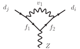
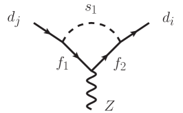
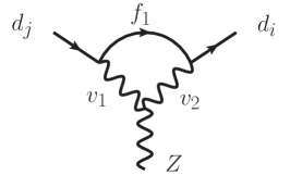
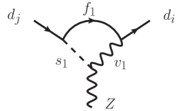
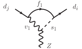
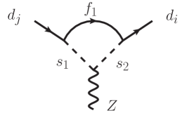
Figure 1: Representative Feynman diagrams contributing to the one-loop amputated $d_{j}-d_{i}-Z$ Green’s function. Straight lines denote fermions, wavy lines denotes vectors, and dashed lines denote scalar particles.

We present our result for the renormalised $Z$ penguin in the form of an effective vertex. The penguin function $C^{\sigma}_{d_{j}d_{i}Z}$ describing the transition between two light SM fermions $d_{j}\to d_{i}$ is defined in terms of the amputated vertex function as

$$\Gamma_{\mu\,\sigma}^{d_{j}d_{i}Z}=\gamma_{\mu}P_{\sigma}\times\frac{G_{F}}{\sqrt{2}}\frac{e}{\pi^{2}}M_{Z}^{2}\frac{c_{w}}{s_{w}}C^{\sigma}_{d_{j}d_{i}Z}\equiv\frac{\gamma_{\mu}P_{\sigma}}{(4\pi)^{2}}\hat{C}^{\sigma}_{d_{j}d_{i}Z}\,.$$ (4.1)

The function $C^{\sigma}_{d_{j}d_{i}Z}$, or $\hat{C}^{\sigma}_{d_{j}d_{i}Z}$ respectively, depends on all masses and couplings that appear; $\sigma=L,R$ stands for the chiral projection. It is obtained by calculating the Feynman diagrams shown in Fig. 1, using the Feynman rules derived from the Lagrangian Eq. (2.2). In the physical meson decay process, the momentum transfer is much smaller than any of the internal particle masses. Accordingly, setting the external momenta and light fermion masses to zero in the matching calculation, the result in the ’t Hooft-Feynman gauge is

$$\begin{split}&\hat{C}^{\sigma}_{d_{j}d_{i}Z}=\Bigg{\{}\sum_{f_{1}v_{1}}\sum_{f_{2}\notin\,\rm SM}\bigg{[}\kappa^{\sigma}_{f_{1}f_{2}v_{1}}B_{0}\big{(}m_{f_{1}},m_{v_{1}}\big{)}+\kappa^{\prime\sigma}_{f_{1}f_{2}v_{1}}\bigg{]}+\sum_{f_{1}s_{1}}\sum_{f_{2}\notin\,\rm SM}\kappa^{\sigma}_{f_{1}f_{2}s_{1}}B_{0}\big{(}m_{f_{1}},m_{s_{1}}\big{)}\\ &\quad+\sum_{f_{1}f_{2}v_{1}}\bigg{[}\tilde{k}^{\sigma}_{f_{1}f_{2}v_{1}}\Big{(}\tilde{C_{0}}\big{(}m_{f_{1}},m_{f_{2}},M_{v_{1}}\big{)}-\tfrac{1}{2}\Big{)}+k^{\sigma}_{f_{1}f_{2}v_{1}}C_{0}\big{(}m_{f_{1}},m_{f_{2}},M_{v_{1}}\big{)}+k^{\prime\sigma}_{f_{1}f_{2}v_{1}}\bigg{]}\\ &\quad+\sum_{f_{1}v_{1}v_{2}}\bigg{[}\tilde{k}^{\sigma}_{f_{1}v_{1}v_{2}}\Big{(}\tilde{C_{0}}\big{(}m_{f_{1}},M_{v_{1}},M_{v_{2}}\big{)}+\tfrac{1}{2}\Big{)}+k^{\sigma}_{f_{1}v_{1}v_{2}}C_{0}\big{(}m_{f_{1}},M_{v_{1}},M_{v_{2}}\big{)}+k^{\prime\sigma}_{f_{1}v_{1}v_{2}}\bigg{]}\\ &\quad+\sum_{f_{1}v_{1}s_{1}}\bigg{[}\tilde{k}^{\sigma}_{f_{1}v_{1}s_{1}}\Big{(}\tilde{C_{0}}\big{(}M_{s_{1}},m_{f_{1}},M_{v_{1}}\big{)}+\tfrac{1}{2}\Big{)}+k^{\sigma}_{f_{1}v_{1}s_{1}}C_{0}\big{(}M_{s_{1}},m_{f_{1}},M_{v_{1}}\big{)}\bigg{]}\\ &\quad+\sum_{f_{1}f_{2}s_{1}}\bigg{[}\tilde{k}^{\sigma}_{f_{1}f_{2}s_{1}}\Big{(}\tilde{C_{0}}\big{(}M_{s_{1}},m_{f_{1}},m_{f_{2}}\big{)}-\tfrac{1}{2}\Big{)}+k^{\sigma}_{f_{1}f_{2}s_{1}}C_{0}\big{(}M_{s_{1}},m_{f_{1}},m_{f_{2}}\big{)}\bigg{]}\\ &\quad+\sum_{f_{1}s_{1}s_{2}}\tilde{k}^{\sigma}_{f_{1}s_{1}s_{2}}\Big{(}\tilde{C_{0}}\big{(}M_{s_{1}},M_{s_{2}},m_{f_{1}}\big{)}+\tfrac{1}{2}\Big{)}\Bigg{\}}\,.\end{split}$$ (4.2)

The functions $C_{0}$ and $\tilde{C}_{0}$ can be found in Eqs. (B.2) and (B.3), respectively. The couplings are contained in the $\kappa$ and $k$ factors that are defined as follows:

$$\begin{split}\kappa^{\sigma}_{f_{1}f_{2}v_{1}}&=-\frac{m_{f_{1}}}{m_{f_{2}}}\bigg{(}g_{Z\bar{d}_{i}f_{2}}^{\sigma}\bigg{[}\bigg{(}4-\frac{m_{f_{1}}^{2}}{M_{v_{1}}^{2}}\bigg{)}g_{v_{1}\bar{f}_{2}f_{1}}^{\mkern 1.0mu\overline{\mkern-1.0mu\sigma\mkern-1.0mu}\mkern 1.0mu}+\frac{m_{f_{1}}m_{f_{2}}}{M_{v_{1}}^{2}}g_{v_{1}\bar{f}_{2}f_{1}}^{\sigma}\bigg{]}g_{\bar{v}_{1}\bar{f}_{1}d_{j}}^{\sigma}\\ &\mkern 60.0mu+g_{\bar{v}_{1}\bar{d}_{i}f_{1}}^{\sigma}\bigg{[}\bigg{(}4-\frac{m_{f_{1}}^{2}}{M_{v_{1}}^{2}}\bigg{)}g_{v_{1}\bar{f}_{1}f_{2}}^{\mkern 1.0mu\overline{\mkern-1.0mu\sigma\mkern-1.0mu}\mkern 1.0mu}+\frac{m_{f_{1}}m_{f_{2}}}{M_{v_{1}}^{2}}g_{v_{1}\bar{f}_{1}f_{2}}^{\sigma}\bigg{]}g_{Z\bar{f}_{2}d_{j}}^{\sigma}\bigg{)}\,,\\ \kappa^{\prime\sigma}_{f_{1}f_{2}v_{1}}&=\frac{2m_{f_{1}}}{m_{f_{2}}}\Big{(}g_{Z\bar{d}_{i}f_{2}}^{\sigma}g_{v_{1}\bar{f}_{2}f_{1}}^{\mkern 1.0mu\overline{\mkern-1.0mu\sigma\mkern-1.0mu}\mkern 1.0mu}g_{\bar{v}_{1}\bar{f}_{1}d_{j}}^{\sigma}+g_{v_{1}\bar{d}_{i}f_{1}}^{\sigma}g_{\bar{v}_{1}\bar{f}_{1}f_{2}}^{\mkern 1.0mu\overline{\mkern-1.0mu\sigma\mkern-1.0mu}\mkern 1.0mu}g_{Z\bar{f}_{2}d_{j}}^{\sigma}\Big{)}\,,\\ \end{split}$$ (4.3)

$$\begin{split}\kappa^{\sigma}_{f_{1}f_{2}s_{1}}&=\frac{m_{f_{1}}}{m_{f_{2}}}\Big{(}g_{Z\bar{d}_{i}f_{2}}^{\sigma}y_{s_{1}\bar{f}_{2}f_{1}}^{\sigma}y_{\bar{s}_{1}\bar{f}_{1}d_{j}}^{\sigma}+y_{s_{1}\bar{d}_{i}f_{1}}^{\mkern 1.0mu\overline{\mkern-1.0mu\sigma\mkern-1.0mu}\mkern 1.0mu}y_{\bar{s}_{1}\bar{f}_{1}f_{2}}^{\mkern 1.0mu\overline{\mkern-1.0mu\sigma\mkern-1.0mu}\mkern 1.0mu}g_{Z\bar{f}_{2}d_{j}}^{\sigma}\Big{)}\,,\\ \end{split}$$ (4.4)

$$\begin{split}\tilde{k}^{\sigma}_{f_{1}f_{2}v_{1}}&=\bigg{(}g_{Z\bar{f}_{2}f_{1}}^{\sigma}+\frac{m_{f_{1}}m_{f_{2}}}{2M_{v_{1}}^{2}}g_{Z\bar{f}_{2}f_{1}}^{\mkern 1.0mu\overline{\mkern-1.0mu\sigma\mkern-1.0mu}\mkern 1.0mu}\bigg{)}\,g_{\bar{v}_{1}\bar{d}_{i}f_{2}}^{\sigma}g_{v_{1}\bar{f}_{1}d_{j}}^{\sigma}\,,\\ k^{\sigma}_{f_{1}f_{2}v_{1}}&=-\frac{m_{f_{1}}m_{f_{2}}}{M_{v_{1}}^{2}}\,\big{(}m_{f_{1}}m_{f_{2}}g_{Z\bar{f}_{2}f_{1}}^{\sigma}+2M_{v_{1}}^{2}g_{Z\bar{f}_{2}f_{1}}^{\mkern 1.0mu\overline{\mkern-1.0mu\sigma\mkern-1.0mu}\mkern 1.0mu}\big{)}\,g_{\bar{v}_{1}\bar{d}_{i}f_{2}}^{\sigma}g_{v_{1}\bar{f}_{1}d_{j}}^{\sigma}\,,\\ k^{\prime\sigma}_{f_{1}f_{2}v_{1}}&=-g_{Z\bar{f}_{2}f_{1}}^{\sigma}g_{\bar{v}_{1}\bar{d}_{i}f_{2}}^{\sigma}g_{v_{1}\bar{f}_{1}d_{j}}^{\sigma}+\frac{1}{2}\big{(}g_{Z\bar{d}_{i}d_{i}}^{\sigma}g_{v_{1}\bar{d}_{i}f_{1}}^{\sigma}g_{\bar{v}_{1}\bar{f}_{1}d_{j}}^{\sigma}+g_{\bar{v}_{1}\bar{d}_{i}f_{1}}^{\sigma}g_{v_{1}\bar{f}_{1}d_{j}}^{\sigma}g_{Z\bar{d}_{j}d_{j}}^{\sigma}\big{)}\delta_{f_{1}f_{2}}\,,\\ \end{split}$$ (4.5)

$$\begin{split}\tilde{k}^{\sigma}_{f_{1}v_{1}v_{2}}&=-\bigg{(}3+\frac{m_{f_{1}}^{2}(M_{v_{1}}^{2}+M_{v_{2}}^{2}-M_{Z}^{2})}{4M_{v_{1}}^{2}M_{v_{2}}^{2}}\bigg{)}\,g_{Zv_{1}\bar{v}_{2}}g_{\bar{v}_{1}\bar{d}_{i}f_{1}}^{\sigma}g_{v_{2}\bar{f}_{1}d_{j}}^{\sigma}\\ &\quad-\frac{1}{2}\bigg{(}1+\frac{m_{f_{1}}^{2}}{2M_{v_{1}}^{2}}\bigg{)}\big{(}g_{Z\bar{d}_{i}d_{i}}^{\sigma}g_{v_{1}\bar{d}_{i}f_{1}}^{\sigma}g_{\bar{v}_{1}\bar{f}_{1}d_{j}}^{\sigma}+g_{v_{1}\bar{d}_{i}f_{1}}^{\sigma}g_{\bar{v}_{1}\bar{f}_{1}d_{j}}^{\sigma}g_{Z\bar{d}_{j}d_{j}}^{\sigma}\big{)}\delta_{v_{1}v_{2}}\,,\\ k^{\sigma}_{f_{1}v_{1}v_{2}}&=\frac{m_{f_{1}}^{2}\left(M_{v_{1}}^{4}+M_{v_{2}}^{4}-M_{Z}^{2}(M_{v_{1}}^{2}+M_{v_{2}}^{2})\right)}{M_{v_{1}}^{2}M_{v_{2}}^{2}}\,g_{Zv_{1}\bar{v}_{2}}g_{\bar{v}_{1}\bar{d}_{i}f_{1}}^{\sigma}g_{v_{2}\bar{f}_{1}d_{j}}^{\sigma}\,,\\ k^{\prime\sigma}_{f_{1}v_{1}v_{2}}&=2\,g_{Zv_{1}\bar{v}_{2}}g_{\bar{v}_{1}\bar{d}_{i}f_{1}}^{\sigma}g_{v_{2}\bar{f}_{1}d_{j}}^{\sigma}\,,\\ \end{split}$$ (4.6)

$$\begin{split}\tilde{k}^{\sigma}_{f_{1}v_{1}s_{1}}&=-\frac{k^{\sigma}_{f_{1}v_{1}s_{1}}}{4M_{v_{1}}^{2}}\,,\qquad k^{\sigma}_{f_{1}v_{1}s_{1}}=m_{f_{1}}\left(g_{Z\bar{v}_{1}s_{1}}y_{\bar{s}_{1}\bar{d}_{i}f_{1}}^{\mkern 1.0mu\overline{\mkern-1.0mu\sigma\mkern-1.0mu}\mkern 1.0mu}g_{v_{1}\bar{f}_{1}d_{j}}^{\sigma}+g_{Zv_{1}\bar{s}_{1}}y_{s_{1}\bar{f}_{1}d_{j}}^{\sigma}g_{\bar{v}_{1}\bar{d}_{i}f_{1}}^{\sigma}\right)\,,\\ \end{split}$$ (4.7)

$$\begin{split}\tilde{k}^{\sigma}_{f_{1}f_{2}s_{1}}&=\frac{1}{2}\,g_{Z\bar{f}_{2}f_{1}}^{\mkern 1.0mu\overline{\mkern-1.0mu\sigma\mkern-1.0mu}\mkern 1.0mu}y_{\bar{s}_{1}\bar{d}_{i}f_{2}}^{\mkern 1.0mu\overline{\mkern-1.0mu\sigma\mkern-1.0mu}\mkern 1.0mu}y_{s_{1}\bar{f}_{1}d_{j}}^{\sigma}\,,\qquad k^{\sigma}_{f_{1}f_{2}s_{1}}=-m_{f_{1}}m_{f_{2}}g_{Z\bar{f}_{2}f_{1}}^{\sigma}y_{\bar{s}_{1}\bar{d}_{i}f_{2}}^{\mkern 1.0mu\overline{\mkern-1.0mu\sigma\mkern-1.0mu}\mkern 1.0mu}y_{s_{1}\bar{f}_{1}d_{j}}^{\sigma}\,,\\ \end{split}$$ (4.8)

$$\begin{split}\tilde{k}^{\sigma}_{f_{1}s_{1}s_{2}}&=\frac{1}{2}\,g_{Z\bar{s}_{1}s_{2}}y_{\bar{s}_{2}\bar{d}_{i}f_{1}}^{\mkern 1.0mu\overline{\mkern-1.0mu\sigma\mkern-1.0mu}\mkern 1.0mu}y_{s_{1}\bar{f}_{1}d_{j}}^{\sigma}-\frac{1}{4}\Big{(}g_{Z\bar{d}_{i}d_{i}}^{\sigma}y_{\bar{s}_{1}\bar{d}_{i}f_{1}}^{\mkern 1.0mu\overline{\mkern-1.0mu\sigma\mkern-1.0mu}\mkern 1.0mu}y_{s_{1}\bar{f}_{1}d_{j}}^{\sigma}+y_{\bar{s}_{1}\bar{d}_{i}f_{1}}^{\mkern 1.0mu\overline{\mkern-1.0mu\sigma\mkern-1.0mu}\mkern 1.0mu}y_{s_{1}\bar{f}_{1}d_{j}}^{\sigma}g_{Z\bar{d}_{j}d_{j}}^{\sigma}\Big{)}\delta_{s_{1}s_{2}}\,.\end{split}$$ (4.9)

The sums in (4.2) run over all components of the fields (e.g., explicitly over $W^{+}$ and $W^{-}$ in the SM). Note that the scalar-index sums in (4.2) run only over physical fields; the contributions of would-be Goldstone bosons have been accounted for via the replacement of the Goldstone couplings in terms of couplings to physical particles, using Eq. (3.6). The contribution of the $Z$ penguin to processes like rare $B$ and $K$ decays is not separately gauge-invariant without including the box contributions. We present the explicit generic results for completeness in Appendix A.

Our result (4.1) consists of several contributions. In general, we can write ($i\neq j$)

$$\begin{split}\Gamma_{\mu\,\sigma}^{d_{j}d_{i}Z}=\Gamma_{\mu\,\sigma}^{d_{j}d_{i}Z,(1)}+\Big{[}\delta Z_{Z\bar{d}_{i}d_{j}}^{g,\sigma}+\tfrac{1}{2}{\textstyle\sum\limits_{f_{1}}}\Big{(}g_{Z\bar{d}_{i}f_{1}}^{\sigma}\delta Z_{\bar{f}_{1}d_{j}}^{\psi,\sigma}+\delta Z_{\bar{d}_{i}f_{1}}^{\psi,\sigma\,\dagger}g_{Z\bar{f}_{1}d_{j}}^{\sigma}\Big{)}+\tfrac{1}{2}{\textstyle\sum\limits_{v_{1}}}\delta Z_{Zv_{1}}^{V}g_{\bar{v}_{1}\bar{d}_{i}d_{j}}^{\sigma}\Big{]}P_{\sigma}\,.\end{split}$$ (4.10)

Here $\Gamma_{\mu\,\sigma}^{Zd_{j}d_{i},(1)}$ denotes the sum of all contributing one-loop diagrams, and the rest are the vertex, fermion field, and gauge-boson field renormalisation constants, respectively. Note that in this work we assume the absence of tree-level FCNC transitions between light quarks, i.e. $g_{\bar{v}_{1}\bar{d}_{i}d_{j}}^{\sigma}=0$. In this case, we can use the STIs (3.8), (3.9) and (3.10) to show that the fermion field renormalisation constants are sufficient to cancel all divergences in (4.10) (in other words, $\delta Z_{Z\bar{d}_{i}d_{j}}^{g,\sigma}$ can be chosen to vanish). This is done explicitly in Sec. 5.

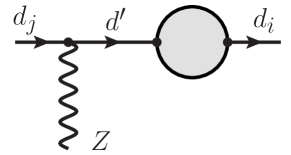
Figure 2: One-heavy-particle reducible contribution to the $Z$ penguin.

The two-point functions in the full theory lead to mixing among the fermions beyond tree level. We perform an off-diagonal field renormalisation for all fermions fields, with finite terms chosen to restore a diagonal and canonically normalised kinetic and mass term. As one consequence, diagrams with a reducible heavy-fermion line (of the form shown in Figure 2) are exactly cancelled by corresponding counterterm diagrams.

The one-loop corrections to the renormalised fermion two-point function can be written as

$$\delta\Gamma_{\sigma}^{f_{i}f_{j}}=\Big{[}\big{(}\Sigma_{V,\bar{f}_{j}f_{i}}^{\psi,\sigma}+\delta Z_{H,\bar{f}_{j}f_{i}}^{\psi,\sigma}\big{)}\not{p}+\Sigma_{S,\bar{f}_{j}f_{i}}^{\psi,\sigma}-\tfrac{1}{2}(m_{f_{j}}\delta Z_{\bar{f}_{j}f_{i}}^{\psi,\sigma}+\delta Z_{\bar{f}_{j}f_{i}}^{\psi,\mkern 1.0mu\overline{\mkern-1.0mu\sigma\mkern-1.0mu}\mkern 1.0mu\,\dagger}m_{f_{i}})-\delta_{ji}\delta m_{f_{i}}\Big{]}P_{\sigma}\,.$$ (4.11)

The finite parts of the field renormalisation constants for $j\neq i$ are obtained from the requirement that the off-diagonal parts of the self energy (4.11) vanish. They are given by

$$\delta Z_{\bar{f}_{j}f_{i}}^{\psi,\sigma}\big{|}_{\rm fin}=\frac{2}{m_{f_{j}}^{2}-m_{f_{i}}^{2}}\Big{(}m_{f_{i}}^{2}\Sigma_{V,\bar{f}_{j}f_{i}}^{\psi,\sigma}+m_{f_{j}}m_{f_{i}}\Sigma_{V,\bar{f}_{j}f_{i}}^{\psi,\mkern 1.0mu\overline{\mkern-1.0mu\sigma\mkern-1.0mu}\mkern 1.0mu}+m_{f_{j}}\Sigma_{S,\bar{f}_{j}f_{i}}^{\psi,\sigma}+m_{f_{i}}\Sigma_{S,\bar{f}_{j}f_{i}}^{\psi,\mkern 1.0mu\overline{\mkern-1.0mu\sigma\mkern-1.0mu}\mkern 1.0mu}\Big{)}\big{|}_{\rm fin}\,.$$ (4.12)

They enter our generic result after having been expanded in small mass ratios. The diagonal field renormalisation constants are not necessary in our case. If we had allowed for the presence of tree-level $d_{j}\to d_{i}$ transitions, one would have to fix these constants by renormalisation conditions. Note that, in this case, the one-loop result would correspond to a tiny correction of an already suppressed tree-level amplitude. These consideration can be important, however, in an analogous treatment of charged current couplings [24].

We will show in the next section that all divergences in our generic result completely cancel against the divergent terms in the field rotation, without introducing additional counterterms. In order to make this cancellation manifest, it is necessary to use the consequences of tree-level perturbative unitarity derived in Sec. 2 in form of the STIs. This step is independent of the specification of a model and can be applied without detailed knowledge about the sector responsible for the spontaneous symmetry breaking.

5 Renormalised Results

The result (4.2) is valid for any number of heavy new scalars, vectors, and Dirac fermions. It is, however, not very suitable for numerical evaluation: the functions $\tilde{C_{0}}$ in Eq. (5.4) contain divergent terms (cf. Appendix B). While the STI (via relations between the couplings appearing in the coefficients (4.3) - (4.9)) ensure that the result is finite, the cancellation of the divergences is not manifest. In this section we will derive manifestly finite versions of our result that, in addition, depend on a minimal number of physical couplings.

In order to make contact to phenomenological applications, we remind the reader that the loop functions appearing in rare $K$ and $B$ meson decays are given by the following combinations [25]

$$\begin{split}X^{\sigma}(x)=C_{sdZ}^{\sigma}(x)-4B_{sd\nu\nu}^{\sigma L}(x)\,,\quad Y^{\sigma\sigma^{\prime}}(x)=C_{sdZ}^{\sigma}(x)-B(x)_{sd\ell\ell}^{\sigma\sigma^{\prime}}\,,\end{split}$$ (5.1)

with $C_{sdZ}^{\sigma}$ and $B_{sd\ell_{k}\ell_{k}}^{\sigma\sigma^{\prime}}$ given in Eq. (4.1) and Eq. (A.2), respectively.

5.1 SM Fermions and charged scalars and vectors

We first consider the simplified case of theories with charged heavy scalars and vectors – in other words, we drop all coefficients in Eq. (4.2) that involve couplings to heavy new fermions. We then simplify the remaining expression by repeatedly eliminating physical coupling constants via application of the STI. The result obtained in this way is not only manifestly finite, but also depends on fewer physical coupling constants than the original expression. This procedure is not unique. While the STI ensure that one will finally arrive at a finite result, there is some freedom of which couplings to eliminate and which ones to retain.

For instance, continuing with our simplified case, we can first eliminate the right-handed $Z$-fermion coupling by solving the “Yukawa sum rule” Eq. (3.10) for $g_{Z\bar{q}q}^{R}$, and solving the “gauge boson mass sum rule” Eq. (3.9) for $g_{Z\bar{t}t}^{R}$. We then apply the “unitarity sum rule”, Eq. (3.8), together with the universality of the $Z$ coupling to fermions, to eliminate all dependence on couplings involving light quarks (this step is a generalization of the GIM mechanism). We can then solve Eq. (3.8) for $g_{Z\bar{t}t}^{L}$. Applying the resulting relations to Eqs. (4.3)-(4.9) eliminates all divergences, and we obtain the manifestly finite expression

$$\begin{split}\hat{C}^{L}_{d_{j}d_{i}Z}=&\sum_{s_{1}s_{2}}f_{S}(m_{t},M_{s_{1}},M_{s_{2}})y_{s_{2}^{+}\bar{t}d_{j}}^{L}\left(\delta_{s_{1}s_{2}}y_{s_{2}^{-}\bar{d_{i}}t}^{R}\left(g_{Z\bar{d_{j}}d_{j}}^{L}-g_{Z\bar{t}t}^{L}\right)+g_{Zs_{1}^{+}s_{2}^{-}}y_{s_{1}^{-}\bar{d_{i}}t}^{R}\right)\\ &+\sum_{v_{1}v_{2}}f_{V}(m_{t},M_{v_{1}},M_{v_{2}})g_{Zv_{2}^{+}v_{1}^{-}}g_{v_{1}^{+}\bar{t}d_{j}}^{L}g_{v_{2}^{-}\bar{d_{i}}t}^{L}\\ &+\sum_{s_{1}v_{1}}f_{VS}(m_{t},M_{s_{1}},M_{v_{1}})y_{s_{1}^{+}\bar{t}d_{j}}^{L}g_{v_{1}^{-}\bar{d_{i}}t}^{L}g_{Zv_{1}^{+}s_{1}^{-}}\\ &+\sum_{s_{1}v_{1}}f_{VS^{\prime}}(m_{t},M_{s_{1}},M_{v_{1}})y_{s_{1}^{-}\bar{d_{i}}t}^{R}g_{v_{1}^{+}\bar{t}d_{j}}^{L}g_{Zv_{1}^{-}s_{1}^{+}}\,.\end{split}$$ (5.2)

The loop functions are given by

$$\begin{split}f_{V}(m_{i},m_{j},m_{k})&=m_{i}^{2}C_{0}\left(m_{i},m_{k},m_{k}\right)-\frac{m_{i}^{2}\left(m_{j}^{2}+m_{k}^{2}-M_{Z}^{2}\right)}{4m_{j}^{2}m_{k}^{2}}\\ &+\frac{m_{i}^{2}\left(-3m_{j}^{2}+m_{k}^{2}-M_{Z}^{2}\right)+4m_{k}^{2}\left(m_{j}^{2}-m_{k}^{2}+M_{Z}^{2}\right)}{4m_{j}^{2}m_{k}^{2}}m_{i}^{2}C_{0}\left(m_{i},m_{i},m_{k}\right)\\ &+\frac{-M_{Z}^{2}\left(3m_{j}^{2}+4m_{k}^{2}\right)-13m_{j}^{2}m_{k}^{2}+3m_{j}^{4}+4m_{k}^{4}}{4m_{j}^{2}m_{k}^{2}}m_{i}^{2}C_{0}\left(m_{i},m_{j},m_{k}\right)\,,\\ f_{S}(m_{i},m_{j},m_{k})&=\frac{1}{2}m_{i}^{2}C_{0}\left(m_{i},m_{i},m_{k}\right)-\frac{1}{2}m_{j}^{2}C_{0}\left(m_{i},m_{j},m_{k}\right)-\frac{1}{2}\,,\\ f_{VS}(m_{i},m_{j},m_{k})&=m_{i}\left(1-\frac{m_{j}^{2}}{4m_{k}^{2}}\right)C_{0}\left(m_{i},m_{j},m_{k}\right)\\ &+\left(\frac{m_{i}^{3}}{4m_{k}^{2}}-m_{i}\right)C_{0}\left(m_{i},m_{i},m_{k}\right)-\frac{m_{i}}{4m_{k}^{2}}\,,\\ f_{VS^{\prime}}(m_{i},m_{j},m_{k})&=\frac{m_{i}^{3}C_{0}\left(m_{i},m_{i},m_{j}\right)}{4m_{k}^{2}}+\frac{3}{4}m_{i}C_{0}\left(m_{i},m_{j},m_{k}\right)-\frac{m_{i}}{4m_{k}^{2}}\,.\end{split}$$ (5.3)

The function $C_{0}$ can be found in Eq. (B.2).

A comment is in order: The sums over charged vectors $v_{i}$ and charged scalars $s_{i}$ in Eq. (5.2) run over the particle types, but not over the different charges: for SM fermion content the charge of the internal vectors and scalars is fixed by the external fermions (e.g., for a strange to down transition, there are only up-type quarks in the loop, so the internal vectors and scalars must have negative charge $-e$).

5.1.1 Standard Model

We illustrate the general procedure described above by considering the $s\to d$ transition in the SM. Here, the only relevant heavy degrees of freedom are the top quark, and the gauge bosons $Z$ and $W^{\pm}$. Starting with the general result (4.2), we need to keep only the terms

$$\begin{split}\hat{C}^{L,\text{SM}}_{sdZ}=&\sum_{f_{1}f_{2}v_{1}}\bigg{[}\tilde{k}^{\sigma}_{f_{1}f_{2}v_{1}}\Big{(}\tilde{C_{0}}\big{(}m_{f_{1}},m_{f_{2}},M_{v_{1}}\big{)}-\tfrac{1}{2}\Big{)}+k^{\sigma}_{f_{1}f_{2}v_{1}}C_{0}\big{(}m_{f_{1}},m_{f_{2}},M_{v_{1}}\big{)}+k^{\prime\sigma}_{f_{1}f_{2}v_{1}}\bigg{]}\\ +&\sum_{f_{1}v_{1}v_{2}}\bigg{[}\tilde{k}^{\sigma}_{f_{1}v_{1}v_{2}}\Big{(}\tilde{C_{0}}\big{(}m_{f_{1}},M_{v_{1}},M_{v_{2}}\big{)}+\tfrac{1}{2}\Big{)}+k^{\sigma}_{f_{1}v_{1}v_{2}}C_{0}\big{(}m_{f_{1}},M_{v_{1}},M_{v_{2}}\big{)}+k^{\prime\sigma}_{f_{1}v_{1}v_{2}}\bigg{]}\,\end{split}$$ (5.4)

Next, we insert the SM couplings of $W$ bosons

$$g^{L}_{W^{+}\bar{u}_{j}d_{k}}=\frac{e}{s_{w}\sqrt{2}}V_{jk}\,,\qquad g^{L}_{W^{+}\bar{\nu}_{j}\ell_{k}}=\frac{e}{s_{w}\sqrt{2}}\delta_{jk}\,,\qquad g_{ZW^{+}W^{-}}=\frac{e}{t_{w}}$$ (5.5)

and $Z$ bosons

$$g^{L}_{Z\bar{f}_{j}f_{k}}=\frac{2e}{s_{2w}}\left(T_{3}^{f}-Q_{f}s_{w}^{2}\right)\delta_{jk}\,,\qquad g^{R}_{Z\bar{f}_{j}f_{k}}=-\frac{2e}{s_{2w}}Q_{f}s_{w}^{2}\delta_{jk}\,.$$ (5.6)

Here $T_{3}^{f}=\pm 1/2$ is the third component of the weak isospin of the fermion $f$ and $Q_{f}$ is its electric charge in units of the positron charge $e$. The sine of the weak mixing angle is denoted by $s_{w}=\sin(\theta_{w})$. In addition we defined $s_{2w}=\sin(2\theta_{w})$ and $t_{w}=\tan(\theta_{w})$. The CKM matrix elements are denoted by $V_{jk}$.

The $Z$-boson coupling to fermions in the SM is universal and diagonal; hence, the sum rule (3.8) leads to the unitarity of the CKM matrix. Defining $\lambda_{q}^{(d^{\prime}d)}=V_{qd^{\prime}}V_{qd}^{*}$, this allows us to eliminate $\lambda_{u}^{sd}=-\lambda_{c}^{sd}-\lambda_{t}^{sd}$, and thus the coefficient $\lambda_{t}^{sd}$ multiplies the difference of the diagrams with massive top and massless up quark. This leads to a partial cancellation of UV divergences – the well-known GIM (Glashow-Iliopoulos-Maiani) mechanism.

After this manipulation, the result still has a left-over divergence, proportional to

$$\frac{1}{M_{W}^{2}}-\frac{1}{c_{w}^{2}M_{Z}^{2}}\,.$$ (5.7)

Evaluating the sum rule (3.9) for the choice $\sigma=L$, $v_{1}=Z$, $v_{2}=W^{+}$, $f_{1}=t$, $f_{2}=b$, and inserting the SM couplings, leads immediately to the relation

$$M_{W}^{2}=c_{w}^{2}M_{Z}^{2}\,.$$ (5.8)

Thus, the divergent term vanishes. The finite term exactly reproduces the result of Inami and Lim [26]

$$C^{L\,(\rm SM)}_{d^{\prime}dZ}=\lambda_{t}^{(d^{\prime}d)}\,C(x_{t})\,,\quad C(x)=\frac{x}{8}\bigg{[}\frac{x-6}{x-1}+\frac{3x+2}{(x-1)^{2}}\log(x)\bigg{]}\,,$$ (5.9)

for the top-quark contribution to the $d^{\prime}\to dZ$ vertex. The ratio of the quark and $W$-boson masses squared is denoted by $x_{q}=m_{q}^{2}/M_{W}^{2}$.

Of course, the same result is obtained in a much simpler way by directly using the result (5.2). Both the GIM mechanism and “gauge boson mass relation” (5.8) are already built in. Moreover, it suffices to specify the reduced set of SM couplings (5.5) – the $Z$-fermion couplings (5.6) are then fixed via the STI.

5.1.2 2HDM

As an example with additional charged scalars we consider the contribution of charged Higgs bosons in a two Higgs doublet model (2HDM) [27]. Using that the couplings involving both charged gauge and Higgs bosons vanish, $g_{ZW_{j}^{+}h_{i}^{-}}=g_{ZW_{j}^{-}h_{i}^{+}}=0$, we see that only the first line in Eq. (5.2) contributes, with a prefactor given by

$$y_{h_{j}^{+}\bar{t}d}^{L}\left(\delta_{ij}y_{h_{j}^{-}\bar{s}t}^{R}\left(g_{Z\bar{d}d}^{L}-g_{Z\bar{t}t}^{L}\right)+g_{Zh_{i}^{+}h_{j}^{-}}y_{h_{i}^{-}\bar{s}t}^{R}\right)\,.$$ (5.10)

Specializing to the case of one charged Higgs, we need the following additional Feynman rules [27]

$$g_{Zh^{-}h^{+}}=-e\frac{c_{2w}}{2s_{w}c_{w}}\,,\quad y_{h^{+}\bar{t}d_{i}}^{L}=\big{(}y_{h^{-}\bar{d_{i}}t}^{R}\big{)}^{*}=\frac{m_{t}}{t_{\beta}}\frac{V_{td}e}{\sqrt{2}s_{w}M_{W}}\,,\quad y_{h^{+}\bar{t}d_{i}}^{R}=\big{(}y_{h^{-}\bar{d_{i}}t}^{L}\big{)}^{*}={\mathcal{O}}(m_{d_{i}})\,,$$ (5.11)

with $t_{\beta}=\tan\beta$. We then find

$$C(x_{t},y_{t})=-\frac{V_{td}V_{ts}^{*}}{8t_{\beta}^{2}}\,x_{t}\,f_{S}(m_{t},M_{h},M_{h})$$ (5.12)

where

$$f_{S}(m_{t},M_{h},M_{h})=\frac{y_{t}}{1-y_{t}}+\frac{y_{t}\log y_{t}}{(y_{t}-1)^{2}}$$ (5.13)

and we defined $x=m_{t}^{2}/M_{W}^{2}$, $y=m_{t}^{2}/M_{h}^{2}$. This reproduces the function

$$C_{H}(x_{t},y_{t})=-\frac{1}{8}|Y|^{2}x_{t}y_{t}\bigg{[}\frac{1}{1-y_{t}}+\frac{\log y_{t}}{(y_{t}-1)^{2}}\bigg{]}$$ (5.14)

from [28], where $Y=v_{1}/v_{2}=\cot\beta$.

5.2 Arbitrary charged Fermions, Scalars, and Vectors

We now consider the general case of theories with arbitrary numbers of heavy charged fermions, scalars and vectors, and simplify the general result Eq. (4.2) by repeatedly eliminating physical coupling constants via application of the STI.

In analogy to our procedure described in the previous section, we can first eliminate the diagonal right-handed $Z$-fermion coupling by solving the “Yukawa sum rule” Eq. (3.10) for $g_{Z\bar{f}f}^{R}$, thus eliminating this coupling in conjunction with couplings to heavy scalars. Next, we solve the “gauge boson mass sum rule” Eq. (3.9) for $g_{Z\bar{f}f}^{R}$ and use the resulting relation to eliminate all diagonal right-handed $Z$ couplings to fermions in conjunction with vector couplings. We then repeatedly apply the “unitarity sum rule”, Eq. (3.8), to eliminate all couplings of fermions to the charged vectors and all couplings of the $Z$ boson to left-handed fermions, looping over all heavy fermions. Together with our assumption of universality and diagonality of the $Z$-boson couplings to down-type SM quarks, this eliminates all divergences. Note that the “unitarity sum rule”, Eq. (3.8), leads to a “generalized GIM mechanism”, effectively eliminating some of the couplings of one (arbitrarily chosen) heavy fermions in the loop (denoted below by the subscript $f^{\prime}$). The resulting, manifestly finite expression for the $Z$ penguin for an arbitrary number of charged fermions, scalars, and vectors is then

$$\begin{split}\hat{C}_{d_{j}d_{i}Z}^{L}=&\quad\sum_{f_{1}f_{2}v_{1}}g_{Z\bar{f}_{2}f_{1}}^{L}g_{v_{1}\bar{f}_{1}d_{j}}^{L}g_{\bar{v}_{1}\bar{d_{i}}f_{2}}^{L}F_{V}\left(m_{f_{1}},m_{f_{2}},M_{v_{1}}\right)\\ &+\sum_{f_{1}f_{2}v_{1}}g_{Z\bar{f}_{2}f_{1}}^{R}g_{v_{1}\bar{f}_{1}d_{j}}^{L}g_{\bar{v}_{1}\bar{d_{i}}f_{2}}^{L}F_{V^{\prime}}\left(m_{f_{1}},m_{f_{2}},M_{v_{1}}\right)\\ &+\sum_{f_{1}v_{1}v_{2}}g_{Zv_{2}\bar{v}_{1}}g_{v_{1}\bar{f}_{1}d_{j}}^{L}g_{\bar{v}_{2}\bar{d_{i}}f_{1}}^{L}F_{V^{\prime\prime}}\left(m_{f^{\prime}},m_{f_{1}},M_{v_{1}},M_{v_{2}}\right)\\ &+\sum_{f_{1}f_{2}s_{1}}g_{Z\bar{f}_{2}f_{1}}^{L}y_{s_{1}\bar{f}_{1}d_{j}}^{L}y_{\bar{s}_{1}\bar{d_{i}}f_{2}}^{R}F_{S}\left(m_{f_{1}},m_{f_{2}},M_{s_{1}}\right)\\ &+\sum_{f_{1}s_{1}s_{2}}\left(g_{Zs_{2}\bar{s}_{1}}+\delta_{s_{1}s_{2}}g_{Z\bar{d}_{j}d_{j}}^{L}\right)y_{s_{1}\bar{f}_{1}d_{j}}^{L}y_{\bar{s}_{2}\bar{d_{i}}f_{1}}^{R}F_{S^{\prime}}\left(m_{f_{1}},M_{s_{1}},M_{s_{2}}\right)\\ &+\sum_{f_{1}f_{2}s_{1}}g_{Z\bar{f}_{2}f_{1}}^{R}y_{s_{1}\bar{f}_{1}d_{j}}^{L}y_{\bar{s}_{1}\bar{d_{i}}f_{2}}^{R}F_{S^{\prime\prime}}\left(m_{f_{1}},m_{f_{2}},M_{s_{1}}\right)\\ &+\sum_{f_{1}s_{1}v_{1}}g_{Zv_{1}\bar{s}_{1}}y_{s_{1}\bar{f}_{1}d_{j}}^{L}g_{\bar{v}_{1}\bar{d_{i}}f_{1}}^{L}F_{\text{SV}}\left(m_{f_{1}},M_{s_{1}},M_{v_{1}}\right)\\ &+\sum_{f_{1}s_{1}v_{1}}g_{Z\bar{v}_{1}s_{1}}g_{v_{1}\bar{f}_{1}d_{j}}^{L}y_{\bar{s}_{1}\bar{d_{i}}f_{1}}^{R}F_{\text{SV}^{\prime}}\left(m_{f_{1}},M_{s_{1}},M_{v_{1}}\right)\,,\end{split}$$ (5.15)

The respective loop functions can be written

$$\begin{split}&F_{V}\left(m_{i},m_{j},m_{k}\right)=\tilde{C}_{\delta}\left(m_{i},m_{j},m_{k}\right)+\frac{m_{j}^{2}}{m_{k}^{2}}\left(m_{j}^{2}C_{0}\left(m_{j},m_{j},m_{k}\right)-m_{i}^{2}C_{0}\left(m_{i},m_{j},m_{k}\right)\right)\,,\\ &F_{V^{\prime}}\left(m_{i},m_{j},m_{k}\right)=\frac{m_{i}m_{j}}{2m_{k}^{2}}\left(\tilde{C}_{\delta}\left(m_{i},m_{j},m_{k}\right)-4m_{k}^{2}C_{\delta}\left(m_{i},m_{j},m_{k}\right)\right)\,,\\ &F_{V^{\prime\prime}}(m_{i},m_{j},m_{k},m_{l})=\tilde{C}_{\Delta}(m_{i},m_{j},m_{k},m_{l})+f_{V^{\prime\prime}}(m_{i},m_{k},m_{l})-f_{V^{\prime\prime}}(m_{j},m_{k},m_{l})\,,\\ &F_{S}\left(m_{i},m_{j},m_{k}\right)=-m_{i}m_{j}C_{0}\left(m_{i},m_{j},m_{k}\right)\,,\\ &F_{S^{\prime}}\left(m_{i},m_{j},m_{k}\right)=-\frac{1}{2}\left(\tilde{C}_{\delta}\left(m_{j},m_{i},m_{k}\right)+1\right)\,,\\ &F_{S^{\prime\prime}}\left(m_{i},m_{j},m_{k}\right)=\frac{1}{2}\tilde{C}_{\delta}\left(m_{i},m_{j},m_{k}\right)\,,\\ &F_{\text{SV}}\left(m_{i},m_{j},m_{k}\right)=\frac{m_{i}}{4m_{k}^{2}}\left(4m_{k}^{2}C_{\delta}\left(m_{j},m_{i},m_{k}\right)-\tilde{C}_{\delta}\left(m_{j},m_{i},m_{k}\right)-1\right)\,,\\ &F_{\text{SV}^{\prime}}\left(m_{i},m_{j},m_{k}\right)=\frac{m_{i}}{4m_{k}^{2}}\left(4m_{k}^{2}C_{0}\left(m_{i},m_{j},m_{k}\right)-\tilde{C}_{\delta}\left(m_{k},m_{i},m_{j}\right)-1\right)\,,\\ \end{split}$$ (5.16)

where

$$\begin{split}\frac{1}{m_{i}^{2}}f_{V^{\prime\prime}}(m_{i},m_{j},m_{k})&=\frac{m_{j}^{2}+m_{k}^{2}-M_{Z}^{2}}{4m_{j}^{2}m_{k}^{2}}\big{(}1+\tilde{C}_{\delta}(m_{j},m_{i},m_{k})\big{)}\\ &+\left(\frac{m_{i}^{2}}{m_{k}^{2}}+\frac{m_{k}^{2}-M_{Z}^{2}}{m_{j}^{2}}+1\right)C_{0}(m_{i},m_{i},m_{k})\\ &-\frac{m_{j}^{4}+m_{k}^{4}-M_{Z}^{2}\left(m_{j}^{2}+m_{k}^{2}\right)}{m_{j}^{2}m_{k}^{2}}C_{0}(m_{i},m_{j},m_{k})\end{split}$$ (5.17)

and

$$\begin{split}\tilde{C}_{\Delta}\left(m_{i},m_{j},m_{k},m_{l}\right)&=3\left(\tilde{C}_{0}\left(m_{i},m_{k},m_{l}\right)-\tilde{C}_{0}\left(m_{j},m_{k},m_{l}\right)\right)\\ &\quad-\tilde{C}_{0}\left(m_{i},m_{i},m_{l}\right)+\tilde{C}_{0}\left(m_{j},m_{j},m_{l}\right)\\ \tilde{C}_{\delta}(m_{i},m_{j},m_{k})&=\tilde{C}_{0}\left(m_{i},m_{j},m_{k}\right)-\tilde{C}_{0}\left(m_{j},m_{j},m_{k}\right)\\ C_{\delta}(m_{i},m_{j},m_{k})&=C_{0}\left(m_{i},m_{j},m_{k}\right)-C_{0}\left(m_{j},m_{j},m_{k}\right)\,.\end{split}$$ (5.18)

These loop functions are manifestly finite; it is interesting to note that one could perform the whole calculation without regulator in four space-time dimensions if one applies the sum rules first. Note also that several of the loop functions vanish if the fermion masses are equal; namely, we have

$$F_{V}\left(m,m,M\right)=F_{V^{\prime}}\left(m,m,M\right)=F_{V^{\prime\prime}}\left(m,m,M\right)=F_{S^{\prime\prime}}\left(m,m,M\right)=0\,.$$ (5.19)

As a consequence, the result depends only the off-diagonal right-handed couplings of the $Z$ boson to fermions. Furthermore, we have $F_{S}\left(m,m,M\right)=F_{S^{\prime}}\left(m,M,M\right)$, and the only contributions in the fourth line in Eq. (5.15) proportional to diagonal $Z$ couplings arise from the finite parts of the field renormalisation constants.

As before, given the charges of the internal fermions, the charges of the internal scalars and vectors are determined by the charges of the external particles, via $Q_{s,v}=1/3+Q_{f}$; so the sums in Eq. (5.15) effectively run only over the particles with positive charge. Finally, we remind the reader that we suppressed colour indices throughout; coloured particles can easily be taken into account with the understanding that the sums also run over all components of fields in multiplets of $SU(3)$.

5.2.1 Vector-like quarks

As an example, we consider vector-like quarks in a representation that does not generate tree-level FCNC transitions in the down-quark sector [29]. For simplicity, we treat the case of an up-type singlet vector-like quark, $U$, with charge $2/3$, isospin zero, and mass $m_{U}$.

The additional quark $U$ mixes with the SM fermions via Yukawa term in the Lagrangian, given by

$$\mathcal{L}_{Y}=-\sum_{k}\overline{Q}_{L}^{k}Y_{k}^{U}U_{R}\tilde{H}+\text{h.c.}\,$$ (5.20)

(note that hard mixing terms $\mathcal{L}_{\text{mix}}=-\sum_{k=1}^{3}m_{uu}^{k}\,\overline{u}_{R}^{k}U_{L}+\text{h.c.}$ can be eliminated via a field rotation). Here $k$ is a SM generation index, and the charge conjugate of the Higgs field $H$ is given by $\tilde{H}=i\sigma^{2}H^{*}=i\sigma^{2}(H^{\dagger})^{T}$.

We obtain the contributions to the $Z$ penguin by inserting the appropriate couplings into the general result (5.15). First, note that all RH $Z$ couplings as well as the LH tree-level $Z$ couplings to down-type quarks are not changed from their SM values. Therefore, we need only the following additional Feynman rules:

$$\begin{split}g_{Z\bar{u}_{i}u_{j}}^{L}=\frac{e}{s_{w}c_{w}}\bigg{[}\frac{1}{2}(VV^{\dagger})_{ij}-\frac{2}{3}s_{w}^{2}\delta_{ij}\bigg{]}\,,\quad g_{W^{+}\bar{u}_{i}d_{j}}^{L}=\frac{e}{\sqrt{2}s_{w}}V_{ij}\,,\quad g_{ZW^{+}W^{-}}=\frac{ec_{w}}{s_{w}}\end{split}$$ (5.21)

where $V$ is the generalized, non-unitary CKM matrix (see, e.g., [30, 31]). (Note that the Higgs couplings contribute only indirectly to the $Z$ penguin, via the mixing angles comprised by the matrix $V$.) The resulting expression for the $Z$ penguin is

$$\begin{split}C&=V_{td}V_{ts}^{*}f_{1}(x_{t})+V_{Ud}V_{Us}^{*}f_{1}(y_{U})+V_{Ud}V_{ts}^{*}(VV^{\dagger})_{tU}f_{4}(x_{t},y_{U})+V_{td}V_{Us}^{*}(VV^{\dagger})_{Ut}f_{4}(y_{U},x_{t})\\ &+V_{td}\big{[}V_{cs}^{*}(VV^{\dagger})_{ct}+V_{us}^{*}(VV^{\dagger})_{ut}\big{]}f_{2}(x_{t})+V_{Ud}\big{[}V_{cs}^{*}(VV^{\dagger})_{cU}+V_{us}^{*}(VV^{\dagger})_{uU}\big{]}f_{2}(y_{U})\\ &+V_{ts}^{*}\big{[}V_{cd}(VV^{\dagger})_{tc}+V_{ud}(VV^{\dagger})_{tu}\big{]}f_{3}(x_{t})+V_{Us}^{*}\big{[}V_{cd}(VV^{\dagger})_{Uc}+V_{ud}(VV^{\dagger})_{Uu}\big{]}f_{3}(y_{U})\end{split}$$ (5.22)

where $x_{t}=m_{t}^{2}/M_{W}^{2}$, $y_{U}=m_{U}^{2}/M_{W}^{2}$, and the loop functions are given by

$$\begin{split}f_{1}(x)&=\frac{x(x-6)}{8(x-1)}+\frac{x(2+3x)\log x}{8(x-1)^{2}}\,,\quad f_{2}(x)=\frac{x\log x}{8(1-x)}\,,\quad f_{3}(x)=-\frac{x}{8}-f_{2}(x)\,,\\[5.69054pt] f_{4}(x,y)&=\frac{x(x-2y+xy)\log x}{8(x-1)(x-y)}-\frac{(x-1)y^{2}\log y}{8(y-1)(x-y)}-\frac{x}{8}\,.\end{split}$$ (5.23)

The box contribution for external neutrinos (needed for the rare $K\to\pi\nu\bar{\nu}$ decays) is

$$B=V_{td}V_{ts}^{*}\,g(x_{t})+V_{Ud}V_{Us}^{*}\,g(y_{U})$$ (5.24)

where

$$g(x)=\frac{x}{x-1}-\frac{x\log x}{(x-1)^{2}}\,.$$ (5.25)

The large-mass limit

As a simple application we study the limit of a vector-like quark with a mass much larger than the electroweak symmetry-breaking scale. In general, we expect the effects of the heavy quark to decouple – all contributions to physical observables should be suppressed by a power of $m_{U}$. This is not immediately obvious from the loop function; to see this, it is necessary to expand also the mixing matrix $V$ in inverse powers of $m_{U}$. In a basis where the SM up-quark Yukawas are diagonal, the leading contributions can be written as (see also the discussion in Ref. [30])

$$V=\begin{pmatrix}V_{\text{CKM}}\\[5.69054pt] \tfrac{v}{\sqrt{2}m_{U}}Y^{U\dagger}V_{\text{CKM}}\end{pmatrix}\,,$$ (5.26)

where $V_{\text{CKM}}$ is the SM CKM matrix. Using this explicit form, it can easily be shown that the non-decoupling terms in (5.22) cancel.

The leading terms in the large-mass expansion are thus of order $1/m_{U}^{2}$, and they can be captured by an effective theory description (cf. Ref. [32]). We will treat here the special case $Y_{1}^{U}=Y_{2}^{U}=0$, so that only the flavor-diagonal top-quark couplings will be modified, but no FCNC transitions in the up-quark sector are generated. Working again in a basis where the up-quark SM Yukawas are diagonal, only the following operators are generated at order $1/m_{U}^{2}$ [29]:

$$\begin{split}Q_{Hq,33}^{(3)}&\equiv(H^{\dagger}i\!\stackrel{{\scriptstyle\leftrightarrow}}{{D_{\mu}^{a}}}H)(\bar{Q}_{L}^{3}\gamma^{\mu}\sigma^{a}Q_{L}^{3})\,,\\ Q_{Hq,33}^{(1)}&\equiv(H^{\dagger}i\!\stackrel{{\scriptstyle\leftrightarrow}}{{D}}_{\mu}H)(\bar{Q}_{L}^{3}\gamma^{\mu}Q_{L}^{3})\,,\\ Q_{uH,33}&\equiv(H^{\dagger}H)(\bar{Q}_{L}^{3}\tilde{H}t_{R})\,.\end{split}$$ (5.27)

These operators contain the Higgs doublet $H$ and its charge conjugate $\tilde{H}$, the left-handed third-generation quark doublet $Q_{L}^{3}$, and the right-handed top quark $t_{R}$. Moreover, $\sigma^{a}$ are the Pauli matrices and $D_{\mu}$ is the SM gauge-covariant derivative and we defined

$$\begin{split}(H^{\dagger}i\!\stackrel{{\scriptstyle\leftrightarrow}}{{D_{\mu}}}H)&=iH^{\dagger}\big{(}D_{\mu}H\big{)}-i\big{(}D_{\mu}H\big{)}^{\dagger}H\,,\\ (H^{\dagger}i\!\stackrel{{\scriptstyle\leftrightarrow}}{{D_{\mu}^{a}}}H)&=iH^{\dagger}\sigma^{a}\big{(}D_{\mu}H\big{)}-i\big{(}D_{\mu}H\big{)}^{\dagger}\sigma^{a}H\,,\end{split}$$ (5.28)

so that the operators $Q_{Hq,33}^{(3)}$ and $Q_{Hq,33}^{(1)}$ are manifestly Hermitian.

Here, we are not interested in Higgs physics observables, so we will concentrate on the $Z$-penguin operators $Q_{Hq,33}^{(3)}$ and $Q_{Hq,33}^{(1)}$. The implications of constraints from rare meson decays for anomalous $t\bar{t}Z$ couplings in the limit of heavy quark masses have been treated in Ref. [33] in an effective theory framework. We want to compare these results to those obtained in our concrete model.

The effective theory approach allows to calculate the leading-logarithmic contribution to the rare meson decays via operator mixing (see Ref. [33] for details). From Ref. [29] we can read off the Wilson coefficients

$$C_{Hq,33}^{(3)}=-C_{Hq,33}^{(1)}=\tfrac{1}{4}V_{td}V_{ts}^{*}\big{|}Y_{3}^{U}\big{|}^{2}\,,$$ (5.29)

while the results in Ref. [33] provide the logarithmic contribution to the $X$and $Y$ functions

$$\begin{split}\delta Y^{\rm NP}=\delta X^{\rm NP}=-\frac{3+2x_{t}}{2}C_{\phi q,33}^{(1)}\frac{v^{2}}{\Lambda^{2}}\log\frac{\mu_{W}}{\Lambda}=-\frac{3+2x_{t}}{8}V_{td}V_{ts}^{*}\big{|}Y_{3}^{U}\big{|}^{2}\frac{v^{2}}{m_{U}^{2}}\log\frac{\mu_{W}}{m_{U}}\,,\end{split}$$ (5.30)

where $x_{t}=m_{t}^{2}/M_{W}^{2}$ and we identified $\Lambda=m_{U}$. Inserting the expansion (5.26) into the explicit result, we obtain the logarithmic term

$$\begin{split}X\big{|}_{\log}=-\frac{3+2x_{t}}{8}V_{td}V_{ts}^{*}\big{|}Y_{3}^{U}\big{|}^{2}\frac{v^{2}}{m_{U}^{2}}\log\frac{M_{W}}{m_{U}}\end{split}$$ (5.31)

which reproduces the EFT result.

In fact, the EFT approach at one-loop allows only to calculate the leading-logarithmic term in the $1/m_{U}^{2}$ expansion. Having the full theory at hand, we can now check whether this is a reasonable appoximation. Choosing, as an example, a mass $m_{U}=1\,$TeV, and adding the box contribution to obtain a gauge-invariant result, we find that the logarithmic term dominates the remaining terms of order $1/m_{U}^{2}$ by a factor of seven for the rare $K\to\pi\nu\bar{\nu}$ decays, and by a factor of four for $B_{s}\to\mu^{+}\mu^{-}$. We see that the EFT result gives, in this instance, a good estimate of the leading contributions.

Another interesting question is the contribution of dimension-eight operators (corresponding to terms suppressed by $1/m_{U}^{4}$). We find that the dimension-six terms dominate over the dimension-eight contributions for masses $m_{U}\gtrsim 150\,$GeV – in particular, for all masses where an expansion in $v/m_{U}$ is justified.

5.2.2 Charginos in the MSSM

As a further check of our formalism, we compare the result for additional scalars and fermions with the chargino contributions to the $Z$ penguin in the MSSM. The particles in the loop are the two charginos, $(\tilde{\chi}_{1},\tilde{\chi}_{2})$, and the six up-type squarks, $(\tilde{U}_{j})$, where we follow the notation of Ref. [34]. Using the charge conjugated charginos $(\tilde{\chi}_{1}^{c},\tilde{\chi}_{2}^{c})$ inside the loop, the relevant coupling constants read

$$\begin{split}g_{ZU_{i}^{-}U_{j}^{+}}&=-\frac{e}{s_{2W}}\left(\sum_{I=1}^{3}Z_{U}^{Ii*}Z_{U}^{Ij}-\frac{4}{3}s_{W}^{2}\delta_{ij}\right)\,,\\ g^{L}_{Z\overline{\chi^{c}_{i}}\chi^{c}_{j}}&=-\frac{e}{s_{2w}}\left(Z_{-}^{1i}Z_{-}^{1j*}+(c_{W}^{2}-s_{W}^{2})\delta_{ij}\right)\\ g^{R}_{Z\overline{\chi^{c}_{i}}\chi^{c}_{j}}&=-\frac{e}{s_{2w}}\left(Z_{+}^{1i}Z_{+}^{1j*}+(c_{W}^{2}-s_{W}^{2})\delta_{ij}\right)\\ y_{U^{-}_{i}\overline{\chi^{c}_{j}}d_{k}}^{L}&=\sum_{I=1}^{3}V_{Ik}\big{(}-\frac{e}{s_{W}}Z_{U}^{Ii*}Z_{+}^{1j}+Y_{u}^{I}Z_{U}^{(I+3)i*}Z_{+}^{2j}\big{)}\,,\\ y_{U^{-}_{i}\overline{\chi^{c}_{j}}d_{k}}^{R}&=-\sum_{I=1}^{3}V_{Ik}\big{(}Y_{d}^{k}Z_{U}^{Ii*}Z_{-}^{2j}\big{)}\,,\\ \end{split}$$ (5.32)

Using these coupling constants and the standard model couplings of the Z-Boson to the down quarks we reproduce the results of the chargino contributions presented in Ref. [35].

6 Conclusion

In this work we presented a manifestly finite result for the three-point function involving two light SM fermions and the $Z$ boson (the “$Z$ penguin”), in generic extensions of the SM that satisfy the condition of perturbative unitarity. The $Z$ penguin is the main ingredient for the prediction of decay rates for rare meson decays.

We allow for an arbitrary number of heavy new scalar, fermionic, and vector particles. The vector particles are assumed to obtain their mass via the spontaneous breaking of a gauge symmetry. The specific form of the result is independent of the symmetry-breaking mechanism.

We have derived manifestly finite results for the case of arbitrary charged internal particles. The results depend on a reduced set of physical couplings (reflecting the structure of the underlying symmetry group). This elimination of redundant couplings is important in particular when one performs a fit to flavor or collider data. The presentation of explicit results for neutral particles is relegated to future work. Furthermore, we plan to apply our methods also in the context of dark matter and collider physics to study simplified models with a consistent UV behaviour.

Appendix A Result for the box diagrams

The box-diagram contribution to the effective Hamiltonian for $d_{j}\to d_{i}\ell_{k}\bar{\ell}_{l}$ transitions reads

$$\begin{split}\mathcal{H}_{\rm eff}^{\Delta F=1\,\rm Box}=\frac{4G_{F}}{\sqrt{2}}\frac{\alpha}{2\pi s_{w}^{2}}\bigg{\{}&\sum_{\sigma_{1}\sigma_{2}}\Big{(}B^{S\sigma_{1}\sigma_{2}}_{d_{j}d_{i}\ell_{l}\ell_{k}}(\bar{d}_{i}P_{\sigma_{1}}d_{j})(\bar{\ell}_{k}P_{\sigma_{2}}\ell_{l})\\ &\qquad+B^{V\sigma_{1}\sigma_{2}}_{d_{j}d_{i}\ell_{l}\ell_{k}}(\bar{d}_{i}\gamma^{\mu}P_{\sigma_{1}}d_{j})(\bar{\ell}_{k}\gamma_{\mu}P_{\sigma_{2}}\ell_{l})\Big{)}\\ &+\sum_{\sigma}B^{T\sigma}_{d_{j}d_{i}\ell_{l}\ell_{k}}(\bar{d}_{i}\sigma^{\mu\nu}P_{\sigma}d_{j})(\bar{\ell}_{k}\sigma_{\mu\nu}P_{\sigma}\ell_{l})\bigg{\}}\,,\end{split}$$ (A.1)

with $\sigma_{\mu\nu}=i[\gamma^{\mu},\gamma^{\nu}]/2$. The use of chiral Fierz identities (see e.g. [36]) shows that the tensor structures with mixed chirality $(\bar{d}_{i}\sigma^{\mu\nu}P_{\sigma}d_{j})(\bar{\ell}_{k}\sigma_{\mu\nu}P_{\bar{\sigma}}\,\ell_{l})$ vanish identically. Hence, they are omitted from (A.1). We decompose the box functions $B^{M\sigma_{1}\sigma_{2}}_{d_{j}d_{i}\ell_{l}\ell_{k}}$ as

$$\begin{split}B^{M\sigma_{1}\sigma_{2}}_{d_{j}d_{i}\ell_{l}\ell_{k}}=\frac{\sqrt{2}}{G_{F}}\frac{s_{w}^{2}}{\alpha}\frac{1}{32\pi}\times\bigg{\{}&{\textstyle\sum\limits_{f_{1}f_{2}v_{1}v_{2}}}\Big{(}\tilde{c}_{f_{1}f_{2}v_{1}v_{2}}^{M\sigma_{1}\sigma_{2}}\,\tilde{D}_{0}\big{(}m_{f_{1}},m_{f_{2}},M_{v_{1}},M_{v_{2}}\big{)}\\ &\qquad\qquad+c_{f_{1}f_{2}v_{1}v_{2}}^{M\sigma_{1}\sigma_{2}}D_{0}\big{(}m_{f_{1}},m_{f_{2}},M_{v_{1}},M_{v_{2}}\big{)}\Big{)}\\ &\quad+{\textstyle\sum\limits_{f_{1}f_{2}v_{1}s_{1}}}\Big{(}\tilde{c}_{f_{1}f_{2}v_{1}s_{1}}^{M\sigma_{1}\sigma_{2}}\tilde{D}_{0}\big{(}M_{s_{1}},m_{f_{1}},m_{f_{2}},M_{v_{1}}\big{)}\\ &\qquad\qquad+c_{f_{1}f_{2}v_{1}s_{1}}^{M\sigma_{1}\sigma_{2}}D_{0}\big{(}M_{s_{1}},m_{f_{1}},m_{f_{2}},M_{v_{1}}\big{)}\Big{)}\\ &\quad+{\textstyle\sum\limits_{f_{1}f_{2}s_{1}s_{2}}}\Big{(}\tilde{c}_{f_{1}f_{2}s_{1}s_{2}}^{M\sigma_{1}\sigma_{2}}\tilde{D}_{0}\big{(}M_{s_{1}},M_{s_{2}},m_{f_{1}},m_{f_{2}}\big{)}\\ &\qquad\qquad+c_{f_{1}f_{2}s_{1}s_{2}}^{M\sigma_{1}\sigma_{2}}D_{0}\big{(}M_{s_{1}},M_{s_{2}},m_{f_{1}},m_{f_{2}}\big{)}\Big{)}\bigg{\}}\,,\end{split}$$ (A.2)

where the superscript takes the values $M=S,V,T$. The coefficients for the vector projection are given by

$$c_{f_{1}f_{2}v_{1}v_{2}}^{V\sigma_{1}\sigma_{2}} =m_{f_{1}}^{2}m_{f_{2}}^{2}\bigg{(}\frac{1}{M_{v_{1}}^{2}}+\frac{1}{M_{v_{2}}^{2}}\bigg{)}\,g_{\bar{v}_{2}\bar{d}_{i}f_{1}}^{\sigma_{1}}g_{v_{1}\bar{f}_{1}d_{j}}^{\sigma_{1}}\bigg{(}g_{\bar{v}_{1}\bar{\ell}_{k}f_{2}}^{\sigma_{2}}g_{v_{2}\bar{f}_{2}\ell_{l}}^{\sigma_{2}}-\text{flip}^{V}_{f_{2}}\bigg{)}\,,$$

$$\tilde{c}_{f_{1}f_{2}v_{1}v_{2}}^{V\sigma_{1}\sigma_{2}} =-\frac{1}{4(M_{v_{1}}^{2}+M_{v_{2}}^{2})}c_{f_{1}f_{2}v_{1}v_{2}}^{V\sigma_{1}\sigma_{2}}$$ (A.3)

$$\quad+\bigg{(}g_{\bar{v}_{1}\bar{\ell}_{k}f_{2}}^{\sigma_{2}}g_{v_{2}\bar{f}_{2}\ell_{l}}^{\sigma_{2}}-4\,\text{flip}^{V}_{f_{2}}\bigg{)}\times\begin{cases}-g_{\bar{v}_{2}\bar{d}_{i}f_{1}}^{\sigma_{1}}g_{v_{1}\bar{f}_{1}d_{j}}^{\sigma_{1}},&\mkern-10.0mu\sigma_{1}=\sigma_{2}\\ g_{\bar{v}_{1}\bar{d}_{i}f_{1}}^{\sigma_{1}}g_{v_{2}\bar{f}_{1}d_{j}}^{\sigma_{1}},&\mkern-10.0mu\sigma_{1}\neq\sigma_{2}\end{cases}\,,$$

$$c_{f_{1}f_{2}v_{1}s_{1}}^{V\sigma_{1}\sigma_{2}} =m_{f_{1}}m_{f_{2}}\Big{(}g_{\bar{v}_{1}\bar{d}_{i}f_{1}}^{\sigma_{1}}y_{s_{1}\bar{f}_{1}d_{j}}^{\sigma_{1}}+\text{flip}^{V}_{f_{1}}\Big{)}\Big{(}y_{\bar{s}_{1}\bar{\ell}_{k}f_{2}}^{\bar{\sigma}_{2}}g_{v_{1}\bar{f}_{2}\ell_{l}}^{\sigma_{2}}+\text{flip}^{V}_{f_{2}}\Big{)}\,,$$ (A.4)

$$\tilde{c}_{f_{1}f_{2}v_{1}s_{1}}^{V\sigma_{1}\sigma_{2}} =-\frac{1}{4M_{v_{1}}^{2}}c_{f_{1}f_{2}v_{1}s_{1}}^{V\sigma_{1}\sigma_{2}}\,,\qquad c_{f_{1}f_{2}s_{1}s_{2}}^{V\sigma_{1}\sigma_{2}}=0\,,$$

$$\tilde{c}_{f_{1}f_{2}s_{1}s_{2}}^{V\sigma_{1}\sigma_{2}} =-\frac{1}{4}\,y_{\bar{s}_{2}\bar{d}_{i}f_{1}}^{\bar{\sigma}_{1}}y_{s_{1}\bar{f}_{1}d_{j}}^{\sigma_{1}}\bigg{(}y_{\bar{s}_{1}\bar{\ell}_{k}f_{2}}^{\bar{\sigma}_{2}}y_{s_{2}\bar{f}_{2}\ell_{l}}^{\sigma_{2}}-\text{flip}^{V}_{f_{2}}\bigg{)}\,.$$

Here, $\text{flip}^{V}_{f_{1}}$ represents contributions for which we interchange the coupling constants via $g^{\sigma}_{\ldots\,\bar{d}_{i}f_{1}}\leftrightarrow g^{\sigma}_{\ldots\,\bar{f}_{1}d_{j}}$ and $y^{\sigma}_{\ldots\,\bar{d}_{i}f_{1}}\leftrightarrow y^{\bar{\sigma}}_{\ldots\,\bar{f}_{1}d_{j}}$, and $\text{flip}^{V}_{f_{2}}$ acts analogously on $\ell_{l,k}$ and $f_{2}$. For the scalar projections we obtain the coefficients

$$\tilde{c}_{f_{1}f_{2}v_{1}v_{2}}^{S\sigma_{1}\sigma_{2}} =m_{f_{1}}m_{f_{2}}\bigg{(}\frac{1}{M_{v_{1}}^{2}}+\frac{1}{M_{v_{2}}^{2}}\bigg{)}\,g_{\bar{v}_{2}\bar{d}_{i}f_{1}}^{\bar{\sigma}_{1}}g_{v_{1}\bar{f}_{1}d_{j}}^{\sigma_{1}}\Big{\{}g_{\bar{v}_{1}\bar{\ell}_{k}f_{2}}^{\bar{\sigma}_{2}}g_{v_{2}\bar{f}_{2}\ell_{l}}^{\sigma_{2}}+\text{flip}^{S}_{f_{2}}\Big{\}}\,,$$

$$c_{f_{1}f_{2}v_{1}v_{2}}^{S\sigma_{1}\sigma_{2}} =-\frac{4M_{v_{1}}^{2}M_{v_{2}}^{2}+m_{f_{1}}^{2}m_{f_{2}}^{2}}{M_{v_{1}}^{2}+M_{v_{2}}^{2}}\tilde{c}_{f_{1}f_{2}v_{1}v_{2}}^{S\sigma_{1}\sigma_{2}}\,,$$

$$\tilde{c}_{f_{1}f_{2}v_{1}s_{1}}^{S\sigma_{1}\sigma_{2}} =\Big{(}y_{\bar{s}_{1}\bar{d}_{i}f_{1}}^{\sigma_{1}}g_{v_{1}\bar{f}_{1}d_{j}}^{\sigma_{1}}-\text{flip}^{S}_{f_{1}}\Big{)}\Big{(}g_{\bar{v}_{1}\bar{\ell}_{k}^{\prime}f_{2}}^{\bar{\sigma}_{2}}y_{s_{1}\bar{f}_{2}l}^{\sigma_{2}}-\text{flip}^{S}_{f_{2}}\Big{)}\,,$$ (A.5)

$$c_{f_{1}f_{2}v_{1}s_{1}}^{S\sigma_{1}\sigma_{2}} =-\frac{m_{f_{1}}^{2}m_{f_{2}}^{2}}{M_{v_{1}}^{2}}\tilde{c}_{f_{1}f_{2}v_{1}s_{1}}^{S\sigma_{1}\sigma_{2}}\,,\qquad\tilde{c}_{f_{1}f_{2}s_{1}s_{2}}^{S\sigma_{1}\sigma_{2}}=0\,,$$

$$c_{f_{1}f_{2}s_{1}s_{2}}^{S\sigma_{1}\sigma_{2}} =-m_{f_{1}}m_{f_{2}}\,y_{\bar{s}_{2}\bar{d}_{i}f_{1}}^{\sigma_{1}}y_{s_{1}\bar{f}_{1}d_{j}}^{\sigma_{1}}\Big{(}y_{\bar{s}_{1}\bar{\ell}_{k}f_{2}}^{\sigma_{2}}y_{s_{2}\bar{f}_{2}\ell_{l}}^{\sigma_{2}}+\text{flip}^{S}_{f_{2}}\Big{)}\,,$$

and finally the tensor coefficients read

$$c_{f_{1}f_{2}v_{1}v_{2}}^{T\sigma} =-m_{f_{1}}m_{f_{2}}g_{\bar{v}_{2}\bar{d}_{i}f_{1}}^{\bar{\sigma}}g_{v_{1}\bar{f}_{1}d_{j}}^{\sigma}\Big{(}g_{\bar{v}_{1}\bar{\ell}_{k}f_{2}}^{\bar{\sigma}}g_{v_{2}\bar{f}_{2}\ell_{l}}^{\sigma}-\text{flip}^{S}_{f_{2}}\Big{)}\,,$$

$$\tilde{c}_{f_{1}f_{2}v_{1}v_{2}}^{T\sigma} =-\frac{1}{4}\bigg{(}\frac{1}{M_{v_{1}}^{2}}+\frac{1}{M_{v_{2}}^{2}}\bigg{)}c_{f_{1}f_{2}v_{1}v_{2}}^{T\sigma}\,,$$ (A.6)

$$\tilde{c}_{f_{1}f_{2}v_{1}s_{1}}^{T\sigma} =\frac{1}{4}\Big{(}y_{\bar{s}_{1}\bar{d}_{i}f_{1}}^{\sigma}g_{v_{1}\bar{f}_{1}d_{j}}^{\sigma}+\text{flip}^{S}_{f_{1}}\Big{)}\Big{(}g_{\bar{v}_{1}\bar{\ell}_{k}f_{2}}^{\bar{\sigma}}y_{s_{1}\bar{f}_{2}\ell_{l}}^{\sigma}+\text{flip}^{S}_{f_{2}}\Big{)}\,,$$

$$c_{f_{1}f_{2}v_{1}s_{1}}^{T\sigma} =c_{f_{1}f_{2}s_{1}s_{2}}^{T\sigma}=\tilde{c}_{f_{1}f_{2}s_{1}s_{2}}^{T\sigma}=0\,.$$

Similar to above $\text{flip}^{S}_{f_{1}}$ stands for additional contributions, here with the coupling constants $y^{\sigma}_{\;\cdot\;\bar{d}_{i}f_{1}}\leftrightarrow y^{\sigma}_{\;\cdot\;\bar{f}_{1}d_{j}}$ and $g^{\sigma}_{\;\cdot\;\bar{d}_{i}f_{1}}\leftrightarrow g^{\bar{\sigma}}_{\;\cdot\;\bar{f}_{1}d_{j}}$ interchanged, and $\text{flip}^{S}_{f_{2}}$ acts analogously on $\ell_{l,k}$ and $f_{2}$.

It is possible to extract the generic effective Hamiltonian for the $|\Delta F|=2$ boxes from the above results, if one keeps in mind that the external particle-antiparticle pairs allow for additional Wick contractions of the transition amplitude and that the conventional normalization of the effective Hamiltonian is different. We use Fierz identities to express the result in terms of the operator basis of [37], where

$$\mathcal{H}_{\textrm{eff}}^{\Delta F=2\;\textrm{Box}}=\frac{G_{F}^{2}}{4\pi^{2}}M_{W}^{2}\bigg{(}\sum_{\sigma}S^{V\sigma\sigma}_{1,d_{j}d_{i}}\,Q_{1,d_{i}d_{j}}^{V\sigma\sigma}+\sum_{n=1,2}\Big{(}S^{LR}_{n,d_{j}d_{i}}\,Q_{n,d_{i}d_{j}}^{LR}+\sum_{\sigma}S^{S\sigma\sigma}_{n,d_{j}d_{i}}\,Q_{n,d_{i}d_{j}}^{S\sigma\sigma}\Big{)}\bigg{)}\,,$$

$$\mkern 80.0mu\begin{aligned} Q_{1}^{V\sigma\sigma}&=(\bar{d}_{j}\gamma_{\mu}P_{\sigma}d_{i})(\bar{d}_{j}\gamma^{\mu}P_{\sigma}d_{i})\,,\\ Q_{1}^{LR}&=(\bar{d}_{j}\gamma_{\mu}P_{L}d_{i})(\bar{d}_{j}\gamma^{\mu}P_{R}d_{i})\,,\;&Q_{2}^{LR}&=(\bar{d}_{j}P_{L}d_{i})(\bar{d}_{j}P_{R}d_{i})\,,\\ Q_{1}^{S\sigma\sigma}&=(\bar{d}_{j}P_{\sigma}d_{i})(\bar{d}_{j}P_{\sigma}d_{i})\,,\;&Q_{2}^{S\sigma\sigma}&=(\bar{d}_{j}^{\alpha}P_{\sigma}d_{i}^{\beta})(\bar{d}_{j}^{\beta}P_{\sigma}d_{i}^{\alpha})\,.\end{aligned}$$ (A.7)

A summation over colour indices $\alpha,\beta$ is understood. In order to obtain the coefficients $S$ from (A.4) – (A.6), the following prescription holds:

$$S^{V\sigma\sigma}_{1,d_{j}d_{i}} =4\,B^{V\sigma\sigma}_{d_{j}d_{i}\ell_{l}\ell_{k}}|_{\ell_{k,l}\,\to\,d_{i,j}}\,,$$ (A.8)

$$S^{LR}_{1,d_{j}d_{i}} =8\,B^{VLR}_{d_{j}d_{i}\ell_{l}\ell_{k}}|_{\ell_{k,l}\,\to\,d_{i,j}}\,,\; S^{LR}_{2,d_{j}d_{i}} =8\,B^{SLR}_{d_{j}d_{i}\ell_{l}\ell_{k}}|_{\ell_{k,l}\,\to\,d_{i,j}}\,,$$

$$S^{S\sigma\sigma}_{1,d_{j}d_{i}} =\big{(}4\,B^{S\sigma\sigma}_{d_{j}d_{i}\ell_{l}\ell_{k}}-16\,B^{T\sigma\sigma}_{d_{j}d_{i}\ell_{l}\ell_{k}}\big{)}|_{\ell_{k,l}\,\to\,d_{i,j}}\,,\; S^{S\sigma\sigma}_{2,d_{j}d_{i}} =-32\,B^{T\sigma\sigma}_{d_{j}d_{i}\ell_{l}\ell_{k}}|_{\ell_{k,l}\,\to\,d_{i,j}}\,.$$

Appendix B Loop functions

In the UV-divergent loop functions we set $\epsilon=(4-D)/2$. The loop functions are defined as (cf. [37])

$$\begin{split}\frac{i}{(4\pi)^{2}}B_{0}\left(m_{1},m_{2}\right)\left(\frac{4\pi}{\mu^{2}}e^{-\gamma_{E}}\right)^{\epsilon}&=\int\frac{d^{D}q}{(2\pi)^{D}}\frac{1}{q^{2}-m_{1}^{2}}\frac{1}{q^{2}-m_{2}^{2}}\\ \frac{i}{(4\pi)^{2}}C_{0}\left(m_{1},m_{2},m_{3}\right)\left(\frac{4\pi}{\mu^{2}}e^{-\gamma_{E}}\right)^{\epsilon}&=\int\frac{d^{D}q}{(2\pi)^{D}}\frac{1}{q^{2}-m_{1}^{2}}\frac{1}{q^{2}-m_{2}^{2}}\frac{1}{q^{2}-m_{3}^{2}}\\ \frac{i}{(4\pi)^{2}}D_{0}\left(m_{1},m_{2},m_{3},m_{4}\right)\left(\frac{4\pi}{\mu^{2}}e^{-\gamma_{E}}\right)^{\epsilon}&=\int\frac{d^{D}q}{(2\pi)^{D}}\frac{1}{q^{2}-m_{1}^{2}}\frac{1}{q^{2}-m_{2}^{2}}\frac{1}{q^{2}-m_{3}^{2}}\frac{1}{q^{2}-m_{4}^{2}}\end{split}$$ (B.1)

These functions read:

$$\begin{split}B_{0}\left(m_{1},m_{2}\right)&=\frac{1}{\epsilon}+1+\frac{m_{1}^{2}\log\left(\frac{\mu^{2}}{m_{1}^{2}}\right)-m_{2}^{2}\log\left(\frac{\mu^{2}}{m_{2}^{2}}\right)}{m_{1}^{2}-m_{2}^{2}}\\ C_{0}\left(m_{1},m_{2},m_{3}\right)&=\frac{m_{1}^{2}\,m_{2}^{2}\log\left(\frac{m_{2}^{2}}{m_{1}^{2}}\right)+m_{3}^{2}\,m_{2}^{2}\log\left(\frac{m_{3}^{2}}{m_{2}^{2}}\right)+m_{1}^{2}\,m_{3}^{2}\log\left(\frac{m_{1}^{2}}{m_{3}^{2}}\right)}{\left(m_{1}^{2}-m_{2}^{2}\right)\left(m_{1}^{2}-m_{3}^{2}\right)\left(m_{2}^{2}-m_{3}^{2}\right)}\\ D_{0}\left(m_{1},m_{2},m_{3},m_{4}\right)&=\sum_{\textrm{cyclic permutations}}\frac{m_{1}^{2}\log m_{1}^{2}}{\big{(}m_{1}^{2}-m_{2}^{2}\big{)}\big{(}m_{1}^{2}-m_{3}^{2}\big{)}\big{(}m_{4}^{2}-m_{1}^{2}\big{)}}\end{split}$$ (B.2)

$$\begin{split}\tilde{C}_{0}(m_{1},m_{2},m_{3})=&B_{0}(m_{2},m_{3})+m_{1}^{2}C_{0}(m_{1},m_{2},m_{3})\\ \tilde{D}_{0}(m_{1},m_{2},m_{3},m_{4})=&C_{0}(m_{2},m_{3},m_{4})+m_{1}^{2}D_{0}(m_{1},m_{2},m_{3},m_{4})\end{split}$$ (B.3)

Appendix C Complete list of STIs for Feynman Rules

Here we list the full set of identities for the four-point couplings provided by the tree-level analysis of STIs described in section 2. Their derivation involves the following additional three- and four-point coupling

$$\begin{split}\mathcal{L}_{\rm 3\&4}&\supset-{\textstyle\sum\limits_{v_{i},v_{j}}}\Big{\{}\tfrac{ie}{2}\,\omega_{A,v_{i}v_{j}}F^{\mu\nu}V_{v_{i},\mu}^{a}V_{v_{j},\nu}^{a}+\tfrac{ig_{s}}{2}\,\omega_{G,v_{i}v_{j}}^{abc}G^{a,\mu\nu}V_{v_{i},\mu}^{b}V_{v_{j},\nu}^{c}\Big{\}}\\ &+\tfrac{1}{6}{\textstyle\sum\limits_{s_{1}s_{2}s_{3}s_{4}}}\mkern 5.0mug_{s_{1}s_{2}s_{3}}^{abc}\Big{(}h_{s_{1}}^{a}h_{s_{2}}^{b}h_{s_{3}}^{c}\Big{)}+\tfrac{1}{24}{\textstyle\sum\limits_{s_{1}s_{2}s_{3}s_{4}}}\mkern 5.0mug_{s_{1}s_{2}s_{3}s_{4}}^{abcd}\Big{(}h_{s_{1}}^{a}h_{s_{2}}^{b}h_{s_{3}}^{c}h_{s_{4}}^{d}\Big{)}\\ &+\tfrac{1}{8}{\textstyle\sum\limits_{v_{1}v_{2}v_{3}v_{4}}}\mkern 5.0mug_{v_{1}v_{2}v_{3}v_{4}}^{abcd}\Big{(}V_{v_{1},\mu}^{a}V_{v_{2}}^{b,\mu}V_{v_{3},\nu}^{c}V_{v_{4}}^{d,\nu}\Big{)}+\tfrac{1}{4}{\textstyle\sum\limits_{v_{1}v_{2}s_{1}s_{2}}}\mkern 5.0mug_{v_{1}v_{2}s_{1}s_{2}}^{abcd}\Big{(}V_{v_{1},\mu}^{a}V_{v_{2}}^{b,\mu}h_{s_{1}}^{c}h_{s_{2}}^{d}\Big{)}\,.\end{split}$$ (C.1)

The kinetic term of the vector fields $V_{v_{i}}$ and the couplings to the field strength tensors $\omega$ contribute to triple gauge boson vertices with one photon or gluon. $U(1)_{\text{em}}\times SU(3)_{\text{colour}}$ gauge invariance restricts these couplings to be of the form

$$\omega_{A,ij}=\delta_{\mkern 1.5mu\mkern 1.0mu\overline{\mkern-1.0mui\mkern-1.0mu}\mkern 1.0muj}Q_{V_{j}}\,,\qquad\omega_{G,ij}^{abc}=\delta_{\mkern 1.5mu\mkern 1.0mu\overline{\mkern-1.0mui\mkern-1.0mu}\mkern 1.0muj}T^{a}_{V_{j},bc}\,.$$ (C.2)

The quartic interactions involving unphysical Goldstone couplings can be expressed in terms of physical couplings as follows:

$$g_{{\phi}_{1}{\phi}_{2}{\phi}_{3}{\phi}_{4}}=\tfrac{-\sigma_{v_{1}}\sigma_{v_{2}}\sigma_{v_{3}}\sigma_{v_{4}}}{4m_{v_{1}}m_{v_{2}}m_{v_{3}}m_{v_{4}}}\,{\textstyle\sum\limits_{s_{5}}}\,m_{s_{5}}^{2}\Big{(}g_{v_{1}v_{4}s_{5}}g_{v_{2}v_{3}\bar{s}_{5}}+\text{symm}(v_{2},v_{3},v_{4})\Big{)}\,,$$ (C.3)

$$g_{v_{1}v_{2}{\phi}_{3}{\phi}_{4}}=\tfrac{\sigma_{v_{3}}\sigma_{v_{4}}}{2m_{v_{3}}m_{v_{4}}}\bigg{\{}{\textstyle\sum\limits_{s_{5}}}\,g_{v_{1}v_{2}s_{5}}g_{v_{3}v_{4}\bar{s}_{5}}$$

$$\mkern 155.0mu+{\textstyle\sum\limits_{v_{5}}}\Big{(}\big{(}m_{v_{1}}^{2}+m_{v_{2}}^{2}-2m_{v_{5}}^{2}\big{)}\big{(}g_{v_{1}v_{4}v_{5}}g_{v_{2}v_{3}\bar{v}_{5}}+g_{v_{1}v_{3}v_{5}}g_{v_{2}v_{4}\bar{v}_{5}}\big{)}$$

$$\mkern 205.0mu-\tfrac{(m_{v_{1}}^{2}-m_{v_{2}}^{2})(m_{v_{3}}^{2}-m_{v_{4}}^{2})}{m_{v_{5}}^{2}}\,g_{v_{1}v_{2}v_{5}}g_{v_{3}v_{4}\bar{v}_{5}}\Big{)}\bigg{\}}\,,$$

$$g_{{\phi}_{1}{\phi}_{2}{\phi}_{3}s_{4}}=\tfrac{i\,\sigma_{v_{1}}\sigma_{v_{2}}\sigma_{v_{3}}}{6m_{v_{1}}m_{v_{2}}m_{v_{3}}}\bigg{\{}{\textstyle\sum\limits_{s_{5}}}\,(2m_{s_{4}}^{2}-3m_{s_{5}}^{2})g_{v_{1}s_{4}s_{5}}g_{v_{2}v_{3}\bar{s}_{5}}$$

$$\mkern 180.0mu+m_{s_{4}}^{2}{\textstyle\sum\limits_{v_{5}}}\,\tfrac{m_{v_{2}}^{2}-m_{v_{3}}^{2}}{m_{v_{5}}^{2}}\,g_{v_{1}v_{5}s_{4}}g_{v_{2}v_{3}\bar{v}_{5}}+\text{symm}(v_{1},v_{2},v_{3})\bigg{\}}\,,$$

$$g_{v_{1}v_{2}{\phi}_{3}s_{4}}=\tfrac{i\,\sigma_{v_{3}}}{m_{v_{3}}}\bigg{\{}{\textstyle\sum\limits_{v_{5}}}\Big{(}-g_{v_{1}v_{5}s_{4}}g_{v_{2}v_{3}\bar{v}_{5}}-g_{v_{2}v_{5}s_{4}}g_{v_{1}v_{3}\bar{v}_{5}}$$

$$\mkern 158.0mu+g_{v_{3}v_{5}s_{4}}g_{v_{1}v_{2}\bar{v}_{5}}\tfrac{m_{v_{1}}^{2}-m_{v_{2}}^{2}}{2m_{v_{5}}^{2}}\Big{)}+{\textstyle\sum\limits_{s_{5}}}\,g_{v_{3}s_{4}s_{5}}g_{v_{1}v_{2}\bar{s}_{5}}\bigg{\}}\,,$$

$$g_{{\phi}_{1}{\phi}_{2}s_{3}s_{4}}=\tfrac{\sigma_{v_{1}}\sigma_{v_{2}}}{2m_{v_{1}}m_{v_{2}}}\bigg{\{}{\textstyle\sum\limits_{s_{5}}}\,\Big{(}g_{s_{3}s_{4}s_{5}}g_{v_{1}v_{2}\bar{s}_{5}}$$

$$\mkern 185.0mu+\Big{[}g_{v_{1}s_{3}s_{5}}g_{v_{2}s_{4}\bar{s}_{5}}\,(2m_{s_{5}}^{2}-m_{s_{3}}^{2}-m_{s_{4}}^{2})+\text{symm}(s_{3},s_{4})\Big{]}\Big{)}$$

$$\mkern 120.0mu+{\textstyle\sum\limits_{v_{5}}}\,\Big{(}g_{v_{5}s_{3}s_{4}}g_{v_{1}v_{2}\bar{v}_{5}}\,\big{(}m_{s_{3}}^{2}-m_{s_{4}}^{2}\big{)}\,\tfrac{m_{v_{1}}^{2}-m_{v_{2}}^{2}}{m_{v_{5}}^{2}}$$

$$\mkern 170.0mu+\Big{[}g_{v_{1}v_{5}s_{4}}g_{v_{2}\bar{v}_{5}s_{3}}\,\big{(}m_{s_{3}}^{2}+m_{s_{4}}^{2}\big{)}\,\tfrac{1}{4m_{v_{5}}^{2}}+\text{symm}(v_{1},v_{2})\Big{]}\Big{)}\bigg{\}}\,,$$

$$g_{{\phi}_{1}s_{2}s_{3}s_{4}}=\tfrac{i\,\sigma_{v_{1}}}{m_{v_{1}}}\bigg{\{}{\textstyle\sum\limits_{s_{5}}}\,g_{s_{2}s_{3}s_{5}}g_{v_{1}s_{4}\bar{s}_{5}}-{\textstyle\sum\limits_{v_{5}}}\,g_{v_{5}s_{2}s_{3}}g_{v_{1}\bar{v}_{5}s_{4}}\tfrac{m_{s_{2}}^{2}-m_{s_{3}}^{2}}{2m_{v_{5}}^{2}}+\text{symm}(s_{2},s_{3},s_{4})\bigg{\}}\,.$$

Furthermore, all quartic interactions with vectors are fixed by the three-point couplings

$$g_{v_{1}v_{2}v_{3}v_{4}}={\textstyle\sum\limits_{v_{5}}}\,\Big{(}g_{v_{1}v_{4}v_{5}}g_{v_{2}v_{3}\bar{v}_{5}}+g_{v_{1}v_{3}v_{5}}g_{v_{2}v_{4}\bar{v}_{5}}\Big{)}\,,$$ (C.4)

$$g_{v_{1}v_{2}s_{3}s_{4}}=\bigg{\{}{\textstyle\sum\limits_{v_{5}}}\,g_{v_{1}v_{5}s_{4}}g_{v_{2}\bar{v}_{5}s_{3}}\tfrac{1}{4m_{v_{5}}^{2}}-{\textstyle\sum\limits_{s_{5}}}\,g_{v_{1}s_{3}s_{5}}g_{v_{2}s_{4}\bar{s}_{5}}+\text{symm}(v_{1},v_{2})\bigg{\}}\,.$$

The remaining, purely bosonic sum-rules are given by

$${\textstyle\sum\limits_{s_{5}}}\,\Big{(}g_{v_{1}v_{2}s_{5}}g_{v_{3}v_{4}\bar{s}_{5}}-g_{v_{1}v_{4}s_{5}}g_{v_{2}v_{3}\bar{s}_{5}}\Big{)}$$ (C.5)

$$\mkern 100.0mu={\textstyle\sum\limits_{v_{5}}}\bigg{(}g_{v_{1}v_{3}v_{5}}g_{v_{2}v_{4}\bar{v}_{5}}\,\big{(}2m_{v_{5}}^{2}-m_{v_{1}}^{2}-m_{v_{2}}^{2}-m_{v_{3}}^{2}-m_{v_{4}}^{2}\big{)}$$

$$\mkern 160.0mu+g_{v_{1}v_{2}v_{5}}g_{v_{3}v_{4}\bar{v}_{5}}\Big{(}m_{v_{5}}^{2}+\tfrac{(m_{v_{1}}^{2}-m_{v_{2}}^{2})(m_{v_{3}}^{2}-m_{v_{4}}^{2})}{m_{v_{5}}^{2}}\Big{)}$$

$$\mkern 160.0mu+g_{v_{1}v_{4}v_{5}}g_{v_{2}v_{3}\bar{v}_{5}}\Big{(}m_{v_{5}}^{2}-\tfrac{(m_{v_{1}}^{2}-m_{v_{4}}^{2})(m_{v_{2}}^{2}-m_{v_{3}}^{2})}{m_{v_{5}}^{2}}\Big{)}\bigg{)}\,,$$

$${\textstyle\sum\limits_{s_{5}}}\,\Big{(}g_{v_{1}v_{2}s_{5}}g_{v_{3}s_{4}\bar{s}_{5}}-g_{v_{2}v_{3}s_{5}}g_{v_{1}s_{4}\bar{s}_{5}}\Big{)}$$

$$\mkern 100.0mu={\textstyle\sum\limits_{v_{5}}}\bigg{(}g_{v_{2}v_{5}s_{4}}g_{v_{1}v_{3}\bar{v}_{5}}+g_{v_{3}v_{5}s_{4}}g_{v_{1}v_{2}\bar{v}_{5}}\,\tfrac{1}{2}\Big{(}1-\tfrac{m_{v_{1}}^{2}-m_{v_{2}}^{2}}{m_{v_{5}}^{2}}\Big{)}$$

$$\mkern 250.0mu+g_{v_{1}v_{5}s_{4}}g_{v_{2}v_{3}\bar{v}_{5}}\,\tfrac{1}{2}\Big{(}1+\tfrac{m_{v_{2}}^{2}-m_{v_{3}}^{2}}{m_{v_{5}}^{2}}\Big{)}\bigg{)}\,,$$

$${\textstyle\sum\limits_{v_{5}}}\,g_{v_{1}v_{2}\bar{v}_{5}}g_{v_{5}s_{3}s_{4}}={\textstyle\sum\limits_{v_{5}}}\,\tfrac{1}{4m_{v_{5}}^{2}}\Big{(}g_{v_{1}v_{5}s_{4}}g_{v_{2}\bar{v}_{5}s_{3}}-g_{v_{1}v_{5}s_{3}}g_{v_{2}\bar{v}_{5}s_{4}}\Big{)}$$

$$\mkern 135.0mu+{\textstyle\sum\limits_{s_{5}}}\,\Big{(}g_{v_{1}s_{3}s_{5}}g_{v_{2}s_{4}\bar{s}_{5}}-g_{v_{2}s_{3}s_{5}}g_{v_{1}s_{4}\bar{s}_{5}}\Big{)}\,.$$

All rules given here and in section 2 hold in the limiting case of any of the particles being massless. The couplings of photons or gluons of course simplify considerably and can be expressed by using the $U(1)$ and $SU(3)$ charges defined in (2.1). Moreover they can be separated into two classes: Couplings involving $V$-$A$ or $V$-$G$ transitions (the generalization of $Z$-$A$ transitions known from the SM) and those without. Couplings of the latter class are either directly included in the covariant kinetic Lagrangian or zero. This includes

$$\begin{gathered}g_{A{\phi}_{1}{\phi}_{2}}=g_{AA{\phi}_{1}{\phi}_{2}}=g_{A{\phi}_{1}s_{1}}=g_{AA{\phi}_{1}s_{1}}=0\,,\\ g_{AA{\phi}_{1}{\phi}_{2}}=-2i(g_{Av_{1}\bar{v}_{1}})^{2}\delta_{v_{1}\bar{v}_{2}}\,.\end{gathered}$$ (C.6)

The equations also hold with $G$ instead of $A$. The class of couplings with $V$-$A$ or $V$-$G$ transitions has to be derived from the STIs. They are given by

$$\begin{split}&g_{Av_{1}{\phi}_{2}}=ie\,m_{v_{1}}\delta_{v_{1}\bar{v}_{2}}\,,\\ &g_{Av_{1}{\phi}_{2}{\phi}_{3}}=e\,\sigma_{v_{2}}\sigma_{v_{3}}\big{(}Q_{v_{2}}-Q_{v_{3}}\big{)}\,\tfrac{m_{v_{2}}^{2}+m_{v_{3}}^{2}-m_{v_{1}}^{2}}{2m_{v_{2}}m_{v_{3}}}\,g_{v_{1}v_{2}v_{3}}\,,\\ &g_{Av_{1}{\phi}_{2}s_{3}}=-ie\,\sigma_{v_{2}}\big{(}Q_{v_{2}}-Q_{s_{3}}\big{)}\,\tfrac{1}{2m_{v_{2}}}\,g_{v_{1}v_{2}s_{3}}\,,\\ &g_{Av_{1}v_{2}v_{3}}=-e\,(Q_{v_{2}}-Q_{v_{3}})\,g_{v_{1}v_{2}v_{3}}\,,\\ &g_{Av_{1}s_{2}s_{3}}=e\,(Q_{s_{2}}-Q_{s_{3}})\,g_{v_{1}s_{2}s_{3}}\,.\\ \end{split}$$ (C.7)

In the quartic coupling we used charge conservation to simplify the right hand side. The corresponding equations with a gluon are

$$\begin{split}&g_{Gv_{1}{\phi}_{2}}^{c_{3}c_{1}c_{2}}=i\sigma_{v_{2}}\big{(}T_{v_{2}}^{c_{3}}\big{)}_{c_{1}c_{2}}\,m_{v_{1}}\delta_{v_{1}\bar{v}_{2}}\,,\\ &g_{Gv_{1}{\phi}_{2}{\phi}_{3}}^{c_{4}c_{1}c_{2}c_{3}}=\sigma_{v_{2}}\sigma_{v_{3}}\tfrac{m_{v_{2}}^{2}+m_{v_{3}}^{2}-m_{v_{1}}^{2}}{2m_{v_{2}}m_{v_{3}}}\,{\textstyle\sum\limits_{c_{5}}}\,\Big{(}\big{(}T_{v_{2}}^{c_{4}}\big{)}_{c_{2}c_{5}}\,g_{v_{1}v_{2}v_{3}}^{c_{1}c_{5}c_{3}}-\big{(}T_{V_{a_{3}}}^{c_{4}}\big{)}_{c_{3}c_{5}}\,g_{v_{1}v_{2}v_{3}}^{c_{1}c_{2}c_{5}}\Big{)}\,,\\ &g_{Gv_{1}{\phi}_{2}s_{3}}^{c_{4}c_{1}c_{2}c_{3}}=-i\,\sigma_{v_{2}}\,\tfrac{1}{2m_{v_{2}}}\,{\textstyle\sum\limits_{c_{5}}}\,\Big{(}\big{(}T_{v_{2}}^{c_{4}}\big{)}_{c_{2}c_{5}}\,g_{v_{1}v_{2}s_{3}}^{c_{1}c_{5}c_{3}}-\big{(}T_{s_{3}}^{c_{4}}\big{)}_{c_{3}c_{5}}\,g_{v_{1}v_{2}s_{3}}^{c_{1}c_{2}c_{5}}\Big{)}\,,\\ &g_{Gv_{1}v_{2}v_{3}}^{c_{4}c_{1}c_{2}c_{3}}=-{\textstyle\sum\limits_{c_{5}}}\,\Big{(}\big{(}T_{v_{2}}^{c_{4}}\big{)}_{c_{2}c_{5}}\,g_{v_{1}v_{2}v_{3}}^{c_{1}c_{5}c_{3}}-\big{(}T_{v_{3}}^{c_{4}}\big{)}_{c_{3}c_{5}}\,g_{v_{1}v_{2}v_{3}}^{c_{1}c_{2}c_{5}}\Big{)}\,,\\ &g_{Gv_{1}s_{1}s_{2}}^{c_{4}c_{1}c_{2}c_{3}}={\textstyle\sum\limits_{c_{5}}}\,\Big{(}\big{(}T_{s_{1}}^{c_{4}}\big{)}_{c_{2}c_{5}}\,g_{v_{1}s_{1}s_{2}}^{c_{1}c_{5}c_{3}}-\big{(}T_{s_{2}}^{c_{4}}\big{)}_{c_{3}c_{5}}\,g_{v_{1}s_{1}s_{2}}^{c_{1}c_{2}c_{5}}\Big{)}\,.\\ \end{split}$$ (C.8)

We have checked explicitly that the STIs for five-point vertex functions do not imply additional sum rules.

References

- [1] C. Llewellyn Smith. “High-Energy Behavior and Gauge Symmetry”. Phys.Lett. B46:233, 1973. doi:10.1016/0370-2693(73)90692-8.
- [2] J. M. Cornwall, D. N. Levin and G. Tiktopoulos. “Uniqueness of spontaneously broken gauge theories”. Phys.Rev.Lett. 30:1268, 1973. doi:10.1103/PhysRevLett.30.1268, 10.1103/PhysRevLett.30.1268.
- [3] J. M. Cornwall, D. N. Levin and G. Tiktopoulos. “Derivation of Gauge Invariance from High-Energy Unitarity Bounds on the s Matrix”. Phys.Rev. D10:1145, 1974. doi:10.1103/PhysRevD.10.1145, 10.1103/PhysRevD.11.972.
- [4] B. W. Lee, C. Quigg and H. Thacker. “Weak Interactions at Very High-Energies: The Role of the Higgs Boson Mass”. Phys.Rev. D16:1519, 1977. doi:10.1103/PhysRevD.16.1519.
- [5] M. S. Chanowitz, M. Furman and I. Hinchliffe. “Weak Interactions of Ultraheavy Fermions”. Phys.Lett. B78:285, 1978. doi:10.1016/0370-2693(78)90024-2.
- [6] M. S. Chanowitz, M. Furman and I. Hinchliffe. “Weak Interactions of Ultraheavy Fermions. 2.” Nucl.Phys. B153:402, 1979.
- [7] H. A. Weldon. “The effects of multiple Higgs bosons on tree unitarity”. Phys.Rev. D30:1547, 1984. doi:10.1103/PhysRevD.30.1547.
- [8] P. Langacker and H. A. Weldon. “A mass sum rule for Higgs bosons in arbitray models”. Phys.Rev.Lett. 52:1377, 1984. doi:10.1103/PhysRevLett.52.1377.
- [9] J. Gunion, H. Haber and J. Wudka. “Sum rules for Higgs bosons”. Phys.Rev. D43:904, 1991. doi:10.1103/PhysRevD.43.904.
- [10] K. Babu, J. Julio and Y. Zhang. “Perturbative unitarity constraints on general W’ models and collider implications”. Nucl.Phys. B858:468, 2012. doi:10.1016/j.nuclphysb.2012.01.018. e-print:1111.5021.
- [11] B. Grinstein, C. W. Murphy, D. Pirtskhalava and P. Uttayarat. “Theoretical Constraints on Additional Higgs Bosons in Light of the 126 GeV Higgs” 2013. e-print:1401.0070.
- [12] H.-C. Cheng and I. Low. “TeV symmetry and the little hierarchy problem”. JHEP 0309:051, 2003. e-print:hep-ph/0308199.
- [13] C. Bobeth, M. Misiak and J. Urban. “Matching conditions for and in extensions of the standard model”. Nucl.Phys. B567:153, 2000. doi:10.1016/S0550-3213(99)00688-4. e-print:hep-ph/9904413.
- [14] A. J. Buras and J. Girrbach. “Completing NLO QCD Corrections for Tree Level Non-Leptonic Delta F = 1 Decays Beyond the Standard Model”. JHEP 1202:143, 2012. doi:10.1007/JHEP02(2012)143. e-print:1201.2563.
- [15] A. J. Buras and J. Girrbach. “Complete NLO QCD Corrections for Tree Level Delta F = 2 FCNC Processes”. JHEP 1203:052, 2012. doi:10.1007/JHEP03(2012)052. e-print:1201.1302.
- [16] M. S. Chanowitz and M. K. Gaillard. “The TeV Physics of Strongly Interacting W’s and Z’s”. Nucl.Phys. B261:379, 1985. doi:10.1016/0550-3213(85)90580-2.
- [17] G. Gounaris, R. Kogerler and H. Neufeld. “Relationship Between Longitudinally Polarized Vector Bosons and their Unphysical Scalar Partners”. Phys.Rev. D34:3257, 1986. doi:10.1103/PhysRevD.34.3257.
- [18] T. Hahn. “Generating Feynman diagrams and amplitudes with FeynArts 3”. Comput.Phys.Commun. 140:418, 2001. doi:10.1016/S0010-4655(01)00290-9. e-print:hep-ph/0012260.
- [19] C. Becchi, A. Rouet and R. Stora. “Renormalization of Gauge Theories”. Annals Phys. 98:287, 1976. doi:10.1016/0003-4916(76)90156-1.
- [20] I. Tyutin. “Gauge Invariance in Field Theory and Statistical Physics in Operator Formalism” 1975. e-print:0812.0580.
- [21] K. Fujikawa, B. Lee and A. Sanda. “Generalized Renormalizable Gauge Formulation of Spontaneously Broken Gauge Theories”. Phys.Rev. D6:2923, 1972. doi:10.1103/PhysRevD.6.2923.
- [22] H.-J. He, Y.-P. Kuang and C.-P. Yuan. “Equivalence theorem and probing the electroweak symmetry breaking sector”. Phys.Rev. D51:6463, 1995. doi:10.1103/PhysRevD.51.6463. e-print:hep-ph/9410400.
- [23] Y.-P. Yao and C. Yuan. “Modification of the Equivalence Theorem Due to Loop Corrections”. Phys.Rev. D38:2237, 1988. doi:10.1103/PhysRevD.38.2237.
- [24] P. Gambino, P. Grassi and F. Madricardo. “Fermion mixing renormalization and gauge invariance”. Phys.Lett. B454:98, 1999. doi:10.1016/S0370-2693(99)00321-4. e-print:hep-ph/9811470.
- [25] G. Buchalla, A. J. Buras and M. E. Lautenbacher. “Weak decays beyond leading logarithms”. Rev. Mod. Phys. 68:1125, 1996. doi:10.1103/RevModPhys.68.1125. e-print:hep-ph/9512380.
- [26] T. Inami and C. Lim. “Effects of Superheavy Quarks and Leptons in Low-Energy Weak Processes K(L) mu anti-mu, K+ pi+ Neutrino anti-neutrino and K0 anti-K0”. Prog.Theor.Phys. 65:297, 1981. doi:10.1143/PTP.65.297, 10.1143/PTP.65.297.
- [27] J. F. Gunion, H. E. Haber, G. L. Kane and S. Dawson. “The Higgs Hunter’s Guide”. Front. Phys. 80:1, 2000.
- [28] G. Buchalla, A. J. Buras, M. K. Harlander, M. E. Lautenbacher and C. Salazar. “Renormalization Group Analysis of Charged Higgs Effects in for a Heavy Top Quark”. Nucl. Phys. B355:305, 1991. doi:10.1016/0550-3213(91)90116-F.
- [29] F. del Aguila, M. Perez-Victoria and J. Santiago. “Observable contributions of new exotic quarks to quark mixing”. JHEP 09:011, 2000. doi:10.1088/1126-6708/2000/09/011. e-print:hep-ph/0007316.
- [30] G. C. Branco, L. Lavoura and J. P. Silva. “CP Violation”. Int.Ser.Monogr.Phys. 103:1, 1999.
- [31] M. R. Ahmady, M. Nagashima and A. Sugamoto. “Inclusive dileptonic rare B decays with an extra generation of vector - like quarks”. Phys.Rev. D64:054011, 2001. doi:10.1103/PhysRevD.64.054011. e-print:hep-ph/0105049.
- [32] J. A. Aguilar-Saavedra. “A Minimal set of top anomalous couplings”. Nucl. Phys. B812:181, 2009. doi:10.1016/j.nuclphysb.2008.12.012. e-print:0811.3842.
- [33] J. Brod, A. Greljo, E. Stamou and P. Uttayarat. “Probing anomalous interactions with rare meson decays”. JHEP 02:141, 2015. doi:10.1007/JHEP02(2015)141. e-print:1408.0792.
- [34] J. Rosiek. “Complete set of Feynman rules for the MSSM: Erratum” 1995. e-print:hep-ph/9511250.
- [35] A. J. Buras, P. Gambino, M. Gorbahn, S. Jager and L. Silvestrini. “epsilon-prime / epsilon and rare K and B decays in the MSSM”. Nucl. Phys. B592:55, 2001. doi:10.1016/S0550-3213(00)00582-4. e-print:hep-ph/0007313.
- [36] C. Nishi. “Simple derivation of general Fierz-like identities”. Am.J.Phys. 73:1160, 2005. doi:10.1119/1.2074087. e-print:hep-ph/0412245.
- [37] M. Gorbahn, S. Jager, U. Nierste and S. Trine. “The supersymmetric Higgs sector and mixing for large tan ”. Phys.Rev. D84:034030, 2011. doi:10.1103/PhysRevD.84.034030. e-print:0901.2065.