On the Assembly Bias of Cool Core Clusters Traced by H$\alpha$ Nebulae

Abstract

Do cool-core (CC) and noncool-core (NCC) clusters live in different environments? We make novel use of H$\alpha$ emission lines in the central galaxies of redMaPPer clusters as proxies to construct large (1,000’s) samples of CC and NCC clusters, and measure their relative assembly bias using both clustering and weak lensing. We increase the statistical significance of the bias measurements from clustering by cross-correlating the clusters with an external galaxy redshift catalog from the Sloan Digital Sky Survey III, the LOWZ sample. Our cross-correlations can constrain assembly bias up to a statistical uncertainty of 6%. Given our H$\alpha$ criteria for CC and NCC, we find no significant differences in their clustering amplitude. Interpreting this difference as the absence of halo assembly bias, our results rule out the possibility of having different large-scale (tens of Mpc) environments as the source of diversity observed in cluster cores. Combined with recent observations of the overall mild evolution of CC and NCC properties, such as central density and CC fraction, this would suggest that either the cooling properties of the cluster core are determined early on solely by the local ($<200$ kpc) gas properties at formation or that local merging leads to stochastic CC relaxation and disruption in a periodic way, preserving the average population properties over time. Studying the small-scale clustering in clusters at high redshift would help shed light on the exact scenario.

1 Introduction

In the modern picture of halo formation, clusters of galaxies, which are the last to collapse out of the large-scale structure (LSS) (Press & Schechter, 1974), grow in an inside-out manner in two growth phases (Gunn & Gott, 1972). In the early “fast-rate” phase, rapid matter accumulation and major merger events build up the internal core of the cluster inside a few times a characteristic scale radius ($r_{s}\approx 200$ kpc), erasing previous internal structure. In the subsequent “slow-rate” phase, the core is preserved, and the outskirts ($r>r_{s}$) gradually grow through moderate matter accretion. Thus, the internal structure of halos contain signatures of their growth history (Wechsler et al., 2002; Zhao et al., 2003; Ludlow et al., 2013; Correa et al., 2015). Do the different baryonic properties of galaxy clusters know or care about the different assembly histories, is a question worth investigating.

Interestingly, X-ray observations reveal that while on virial scales ($\sim$1 Mpc) clusters show remarkably self-similar entropy profiles as expected from hierarchical formation, their cores ($\lesssim 200$ kpc) show a significant departure from self-similarity, with a variety of cooling phases (Cavagnolo et al., 2009; McDonald et al., 2017, 2018). Cool-core (CC) clusters exhibit cuspy cores and low central temperatures and entropies (Cavagnolo et al., 2008, 2009; Hudson et al., 2010), whereas on the other end of the spectrum, non-cool-core (NCC) clusters have disturbed cores with flatter central densities and high core entropies (e.g., Ghirardini et al., 2019). The brightest cluster galaxies (BCGs) in CCs often coincide with a ‘radio’-mode active galactic nuclei (AGN) (e.g., Sun 2009; McNamara & Nulsen 2007; Hlavacek-Larrondo et al. 2015), invoking a mechanical AGN feedback regulation (see reviews by McNamara & Nulsen, 2007, 2012; Fabian, 2012; Gaspari, 2015; McDonald et al., 2018) to explain lower than expected ($\sim 100$–$1000\,M_{\odot}\,$yr^-1) star formation rates observed in the core (the “cooling-flow problem”; see Fabian, 1994; O’Dea et al., 2008). Such AGN regulation cycle is tightly correlated with the ensemble warm/cold gas properties in CC clusters, such as high H$\alpha$/CO emission-line luminosity and significant velocity dispersions (e.g., Donahue et al., 2000; Edge, 2001; Salomé & Combes, 2003; McDonald et al., 2010, 2012; Voit & Donahue, 2015; Gaspari et al., 2018; Tremblay et al., 2018), indicative of recent or ongoing star formation.

The formation mechanism leading to these differences in cluster cores is still unclear. Following up Sunyaev-Zel’dovich (SZ) (Sunyaev & Zeldovich, 1972) detected clusters in the X-ray with Chandra, McDonald et al. (2017) found little evolution of the gas properties in the cluster cores since $z\sim 1.6$, suggesting that the core thermal equilibrium is established early on, and remains intact. Alternatively, transitions between CC and NCC may be periodic, i.e., CC are formed and destroyed quickly or in equal numbers, conserving a constant population over time. If the cores of clusters are indeed preserved over their lifetime, it would imply that only the initial local central gas density dictates the in-situ formation (or lack thereof) of a central AGN and therefore the fate of the cluster core. In that case, the large-scale environments of CCs should be indistinguishable from those of NCCs.

While high-resolution hydrodynamical simulations zooming in on the micro- to meso-scale (0.1pc–100 kpc) physics have been successful in unveiling the tight interplay between AGN feeding and feedback (e.g., Gaspari & Sa̧dowski, 2017; Yang et al., 2019), large-scale cosmological simulations ($>1$ Mpc) struggle to include all the key physics in a self-consistent manner needed to retain predictive power, leading to contrasting results depending on the chosen fine-tuned parameters (e.g., Rasia et al., 2015; Planelles et al., 2017; Barnes et al., 2018; Truong et al., 2018). As long as AGN feedback is implemented as a calibrated phenomenological subgrid model, robustly predicting the formation scenario of cluster cores in cosmological simulations is likely to remain elusive.

In this case, can observations of galaxy clusters help us gain some insight into understanding the physical processes that dictate the centers of galaxy clusters? Dark matter halos are biased tracers of the underlying dark matter distribution (e.g., Kaiser, 1984; White & Frenk, 1991). This effect, especially on galaxy cluster scales, depends on halo mass to leading order. The higher the mass, the larger the bias. However, at fixed mass, the assembly history of the dark matter halo plays a significant role in setting the halo bias (Sheth & Tormen, 2004; Gao et al., 2005; Wechsler et al., 2006; Gao & White, 2007; Li et al., 2008; Wang et al., 2011), with late forming halos being more biased than their early forming counterparts. Thus the differences in the halo bias as manifested by their different clustering amplitudes could potentially be used as markers of assembly history in order to learn about the physical processes going on in galaxy clusters.

The assembly bias effect was first recognized in N-body simulations, whereby e.g., massive ($>\mbox{$10^{14}\,M_{\sun}$}$) halos that formed earlier showed lower clustering at fixed halo mass (Gao et al., 2005; Wechsler et al., 2006; Gao & White, 2007; Wang et al., 2007). Parameters other than halo age were also found to correlate with clustering, such as concentration (Wechsler et al., 2006; Gao & White, 2007; Faltenbacher & White, 2010; Villarreal et al., 2017), spin (Gao & White, 2007; Lacerna & Padilla, 2012; Lazeyras et al., 2017), halo shape (Lazeyras et al., 2017; Villarreal et al., 2017), and the level of halo substructure (Wechsler et al., 2006; Gao & White, 2007). Most of these secondary properties correlate strongly with assembly history, thus the effect was named assembly bias. However, the secondary parameters often also depend on the halo mass itself, making it hard to disentangle the two effects (Yang et al., 2006; Croton et al., 2007; Zentner et al., 2014; Salcedo et al., 2018). Partly for this reason, assembly bias has been hard to confirm observationally (Lin et al., 2016). It is only marginally detected on galaxy scales (Montero-Dorta et al., 2017; Niemiec et al., 2018), while on cluster scales, where the effect is predicted to be even weaker, observed results appear to suffer from selection biases (Miyatake et al., 2016; More et al., 2016; Zu et al., 2017; Busch & White, 2017).

In Medezinski et al. (2017, hereafter M17), we developed a novel methodology to study the assembly bias of galaxy clusters. First, in order to increase the statistical power, instead of using the two-point auto-correlation function (ACF) of the clusters as typically done, we instead cross-correlate each target cluster sample with a galaxy sample that probes the LSS with lower shot noise (see also More et al., 2016). Subsequently, by comparing the cluster-galaxy cross-correlation function (CCF) around CC and NCC clusters, one can study the differences in the assembly histories of such galaxy clusters, and potentially probe whether these two types of clusters are primordially distinct. In M17, we used the X-ray core entropy, a rather expensive observable that can only be resolved by the Chandra X-ray satellite, in order to separate the CC/NCC clusters. This restricted our sample size severely to only a few dozens of clusters in each category. The measured bias therefore suffered from a statistical error larger than the expected level of assembly bias.

With the prevalence of wide-field optical imaging surveys such as the Sloan Digital Sky Survey (SDSS; Eisenstein et al., 2011), samples of thousands of clusters can now be used to study cluster evolution statistically (Szabo et al., 2011; Soares-Santos et al., 2011; Wen et al., 2012; Rykoff et al., 2014; Oguri, 2014). To date, the most extensive public catalog applied to SDSS/Data Release 8 (DR8) imaging, the redMaPPer catalog (Rykoff et al., 2014, 2016) contains about 26,000 clusters. Furthermore, about a million of the brightest galaxies were spectroscopically followed up in SDSS/DR12, including most of redMaPPer’s BCGs. As demonstrated by McDonald (2011), the signatures of cooling in a BCG spectrum can be used to distinguish between CC and NCC clusters and study their properties over significantly larger ensembles than ever before.

In this paper, we aim to leverage the statistical power of the redMaPPer cluster sample, exploit the cooling information provided by the BCG spectra, and apply the methodology developed in M17, to statistically determine whether CC and NCC clusters have different clustering properties and thus come from peaks collapsing from different initial conditions (i.e., assembly bias) or due to random processes (local in space and time) as indicated by the inside-out formation model (i.e., no assembly bias).

This paper is organized as follows. In section 2 we present the observational dataset used. In section 3 we review how to derive the relative cluster bias from lensing and clustering. In section 4 we present our results, utilizing weak lensing to disentangle the mass bias effect, and presenting the relative bias as measured from different lensing and clustering estimators. We discuss our results and compare with recent simulations in section 5 and summarize and conclude in section 6. Throughout the paper, we adopt a $\Lambda$CDM cosmological model, where $\Omega_{m}=0.27$, $\Omega_{\Lambda}=0.73$, and $h=H_{0}/100\,{\rm km\,s^{-1}\,Mpc}^{-1}=1$. Unless otherwise stated, we quote median and 68% confidence interval values.

2 Data

Similar to the methodology presented in M17, our goal is to compare two subsamples of clusters that differ in their cooling state, having either cool or non-cool cores, and test if they have different clustering amplitudes. To do so, we measure the clustering of galaxies as tracers of the large-scale structure around each cluster subsample. The ratio of their clustering gives an estimate of their relative halo bias (see subsection 3.1 for definitions). In this paper, we increase the statistical power of the method in M17 by using a larger sample drawn from the redMaPPer catalog, and make novel use of the intensity of cooling lines in BCGs to differentiate between CC and NCC clusters. In the following section we describe the construction of the cluster subsamples and present the correlation between BCG emission line luminosity and cluster core entropy. We then briefly describe the galaxy catalog used for the cross-correlation study, LOWZ.

2.1 The redMaPPer Cluster Catalog

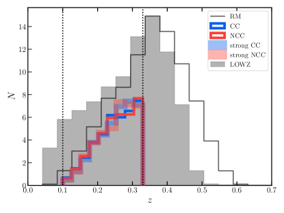
Figure 1: Redshift distribution of the different samples: the full parent cluster sample, redMaPPer (black line), CC and NCC samples (thick blue and red lines, respectively), strong CC and NCC (thin blue and red lines, respectively), and the LOWZ galaxy sample (gray). All samples have arbitrary normalization.

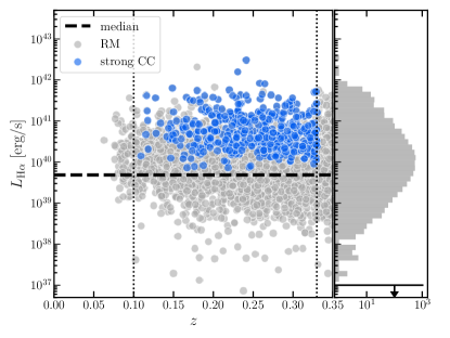
Figure 2: H$\alpha$ luminosity for each redMaPPer BCG with robustly measured spectroscopy as a function of redshift. The redshift limits adopted are marked as vertical dotted lines. Dashed black line indicates the median luminosity threshold above (below) which clusters are considered CC (NCC) clusters. We also mark clusters which are considered strong CC (blue points), for which the H$\alpha$ luminosity detection is significant (i.e., AoN$>2$; see subsubsection 2.1.2). Equivalently, those with no H$\alpha$ emission line detected are considered strong NCC (not marked on this logarithmic scatter plot, but indicated by the black upper limit drawn on the histogram to the right).

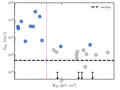
Figure 3: H$\alpha$ luminosity as a function of central entropy inside 20 kpc, $K_{20}$, for each redMaPPer BCG having both spectra from BOSS and entropy measured from the ACCEPT (Chandra) database. Upper limits are drawn for BCGs with no H$\alpha$ emission lines. We mark the median luminosity level (dashed black line) we use to separate CC from NCC, as in Figure 2. The entropy threshold of $K_{20}=60$ keV cm² used in M17 to separate CC and NCC clusters is marked as vertical dotted magenta line. Strong CC clusters are indicated as blue circles. Evidently, all clusters previously considered as CC by the entropy threshold are indeed strong CC clusters using the H$\alpha$ definition.

We use the latest optically selected galaxy cluster catalog detected from SDSS/DR8 with the redMaPPer cluster finder algorithm version 6.3 (Rykoff et al., 2014, 2016) available online. For each cluster, the catalog lists redshift, richness estimate $\lambda$ (approximately the number of cluster galaxies above $0.2\,L_{*}$) and a position, where the position is that of the BCG. BCG identification in redMaPPer is good to 85% (Rykoff et al., 2014; Rozo & Rykoff, 2014; Hoshino et al., 2015). This version of the catalog contains a total of 26,111 clusters detected in $\sim 10,000$ deg², spanning redshifts in the range $0.08<z<0.6$ and richnesses $\lambda>20$. We present the redshift distribution of the full cluster sample in Figure 1 (black), where throughout we use the spectroscopic redshift from SDSS (see item 3 in subsubsection 2.1.1). A cluster random catalog1 has also been constructed (Rykoff et al., 2016), appropriate for large-scale two-point correlation studies such as the one conducted here. We use weights provides in the random catalog to account for survey depth and redshift completeness. Since we aim to cross-correlate the clusters with the LOWZ galaxy catalog, both catalogs need to span the same spatial region on the sky. For LOWZ, some patches observed early on in the survey were masked due to a bug in the initial targeting software (see Reid et al., 2016). We therefore apply the LOWZ North and South masks onto the redMaPPer cluster and random catalog. Finally, we confine our analysis to clusters within $0.1<z<0.33$ for an approximately volume-limited sample (Miyatake et al., 2016), and apply the same redshift limits to the random sample.

2.1.1 Emission-line luminosity as a cool-core indicator

In order to determine if a cluster is in CC or NCC phase, we search for signatures of cooling in the spectrum of its BCG. It has been shown that clusters that harbor multiphase gas with a cool gas core and low central entropy ($\lesssim 30$ keV cm²) typically also exhibit strong emission-line luminosities from H$\alpha$ filaments of gas cooling onto their BCG (e.g., Cavagnolo et al., 2008; McDonald, 2011; Gaspari et al., 2018). We therefore calculate H$\alpha$ emission-line luminosities for each redMaPPer BCG following these steps:

1. We query emission-line fluxes from the emissionLinesPort table (Thomas et al., 2013) in SDSS/DR12 for all galaxies within the same redshift range as the clusters.

2. Where there are duplicate spectra per galaxy (i.e., measured by both SDSS and BOSS), we use the most recent one (BOSS).

3. We cross-match the redMaPPer catalog with the emission line table using the SDSS objid identifier. This provides emission line flux estimates (and spectroscopic redshift) for each cluster. About 17,000 (out of the 26,000) are left after this matching.

4. We remove entries where no H$\alpha$ continuum was measured (i.e., Flux_Cont_Ha_6562=$-9999$ or Flux_Cont_Ha_6562_Err=0) or measured with low signal-to-noise, S/N$<5$.

5. We convert flux to luminosity using the base cosmology and the BCG spectroscopic redshift.

6. For low redshift galaxies ($z<0.3$), the aperture size of the spectral fiber can be smaller than the galaxy size, causing the luminosity to be underestimated. Following McDonald (2011), we correct for this effect by assuming no redshift evolution of the emission-line luminosity, and fit a power-law model to $L(z)$. Since the fiber size changed from $3\arcsec$ in the SDSS phase to $2\arcsec$ in the BOSS phase, we calculate the correction separately for SDSS and BOSS spectra (determined by plate number).

In total, we are left with 6,687 clusters with emission-line information on their BCG in the redshift range $0.1<z<0.33$ with LOWZ spatial coverage. The main limiting factor is the redshift range we adopt.

We present the corrected H$\alpha$ luminosity as a function of redshift in Figure 2 for all the BCGs in the redMaPPer sample. Many ($\sim 30\%$) BCGs have emission-line luminosities below the tail of the distribution, $L_{\mbox{H$\alpha$}}\lesssim 10^{38}$ erg/s, with nearly all having no H$\alpha$ detection (indicted as an upper limit on the histogram).

Next, we examine the correlation of emission-line luminosity with central entropy. We use the ACCEPT sample by Cavagnolo et al. (2009) who measured entropy profiles for 241 clusters observed with Chandra. We cross-match between redMaPPer and the ACCEPT catalog within a $0.5\arcmin$ aperture, resulting in 30 clusters. In Figure 3 we plot the H$\alpha$ emission-line luminosity as a function of central entropy, $K_{20}$, defined as the mean entropy inside 20 kpc. Clusters with no H$\alpha$ detection (i.e., Flux_Ha_6562=0) are indicated as upper limits (arbitrary-level barred arrows; no errorbars are given for these null measurements). As can be seen from the figure, the luminosities are anti-correlated with the central entropy, as previously reported. Specifically, below $K_{20}=60$ keV cm^-2 (pink dotted vertical line), the threshold we have used in M17 to separate CC from NCC, all clusters have significantly higher luminosities, indicative of stronger cooling flows onto their BCG.

2.1.2 CC and NCC sample definitions

We now use the H$\alpha$ luminosity information to create CC and NCC subsamples from the parent redMaPPer sample. First, we divide the sample evenly by the median luminosity value indicated by the dashed black line in both Figure 2 and Figure 3. All clusters above this value are considered CC, while those below are considered NCC. However, selecting CCs based on H$\alpha$ lines introduced a bias, since such features can be better determined at lower redshifts. This makes the redshift distribution of CCs skewed toward lower redshift with respect to that of NCCs. For this reason, we match the redshift distributions of the CC and NCC samples by downsampling both samples. This reduced the sample sizes further by $\sim 10\%$ to about 3,000 clusters in each. The redshift distributions of CC (blue) and NCC (red) subsamples after this procedure are presented in Figure 1. Their mean redshift is $\langle z\rangle=0.25\pm 0.06$.

As noted in the emissionLinePort documentation, some fits to the spectra do not yield significant emission-line flux measurements. Only those with amplitude-over-noise (AoN) larger than two are considered significant emission-line fluxes. We therefore select another more restrictive subset, “strong CC”, of clusters with significant H$\alpha$ flux (AoN_Ha_6562$>2$) totaling 485 clusters. The strong CC sample is presented in Figure 2 and in Figure 3 (matched with ACCEPT) as blue circles. As can be seen from Figure 3, all 9 clusters below our previous entropy-based definition ($K_{20}<60$ keV cm²) are considered strong CC based on the new H$\alpha$ definition, and only two strong CC clusters are considered NCC based on their entropy. Raising the AoN threshold further to exclude those would cut the strong CC sample in half ($\sim$280 clusters), too small for a statistically significant analysis. The

We similarly select a restrictive “strong NCC” subset of clusters with no H$\alpha$ line detection (i.e., Flux_Ha_6562=0), totaling 1,778 clusters6. The redshift distributions of the strong CC and NCC6 are also indicated in Figure 1 as thick transparent blue and red lines, respectively. Their mean redshifts are the same as for their parent CC/NCC samples. We summarize the basic properties of all the cluster subsamples in Table 1.

One limitation of the redMaPPer algorithm is that it a-priori selects “red” galaxies as cluster members. For this reason, strong CC clusters with extreme star-formation in their BCGs leading to bluer colors may be missing from this catalog. Rykoff et al. (2014) show examples of known CC clusters that are still detected, but their BCG is misidentified, leading to larger miscentering. In our above classification, such misidentification may lead to assignment of a CC cluster as NCC. However, Rykoff et al. (2014) demonstrate that such catastrophic miscentering happens for roughly $\lesssim 5\%$ of all clusters. We therefore do not expect a large contamination of the NCC sample by CCs. However, as also indicated from the final sizes of our strong CC/NCC samples, this selection effect does diminish the number of strong CCs in the catalog.

2.1.3 Richness as a mass proxy

The bias of halos on galaxy cluster scales depends first and foremost on mass. Thus, it is important to ensure that the two cluster subsamples we compare have comparable mean mass before exploring any secondary dependencies on other properties. The redMaPPer  catalog contains a richness measurement for each cluster, which can be considered as a mass proxy. Although richness is a very noisy mass proxy, our samples are large enough that the error on the mean mass of each sample is small. In the Appendix A, we will explore the level of uncertainty in the use of richness as a mass proxy by randomly subsampling from the redMaPPer sample. We present the richness distribution for the CC, NCC, strong CC and strong NCC samples in Figure 4. The samples have consistent distributions, and their mean richness (and therefore, mass) are consistent within the errors. We list the mean mass based on the mass-richness relation from (Simet et al., 2017) in Table 1.

We will further explore the mean masses of each cluster subsample using weak gravitational lensing in subsection 4.1.

Table 1: Galaxy and Cluster Samples Properties

Name	$N$	$\log\langle L_{\mbox{H$\alpha$}}\rangle$	${M^{\lambda}_{200\rm m}}$	$M^{\rm lens}_{\rm 200m}$
		[ergs/s]	$\times 10^{14}\,h^{-1}\,M_{\sun}$	$\times 10^{14}\,h^{-1}\,M_{\sun}$
LOWZ	239904
redMaPPer	6687
CC	3053	40.5	1.88$\pm$0.03	$1.99^{+0.21}_{-0.19}$
NCC	3035	39.0	1.90$\pm$0.03	$2.10^{+0.18}_{-0.16}$
strong CC	485	41.0	1.83$\pm$0.07	$1.99^{+0.45}_{-0.40}$
strong NCC	1778	—	1.91$\pm$0.04	$2.11^{+0.23}_{-0.21}$

Note. — Strong NCC are defined as clusters whose BCG has no H$\alpha$ emission line detection, therefore no luminosity is indicated.

2.2 LOWZ galaxy sample

We use the LOWZ spectroscopic-redshift galaxy catalog (Reid et al., 2016), which is drawn from the Baryon Oscillation Spectroscopic Survey (BOSS; Dawson et al., 2013). BOSS is part of SDSS DR12 (Alam et al., 2015). BOSS covers a total effective area of 8,337 deg², and the LOWZ sample contains 463,044 galaxies with spectroscopic redshifts (Reid et al., 2016). We limit both the galaxy catalog and the corresponding random catalog to the redshift range set by the redMaPPer catalog, $0.1<z<0.33$. The basic properties of the cluster and galaxy samples we use in the cross-correlation analysis are listed in Table 1.

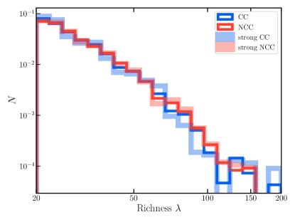
Figure 4: Normalized richness distribution of the different CC and NCC samples, as indicated in the legend.

3 Methods

In this section we detail the two independent methodologies we use for determining the level of assembly bias: clustering and weak lensing.

3.1 Galaxy Clustering

Here we review the methodology developed in M17, cross-correlating a cluster sample with a larger galaxy sample in order to improve the statistical inference. The full details are given in M17, and so we only briefly summarize here.

The simple linear, deterministic galaxy bias relates between the galaxy overdensity, $\delta_{\mathrm{g}}(x)$, and underlying matter overdensity, $\delta(x)$ (Kaiser, 1984),

$$\delta_{\mathrm{g}}(x)=b_{\mathrm{g}}\delta(x)$$ (1)

where overdensity is defined with respect to the mean density, $\delta(x)\equiv\rho(x)/\bar{\rho}-1$. In practice, we make use of the two-point correlation function, $\xi(r)\equiv\langle\delta(x)\delta(x-r)\rangle$ (Peebles, 1973, 1980). Under the above assumptions, the galaxy bias relates the galaxy two-point auto-correlation to the underlying matter correlation function, such that,

$$\xi_{\rm g}(r)=b_{\mathrm{g}}^{2}\xi_{\rm m}(r).$$ (2)

Spectroscopic observations of galaxies typically allow us to measure the galaxy correlation function. In the linear, deterministic galaxy bias model, it is proportional to the correlation function of the underlying matter distribution, described by a constant factor.

One can alternatively cross-correlate different samples of galaxies, or galaxies and clusters as in our case. For the galaxy-cluster CCF, the above model yields

$$\mbox{$\xi_{\rm g,cl}$}(r)=b_{\rm g}b_{\rm cl}\xi_{\rm m}(r)\,,$$ (3)

where $b_{\rm g}$ and $b_{\rm cl}$ denote the galaxy and the cluster bias, respectively. Since we correlate each of the two cluster samples (CC, NCC) with the same galaxy sample (LOWZ in our case), the ratio of these two cross-correlations simply traces the relative bias of NCC clusters with respect to CC clusters,

$$\mbox{$\mbox{$\mathcal{b}$}^{\rm(cross)}$}(r)\equiv b_{\rm NCC}/b_{\rm CC}=\frac{\xi_{\rm g,NCC}(r)}{\xi_{\rm g,CC}(r)}\,.$$ (4)

The galaxy bias term, $b_{\textrm{g}}$, automatically cancels out. Note that using clustering alone (without assuming a halo model) one cannot constrain the individual cluster biases, $b_{\rm CC},~{}b_{\rm NCC}$, without assuming a cosmological model. We can instead constrain their ratio, the relative bias, defined as $\mathcal{b}$, and the superscript notation (cross) indicates the use of CCFs in the measurement.

Similarly, the ACF of clusters, $\xi_{\rm cl}(r)$, would simply be

$$\mbox{$\xi_{\rm cl}$}(r)=b_{\rm cl}^{2}\xi_{\rm m}(r),$$ (5)

so that the relative bias can be derived from the CC and NCC auto-correlations as,

$$\mbox{$\mbox{$\mathcal{b}$}^{\rm(auto)}$}(r)=\sqrt{\frac{\xi_{\rm NCC}(r)}{\xi_{\rm CC}(r)}.}$$ (6)

The disadvantage of the ACF is that it is measured with a lower statistical precision compared to the CCF, since it requires the use of the smaller cluster sample.

3.2 Weak Lensing

Weak gravitational lensing (WL) induces a coherent tangential distortion to the shapes of background galaxies, proportional to the underlying halo excess surface mass density profile of the lensing cluster. The WL signal is related to the cluster-matter cross-correlation function and therefore allows us to determine both the halo total mass (to validate the CC/NCC samples have similar masses), and also independently infer the linear bias parameter from the larger scales of the lensing profile.

The WL methodology as applied to SDSS has been extensively reviewed in the literature (e.g., Mandelbaum et al., 2005, 2013; Simet et al., 2017; Murata et al., 2018), so we only briefly summarize it here. We estimate the mean projected cluster mass density excess profile $\mbox{$\Delta\Sigma$}(r)$ by stacking the shear (as measured from the ellipticities) of source galaxies $s$ over multiple clusters $l$ that lie within a given cluster-centric radial annulus $r$,

$$\mbox{$\Delta\Sigma$}(r)=B(r)\frac{1}{2\mathcal{R}}\frac{\sum\limits_{l,s}w_{ls}e_{t,ls}\mbox{$\Sigma_{\rm cr}$}_{,ls}}{\sum\limits_{l,s}w_{ls}},$$ (7)

where the double summation is over all clusters and over all sources associated with each cluster (i.e., lens-source pairs). $\mbox{$\Sigma_{\rm cr}$}=\frac{c^{2}}{4\pi G}\frac{D_{A}(z_{s})}{D_{A}(z_{l})D_{A}(z_{l},z_{s})(1+z_{l})^{2}},$ is the critical surface mass density, where $G$ is the gravitational constant, $c$ is the speed of light, $z_{l}$ and $z_{s}$ are the lens and source redshifts, respectively, and $D_{A}(z_{l})$, $D_{A}(z_{s})$, and $D_{A}(z_{l},z_{s})$ are the angular diameter distances to the lens, the source, and the lens-to-source, respectively. The extra factor of $(1+z_{l})^{2}$ comes from our use of comoving coordinates (Bartelmann & Schneider, 2001). The photometric redshifts of source galaxies were estimated with zebra and a photometric redshift bias correction was applied (Nakajima et al., 2012). The minimum variance estimator requires the weights to be $w_{ls}=\frac{1}{\mbox{$\Sigma_{\rm cr}$}_{,ls}^{2}}\frac{1}{\sigma_{e,s}^{2}+e_{{\rm rms}}^{2}}$, where $\sigma_{e}$ is the shape measurement uncertainty due to pixel noise, and $e_{\rm rms}=0.365$ is the intrinsic shape noise. The ‘shear responsivity’ factor, ${2\mathcal{R}}$, represents the response of the ellipticity, $e$, to a small shear (Kaiser, 1995; Bernstein & Jarvis, 2002). The factor $B(r)$, corresponds for the boost factor, needed to correct for the dilution effect, which arises from contamination by unlensed cluster galaxies having imperfect photometric redshift estimates. The boost is estimated by comparing the weighted number density of source-lens pairs to that around randoms points, $B(r)=\frac{N_{r}}{N_{l}}\frac{\sum_{ls}w_{ls}}{\sum_{rs}w_{rs}}$.

Following Miyatake et al. (2016), we fit each lensing profile with a five-parameter model,

$$\begin{split}\Delta\Sigma&(r;\mbox{$M_{\mathrm{\rm 200m}}$},c_{200\rm m},q_{\rm cen},\alpha_{\rm off},b)=\\ &q_{\rm cen}\Delta\Sigma^{\rm NFW}(r;\mbox{$M_{\mathrm{\rm 200m}}$},c_{200\rm m})\\ &+(1-q_{\rm cen})\Delta\Sigma^{\rm NFW,off}(r;\mbox{$M_{\mathrm{\rm 200m}}$},c_{200\rm m},\alpha_{\rm off})\\ &+\Delta\Sigma^{\rm 2-halo}(r;b).\end{split}$$ (8)

The first term arises from the halo mass profile for a fraction $q_{\rm cen}$ of clusters whose BCGs as identified by redMaPPer represent the true cluster centers, while the second term describes the profile of the off-centered clusters. We assume that the offsets follow a Gaussian distribution in three dimensions, with $u_{\rm off}\propto\exp{\left[-r^{2}/(2\alpha_{\rm off}^{2}r_{200\rm m}^{2})\right]}$, where $\alpha_{\rm off}$ describes the ratio of the off-centering radius to $r_{200\rm m}$, the radius at which the enclosed mass density is 200 times the mean density of the universe. For both components we adopt the smoothly-truncated NFW (Navarro, Frenk, & White, 1996) model (Oguri & Hamana, 2011). The final term models the contribution from the surrounding large-scale structure, i.e., the two-halo term. We employ the model given as $\Delta\Sigma^{\rm 2-halo}(r;b)=b\int{k{\rm d}k/(2\pi)\bar{\rho}_{m}P^{\rm L}_{\rm m}(k;z_{\rm cl})J_{2}(kr)}$, where $\bar{\rho}_{m}$ is the mean mass density today, $b$ is the linear bias parameter, and $P^{\rm L}_{\rm m}(k;z_{\rm cl})$ is the linear mass power spectrum at the averaged cluster redshift $z_{\rm cl}=0.25$, for the $\Lambda$CDM model. We can then directly probe the relative bias from the individual bias parameters fitted to the lensing profile, defined as

$$\mbox{$\mbox{$\mathcal{b}$}^{\rm 2h}$}\equiv\frac{b_{\rm NCC}}{b_{\rm CC}}.$$ (9)

As a baseline expectation, we can use the halo bias model of (Tinker et al., 2010), calibrated from numerical simulations, in order to estimate the expected halo bias level for each sample based on the derived mean WL mass. Under the zeroth order assumption of no assembly bias, we can then define the expected relative bias as,

$$\mbox{$\mbox{$\mathcal{b}$}^{\rm 0}$}\equiv\frac{b(M_{\rm NCC})}{b(M_{\rm CC})}.$$ (10)

Any deviation from this value should therefore give an estimate of the level of assembly bias. Specifically, we define $f$ as the ratio of the measured bias from each methodology defined above (e.g., $\mbox{$\mathcal{b}$}^{\rm(cross)}$, $\mbox{$\mathcal{b}$}^{\rm(auto)}$, $\mbox{$\mathcal{b}$}^{\rm 2h}$) to the expected mass-only bias, $\mbox{$\mathcal{b}$}^{\rm 0}$, such that our model for the measured bias is

$$\mbox{$\mathcal{b}$}=f\mbox{$\mbox{$\mathcal{b}$}^{\rm 0}$}.$$ (11)

Confirmation of assembly bias requires $f\neq 1$. We will therefore obtain the marginalized posterior distribution of $f$ from fitting the above model to each measured relative bias. We perform the fitting with the public code emcee (Foreman-Mackey et al., 2013).

4 Results

In this section we present the WL and clustering analyses of the CC and NCC cluster samples defined above and the mean relative bias we derive for each methodology.

4.1 Weak Lensing

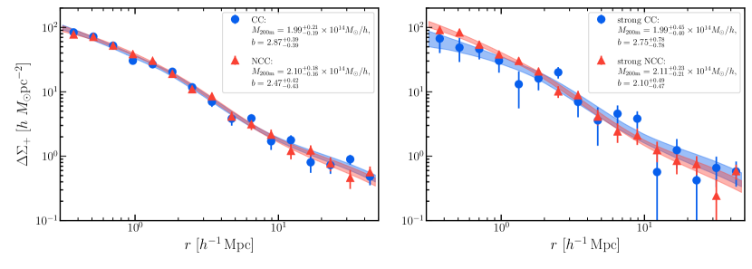
Figure 5: Stacked cluster WL excess surface mass density profiles for the CC and NCC samples (left), and the strong CC/NCC samples (right). Mean masses and halo bias values derived from model fitting the WL profiles are given next to each set. The NCC mean mass is about $1\sigma$ above the CC mass (see Table 1), whereas the CC galaxy bias is about $1\sigma$ above the NCC galaxy bias (and similarly for the strong CC/strong NCC samples).

Here we make use of lensing data to first determine the mean masses of the CC and NCC cluster samples and test if they are indeed comparable as indicated by the mass-richness scaling relation. Subsequently, cluster WL profiles will be used to determine the level of expected mass bias and the level of measured bias.

We use the SDSS/DR8 shape catalog (Reyes et al., 2012; Mandelbaum et al., 2013) measured with the reGaussianization technique (Hirata & Seljak, 2003). The systematic uncertainties on shape measurements have been thoroughly investigated in Mandelbaum et al. (2005). We measure the stacked WL excess surface mass density profile, $\Delta\Sigma(r)$ (Equation 7), in 16 logarithmically-spaced radial bins in the range 0.3–50 $h^{-1}\,\mathrm{Mpc}$. We present the resulting profiles in Figure 5 for both the CC/NCC (left, circles and triangles, respectively) and the strong CC/NCC (right) samples. The covariance is derived using the jackknife method, dividing the sample into 83 equal area bins. The figure demonstrates that the two subsamples have very similar mass profiles.

We fit for both the one- and two-halo terms simultaneously, setting flat priors on the mass, $M_{\mathrm{\rm 200m}}$, concentration, $c_{\rm 200m}$, and halo bias $b$. We set restrictive gaussian priors on the miscentering parameters, around the nominal values presented in Simet et al. (2017). We do this since the profiles are not well constrained at the center, $r<300$ kpc, and miscentering is highly degenerate with the concentration parameter. For the same reason, we do not fit for a central stellar mass contribution from the BCG. The fitted masses are listed for each cluster sample in Table 1. We find overall consistent masses for the CC/NCC samples, $M_{\rm CC}=1.99^{+0.21}_{-0.19}\mbox{$\times 10^{14}\,h^{-1}\,M_{\sun}$}$, and $M_{\rm NCC}=2.10^{+0.18}_{-0.16}\mbox{$\times 10^{14}\,h^{-1}\,M_{\sun}$}$. The strong CC/NCC also show similarly consistent masses, $M_{\rm stCC}=1.99^{+0.45}_{-0.40}\mbox{$\times 10^{14}\,h^{-1}\,M_{\sun}$}$, and $M_{\rm stNCC}=2.11^{+0.23}_{-0.21}\mbox{$\times 10^{14}\,h^{-1}\,M_{\sun}$}$. For both cases, mean masses are consistent within 1$\sigma$.

As presented in subsection 3.2, we can calculate the expected mass-only bias (Equation 10). Using the Tinker et al. (2010) halo bias model provided in the python colossus toolkit (Diemer, 2018), we translate each lensing mass in the MCMC chains to bias. We then derive the relative bias by dividing each of NCC bias values with each of the CC bias values. The expected bias ratio of CC and NCC clusters is $\mbox{$\mbox{$\mathcal{b}$}^{\rm 0}$}=1.05^{+0.07}_{-0.06}$. For the strong CC and strong NCC samples, the expected relative bias is $\mbox{$\mbox{$\mathcal{b}$}^{\rm 0}$}=1.05^{+0.13}_{-0.11}$. Therefore, based on the masses, the LSS around NCC is not expected to be significantly more clustered than around CC clusters ($\lesssim 5\%$). These results are summarized in the first row of Table 2.

In comparison, the linear biases directly estimated from the two-halo fit show a ratio that is statistically consistent with that expected from the lensing masses, though the central value is about $1\sigma$ below. In the case of CC/NCC, we measure $b_{\rm CC}=2.87\pm{0.39}$, and $b_{\rm NCC}=2.47^{+0.42}_{-0.43}$. As defined in Equation 9, this translates to a relative bias of $\mbox{$\mbox{$\mathcal{b}$}^{\rm 2h}$}=0.86\pm{0.20}$. For the strong CC/NCC samples, we find $b_{\rm stCC}=2.75\pm{0.78}$, and $b_{\rm stNCC}=2.10^{+0.49}_{-0.47}$, i.e., a relative bias of $\mbox{$\mbox{$\mathcal{b}$}^{\rm 2h}$}=0.89^{+0.67}_{-0.54}$. The two-halo bias results are summarized in the second row of Table 2. We will quantify the significance and interpretation of these different results in subsection 5.1, together with the two-point clustering results presented next.

Table 2: Results of the bias analysis from different methodologies

	CC/NCC		Strong CC/NCC
Method	$\mathcal{b}$	$f$	$\mathcal{b}$	$f$
Lensing
1-halo (expected)	$1.05_{-0.06}^{+0.07}$	$1$	$1.05_{-0.11}^{+0.13}$	$1$
2-halo	$0.86_{-0.20}^{+0.20}$	$0.83_{-0.20}^{+0.20}$	$0.89_{-0.54}^{+0.67}$	$0.86_{-0.52}^{+0.66}$
Clustering
$\xi_{\rm g,cl}$	$1.01_{-0.03}^{+0.03}$	$0.97_{-0.06}^{+0.07}$	$0.98_{-0.06}^{+0.06}$	$0.94_{-0.11}^{+0.13}$
$\xi_{\rm g,cl}$, projected	$0.97_{-0.06}^{+0.06}$	$0.93_{-0.08}^{+0.08}$	$0.82_{-0.10}^{+0.10}$	$0.79_{-0.12}^{+0.13}$
$\xi_{\rm cl}$	$1.02_{-0.06}^{+0.06}$	$0.98_{-0.08}^{+0.08}$	$0.97_{-0.22}^{+0.22}$	$0.93_{-0.23}^{+0.25}$

Note. — $\mbox{$\mathcal{b}$}=b_{\mathrm{NCC}}/b_{\mathrm{CC}}$ measures the level of relative bias between the NCC and CC clusters. $f=\mbox{$\mathcal{b}$}/\mbox{$\mbox{$\mathcal{b}$}^{\rm 0}$}$ measures the level of assembly bias. Median and 68% confidence bounds are quoted.

4.2 Clustering

Figure 6: Each upper panel in the plots shows the real-space two-point correlation functions for the CC (blue) and and NCC (red), while the bottom panels show the relative bias (black) derived from the ratio of the CC/NCC correlation functions above it, as a function of comoving separation, $r$. Left plots show the results for the median-divided CC/NCC samples, whereas right plots show the strong CC/NCC samples (see Table 1 for definitions). Top and bottom plots use different clustering methodologies. Top: using the CCFs between galaxies and clusters, $\xi_{\rm g,cl}$(r). Bottom: using the ACFs of the cluster samples, $\xi_{\rm cl}$(r). Overall, the results are consistent between the different methodologies. The CCF methodology, however, yields tighter constraints than the ACF due to the larger galaxy sample employed.

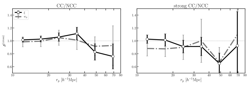
Figure 7: Relative bias from cross-correlation as a function of separation, but calculated using the projected CCF, $w_{\rm p}(r_{\rm p})$ (gray dash-dotted line). The signal is consistent with that derived from the real-space CCF (black, same as the black solid lines in the top plots of Figure 6).

Here we measure the relative bias from the clustering profiles on large-scales using the two-point correlation functions as defined in section 3. We make use of the public code corrfunc (Sinha & Garrison, 2017), which relies on the Landy & Szalay (1993) estimator, to calculate all the two-point correlation functions. We first compute the CCF of each cluster subsample (CC, NCC, strong CC and strong NCC) with the LOWZ galaxies. In order to avoid redshift-space distortions that affect galaxies infalling into halos, we need to compute the CCF outside the cluster one-halo regime. We evaluate this scale by computing the velocity dispersion of each cluster subsample from the peculiar velocities of LOWZ galaxies inside 1.5 $h^{-1}\,\mathrm{Mpc}$ of a nearby cluster halo. The CC and NCC samples show $\Delta V\simeq 700$ km/s, corresponding roughly to a virial radius of 1 $h^{-1}\,\mathrm{Mpc}$. We furthermore compute the two-dimensional CCF as a function of projected ($r_{p}$) and line-of sight ($\pi$) distance, $\xi(r_{p},\pi$). Finger-of-god effects are evident up to scales $\lesssim 10$ $h^{-1}\,\mathrm{Mpc}$. We therefore choose to compute the real space CCF (Equation 3) in six logarithmic bins in the range 10–80 $h^{-1}\,\mathrm{Mpc}$. Throughout, the full covariance matrix is derived using the jackknife method for each of the correlation functions and the bias profiles, by diving the SDSS/redMaPPer area into 192 equal area regions. The results are presented in the top panels of Figure 6. The upper panel of the left plot shows the CCFs, $\mbox{$\xi_{\rm g,cl}$}(r)$, of the CC (blue) and NCC (red) clusters, and the bottom panel shows the bias, $\mbox{$\mbox{$\mathcal{b}$}^{\rm(cross)}$}(r)$ (black), derived from the ratio of the two CCFs (Equation 4). The right panel shows the same for the strong CC and strong NCC cluster subsamples. To estimate the mean bias level we fit $\mbox{$\mathcal{b}$}(r)$ with a constant model taking into account the covariance between scales. The median relative bias, $\mbox{$\mathcal{b}$}^{\rm(cross)}$, and its uncertainty, are summarized in Table 2. Apparently, there is no significant difference between the clustering around CC versus NCC, $\mbox{$\mbox{$\mathcal{b}$}^{\rm(cross)}$}=1.01\pm 0.03$. The bias for strong CC/NCC is also non-significant, $\mbox{$\mbox{$\mathcal{b}$}^{\rm(cross)}$}=0.98\pm 0.06$.

Another common methodology is to calculate the ACF of the clusters themselves, $\xi_{\rm cl}(r)$, given by Equation 5, where the relative bias equals the square-root of the ratio of the ACFs (Equation 6). Naturally, this methodology yields larger errors, but may serve as a semi-independent check of the bias, since the LOWZ galaxy sample is not included here. We present the results for the CC/NCC and strong CC/NCC samples in the bottom plots of Figure 6. The ACF also show a bias fully consistent with the expected level, $\mbox{$\mbox{$\mathcal{b}$}^{\rm(auto)}$}=1.02\pm 0.06$ for the CC/NCC, and $\mbox{$\mbox{$\mathcal{b}$}^{\rm(auto)}$}=0.97\pm 0.22$ for the strong CC/NCC. The results are summarized in the last row of Table 2. We will compare the clustering results with those derived from lensing and interpret them in the context of assembly bias in subsection 5.1.

Lastly, to validate that the real-space CCF are not affected by residual redshift-space distortions (RSD) effects, we also compute the projected CCF, $\mbox{$w_{\rm p}$}(r_{\rm p})$, integrated along the line of sight to $\pi=100$ $h^{-1}\,\mathrm{Mpc}$. Such integration removes any issues due to RSD. The results, shown as dashed lines in Figure 7, are consistent with those derived from the real-space CCF, $\mbox{$\xi_{\rm g,cl}$}(r)$.

5 Discussion

5.1 Significance of Assembly Bias

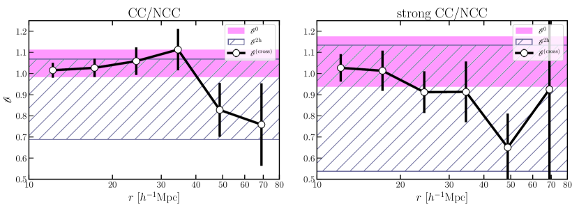
Figure 8: Comparison of the relative bias measured with cross-correlation, $\mbox{$\mathcal{b}$}^{\rm(cross)}$$(r)$ (black points, same as in top panels of Figure 6) and with lensing, $\mbox{$\mathcal{b}$}^{\rm 2h}$(68% confidence region; hatched). These two are compared with the level of expected mass-only relative bias $\mbox{$\mathcal{b}$}^{\rm 0}$(68% confidence region; pink), calculated using the Tinker et al. (2010) halo bias model with the WL-derived masses as input. The two measurements are consistent within $\lesssim 1\sigma$ with the expected mass-only bias level, for both the CC/NCC and strong CC/NCC samples, i.e., showing no evidence for assembly bias between CC and NCC.

We now explore the level of assembly bias derived from each methodology by comparing it with the expected mass-only bias level, $\mbox{$\mathcal{b}$}^{\rm 0}$, derived from the fitted lensing masses. To visualize these, in Figure 8 we plot the fiducial bias profile measured from the ratio of CCFs, $\mbox{$\mathcal{b}$}^{\rm(cross)}$ (black; same as solid black line in Figure 6). We overlay the lensing-measured relative bias using the fitted bias parameters, $\mbox{$\mathcal{b}$}^{\rm 2h}$ (hatched, 68% confidence region), and finally the expected mass-only bias derived by assuming a Tinker et al. (2010) halo bias model with the WL mean masses as input, $\mbox{$\mathcal{b}$}^{\rm 0}$ (pink, 68% confidence region). It appears that $\mbox{$\mathcal{b}$}^{\rm(cross)}$agrees well with the level derived from the lensing two-halo term, $\mbox{$\mathcal{b}$}^{\rm 2h}$, though the constraints on the latter are poor ($\sim 20-60\%$ confidence level). On the other hand, both measured biases, $\mbox{$\mathcal{b}$}^{\rm(cross)}$ and $\mbox{$\mathcal{b}$}^{\rm 2h}$, are about 1$\sigma$ below the expected level, $\mbox{$\mathcal{b}$}^{\rm 0}$.

To better quantify if the measured bias significantly differs from the expected mass-only bias $\mbox{$\mathcal{b}$}^{\rm 0}$, we fit each measured dataset ($\mbox{$\mathcal{b}$}^{\rm 2h}$, $\mbox{$\mathcal{b}$}^{\rm(cross)}$(r), projected $\mbox{$\mbox{$\mathcal{b}$}^{\rm(cross)}$}(r_{\rm p})$ and $\mbox{$\mbox{$\mathcal{b}$}^{\rm(auto)}$}(r)$) with the model described in Equation 11. For all the clustering results, which were determined as a function of scale, we take into account the full covariance matrix in our likelihood function. Since our parameter of interest is $f$, we set a flat (uninformative) prior on $f$. We set a tight lognormal prior on $\mbox{$\mathcal{b}$}^{\rm 0}$ dictated by the median and standard deviation of $\log(\mbox{$\mbox{$\mathcal{b}$}^{\rm 0}$})$ and then marginalize over it. The posterior values for $f$ are given in Table 2 next to each measured $\mathcal{b}$.

As can be seen, all values of $f$ are consistent with the null hypothesis, $f=1$, up to 1–2$\sigma$. The projected $\mbox{$\mathcal{b}$}^{\rm(cross)}$ measured for the strong CC/NCC samples shows the highest offset, $f=0.79\pm 0.12$ but is still below the $2\sigma$ level. We therefore conclude, based on the redMaPPer cluster sample, that we find no indication of different assembly histories for CC and NCC clusters to within 6% uncertainty.

5.2 Comparison with Simulations

In simulations, assembly bias on cluster scales has been shown to exist in practically all definitions of halo age (Chue et al., 2018), although some proxies appear to be noisier than others (Mao et al., 2018). Recently, combining several N-body simulations covering a wider mass range up to $10^{14.5}h^{-1}\,M_{\odot}$, Sato-Polito et al. (2018) find different secondary indicators of assembly histories yield somewhat different results. For example, if separating halos by their age, no assembly bias is detected above $\times 10^{14}\,h^{-1}\,M_{\sun}$. On the other hand, if separating halos by concentration or spin, at the high-mass end, the difference between the upper and lower quartiles can reach up to a factor of 2.

There is no equivalent in cosmological simulations for the physical distinction we are studying, i.e., the cooling phase of the cluster core gas. This is since baryonic effects, especially considering the large range in scales involved, are currently hard to include (although see Rasia et al., 2015; Barnes et al., 2018). Therefore, any statements about the levels found in simulations are not necessary applicable to our study. Nonetheless, we may consider the above range of bias values found in simulations as a guideline to the degree of assembly bias expected in general. With that in mind, it is safe to conclude we find no significant level of assembly bias in our samples.

Given this measurement alone, we may not identify the specific formation model. Whether cores are created early on and left undisturbed, or whether later periodic CC formation and distruption and in play, we find those to be decoupled from the external environment on large scales. One may argue this is not surprising since the cores are embedded in self-similar envelopes (McDonald et al., 2017). It may, in turn, be that even though their large-scale modes appear the same, small-scale fluctuations result in different initial conditions at the halo regime, e.g., NCC may be the result of a lower amplitude fluctuation with higher substructure. It would thus be interesting to compare the small-scale clustering of CC and NCC clusters at low and high redshift.

6 Summary & Conclusions

In this paper we tested the level of assembly bias between different cluster samples, separated by a physically-motivated criteria: the level of cooling in their cores. We differentiate between CC and NCC clusters solely based on the BCG H$\alpha$ luminosity as a cooling indicator. We draw samples of thousands of CC and NCC clusters from the SDSS/DR8 redMaPPer catalog to achieve a statistically significant measurement of the weak assembly bias effect. We performed a weak lensing analysis measuring the cluster density profiles to investigate their mean mass and two-halo linear bias properties. Furthermore, we applied a complementary and novel methodology, cross-correlating the cluster samples of with an even larger sample of hundreds of thousands of galaxies from the LOWZ sample, to gain better statistical precision on the bias. This method provides information on the large-scale environments of clusters who have apparently different characteristics, which in turn provide insight into their formation history.

From WL we found the CC and NCC samples to have comparable mean masses, $\mbox{$M_{\mathrm{\rm 200m}}$}\approx 2\times\mbox{$\times 10^{14}\,h^{-1}\,M_{\sun}$}$. From the mean WL masses, we quantified the expected level of mass-only bias to be $\mbox{$\mbox{$\mathcal{b}$}^{\rm 0}$}=1.05^{+0.07}_{-0.06}$ for the CC/NCC samples, and $\mbox{$\mbox{$\mathcal{b}$}^{\rm 0}$}=1.05^{+0.13}_{-0.11}$ for the strong CC/NCC samples. We then quantified the departure from the null hypothesis with the assembly bias fraction, $f$, and fitted the measured bias to constrain this parameter. From the lensing two-halo measured bias, $\mbox{$\mathcal{b}$}^{\rm 2h}$, we found no indication of assembly bias, with $f=0.83\pm 0.20$ for CC/NCC and $f=0.86^{+0.66}_{-0.52}$ for the strong CC/NCC. Since the size of the error is approximately at or greater than the expected level of the effect, $\sim 20-70\%$, for the current sample size lensing alone lacks statistical constraining power to probe assembly bias.

From the more sensitive CCF methodology, we fit $\mbox{$\mathcal{b}$}^{\rm(cross)}$and found $f=0.97^{+0.07}_{-0.06}$ for the CC/NCC samples and $f=0.94^{+0.13}_{-0.11}$ for the strong CC/NCC samples. We also applied the more traditional ACF methodology using the clusters alone, and found $f=0.98\pm 0.08$ for CC/NCC and $f=0.93^{+0.25}_{-0.23}$ for the strong CC/NCC, though this methodology is statistically weaker, with similar constraining power as of the lensing methodology. Therefore, within $\sim 1\sigma$, both subsets using both methodologies agree with no assembly bias.

It is important to note that although we have expanded our analysis to make use of thousands of clusters compared to dozens in M17, the redMaPPer sample is inherently biased against heavily star-forming cluster cores (Rykoff et al., 2016). Indeed, our strong CC sample is limited to $\sim$500 clusters only. A future study would benefit from a less biased sample, e.g., not relying on a red-sequence finder (e.g., Soares-Santos et al., 2011; Wen et al., 2012), or one that makes use of future multi-narrowband surveys (e.g., SPHEREx; Doré et al. 2016).

We conclude, based on the results presented in this analysis, that any observed differences between CC and NCC clusters are not inherited from different large-scale environments. In turn, the assignment of the cluster cooling phase may result from different small-scale clustering. Combined with the reported mild evolution in CC properties, one possible solution is that the local gas properties in the protocluster core determine the subsequent creation of an AGN feedback loop. Alternatively, local merger activity could create and destroy CC periodically but in a way that mimics constant mean population properties over time.

While our study cannot confirm either proposed picture, studying clusters at the onset of formation, which appears to be as high as $z\sim 2$, can shed direct light on the process of core formation. We are only now at a stage where the evolution of clusters can be studied statistically with large ensembles, both in observations (McDonald et al., 2017, 2018) and in cosmological simulations (Rasia et al., 2015; Barnes et al., 2018). Such large-scale simulations are at the infancy of incorporating complex AGN feedback and feeding physics via subgrid models, and require better physically-motivated (rather than fine-tuned) schemes in order to achieve robustly predictive results for the CC-NCC formation (e.g., Gaspari & Sa̧dowski, 2017). LSST and WFIRST will revolutionize our understanding of cluster formation and evolution, as they will enable us to study the galaxy populations in $z\lesssim 2$ clusters in the thousands instead of the current dozens. CMB-S4 will both detect clusters up to $z\sim 2$ through the redshift-independent SZ effect and inform on the gas properties at the epoch of clusters formation. Our most pressing challenge is matching those promising optical/IR surveys with the complementary high-resolution spectral and X-ray surveys of cluster cores (e.g., Athena; Ettori et al. 2013) that will facilitate better understanding of the initial buildup and the precise impact of baryonic physics on cluster formation.

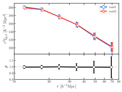
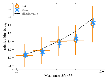
Figure 9: Left: Results from the null test. We randomly select subsamples from the parent redMaPPer catalog and calculate the CCFs and relative bias, clearly validating the null hypothesis: $b=1$ between two random subsamples. Right: Results from the mass bias test. The theoretical relation between relative halo mass bias and the mass ratio is given by the black dashed line, based on Pillepich et al. (2010) simulations. Orange circles and blue crosses show the relative bias in each mass ratio bin measured from simulated MICE clusters and galaxies using the ACF and CCF, respectively. The ACF and CCF methodologies give consistent results, and both are consistent with the expected level.

Appendix A Null test

We perform a null test to validate that our CCF methodology yields no bias ($\mbox{$\mathcal{b}$}=1$) when selecting cluster subsamples randomly. From the parent redMaPPer sample, we select 100 random subsamples each of the same size as our CC/NCC samples ($N=3000$). We preform the same CCF analysis as described in subsection 4.2, cross-correlating each random subsample with the LOWZ catalog. We divide each of the CCFs of the first 50 subsamples (‘rand1’) with each of the last 50 subsamples’ (‘rand2’) CCFs to get $50^{2}$ relaltive bias realizations. The results are presented in the Figure 9 (left). Errors represent the scatter from the random sampling. These errors also take into account both statistical noise and systematics due to the assumption that equal richness distributions represent equal masses. These errors are comparable to the jackknife errors which we use as our fiducial errors.

Appendix B Mass bias test

In this section we test that our CCF methodology retrieves the expected mass bias. For this test, we use the Marenostrum Institut de Cieńcies de l’Espai (MICE) Grand Challenge (MICE-GC) simulations (Fosalba et al., 2015a, b; Crocce et al., 2015; Carretero et al., 2015; Hoffmann et al., 2015), for which the halo mass is known. We define clusters as having $M_{\rm h}>10^{13}M_{\sun}$. We randomly select 20 bootstrap realizations of cluster samples each of size $N=3000$, in each of the six mass bins. We cross-correlate each cluster sample with a mock galaxy sample (selected to mimic the LOWZ sample in terms of color and redshift distribution) over the entire radial range (10 to 80 $h^{-1}\,\mathrm{Mpc}$, as for our data), and divide each of the CCFs of the five highest-mass bins with the CCF of the lowest mass bin. This gives us a test of our CCF methodology: the ratio should give the relative mass bias, $\mbox{$\mathcal{b}$}^{\rm(cross)}$. Since we have 20 mock cluster catalogs in each mass bin, we have overall 400 realizations of the relative bias in each mass ratio bin. We take the scatter as the error on the relative bias. We follow the same exercise for the ACF methodology, measuring $\mbox{$\mathcal{b}$}^{\rm(auto)}$. We plot the expected (black; using the Pillepich et al. (2010) model) and the derived $\mbox{$\mathcal{b}$}^{\rm(cross)}$ (blue crosses) and $\mbox{$\mathcal{b}$}^{\rm(auto)}$ (orange circles) averaged over all scales as a function of mass ratio in Figure 9 (right). As can be seen, the two methodologies are completely consistent with each other. As expected, the CCF methodology yields much smaller uncertainties than ACF. The CCF-derived $\mbox{$\mathcal{b}$}^{\rm(cross)}$ is slightly below the expected values found by Pillepich et al. (2010), but only at high mass ratios (our study is at a mass ratio of $\lesssim 1.2$, as determined in subsection 4.1). We also note that different approaches adopted by different simulation sets may cause this small effect.

References

- Alam et al. (2015) Alam, S., Albareti, F. D., Allende Prieto, C., et al. 2015, ApJS, 219, 12, doi: 10.1088/0067-0049/219/1/12
- Barnes et al. (2018) Barnes, D. J., Vogelsberger, M., Kannan, R., et al. 2018, MNRAS, 481, 1809, doi: 10.1093/mnras/sty2078
- Bartelmann & Schneider (2001) Bartelmann, M., & Schneider, P. 2001, Phys. Rep., 340, 291
- Bernstein & Jarvis (2002) Bernstein, G. M., & Jarvis, M. 2002, AJ, 123, 583, doi: 10.1086/338085
- Busch & White (2017) Busch, P., & White, S. D. M. 2017, MNRAS, 470, 4767, doi: 10.1093/mnras/stx1584
- Carretero et al. (2015) Carretero, J., Castander, F. J., Gaztañaga, E., Crocce, M., & Fosalba, P. 2015, MNRAS, 447, 646, doi: 10.1093/mnras/stu2402
- Cavagnolo et al. (2008) Cavagnolo, K. W., Donahue, M., Voit, G. M., & Sun, M. 2008, ApJ, 682, 821, doi: 10.1086/588630
- Cavagnolo et al. (2009) —. 2009, ApJS, 182, 12, doi: 10.1088/0067-0049/182/1/12
- Chue et al. (2018) Chue, C. Y. R., Dalal, N., & White, M. 2018, J. Cosmology Astropart. Phys, 10, 012, doi: 10.1088/1475-7516/2018/10/012
- Correa et al. (2015) Correa, C. A., Wyithe, J. S. B., Schaye, J., & Duffy, A. R. 2015, MNRAS, 452, 1217, doi: 10.1093/mnras/stv1363
- Crocce et al. (2015) Crocce, M., Castander, F. J., Gaztañaga, E., Fosalba, P., & Carretero, J. 2015, MNRAS, 453, 1513, doi: 10.1093/mnras/stv1708
- Croton et al. (2007) Croton, D. J., Gao, L., & White, S. D. M. 2007, MNRAS, 374, 1303, doi: 10.1111/j.1365-2966.2006.11230.x
- Dawson et al. (2013) Dawson, K. S., Schlegel, D. J., Ahn, C. P., et al. 2013, AJ, 145, 10, doi: 10.1088/0004-6256/145/1/10
- Diemer (2018) Diemer, B. 2018, The Astrophysical Journal Supplement Series, 239, 35, doi: 10.3847/1538-4365/aaee8c
- Donahue et al. (2000) Donahue, M., Mack, J., Voit, G. M., et al. 2000, ApJ, 545, 670, doi: 10.1086/317836
- Doré et al. (2016) Doré, O., Werner, M. W., Ashby, M., et al. 2016, ArXiv e-prints. https://arxiv.org/abs/1606.07039
- Edge (2001) Edge, A. C. 2001, MNRAS, 328, 762, doi: 10.1046/j.1365-8711.2001.04802.x
- Eisenstein et al. (2011) Eisenstein, D. J., Weinberg, D. H., Agol, E., et al. 2011, AJ, 142, 72, doi: 10.1088/0004-6256/142/3/72
- Ettori et al. (2013) Ettori, S., Pratt, G. W., de Plaa, J., et al. 2013, arXiv e-prints. https://arxiv.org/abs/1306.2322
- Fabian (1994) Fabian, A. C. 1994, ARA&A, 32, 277, doi: 10.1146/annurev.aa.32.090194.001425
- Fabian (2012) —. 2012, ARA&A, 50, 455, doi: 10.1146/annurev-astro-081811-125521
- Faltenbacher & White (2010) Faltenbacher, A., & White, S. D. M. 2010, ApJ, 708, 469, doi: 10.1088/0004-637X/708/1/469
- Foreman-Mackey et al. (2013) Foreman-Mackey, D., Hogg, D. W., Lang, D., & Goodman, J. 2013, PASP, 125, 306, doi: 10.1086/670067
- Fosalba et al. (2015a) Fosalba, P., Crocce, M., Gaztañaga, E., & Castander, F. J. 2015a, MNRAS, 448, 2987, doi: 10.1093/mnras/stv138
- Fosalba et al. (2015b) Fosalba, P., Gaztañaga, E., Castander, F. J., & Crocce, M. 2015b, MNRAS, 447, 1319, doi: 10.1093/mnras/stu2464
- Gao et al. (2005) Gao, L., Springel, V., & White, S. D. M. 2005, MNRAS, 363, L66, doi: 10.1111/j.1745-3933.2005.00084.x
- Gao & White (2007) Gao, L., & White, S. D. M. 2007, MNRAS, 377, L5, doi: 10.1111/j.1745-3933.2007.00292.x
- Gaspari (2015) Gaspari, M. 2015, MNRAS, 451, L60, doi: 10.1093/mnrasl/slv067
- Gaspari & Sa̧dowski (2017) Gaspari, M., & Sa̧dowski, A. 2017, ApJ, 837, 149, doi: 10.3847/1538-4357/aa61a3
- Gaspari et al. (2018) Gaspari, M., McDonald, M., Hamer, S. L., et al. 2018, ApJ, 854, 167, doi: 10.3847/1538-4357/aaaa1b
- Ghirardini et al. (2019) Ghirardini, V., Eckert, D., Ettori, S., et al. 2019, A&A, 621, A41, doi: 10.1051/0004-6361/201833325
- Gunn & Gott (1972) Gunn, J. E., & Gott, J. R. I. 1972, ApJ, 176, 1
- Hirata & Seljak (2003) Hirata, C., & Seljak, U. 2003, MNRAS, 343, 459, doi: 10.1046/j.1365-8711.2003.06683.x
- Hlavacek-Larrondo et al. (2015) Hlavacek-Larrondo, J., McDonald, M., Benson, B. A., et al. 2015, ApJ, 805, 35, doi: 10.1088/0004-637X/805/1/35
- Hoffmann et al. (2015) Hoffmann, K., Bel, J., Gaztañaga, E., et al. 2015, MNRAS, 447, 1724, doi: 10.1093/mnras/stu2492
- Hoshino et al. (2015) Hoshino, H., Leauthaud, A., Lackner, C., et al. 2015, MNRAS, 452, 998, doi: 10.1093/mnras/stv1271
- Hudson et al. (2010) Hudson, D. S., Mittal, R., Reiprich, T. H., et al. 2010, A&A, 513, A37, doi: 10.1051/0004-6361/200912377
- Kaiser (1984) Kaiser, N. 1984, ApJ, 284, L9, doi: 10.1086/184341
- Kaiser (1995) —. 1995, ApJ, 439, L1, doi: 10.1086/187730
- Lacerna & Padilla (2012) Lacerna, I., & Padilla, N. 2012, Monthly Notices of the Royal Astronomical Society: Letters, 426, L26, doi: 10.1111/j.1745-3933.2012.01316.x
- Landy & Szalay (1993) Landy, S. D., & Szalay, A. S. 1993, ApJ, 412, 64, doi: 10.1086/172900
- Lazeyras et al. (2017) Lazeyras, T., Musso, M., & Schmidt, F. 2017, J. Cosmology Astropart. Phys, 3, 059, doi: 10.1088/1475-7516/2017/03/059
- Li et al. (2008) Li, Y., Mo, H. J., & Gao, L. 2008, MNRAS, 389, 1419, doi: 10.1111/j.1365-2966.2008.13667.x
- Lin et al. (2016) Lin, Y.-T., Mandelbaum, R., Huang, Y.-H., et al. 2016, ApJ, 819, 119, doi: 10.3847/0004-637X/819/2/119
- Ludlow et al. (2013) Ludlow, A. D., Navarro, J. F., Boylan-Kolchin, M., et al. 2013, MNRAS, 432, 1103, doi: 10.1093/mnras/stt526
- Mandelbaum et al. (2013) Mandelbaum, R., Slosar, A., Baldauf, T., et al. 2013, MNRAS, 432, 1544, doi: 10.1093/mnras/stt572
- Mandelbaum et al. (2005) Mandelbaum, R., Tasitsiomi, A., Seljak, U., Kravtsov, A. V., & Wechsler, R. H. 2005, MNRAS, 362, 1451, doi: 10.1111/j.1365-2966.2005.09417.x
- Mao et al. (2018) Mao, Y.-Y., Zentner, A. R., & Wechsler, R. H. 2018, MNRAS, 474, 5143, doi: 10.1093/mnras/stx3111
- McDonald (2011) McDonald, M. 2011, ApJ, 742, L35, doi: 10.1088/2041-8205/742/2/L35
- McDonald et al. (2018) McDonald, M., Gaspari, M., McNamara, B. R., & Tremblay, G. R. 2018, ApJ, 858, 45, doi: 10.3847/1538-4357/aabace
- McDonald et al. (2010) McDonald, M., Veilleux, S., Rupke, D. S. N., & Mushotzky, R. 2010, ApJ, 721, 1262, doi: 10.1088/0004-637X/721/2/1262
- McDonald et al. (2012) McDonald, M., Wei, L. H., & Veilleux, S. 2012, ApJ, 755, L24, doi: 10.1088/2041-8205/755/2/L24
- McDonald et al. (2017) McDonald, M., Allen, S. W., Bayliss, M., et al. 2017, ApJ, 843, 28, doi: 10.3847/1538-4357/aa7740
- McNamara & Nulsen (2007) McNamara, B. R., & Nulsen, P. E. J. 2007, ARA&A, 45, 117, doi: 10.1146/annurev.astro.45.051806.110625
- McNamara & Nulsen (2012) —. 2012, New Journal of Physics, 14, 055023, doi: 10.1088/1367-2630/14/5/055023
- Medezinski et al. (2017) Medezinski, E., Battaglia, N., Coupon, J., et al. 2017, ApJ, 836, 54, doi: 10.3847/1538-4357/836/1/54
- Miyatake et al. (2016) Miyatake, H., More, S., Takada, M., et al. 2016, Physical Review Letters, 116, 041301, doi: 10.1103/PhysRevLett.116.041301
- Montero-Dorta et al. (2017) Montero-Dorta, A., Pérez, E., Prada, F., et al. 2017, Astrophysical Journal Letters, 848, doi: 10.3847/2041-8213/aa8cc5
- More et al. (2016) More, S., Miyatake, H., Takada, M., et al. 2016, ApJ, 825, 39, doi: 10.3847/0004-637X/825/1/39
- Murata et al. (2018) Murata, R., Nishimichi, T., Takada, M., et al. 2018, ApJ, 854, 120, doi: 10.3847/1538-4357/aaaab8
- Nakajima et al. (2012) Nakajima, R., Mandelbaum, R., Seljak, U., et al. 2012, MNRAS, 420, 3240, doi: 10.1111/j.1365-2966.2011.20249.x
- Navarro et al. (1996) Navarro, J. F., Frenk, C. S., & White, S. D. M. 1996, ApJ, 462, 563, doi: 10.1086/177173
- Niemiec et al. (2018) Niemiec, A., Jullo, E., Montero-Dorta, A. D., et al. 2018, MNRAS, 477, L1, doi: 10.1093/mnrasl/sly041
- O’Dea et al. (2008) O’Dea, C. P., Baum, S. A., Privon, G., et al. 2008, ApJ, 681, 1035, doi: 10.1086/588212
- Oguri (2014) Oguri, M. 2014, MNRAS, 444, 147, doi: 10.1093/mnras/stu1446
- Oguri & Hamana (2011) Oguri, M., & Hamana, T. 2011, MNRAS, 414, 1851, doi: 10.1111/j.1365-2966.2011.18481.x
- Peebles (1973) Peebles, P. J. E. 1973, ApJ, 185, 413, doi: 10.1086/152431
- Peebles (1980) —. 1980, The large-scale structure of the universe (Research supported by the National Science Foundation. Princeton, N.J., Princeton University Press, 1980. 435 p.)
- Pillepich et al. (2010) Pillepich, A., Porciani, C., & Hahn, O. 2010, MNRAS, 402, 191, doi: 10.1111/j.1365-2966.2009.15914.x
- Planelles et al. (2017) Planelles, S., Fabjan, D., Borgani, S., et al. 2017, MNRAS, 467, 3827, doi: 10.1093/mnras/stx318
- Press & Schechter (1974) Press, W. H., & Schechter, P. 1974, ApJ, 187, 425, doi: 10.1086/152650
- Rasia et al. (2015) Rasia, E., Borgani, S., Murante, G., et al. 2015, ApJ, 813, L17, doi: 10.1088/2041-8205/813/1/L17
- Reid et al. (2016) Reid, B., Ho, S., Padmanabhan, N., et al. 2016, MNRAS, 455, 1553, doi: 10.1093/mnras/stv2382
- Reyes et al. (2012) Reyes, R., Mandelbaum, R., Gunn, J. E., et al. 2012, MNRAS, 425, 2610, doi: 10.1111/j.1365-2966.2012.21472.x
- Rozo & Rykoff (2014) Rozo, E., & Rykoff, E. S. 2014, ApJ, 783, 80, doi: 10.1088/0004-637X/783/2/80
- Rykoff et al. (2014) Rykoff, E. S., Rozo, E., Busha, M. T., et al. 2014, ApJ, 785, 104, doi: 10.1088/0004-637X/785/2/104
- Rykoff et al. (2016) Rykoff, E. S., Rozo, E., Hollowood, D., et al. 2016, ApJS, 224, 1, doi: 10.3847/0067-0049/224/1/1
- Salcedo et al. (2018) Salcedo, A. N., Maller, A. H., Berlind, A. A., et al. 2018, MNRAS, 475, 4411, doi: 10.1093/mnras/sty109
- Salomé & Combes (2003) Salomé, P., & Combes, F. 2003, A&A, 412, 657, doi: 10.1051/0004-6361:20031438
- Sato-Polito et al. (2018) Sato-Polito, G., Montero-Dorta, A. D., Abramo, L. R., Prada, F., & Klypin, A. 2018, ArXiv e-prints. https://arxiv.org/abs/1810.02375
- Sheth & Tormen (2004) Sheth, R. K., & Tormen, G. 2004, MNRAS, 350, 1385, doi: 10.1111/j.1365-2966.2004.07733.x
- Simet et al. (2017) Simet, M., McClintock, T., Mandelbaum, R., et al. 2017, MNRAS, 466, 3103, doi: 10.1093/mnras/stw3250
- Sinha & Garrison (2017) Sinha, M., & Garrison, L. 2017, Corrfunc: Blazing fast correlation functions on the CPU, Astrophysics Source Code Library. http://ascl.net/1703.003
- Soares-Santos et al. (2011) Soares-Santos, M., de Carvalho, R. R., Annis, J., et al. 2011, ApJ, 727, 45, doi: 10.1088/0004-637X/727/1/45
- Sun (2009) Sun, M. 2009, ApJ, 704, 1586, doi: 10.1088/0004-637X/704/2/1586
- Sunyaev & Zeldovich (1972) Sunyaev, R. A., & Zeldovich, Y. B. 1972, Comments on Astrophysics and Space Physics, 4, 173
- Szabo et al. (2011) Szabo, T., Pierpaoli, E., Dong, F., Pipino, A., & Gunn, J. 2011, ApJ, 736, 21, doi: 10.1088/0004-637X/736/1/21
- Thomas et al. (2013) Thomas, D., Steele, O., Maraston, C., et al. 2013, MNRAS, 431, 1383, doi: 10.1093/mnras/stt261
- Tinker et al. (2010) Tinker, J. L., Robertson, B. E., Kravtsov, A. V., et al. 2010, ApJ, 724, 878, doi: 10.1088/0004-637X/724/2/878
- Tremblay et al. (2018) Tremblay, G. R., Combes, F., Oonk, J. B. R., et al. 2018, ApJ, 865, 13, doi: 10.3847/1538-4357/aad6dd
- Truong et al. (2018) Truong, N., Rasia, E., Mazzotta, P., et al. 2018, MNRAS, 474, 4089, doi: 10.1093/mnras/stx2927
- Villarreal et al. (2017) Villarreal, A. S., Zentner, A. R., Mao, Y.-Y., et al. 2017, MNRAS, 472, 1088, doi: 10.1093/mnras/stx2045
- Voit & Donahue (2015) Voit, G. M., & Donahue, M. 2015, ApJ, 799, L1, doi: 10.1088/2041-8205/799/1/L1
- Wang et al. (2007) Wang, H. Y., Mo, H. J., & Jing, Y. P. 2007, Monthly Notices of the Royal Astronomical Society, 375, 633, doi: 10.1111/j.1365-2966.2006.11316.x
- Wang et al. (2011) Wang, J., Navarro, J. F., Frenk, C. S., et al. 2011, MNRAS, 413, 1373, doi: 10.1111/j.1365-2966.2011.18220.x
- Wechsler et al. (2002) Wechsler, R. H., Bullock, J. S., Primack, J. R., Kravtsov, A. V., & Dekel, A. 2002, ApJ, 568, 52, doi: 10.1086/338765
- Wechsler et al. (2006) Wechsler, R. H., Zentner, A. R., Bullock, J. S., Kravtsov, A. V., & Allgood, B. 2006, ApJ, 652, 71, doi: 10.1086/507120
- Wen et al. (2012) Wen, Z. L., Han, J. L., & Liu, F. S. 2012, ApJS, 199, 34, doi: 10.1088/0067-0049/199/2/34
- White & Frenk (1991) White, S. D. M., & Frenk, C. S. 1991, ApJ, 379, 52, doi: 10.1086/170483
- Yang et al. (2019) Yang, H.-Y. K., Gaspari, M., & Marlow, C. 2019, ApJ, 871, 6, doi: 10.3847/1538-4357/aaf4bd
- Yang et al. (2006) Yang, X., Mo, H. J., & van den Bosch, F. C. 2006, ApJ, 638, L55, doi: 10.1086/501069
- Zentner et al. (2014) Zentner, A. R., Hearin, A. P., & van den Bosch, F. C. 2014, MNRAS, 443, 3044, doi: 10.1093/mnras/stu1383
- Zhao et al. (2003) Zhao, D. H., Mo, H. J., Jing, Y. P., & Börner, G. 2003, MNRAS, 339, 12, doi: 10.1046/j.1365-8711.2003.06135.x
- Zu et al. (2017) Zu, Y., Mandelbaum, R., Simet, M., Rozo, E., & Rykoff, E. S. 2017, MNRAS, 470, 551, doi: 10.1093/mnras/stx1264