The Axion Quark Nugget Dark Matter Model: Size Distribution and Survival Pattern

Abstract

We consider the formation and evolution of Axion Quark Nugget dark matter particles in the early universe. The goal of this work is to estimate the mass distribution of these objects and assess their ability to form and survive to the present day. We argue that this model allows a broad range of parameter space in which the AQN may account for the observed dark matter mass density, naturally explains a similarity between the “dark” and “visible” components, i.e. $\Omega_{\rm dark}\sim\Omega_{\rm visible}$, and also offer an explanation for a number of other long standing puzzles such as “Primordial Lithium Puzzle” and “the Solar Corona Mystery” among many other cosmological puzzles.

I Introduction

In this paper we describe a scenario in which the dark matter consists of macroscopically large, nuclear density, composite objects known as axion quark nuggets (AQN) [1]. In this model the “nuggets” are composed of large numbers of standard model quarks bound in a non-hadronic high density colour superconducting (CS) phase. As with other high mass dark matter candidates (such as Witten’s quark nuggets [2], see [3] for review) these objects are “cosmologically dark” not through the weakness of their interactions but due to their small cross-section to mass ratio which scales all observable consequences. As such, constraints on this type of dark matter place a lower bound on their mass distribution, rather than coupling constant.

There are two additional elements in AQN model in comparison with the older well-known construction [2, 3]. First, there is an additional stabilization factor provided by the axion domain walls which are copiously produced during the QCD transition and which help alleviate a number of the problems inherent in the older models. Another crucial additional element in the proposal is that the nuggets could be made of matter as well as antimatter in this framework. This novel key element of the model [1] completely changes entire framework because the dark matter density $\Omega_{\rm dark}$ and the baryonic matter density $\Omega_{\rm visible}$ now become intimately related to each other and proportional to each other $\Omega_{\rm dark}\sim\Omega_{\rm visible}$ irrespectively of any specific details of the model, such as the axion mass or size of the nuggets. Precisely this fundamental consequence of the model was the main motivation for its construction.

The presence of a large amount of antimatter in the form of high density AQNs leads to a large number of observable consequences within of this model as a result of annihilation events between antiquarks from AQNs and visible baryons. We refer to next section II for a short overview of the basic results, accomplishments and constraints of this model.

The only comment we would like to make here is that some long standing problems may find their natural resolutions within AQN framework. The first of these is the “Primordial Lithium Puzzle” which has persisted for at least two decades. It has been recently shown [4] that this long standing mystery might be naturally resolved within the AQN scenario. Another example is the 70 year old mystery (since 1939) known in the community under the name “the Solar Corona Mystery”. It has been recently suggested that this mystery may also find its natural resolution within the AQN scenario [5, 6] as a result of the annihilation of AQNs in the solar corona. These two examples show a very broad application potential of this model. Furthermore, the corresponding quantitative results are highly sensitive to the size distribution of the AQNs, and their ability to survive in unfriendly environment such as solar corona or high temperature plasma during the big bang nuclear-synthesis (BBN).

The main goal of the present work is to focus on these two specific questions of the model which have been previously ignored, mostly due to the oversimplified settings with the main goal of qualitative (order of magnitude estimate) rather than quantitative description. We are now in a position to fill this gap and address the hard questions on size distribution and survival pattern during the long evolution of the Universe.

The central result being a demonstration that AQN of a sufficient size will survive the high density plasma of the early universe from their formation at the QCD transition until the present day. However, before turning to the details of formation and evolution we will briefly review the relevant properties of the AQN dark matter model, its basic predictions, results and accomplishments in Section II. In sections III and IV we discuss the size distribution during the formation period, while sections V, VI, VII and VIII are devoted to an analysis of the survival features of the AQNs at high (before the BBN epoch) and low (after the BBN epoch) temperatures. In section IX we analyze the present day observational constraints on the mass distribution.

II The AQN Dark Matter Model

II.1 The basic predictions, results and accomplishments

The AQN dark matter model was originally introduced to resolve two important outstanding problems in cosmology: the nature of dark matter and the mechanism of baryogenesis. The connection between these seemingly unrelated questions is motivated by the apparently coincidental similarity of the visible and dark matter energy densities,

$$\Omega_{\rm dark}\sim\Omega_{\rm visible}.$$ (1)

If the dark matter is in fact a new fundamental particle then there is no a priori reason for this similarity and the visible and dark matter could have formed with widely different energy densities. If however these two forms of matter share a common origin the ratio (1) may have a physical explanation rather than being a tuned parameter of the theory. In the case of the visible matter the energy density is fixed at the QCD transition when baryons form and acquire their observed mass so we may ask if the dark matter density may also form at this time.

The AQN proposal represents an alternative to baryogenesis scenario when the “baryogenesis” is replaced by a charge separation process in which the global baryon number of the Universe remains zero. In this model the unobserved antibaryons come to comprise the dark matter in the form of dense antinuggets in a colour superconducting (CS) phase. Dense nuggets in a CS phase also present in the system such that the total baryon charge remains zero at all times during the evolution of the Universe. The detail mechanism of the formation of the nuggets and antinuggets has been recently developed in refs. [7, 8, 9]. The only comment we would like to make here is that the energy per baryon charge is approximately the same for nuggets in CS phase and the visible matter in hadronic phase as the both types of matter are formed during the same QCD transition, and both are proportional to the same fundamental dimensional parameter $\sim\Lambda_{\rm QCD}$. Therefore, the relation (1) is a natural outcome of the framework rather than a consequence of a fine-tunning.

In the context of the AQN model the dark matter is formed by the action of a collapsing network of axion domain walls formed at the QCD transition. These processes will contribute to the direct axion production through misalignment mechanism, domain wall decay, as well as the nugget’s formation, see Fig.1. This process will be described in detail in section III, and we shall not elaborate on this topic here.

Figure 1: This diagram illustrates the interrelation between the axion production due to the misalignment mechanism and the nugget’s formation which starts before the axion field $\theta$ relaxes to zero. Adopted from [9].

The result of this “charge separation” process is two populations of AQN carrying positive and negative baryon number. That is the AQN may be formed of either matter or antimatter. However, due to the global $\cal CP$ violating processes associated with $\theta_{0}\neq 0$ during the early formation stage, see Fig.1, the number of nuggets and antinuggets formed will be different. This difference is always an order of one effect irrespectively to the parameters of the theory, the axion mass $m_{a}$ or the initial misalignment angle $\theta_{0}$, as argued in [7, 8]. The disparity between nuggets $\Omega_{N}$ and antinuggets $\Omega_{\bar{N}}$ unambiguously implies that the baryon contribution $\Omega_{B}$ must be the same order of magnitude as all contributions are proportional to one and the same dimensional parameter $\Lambda_{\rm QCD}$.

If we assume that all other dark matter components (including conventional axion production as shown on Fig. 1) are subdominant players, one can relate the baryon charge hidden inside the nuggets with the visible baryon charge. Indeed, the observations suggest that $\Omega_{\rm dark}$ is 5 times greater than $\Omega_{B}$ which in our framework implies that

$$\Omega_{\bar{N}}:\Omega_{N}:\Omega_{B}\approx 3:2:1,~{}~{}\Omega_{\rm dark}\approx(\Omega_{\bar{N}}+\Omega_{N}).$$ (2)

This approximate relation represents a direct consequence of the baryon charge conservation

$$B_{\text{universe}}=0 = B_{\text{nugget}}+B_{\text{visible}}-|{B}|_{\text{antinugget}}.$$ (3)

If the direct axion production is not negligible the ratio (2) will be obviously modified. However, all numerical coefficients entering (2) will always be order of one, unless the axion mass $m_{a}$ is fine tuned to saturate the present value for $\Omega_{\rm dark}$. We refer to the original paper [9] and specifically Fig. 5 in that paper for a more precise relation between these two distinct contributions. One should note that the direct axion production contribution $\Omega_{\rm axion}$ to dark matter $\Omega_{\rm dark}$ is highly sensitive to the axion mass $m_{a}$ in contrast with nugget’s contribution (1) which holds irrespectively to the value of the axion mass $m_{a}$. In particular, $\Omega_{\rm axion}$ becomes negligible for sufficiently large axion mass because it scales as $\Omega_{\rm axion}\sim m_{a}^{-7/6}$, see footnote 4 for recent numerical estimates. These estimates suggest that if $m_{a}\geq 10^{-4}{\rm eV}$ the direct axion production is numerically small $\Omega_{\rm axion}\ll\Omega_{\rm dark}$ and, therefore, the ratio (2) is approximately valid.

We may also reformulate expression (2) in terms of the number densities and average mass of the various components,

$$\frac{1}{3}\langle M_{\bar{N}}\rangle n_{\bar{N}}\approx\frac{1}{2}\langle M_{N}\rangle n_{N}\approx m_{B}n_{B}$$ (4)

with the AQNs masses related to their baryon number by $M_{N}\approx M_{\bar{N}}\approx m_{p}|B|$. The resulting AQN will be macroscopically large (typically with radii above $10^{-5}$cm) and of roughly nuclear density resulting in masses above roughly a gram. The density of the colour superconducting phase is not precisely known and depends on the exact phase of matter realized in the AQN. Furthermore, the axion domain wall surrounding the nugget also contributes to its mass, see [9] for quantitative relations. For the present work we will simply adopt a typical nuclear baryon number density of order $10^{40}{\rm cm}^{-3}$ for all our estimates such that a nugget with $|B|\sim 10^{25}$ has a typical radius of $R\sim 10^{-5}$cm.

As a result, the effective interaction is very small $\sigma_{N}/M_{N}\sim 10^{-10}{\rm cm}^{2}/{\rm g}$ where $\sigma_{N}\sim R^{2}$ assumes a typical geometrical cross section. This estimate is well below the upper limit of the conventional DM constraint $\sigma/M_{\rm DM}<1{\rm cm}^{2}/{\rm g}$. This is the main reason why despite being made from strongly interacting particles, the AQN nevertheless behave as cold DM from the cosmological perspective.

Another fundamental ratio is the baryon to entropy ratio at present time

$$\eta\equiv\frac{n_{B}-n_{\bar{B}}}{n_{\gamma}}\simeq\frac{n_{B}}{n_{\gamma}}\approx 6\times 10^{-10}.$$ (5)

In the AQN proposal (in contrast with conventional baryogenesis frameworks) this ratio is determined by the formation temperature $T_{\rm form}\simeq 41$ MeV at which the nuggets and antinuggets complete their formation, see Fig. 1. We refer to [7] for relevant estimates of the parameter $\eta$ within the AQN framework. We note that $T_{\rm form}\sim\Lambda_{\rm QCD}$ assumes a typical QCD value, as it should. This is because there are no small parameters in QCD and all observables must be expressed in terms of a single fundamental parameter which is the $\Lambda_{\rm QCD}$. One should add here that the numerical smallness of the factor (5) is a result of an exponential sensitivity of $\eta$ to the formation temperature as $\eta\sim\exp(-{m_{p}}/{T_{\rm form}})$ with the proton’s mass being numerically large parameter when it is written in terms of the QCD critical temperature $m_{p}\simeq 5.5T_{c}$.

It is the purpose of this work to investigate the mass distribution of AQN generated by the collapse of the axion domain wall network and assess their survival pattern within the high density plasma of the early universe. The efficiency of the formation process is reflected in the observed baryon to photon ratio (5), which implies that only a small fraction of the primordial baryonic matter is successfully bound when the formation is completed at $T\approx 41$ MeV into AQN and thus protected from further annihilation.

To conclude this short overview on basic features of the AQN framework we would like to mention that the AQN dark matter model has recently been applied to a variety of situations in the early universe. In particular it has been suggested that the anomalously strong 21 cm absorption feature reported by the EDGES collaboration [10] may be driven by an additional component to the large wavelength end of the radiation spectrum at early times [11]. Such a component may be produced by thermal emission from a population of AQN which primarily emit well below the CMB peak and which are not expected to be in thermal equilibrium with the photons [12].

It has also been suggested that the presence of partially ionized AQN at temperatures $T\simeq 20$ keV soon after the BBN epoch may result in the preferential capture (and eventual annihilation) of the highly charged heavy nuclei with $Z\geq 3$ produced during BBN. This proposal offers a resolution [4] to the long standing problem coined as the “Primordial Lithium Puzzle”. While both these phenomena which occurred at very early times in the evolution of the Universe (at the redshift $z\simeq 17$ and $T\simeq 20$ keV correspondingly) are potentially very interesting and important, the underlying physics and astrophysical backgrounds are not sufficiently well understood to impose strong constraints on the AQN size distribution during these earlier times. Instead the strongest constraints come from present, more readily observable and better understood environments and will be the subject of the next subsection II.2 of this work.

II.2 Mass distribution constraints

As stated above the nuggets are not fundamentally weakly interacting but are effectively “dark” due to their large mass and consequent low number density. For example the flux of nuggets that should be observed on or near earth is,

$$\Phi=n_{N}v_{N}\approx\frac{\rho_{DM}v_{N}}{M_{N}}\approx 1~{}{\rm{km}}^{-2}{\rm{yr}}^{-1}\left(\frac{10^{24}}{\langle B\rangle}\right)$$ (6)

so that direct detection experiments impose lower limits on the value of $\langle B\rangle$ for the distribution of the AQN. Limits may also be obtained from astrophysical and cosmological observations. In this case any observable consequences will be scaled by the matter-AQN interaction rate along a given line of sight,

$$\Phi\sim R^{2}\int d\Omega dl[n_{\rm visible}(l)\cdot n_{DM}(l)]\sim\frac{1}{\langle B\rangle^{1/3}},$$ (7)

where $R\sim B^{1/3}$ is a typical size of the nugget which determines the effective cross section of interaction between DM and visible matter. Thus, as with direct detection, astrophysical constraints impose a lower bound on the value of $\langle B\rangle$.

The relevant constraints come from a variety of both direct detection and astrophysical observations which we will list briefly here. Further details are available from the original papers and references therein.

II.2.1 Direct Detection

As mentioned above the flux of AQN on the earth’s surface is scaled by a factor of $B^{-1}$ and is thus suppressed for large nuggets. For this reason the experiments most relevant to AQN detection are not the conventional high sensitivity dark matter searches but detectors with the largest possible search area. For example it has been proposed that large scale cosmic ray detectors such as the Auger observatory of Telescope Array may be sensitive to the flux of AQN in an interesting mass range, however this sensitivity is strongly limited by the relatively low velocity of the AQN $v_{N}\sim 10^{-3}c$ [13].

The strongest direct detection limit is likely set by the IceCube Observatory’s non-detection of a non-relativistic magnetic monopole [14]. While the magnetic monopoles and the AQNs interact with material of the detector in very different way, in both cases the interaction leads to the electromagnetic and hadronic cascades along the trajectory of AQN (or magnetic monopole) which must be observed by the detector if such event occurs. A non-observation of any such cascades puts a limit on the flux of heavy non-relativistic particles passing through the detector, which limits the AQN flux to $\Phi_{N}\lesssim 1$km^-2yr^-1 which is mainly determined by the size of the IceCube Observatory. Similar limits are also derivable from the Antarctic Impulsive Transient Antenna (ANITA) [15] though this result depends on the details of radio band emissivity of the AQN. There is also a constraint on the flux of heavy dark matter with mass $M<55$g based on the non-detection of etching tracks in ancient mica [16].

If we take the local dark matter mass density to be $\rho\approx 0.3$ GeV/cm³ and assume that this value is saturated by the AQN we may translate the flux constraint $\Phi_{N}\lesssim 1$km^-2yr^-1 into a lower limit with $3.5\sigma$ confidence on the mean baryon number of the nugget distribution of

$$\langle B\rangle>3\cdot 10^{24}~{}~{}~{}~{}~{}({\rm direct~{}detection~{}constraint)},$$ (8)

where we assume 100 % efficiency of the observation of the AQNs passing through IceCube Observatory. If this efficiency is lower the limit (8) will be also weakened correspondingly.

II.2.2 Indirect Detection

We also consider the constraints arising from possible dark matter interactions within the solar system. These include a limit from potential contribution to earth’s energy budget which require $|B|>2.6\times 10^{24}$ [15], which is consistent with (8). It has also been suggested that there is a strong limit on any annihilating AQN population due to the low flux of high energy neutrinos from the sun [17]. However the composite nature of the AQN when the bulk of quark matter is in CS phase is likely to result in the majority of neutrino emission to occur at relatively low energies where they will be lost in the much larger conventional solar neutrino background [18].

II.2.3 Galactic Observations

It is known that the spectrum from galactic center (where the dark and visible matter densities assume the high values) contains several excesses of diffuse emission the origin of which is unknown, the best known example being the strong galactic 511 KeV line [19].

The emission spectrum of the AQN has been studied in a variety of environments and at a range of energy scales. As discussed above the expected diffuse emission due to the AQN scales as the product of the dark and visible matter densities ($\rho_{DM}\cdot\rho_{B}$) so that the strongest consequences will be from relatively high density regions such as the galactic centre. The dependance on the visible matter density also means that the AQN model predicts a dark matter contribution to the galactic spectrum that is less spherically symmetric than is expected for either decaying ($\sim\rho_{DM}$) or self annihilating ($\sim\rho_{DM}^{2}$) dark matter models, consistent with observations [19]. The emission spectrum associated with an AQN population will be distinct from that of more conventional dark matter candidates in that the most energetic annihilations will be at the nuclear ($\sim 100$ MeV) scale implying that any signal will be limited to sub-GeV energies.

The potential AQN contribution to the galactic spectrum has been analyzed across a broad range of frequencies from a radio band thermal contribution to x-ray and $\gamma$-ray photons produced by more energetic annihilation events. In each case the predicted emission was consistent with observations and had the possibility of improving the global fit of galactic emission models. All these emissions from different frequency bands are expressed in terms of the same integral (7), and therefore, the relative intensities are unambiguously and completely determined by internal structure of the nuggets which is described by conventional nuclear physics and basic QED. For further details see the original works [20, 21, 22, 23, 24, 25, 26] with specific computations in different frequency bands in galactic radiation, and a short overview [27].

To summarize this subsection: the most significant potential dark matter signal in this context is the galactic 511 keV line (plus related continuum emission in $100$ keV range) resulting from low energy electron-positron annihilations through the ${}^{1}S_{0}$ and ${}^{3}S_{1}$ positronium formation with consequent decays. These emission features of the galactic spectrum have proven difficult to explain with conventional astrophysical sources. At the same time, the AQN model with the constraints from direct detection discussed in section II.2.1 could offer a potential explanation for the entire observed 511 keV emission feature (including the width, morphology, $3\gamma$ continuum spectrum, etc).

If further contributions from conventional astrophysical sources are discovered the constraint (8) from section II.2.1 may be tightened to higher values of $\langle B\rangle$. As the line of sight through the galactic centre samples the emission from a large number of individual AQN this measurement is sensitive only to the average baryon number $\langle B\rangle$ of the antimatter AQN and does not provide any information on their size distribution, in contrast with the solar observations discussed in next subsection, which are highly sensitive to the size distribution.

II.2.4 Solar Corona Observations

Yet another AQN-related effect might be intimately linked to the so-called “solar corona heating mystery”. The renowned (since 1939) puzzle is that the corona has a temperature $T\simeq 10^{6}$K which is 100 times hotter than the surface temperature of the Sun, and conventional astrophysical sources fail to explain the extreme UV (EUV) and soft x ray radiation from the corona 2000 km above the photosphere. Our comment here is that this puzzle might find its natural resolution within the AQN framework as recently argued in [5, 28, 6].

In this scenario the AQN composed of antiquarks fully annihilate within the so-called transition region (TR) providing a total annihilation energy of order

$$\Delta E\approx 4\pi b_{\odot}^{2}\rho_{\rm DM}v_{\rm DM}\approx 5\cdot 10^{27}{\rm{erg/s}},$$ (9)

where $b_{\odot}$ is the sun’s gravitational capture parameter

$$b_{\odot}\simeq R_{\odot}\sqrt{1+\gamma_{\odot}},~{}~{}~{}~{}\gamma_{\odot}\equiv\frac{2GM_{\odot}}{R_{\odot}v^{2}}.$$ (10)

The estimate (9) is determined by the local dark matter density independent of mass distribution. This value is suggestively close to the observed EUV luminosity of $10^{27}$erg/s. The EUV emission is believed to be powered by impulsive heating events known as nanoflares the origin of which is unknown. If these nanoflares are in fact AQN annihilating events (which is precisely the main conjecture formulated in [5] and formally expressed by eq. (11), see below) we may extract an upper limit on the mass distribution for the AQNs because the energy distribution of the nanoflares has been previously studied by the solar physics people.

The main reason for our ability to study the AQN mass distribution is due to the fact that the nanoflare distribution has been modelled using magnetic hydro dynamics (MHD) simulations by plasma and solar physics people to match the solar observations with simulations. We can use the corresponding results to constrain the AQN mass distribution.

Few comments on nanoflare and AQN distribution are in order. First of all, the majority of nanoflares (and therefore, individual AQN annihilation events) must be below the resolution of solar telescopes and they must interact sufficiently with the corona to deposit the majority of the available energy in the TR rather than at lower radii. According to [29] the resolution limit for flares is $E_{\rm res}\approx 3\times 10^{24}$ erg $\approx 2\times 10^{27}m_{p}c^{2}$ which implies that the majority of AQN must have a baryon number below $B\sim 10^{27}$ or, alternatively, that only a small fraction of their mass is able to annihilate in the Corona, though the later possibility is disfavoured by the analysis of [6].

Secondly, various analysis of coronal heating based on MHD have considered the nanoflares to be a low energy continuation of the higher energy class of solar flares despite the fact that they have a significantly different spacial and temporal distributions. Under this assumption a number of energy distributions have been considered generally with power-law fits consistent with the better observed population of flares at larger energies. The analysis of [30] favours a power-law with slope $\alpha\approx 2.5$ where $\alpha$ is defined as follows

$${dN}\sim E^{-\alpha}dE\sim B^{-\alpha}dB,$$ (11)

where $dN$ is the number of the nanoflare events per unit time with energy between $E$ and $E+dE$. According to conjecture formulated in [5] this distribution coincides with the baryon charge distribution $dN/dB$ which is the topic of the present work. These two distributions are tightly linked as these two entities are related to the same AQN objects according to our interpretation of the observed nanoflare events.

Third, any population with a slope shallower than $\alpha=2$ will experience too few nanoflares to dominate the total heating budget. However, an alternate analysis [31] considers a broken power-law in which a shallow $\alpha\approx 1.2$ slope transitions to a steeper $\alpha\simeq 2.5$ slope at large energies. In this case the heating contribution will be peaked at the energy where the break in the spectrum occurs, the position of the knee. In the model [31] it occurs at $E\simeq 10^{24}$ erg, which is slightly below the instrumental resolution energy $E_{\rm res}\approx 3\cdot 10^{24}$ erg. In many respects we consider this model is preferable from AQN perspective because it explicitly shows that nanoflares and flares have different nature, in agreement with indirect evidence pointing to their distinct origins, see footnote 3.

While the mechanism of energy release in the AQN model is substantially different from conventional flare studies the nanoflare models of [30] and [31] provide a useful parameterization of the distribution of AQN masses which may be consistent with the observed degree of coronal heating and EUV emission.

With this set of observational constraints in mind we now turn to the main purpose of this work: a study of the formation and subsequent evolution of the AQN population.

III Formation of the AQNs

This section should be viewed as a introduction to domain wall formation mechanism, its basic ideas (such as percolation and formation of the closed surfaces), basic generic results, and main assumptions. We also overview some results from our previous studies  [7, 8] which represent the starting point of the quantitative approach which is the subject of the present work. We also report some new numerical results (supporting the entire framework) at the very end of this section.

It is known that axion domain walls can form in the early Universe [32, 33]. When the Universe cools down to $T_{\rm osc}\sim 1$ GeV, the axion mass effectively turns on and the axion potential gets tilted and the axion field starts to oscilate, see Fig. 1. The tilt becomes much more pronounced at the QCD transition $T_{c}\sim 170$ MeV when the chiral condensate forms. In general, one should expect that the axion domain walls can form anywhere between $T_{\rm osc}$ and $T_{c}$, see Fig. 1.

Precisely during this time when $T_{c}<T<T_{\rm osc}$ the axions get emitted and may contribute to the dark matter density. The conventional mechanism of emission is the misalignment mechanism [34, 35, 36]. The axions may also be radiated due to the decay of the topological defects [37, 38, 39, 40, 41, 42]. In both cases the corresponding contribution is highly sensitive to the axion mass $m_{a}$ as the corresponding contribution to the dark matter scales as $\Omega_{\rm axion}\sim m_{a}^{-7/6}$. There is a number of uncertainties and remaining discrepancies in the corresponding estimates. We shall not comment on these subtleties by referring to the original papers.

The formation of the AQNs always accompanies these two distinct contributions to $\Omega_{\rm DM}$. However, in comparison with the misalignment mechanism [34, 35, 36] and the decay of the topological defects [37, 38, 39, 40, 41] the contribution of the nuggets to the dark matter is always order of one effect not sensitive to the axion mass $m_{a}$ nor to the misalignment angle $\theta_{0}$ as overviewed in Introduction and expressed by eq. (1). The axion field plays a dual role in this framework: it is responsible for the direct production of the propagating axions with contribution which scales as $\Omega_{\rm axion}\sim m_{a}^{-7/6}$. It also plays a key role in the AQN’s formation as discussed in  [7, 8].

In the AQN model, we assume the pre-inflation scenario in which the Pecci-Quinn (PQ) phase transition occurs before inflation [7]. Normally, in this case no topological defects can be formed as there is a single vacuum state which occupies entire observable Universe, see footnote 4 for clarification. This argument is absolutely correct for $N_{\rm DW}\neq 1$ axion domain walls which require the presence of different physical vacua with the same energy. However, $N_{\rm DW}=1$ axion domain walls are special in the sense that the axion field $\theta$ interpolates between one and the same physical vacuum but corresponding to different topological $k$ branches with $\theta\rightarrow\theta+2\pi k$. As explained in the Ref. [7], different $k$ branches of the same vacuum must be present at each point in space to provide the $2\pi$ periodicity of the vacuum energy [43, 44]. The inflation cannot separate these $k$ branches. As a consequence, $N_{\rm DW}=1$ axion domain walls can form even in this pre-inflation scenario with $\theta$ interpolating between $k=0$ branch ($\theta=0$) and $k=1$ branch ($\theta=2\pi$), see  [7] for the details.

The key point is that a finite portion (few percent) of $N_{\rm DW}=1$ walls are formed as closed surfaces. Such behaviour has been observed in numerous numerical simulations  [45, 37], see also section IV for comments and more details. In previous studies this contribution to $\Omega_{\rm axion}$ (due to the closed axion domain walls) has been ignored because these closed surfaces (representing only few percent of the total area) collapse as a result of the wall tension and do not play any significant role in the dynamics of the system. However, in the AQN framework this small, but finite portion of the closed surfaces plays a key role. This is because the collapse of the closed $N_{\rm DW}=1$ bubbles will be halted due to the Fermi pressure acted by the accumulated fermions [7]. As a result, the closed $N_{\rm DW}=1$ bubbles will eventually become the stable nuggets and serve as the dark matter candidates.

The dynamics of the nuggets with size $R(t)$ is governed by the following equation [7],

$$\sigma_{\rm eff}\ddot{R}=-\frac{2\sigma_{\rm eff}}{R}-\frac{\sigma_{\rm eff}\dot{R}^{2}}{R}+\Delta P-4\eta\frac{\dot{R}}{R}-\dot{\sigma_{\rm eff}}\dot{R},$$ (12)

where $\sigma_{\rm eff}=\kappa\cdot 8f_{a}^{2}m_{a}(t)$ describes the effective domain wall tension (which does not coincide with well known expression $\sigma=8f_{a}^{2}m_{a}$ computed in the thin wall approximation), and $\Delta P$ is the pressure difference inside and outside the nugget.

Important element we want to discuss here (in addition to our previous studies) is related to the viscosity term $\sim\eta$ which enters eq. (12) and effectively describes the friction for the domain wall bubble oscillating in high temperature plasma. Precisely this term describes a slow change of the nugget’s size before the formation is completed and the nugget assumes its final form at $T=T_{\rm form}$, see Fig.1. For small oscillations the solution of (12) can be approximated as follows

$$R(t) = R_{\rm form}+(R_{0}-R_{\rm form})e^{-t/\tau}\cos\omega t,$$ (13)

$$\omega \sim {R_{\rm form}^{-1}},~{}~{}~{}\tau\sim\frac{\sigma_{\rm eff}}{2\eta}R_{\rm form},~{}~{}~{}\omega\tau\simeq\frac{\sigma_{\rm eff}}{2\eta}\sim\frac{\Lambda_{\rm QCD}}{m_{a}}$$

which shows the physical meaning of the frequency $\omega\sim{R_{\rm form}^{-1}}$ and damping time $\tau$. Precisely parameter $\tau$ describes the time scale when the formation is completed. By all means it is a highly nontrivial parameter as it represents a combination of very different scales. Indeed, the viscosity $\eta$ along any path shown on Fig. 1 is always assumes $\Lambda_{\rm QCD}$ scale (of course it is not known exactly in different phases); the axion scale appears as it enteres through $\sigma_{\rm eff}$ and finally, the cosmological scale enters as the formation effectively starts at $T\simeq T_{c}\simeq 170$ MeV and must end at $T\simeq T_{\rm form}$ which represents a very long cosmological journey with typical time scale $t\sim T^{-2}\sim 10^{-4}$ seconds.

It is a highly nontrivial observation that all these drastically different scales nevertheless lead to a consistent picture. Indeed, a typical time for a single oscillation is $\omega^{-1}\sim 10^{-14}s$ for the axion mass $m_{a}\sim 10^{-4}{\rm eV}$, while the number of oscillations is very large and of order $\omega\tau\sim 10^{10}$ according to (13), see also Appendix  A. Therefore, a complete formation of the nugget occurs on a time scale $10^{-4}{\rm s}$ which is precisely the cosmological scale when the temperature drops to $41~{}{\rm MeV}$. This scale is known from completely different arguments related to the estimate of the baryon to photon ratio (5).

Unfortunately, we could not numerically test this amazing “conspiracy of scales” in our original studies  [7, 8]. This is because the factor $\omega\tau$ is very large in comparison with other scales of the problem. It is very hard to deal with very large (or very small) factors in numerical computations. This is precisely the reason why in numerical analysis in  [7, 8] the viscosity term $\sim\eta$ was artificially enlarged $\sim 10^{8}$ times to make eq. (12) numerically solvable, which is a conventional technical trick, see footnote 5.

It was one of the goals of the present work to overcome this technical difficulty by adopting a new numerical method coined as envelope-following method which can solve our system successfully with the viscosity term keeping its real physical magnitude $\eta\sim\Lambda_{\rm QCD}^{3}$ when parameter $\omega\tau\sim 10^{10}$ assumes its very large physical values. We describe the method and present the numerical analysis in Appendix A. Here we only summarize the basic results of these studies which confirm the main features of the AQN model, see Fig.2:
1. the nugget completes its evolution by oscillating numerous number of times $\omega\tau\sim 10^{10}$ before it assumes its final configuration with size $R_{\rm form}$ at $T_{\rm form}\approx 40~{}{\rm MeV}$. Therefore, the “conspiracy of scales” phenomenon mentioned above has been explicitly tested;
2. the chemical potential inside the nugget indeed assumes a sufficiently large value $\mu_{\rm form}\gtrsim 450$ MeV during this long evolution. This magnitude is consistent with formation of a CS phase. Therefore, the original assumption on CS phase which was used in construction of the nugget is justified a posteriori.

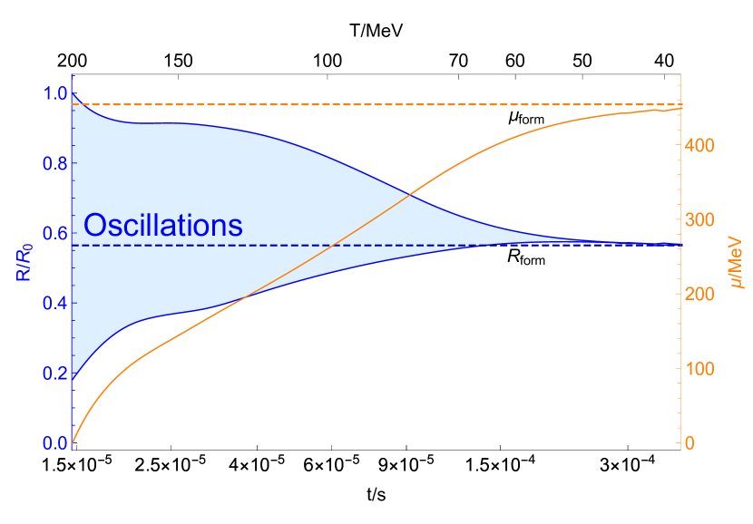
Figure 2: Numerical result of the nugget evolution. The two solid blue lines represents respectively the upper envelope and the lower envelope of $R$ oscillations. The shaded light blue region represents the numerous oscillations. The solid orange line represents the lower envelope of $\mu$ oscillations (we did not show the upper envelope and shaded region for $\mu$ oscillations to make the picture more clear). The dashed blue line and dashed orange line represents respectively $R_{\rm form}$ and $\mu_{\rm form}$ using simple analytical arguments as expressed by eqs. (56) and (57). We see that they match the numerical result of nugget evolution pretty well.

IV Baryon charge distribution

The main goal of this section is to calculate the baryon charge distribution of nuggets in the AQN scenario and compare it to the observational constraints listed in section II.2. We start in subsection IV.1 with formulating of the basic idea of the computations. In two subsections IV.2 and IV.3 which follow we study initial size and temperature distributions correspondingly. Finally, in subsection IV.4 we formulate our main results on the nugget’s distribution $dN/dB$.

IV.1 The basic idea of computations

In the present section we need a relation between initial size of the nugget $R_{0}$ formed at the temperature $T_{0}$ and its total baryon charge when the stage of formation is completed. The desired relation reads,

$$B\simeq K\cdot R_{0}^{3}T_{0}^{3},~{}~{}~{}~{}K\equiv\frac{\pi^{2}}{27\sqrt{6}}g^{\rm in}$$ (14)

see Appendix A with the detail analysis regarding relation (14). This relation implies that the total baryon charge $B$ of a stable nugget is completely determined by the initial size $R_{0}$ and the initial temperature $T_{0}$ of the closed domain wall such that $B\propto(R_{0}T_{0})^{3}$.

Eq. (14) tells us that closed domain walls with different initial radii and temperatures will eventually carry different baryonic charges $B$. Since the closed domain walls can form with different initial radii and at different temperatures ($T_{c}\lesssim T_{0}\lesssim T_{\rm osc}$), we may map these initial conditions onto a baryon charge distribution of the nuggets $dN/dB$.

According to eq. (14), the baryon charge distribution ($dN/dB$) of stable nuggets can be obtained from the initial size ($R_{0}$) and initial temperature ($T_{0}$) distributions of the closed axion domain walls which form between $T_{\rm osc}$ and $T_{c}$ as the initial stage of the nuggets. We start with the following equation

$$dN=N_{0}\cdot P\cdot f(R_{0},T_{0})\cdot dR_{0}dT_{0},$$ (15)

where $dN$ is the number of closed domain walls with the initial radius in the range $(R_{0},R_{0}+dR_{0})$ and the initial temperature in the range $(T_{0},T_{0}+dT_{0})$; $f(R_{0},T_{0})$ is two parametrical distribution function which represents the probability density of a closed domain wall with $R_{0}$ and $T_{0}$ in the above ranges. The factor $N_{0}$ is the total number of closed bubbles that form in the early Universe when $T_{a}\lesssim T_{0}\lesssim T_{c}$, while $P$ is a normalization factor to make the probability density $f(R_{0},T_{0})$ normalized to one, i.e.

$$\iint P\cdot f(R_{0},T_{0})\cdot dR_{0}dT_{0}=1.$$ (16)

The main goal of this section is to develop a technique which allows to compute $f(R_{0},T_{0})$.

To simplify our analysis we assume that all initial closed domain walls will eventually become the stable nuggets. We clarify this assumption later in the text when we compare the prediction of our construction with observational constraints. As the next step we use the relations (14) and (15), to represent the number of stable nuggets with the baryon charge less than $B$ as follows

$$N(B)=\iint_{K\cdot R_{0}^{3}T_{0}^{3}\leq B}N_{0}\cdot P\cdot f(R_{0},T_{0})\cdot dR_{0}dT_{0},$$ (17)

where $K\cdot R_{0}^{3}T_{0}^{3}\leq B$ constraints the parametrical space of the integration.

From eq. (17), we can further calculate the baryon charge distribution $dN(B)/dB$ which is the main topic of this section. Obviously, the distribution $f(R_{0},T_{0})$ which depends on $T_{0}$ and $R_{0}$ in a very nontrivial way plays a crucial rule in our calculations of the $dN(B)/dB$ distribution. The study of the function $f(R_{0},T_{0})$ can be approximately separated into two distinct pieces: one part describes the $R_{0}$- dependence, while the $T_{0}$ distribution can be incorporated separately. Next two subsections are devoted to analysis of these two different elements of the main problem.

IV.2 Initial size distribution

As discussed in section III, in the AQN model the $N_{\rm DW}=1$ domain walls are the topological defects with the axion field $\theta$ interpolating between $k=0$ ($\theta=0$) and $k=1$ ($\theta=2\pi$) branches. Although $k=0$ and $k=1$ branches correspond to the same unique physical vacuum, they effectively act as two different vacua with the same energy. The domain walls can interpolate between these (physically identical but topologically distinct) vacua, similar to a model with $V(\theta)\sim\cos\theta$ potential, when $\theta=0$ and $\theta=2\pi$ correspond to one and the same physical vacuum. Therefore, the $N_{\rm DW}=1$ axion domain walls in this scenario can be treated as $Z_{2}$ domain walls which greatly simplifies the computations.

The closed $Z_{2}$ domain walls have been observed in the simulations of $Z_{2}$-wall system [45]. In our case, it means that closed $N_{\rm DW}=1$ axion domain walls can form, which are the sources of stable nuggets as we discussed in section III. Furthermore, this analogy will provide us with more useful information about the initial size distribution of these closed bubbles. The Ref. [45] points out that the probability of forming a closed $Z_{2}$ domain wall with the initial radius $R_{0}\gg\xi$ (where $\xi$ is the correlation length of the topological defects) exponentially suppressed, $\sim\exp{(-R_{0}^{2}/\xi^{2})}$. The procedure in Ref. [45] to derive this relation is briefly reiterated as follows.

To simulate the $Z_{2}$ system in three dimensions, we first divide a big cubic volume into many small cubic cells, each of which has the length $\xi$. Then to each cell a number a number $+1$ or $-1$ is assigned at random with equal probability $p=0.5$. This is the simulation of the phenomenon that different patches (with volume $\sim\xi^{3}$) of the space during the phase transition will settle randomly with equal probability in one of the two vacua ($\theta=0$ and $\theta=2\pi$ in the case of $N_{\rm DW}=1$ axion domain walls). The domain walls lie on the boundaries between cells of opposite sign. Two neighbouring cells are connected if they have the same sign. Many connected cells can form a cluster with the same sign. The size $s$ of a cluster is defined as the number of cells in the cluster. We then can look for the size distribution of $+1$-clusters (Of course, the size of $-1$-clusters will follow the same distribution). It turns out that this is a typical problem of the percolation theory, which deals with the statistics of the clusters at different values of $p$. See Refs. [46, 47] for a review of the percolation theory.

In our case where $p=0.5$ in three dimensions, the size distribution of the finite clusters is known from the percolation theory [46], which has the following expression

$$n_{s}\propto s^{-\tau}\exp{(-\lambda s^{2/3})},$$ (18)

where $n_{s}$ is the number density of finite clusters as a function of the cluster size $s$ (the number of the cells inside a cluster). Although the distribution (18) is derived for large clusters $s\gg 1$ [46], it turns out that this relation can be extrapolated down to $s=1$ as a very good approximation [48]. As a consequence, we adopt eq. (18) for the whole spectrum $s\geq 1$ for further calculations. The two coefficients $\tau$ and $\lambda$ are $p$-dependent. According to the Ref. [48], $\lambda$ has a typical value $\sim 10$ and $\tau$ ranges from $1.5$ to $2.2$ based on the three dimensional lattice simulations. Discussing the exact values of $\tau$ and $\lambda$ at $p=0.5$ is beyond the scope of this work. Instead, we simply adopt $\lambda=10$ and $\tau=2$ for further calculations. However, as we will see, the shape of the baryon charge distribution $dN(B)/dB$ of nuggets is not sensitive to the precise numerical values of $\tau$ and $\lambda$.

The result (18) can be translated into the language of domain walls straightforwardly: The probability of forming a closed bubble with radius $R_{0}$ decreases exponentially when $R_{0}$ increases, which can be formally expressed as

$$\frac{dN}{dR_{0}}\propto\xi^{-1}\left(\frac{R_{0}}{\xi}\right)^{2-3\tau}\cdot\exp{\left[-\lambda\left(\frac{R_{0}}{\xi}\right)^{2}\right]}.$$ (19)

To derive this distribution as a function of $R_{0}$ from eq. (18), we used the relations $s\simeq R_{0}^{3}/\xi^{3}$ and $n_{s}=\frac{1}{V}\frac{dN}{ds}$ where we get rid of the simulation volume $V$ (a constant) in eq. (19). The parameter $\xi$ is the correlation length of topological defects as mentioned above, which is also set as the length of a single cell. The smallest cluster is a cell ($s\geq 1$) implying that the lowest bound of the radius of closed bubbles is $R_{0}\gtrsim\xi$. Since the relation (18) is applicable for all finite clusters $s\geq 1$ as mentioned above, we adopt eq. (19) as the size distribution of all closed bubbles $R_{0}\gtrsim\xi$.

It is very instructive to consider an oversimplified case where there is no initial temperature distribution. It can be realized if all the closed bubbles form at the same moment (at the same temperature). In this case the distribution $f(R_{0},T_{0})$ does not depend on $T_{0}$ and, according to eq. (19), can be written as $f(R_{0})=dN/dR_{0}\propto\xi^{-1}(R_{0}/\xi)^{2-3\tau}\exp{[-\lambda(R_{0}/\xi)^{2}]}$. Using eq. (14) this $R_{0}$ dependence can be translated into $\frac{dN}{dB}$ distribution:

$$\frac{dN}{dB} = \frac{dN}{dR_{0}}\frac{dR_{0}}{dB}$$

$$\propto \frac{1}{B_{\rm min}}\left(\frac{B}{B_{\rm min}}\right)^{-\tau}\exp{\left[-\lambda\left(\frac{B}{B_{\rm min}}\right)^{\frac{2}{3}}\right]},$$

where $B_{\rm min}\equiv K\cdot\xi^{3}T_{0}^{3}$. In this oversimplified model where there is no $T_{0}$ distribution, we find $dN/dB$ is greatly suppressed by the exponential factor $\sim\exp{[-\lambda(B/B_{\rm min})^{2/3}]}$. This essentially would imply that the distribution is strongly peaked at $B\approx B_{\rm min}$, while larger bubbles are strongly suppressed.

As we discuss in next subsection the $T_{0}$-dependence drastically and qualitatively changes this simplified picture. The key element is that the closed bubbles initially form at different temperatures between $T_{\rm osc}$ and $T_{c}$ as discussed above. The correlation length $\xi\sim m_{a}^{-1}$ which is inversely proportional to the axion mass $m_{a}$ drastically changes during this evolution because of the dramatic changes of the axion mass in this interval.

These profound changes completely modify the basic features of the distribution function $f(R_{0},T_{0})$, which is the subject of the following subsection. As we shall see below, the baryon charge distribution satisfies a power-law $dN/dB\propto B^{-\alpha}$ when $T_{0}$ dependence is properly incorporated, rather than follows the exponential behaviour (IV.2). This power law is consistent with parametrization (11) which has been postulated to fit the observations. Furthermore, power-law $dN/dB\propto B^{-\alpha}$ behaviour as we discuss below is not very sensitive to the parameters of coefficients $\tau$ and $\lambda$, and therefore, represents a very robust consequence of the framework.

IV.3 Initial temperature distribution and the correlation length $\xi(T)$

As we discussed in section III, the closed axion domain walls could form anywhere between $T_{\rm osc}$ and $T_{\rm c}$, see Fig. 1 to view the phase diagram corresponding this evolution. It is hard to calculate the exact $T_{0}$ distribution. It is known, though, that normally the temperature dependence enters implicitly through the correlation length $\xi(T)$ which is highly sensitive to the temperature.

To account for the corresponding modifications we adopt a conventional assumption that the correlation length is a few times the domain wall width $\xi(T)\sim m_{a}^{-1}(T)$. The axion mass is known to be a temperature-dependent function before it reaches its asymptotic value near $T_{c}$ because it is proportional to the topological susceptibility. At sufficiently high temperature $T\gg T_{c}$ one can use the instanton liquid model [52, 53] to estimate the power law $m_{a}(T)\propto T^{-\beta}$. When the temperature is close to $T\simeq T_{c}$ one should use the lattice results to account for a proper temperature scaling of the axion mass.

The recent lattice QCD result shows that $m_{a}(T)\propto T^{-\beta}$ with $\beta=3.925$ just above $T_{c}$ [54]. We then can approximate the correlation length in the entire interval as

$$\xi(T_{0})=\xi_{\rm min}\cdot\left(\frac{T_{0}}{T_{c}}\right)^{\beta},~{}~{}~{}~{}~{}T_{c}\lesssim T_{0}\lesssim T_{\rm osc}$$ (21)

where $\xi_{\rm min}\equiv\xi(T_{0}=T_{c})$ is the minimal correlation length. The same $\xi_{\rm min}$ also serves as the minimal radius that closed bubbles could have because $R\gtrsim\xi$.

In what follows we also assume the following simple model to account for the temperature variation of the ${dN}/{dT_{0}}$ distribution,

$$\frac{dN}{dT_{0}}\propto\frac{1}{T_{c}}\left[\frac{\xi(T_{0})}{\xi(T_{c})}\right]^{\delta}\propto\frac{1}{T_{c}}\left[\frac{T_{0}}{T_{c}}\right]^{\beta\delta},$$ (22)

where $\delta$ is a free parameter adjustable to shape different $T_{0}$ distributions. This parameterization has the advantage of producing a simple final expression for the baryon number distribution while still capturing the essentials of the temperature dependance. The constant $1/T_{c}$ has no special physical meaning but is introduced to balance the units of the right-hand side and the left-hand side of the relation. Perhaps the simplest case is $\delta=0$, in which case $T_{0}$ is a uniformly distributed, i.e. the probability of forming nuggets is uniform between $T_{\rm osc}$ and $T_{c}$. One should emphasize that $\delta=0$ case is still not reduced to the oversimplified example mentioned at the end of the previous subsection. This is because the temperature dependence explicitly enters through (22), but it also enters implicitly through the temperature dependence of the correlation length $\xi(T)$ in formula (19).

For positive $\delta>0$, the nuggets tend to form close to the point $T_{\rm osc}$, while for negative $\delta<0$, nuggets tend to form when the tilt becomes much more pronounced close to the QCD transition temperature $T_{c}$. Sufficiently large numerical value of $|\delta|>1$ with any sign corresponds to a very sharp, almost explosive for $|\delta|\gg 1$, increase of the probability for the axion bubble formation at $T\simeq T_{\rm osc}$ or at $T\simeq T_{c}$ depending on sign of $\delta$. At the same time $|\delta|\sim 0$ corresponds to a very smooth behaviour in the entire temperature interval (22). We, of course, do not know any properties of the distribution (22) in strongly coupled QCD when $\theta\neq 0$. Therefore, we proceed with our computations with arbitrary $\delta$ and make comments on the obtained properties of the baryon distribution $dN/dB$ as a function of unknown parameter $\delta$ in next subsection IV.4.

Combining the $T_{0}$ distribution (22) with the $R_{0}$ distribution (19), and substituting eq. (21) into eq. (19), we arrive to the following two-parametric distribution function,

$$f(R_{0},T_{0}) = \frac{1}{\xi_{\rm min}T_{c}}\cdot\left(\frac{T_{0}}{T_{c}}\right)^{3\beta(\tau-1)+\beta\delta}\cdot\left(\frac{R_{0}}{\xi_{\rm min}}\right)^{2-3\tau}$$

$$\times \exp{\left[-\lambda\left(\frac{R_{0}}{\xi_{\rm min}}\right)^{2}\left(\frac{T_{c}}{T_{0}}\right)^{2\beta}\right]},$$

$$T_{c}\lesssim T_{0}\lesssim T_{\rm osc},~{}~{}~{}~{}R_{0}\gtrsim\xi(T_{0}).$$

Notice that here we use “$=$” rather than “$\propto$”. This is because we have an extra factor $P$ in eq. (15) which serves as the normalization factor, and the constant multipliers in $f(R_{0},T_{0})$ can be collected and included into $P$.

With this expression for $f(R_{0},T_{0})$ and basic eq. (17) we can now proceed with calculation of the baryon charge distribution $dN/dB$. The corresponding results will be discussed in the next subsection.

IV.4 The $dN/dB$ distribution. Results.

Substituting eq. (IV.3) into eq. (17), one can explicitly compute the function $N(B)$ and the distribution $dN/dB$. In what follows it is convenient to introduce the following dimensionless variables: the baryon charge $b=B/B_{\rm min}$ of the nugget measured from its minimum value $B_{\rm min}=K\xi_{\rm min}^{3}T_{c}^{3}$; the relative size $r=R_{0}/\xi_{\rm min}$ of the nugget measured from its minimum size $\xi_{\rm min}$; the relative temperature $u=T_{0}/T_{c}$ during formation evaluation in units of $T_{c}$.

In terms of these dimensionless variables the desired distribution ${dN}/{dB}$ can be represented as follows

$$\frac{dN}{dB}=\frac{N_{0}P}{3B_{\rm min}}\cdot\left(\frac{1}{b}\right)^{\tau}$$

$$\times \int_{1}^{b^{\frac{1}{3(\beta+1)}}}du~{}\left[u^{3(\beta+1)(\tau-1)+\beta\delta}{\rm e}^{-\lambda b^{{2}/{3}}u^{-2(\beta+1)}}\right],$$

see Appendix B with all technical details.

One can easily estimate the integral (IV.4) by observing that it is saturated for very large $b\gg 1$ by $u_{\rm sat}$ of order

$$u_{\rm sat}\sim\left[\lambda b^{2/3}\right]^{\frac{1}{2(\beta+1)}}\sim b^{\frac{1}{3(\beta+1)}},~{}~{}~{}~{}~{}b\gg 1$$ (25)

when the exponential factor in (IV.4) assumes a value of order one. Substituting the expression back to eq. (IV.4) one arrives to the following asymptotical behaviour for the distribution

$$\frac{dN}{dB}\propto B^{-\alpha},~{}~{}B\gg B_{\rm min},$$ (26)

where the final result is expressed in terms of the physical baryon charge $B$ rather than in terms of the dimensionless parameter $b$. Parameter $\alpha$ here is defined precisely in the same way as it is defined in the observational fitting formula (11).

The exponent $\alpha$ entering (26) can be approximated in the limit $B\gg B_{\rm min}$ as follows

$$\alpha\approx 1-\frac{\beta\delta+1}{3(\beta+1)}\sim 1-\frac{\delta}{3},$$ (27)

where in the last step we ignored the factors of order one in comparison with known (and very large) value of $\beta\simeq 4$ to simplify qualitative discussions below. The approximate analytical formula (26) at very large $B\gg B_{\rm min}$ is in perfect agreement with numerical analysis presented in Appendix B.

The behaviour (26) is amazingly simple and profoundly important result. Indeed, it shows that the exponential suppression is replaced by the algebraic decay (26) which is consistent with observational fitting formula (11). The “technical” explanation for this to happen is that the integral (IV.4) is saturated by $u_{\rm sat}$ when the exponential factor in (IV.4) assumes a value of order one. In terms of the physical parameters it is related to the fact that exponential suppression (IV.3) due to the large size $R_{0}$ is effectively removed by a strong temperature dependence with very large beta function $\beta$. Integration over entire temperature interval eventually leads to the algebraic decay (26).

Another important property of the expression (26) is that the final result for the slope (27) is not very sensitive to the parameters $\lambda$ and $\tau$. The total normalization factor of course is very sensitive to these parameters as discussed in Appendix B. It is also not very sensitive to the well known parameter $\beta\approx 4$ as long as it is relatively large. The slope $\alpha$ is mostly determined by $\delta$ which may have any sign and effectively describes the temperature interval where the bubbles are produced with the highest efficiency. The fitting models (11) based on observations which were discussed in Section II can be reproduced with negative $\delta<0$. The negative sign of $\delta$ as we previously mentioned corresponds to the preference of the bubble formation close to $T_{c}$ where the axion potential tilt becomes much more pronounced. Furthermore, a model with $\alpha\simeq 2$ corresponds to $\delta\simeq-3$ (strongly peaked at $T\simeq T_{c}$), while another model with $\alpha\simeq 1.2$ corresponds to a more smooth distribution of ${dN}/{dB}$ over the entire temperature interval with $\delta\simeq-1$ corresponding to mild preference of the bubble formation at $T\simeq T_{c}$.

The last comment we want to make is about the largest possible size of nuggets. According to percolation theory, there is no upper limit on the size of finite clusters (closed domain walls). However, the shape of large clusters may not be perfectly spherical (in 3D) while our computations are based on assumption of exact spherical symmetry of the formed bubbles. Furthermore, the radius for non-symmetric bubbles is defined in average sense for large closed clusters, see e.g.  [47] for more details. The deviation from the ideal spherical shape makes the large collapsing closed domain walls to fragment with high probability into smaller pieces and thus could significantly suppress the possibility of forming large nuggets. The detailed calculations of the suppression effect from the irregular shape for large clusters is hard to carry out and also well beyond the scope of the present work. However, we may introduce a cutoff $B_{\rm cut}$ to roughly account for this extra suppression. Above $B_{\rm cut}$, no nuggets can form from the collapse of closed axion domain walls. This parameter turns out to be useful when we later calculate the total number of nuggets.

We conclude this section with the following remark. The main result of our analysis is expressed as (26) with the slope (27). This formula represents the baryon charge distribution immediately after the formation period is complete when the baryon to photon ratio $\eta$ assumes its present value (5). This “primordial” distribution of the nuggets is the subject of a long evolution in hot plasma which may modify the properties of $dN/dB$. This problem of “survival” of the primordial nuggets is the subject of the next section.

V Survival of the Primordial Distribution

After the AQN have formed at $T\approx 40$ MeV the process of “charge separation” is essentially complete and the plasma surrounding the nuggets contains exclusively protons, neutrons, electrons and positrons. A nugget composed of matter will gradually collect electrons into its electrosphere as the plasma cools but apart from this will essentially remain in its initial form. The surface layer of electrons contribute negligibly to the total mass so that the distribution of nugget masses remains essentially identical to the primordial distribution discussed above. However, the AQN composed of antimatter, which are present in larger numbers, will be subject to a much more complicated evolution. The details of this process will be laid out below, but we first give a general overview of the evolution of the antimatter AQN mass distribution.

Initially the plasma surrounding the AQNs is dominated by electrons and positrons which are roughly as abundant as the photons, i.e. $n_{e}\simeq n_{e^{+}}\simeq n_{\gamma}\sim T^{3}$. During this phase the electrosphere captures positrons into those states for which the binding energy is above the plasma temperature and expands similar to the case of a matter nugget. However, once the temperature drops below the electron mass $T\leq m_{e}$ the electrosphere can no longer capture free positrons at a rate sufficient to compensate for annihilations. Below this temperature the electrosphere will begin to capture free protons which, if they stay bound to the nugget for a sufficient period of time, will eventually annihilate with the central quark matter.

The process of capturing protons become much more pronounced after the temperature drops to $T\approx 20$ keV when the dominant portion of the positrons in the plasma get annihilated, while the number density of electrons and protons become equal, i.e. $n_{e}\approx n_{p}\sim\eta T^{3}$. However, even at this temperature, as we discuss below, only a very tiny portion of the AQN’s baryon charge will be annihilated, such that mass distribution still remains essentially unaffected by the unfriendly environment in form of the hot plasma.

Finally, after recombination at $T\leq 1$ eV the surrounding matter is largely neutral and at much lower densities. During this time matter (primarily in the form of neutral hydrogen) will continue to collide with the antimatter AQN with some probability of annihilation but at a relatively low rate. The rare events of annihilation during the present time lead to a number of observable effects as reviewed in Section II.2.

At each phase of evolution the scattering rate of baryons on the nugget (and thus the probability of an annihilation) scales with the cross-section of the nugget. This is at least approximately true even in the case where long range electrical effects must be considered as the nuggets’ electrical charge is itself a surface effect. As such any change in the mass distribution should be expected to show a $\Delta M/M\sim\sigma/M\sim B^{-1/3}$ behaviour.

The following sections will trace the evolution of the mass distribution from formation to the present day. Specifically, in next section VI we study the evolution of the nuggets in very hot plasma before BBN epoch. In section VII we analyze the AQN evolution before the recombination, while in section VIII we the evolution of the nuggets after the recombination including the period of the galaxy formation. Finally, in section IX we study the evolution of the AQNs at present day Universe. We will demonstrate that, for a range of physically interesting parameters, the initial population of AQN will survive until the present day as a population consistent with all observational constraints and with the parameter space allowed for the axion mass and the AQN’s baryon charge $B$ as discussed in Section II.2.

VI Pre-BBN Evolution

The AQN complete formation and settle into a stable colour superconducting phase at a temperature of approximately $T_{\rm form}\approx 40$ MeV, see Fig.1. Once this transition is complete the AQN will cease accreting mass and annihilation with the free baryons in the plasma will become the dominant process. However, annihilation between an energetic free baryon and the quark content of the AQN is highly nontrivial process as we discuss below.

We start with the estimates of the collision rate in pre-BBN epoch. The corresponding rate between an AQN and the baryons of the surrounding plasma is,

$$\Gamma_{\rm col}=4\pi R^{2}n_{B}v_{B}=4\pi R^{2}\frac{2\zeta(3)}{\pi^{2}}\eta\left(\frac{T}{\hbar c}\right)^{3}\sqrt{\frac{2T}{m_{p}}}c$$ (28)

where the baryon number density in plasma $n_{B}$ can be approximated as $n_{B}\sim\eta T^{3}$. The total number of collisions during this time period is saturated by the highest temperature $T_{\rm form}\simeq 40~{}{\rm MeV}$ and can be estimated as follows

$$N_{\rm col}=\int dt~{}\Gamma=\int_{0}^{T_{\rm form}}dT~{}\frac{dt}{dT}~{}\Gamma_{\rm col}$$ (29)

$$\approx 3\times 10^{25}\left(\frac{T_{\rm form}}{40~{}{\rm{MeV}}}\right)^{1.5}\left(\frac{R}{10^{-5}{\rm{cm}}}\right)^{2}$$

where we have used the relation $t\sim T^{-2}$ to change to a temperature integration.

While the number of collisions (29) is comparable with the total baryon charge $B$ of a nugget, the probability of annihilation is quiet small. Instead, the most likely interaction of any incident matter with the nugget is total reflection due to a number of reasons: the sharp boundary between hadronic and CS phases such that only a very small fraction $\kappa(T)\ll 1$ of collisions represented by (29) will result in an annihilation. We refer to Appendix C for order of magnitude estimates supporting the main claim that $\kappa(T)\ll 1$. A more precise vale is not essential for our arguments which follow.

So long as the electrons and positrons remain relativistic (and thus present in numbers comparable to the photons) all long range interactions are effectively screened and the cross section appearing in expression (28) is purely the physical size of the AQN. As such the estimate (29) holds until much lower temperatures when the positrons have fully annihilated (which approximately occurs at $T\approx 20$ keV) and longer range interactions become possible. The estimate (29) implies that the number of annihilation events does not modify the primordial spectrum of the AQNs discussed in Section IV.4 because the relative number of annihilation events is very small, i.e. $(\kappa N_{\rm col})/B\sim\kappa\ll 1$.

While the baryon charge annihilation events are strongly suppressed by the factor $\kappa\ll 1$ the $e^{+}e^{-}$ annihilation events involving particles from AQN’s electrosphere are much more numerous and unsuppressed. One may therefore wonder if the energy injection by these annihilation events may impact the conventional thermal history of the Universe. The answer is “no” as simple estimates for the extra injected energy (due to the annihilation events with AQNs) show. Indeed, the relative injection energy due to AQNs at temperature $T$ in comparison with average thermal energy $(Tn_{\rm e})$ of the plasma can be estimated as follows,

$$\frac{1}{(Tn_{\rm e})}\frac{dE}{dV}\sim\frac{\left(R^{2}T^{2}\right)\eta}{\alpha^{2}\langle B\rangle}\sim 10^{-19}\left(\frac{T}{1~{}\rm MeV}\right)^{2}.$$ (30)

see appendix in ref. [12]. The basic reason for this tiny rate is the same as discussed before: the cross section is proportional to $R^{2}\sim B^{2/3}$, while the number density of the nuggets is proportional to $\eta/\langle B\rangle$ which results in a strong suppression rate (30). It is clear that such small amount of energy injected into the system will be quickly equilibrated within the system such the standard pre-BBN cosmology remains intact. In other words, the conventional equation of state, and conventional evolution of the system is unaffected by presence of AQNs.

VII Post-BBN evolution

At temperatures below $T_{\gamma}\simeq m_{e}$ the electrons and positrons begin to annihilate causing their density to fall as $\sim e^{-m_{e}/T}$ until a major portion of the positrons get completely annihilated while the number densities for electrons $n_{e}$ and protons $n_{B}$ become approximately equal at $T_{*}\simeq 20$ keV. This is the consequence of the same “charge separation” effect (replacing the “baryogenesis” in AQN framework) when more antimatter than matter is hidden in form of dense nuggets as reviewed in Section II.

This regime when the AQNs are present in the plasma at $T_{*}\simeq 20$ keV has been recently discussed in [4] in quite different context and for very different purposes. To be more specific, it has been shown that the primordial abundance of Li and Be nuclei will be depleted in comparison with conventional BBN computations. This effect represents the resolution of the “primordial Li puzzle” within AQN framework.

The main goal of the present work is very different, though the plasma regime surrounding the AQNs is the same with $T\lesssim T_{*}$. In the present paper we study the survival pattern of the nuggets themselves, in contrast with the studies in [4] when the main question was the analysis of relative densities $\delta n_{Z}/n_{Z}$ of primordial nuclei with charge $Z$ as a result of the AQN presence in plasma.

We start our analysis by highlighting the basic features of the AQN electrosphere in the regime $T\lesssim T_{*}$ using simple qualitative arguments. Later in the text we will support these arguments by providing some analytical formulae. At $T\approx T_{*}$ when the external positron density essentially vanishes the boundary conditions for the AQNs’ electrosphere fundamentally change resulting in a new charge distribution. Below $T_{*}$ some fraction of the electrosphere positrons will be replaced by protons to fit with the new long distance, proton dominated boundary condition. The exact proton to positron ratio of the electrosphere will be determined by the rate at which captured protons are annihilated by the nuggets, positrons are annihilated by external electrons and the rate at which beta-processes can replace near surface positrons.

Further from the quark surface the positrons are more weakly bound and thermal behaviour becomes important to the distribution. In this regime the density as a function of height scales as [24, 25],

$$n_{e^{+}}=\frac{T_{N}}{2\pi\alpha}\frac{1}{\left(z+\bar{z}\right)^{2}},~{}~{}~{}\bar{z}^{-1}\approx m_{e}\sqrt{2\pi\alpha}\left(\frac{T_{N}}{m_{e}}\right)^{1/4}$$ (31)

where the approximate value of $\bar{z}$ is taken from matching this solution to the numerical solution from higher densities.

The main observation here is that a $T\neq 0$ environment leads to ionization of the loosely bound positrons such that the antinuggets will be in a negative charged configuration with charge $-Q$ estimated as follows

$$Q\simeq 4\pi R^{2}\int^{\infty}_{z_{0}}n(z)dz\sim\frac{4\pi R^{2}}{2\pi\alpha}\cdot\left(T\sqrt{2m_{e}T}\right)~{}~{}~{}~{}~{}$$ (32)

where we assume that some loosely bound positrons will be stripped off the electrosphere as a result of non-zero temperature. This negative charge of the antinugget implies that the protons from the plasma might be captured by the nugget by screening the charge (32). It obviously implies that the effective cross section for capturing of the protons $\sim 4\pi R_{\rm cap}^{2}(T)$ will be drastically larger than $4\pi R^{2}$ from our previous estimates (28), (29) when the electrosphere is entirely made of the positrons, not protons.

In principle the distribution of protons surrounding the nugget should be determined through a Thomas-Fermi computation similar to that performed in [25] but allowing for the presence of protons as well as positrons and using the early universe plasma density as the $r\rightarrow\infty$ boundary condition. However, for present order of magnitude estimates we will assume a simple power law scaling with exponent $p$,

$$n_{p}(r)=n_{0}\left(\frac{R}{r}\right)^{p}$$ (33)

with the normalization $n_{0}$ set to match the total charge given in expression (32). This assumption is consistent with our numerical studies [25] of the electrosphere with $p\simeq 6$ for positrons. It is also consistent with conventional Thomas-Fermi model at $T=0$, see [4] for references and details. We keep parameter $p$ to be arbitrary to demonstrate that our main claim is not very sensitive to our assumption on numerical value of $p$. With these assumptions the baryon number density $n_{0}$ in close vicinity of the nugget can be estimated as follows,

$$n_{0}=\frac{p-3}{4\pi R^{3}}Q.$$ (34)

One should note that the behaviour of the proton cloud may deviate significantly from expression (33) at very small and very large radii, however we simply want to determine the approximate scale over which electromagnetic effects will act. In this context the simple form of expression (33) should be sufficient. This behaviour will continue until the proton density matches that of the surrounding plasma which gives us a radius for the over density of protons surrounding by the nugget.

$$\left(\frac{R_{\rm cap}}{R}\right)^{p}\sim\left(\frac{n_{0}}{\eta n_{\gamma}}\right)\sim 10^{12}\cdot\left(\frac{20~{}{\rm keV}}{T}\right)^{3/2}.$$ (35)

This increase in the effective scattering length of the nuggets will boost the number of interactions and may result in an increased annihilation rate. Most importantly these captured protons will spend an extended amount of time near the surface of the AQN giving them an increased opportunity to annihilate. Again, we stress that this increased rate of proton capture is effective only after the positrons are fully annihilated and the protons are the only positive charge carriers in the plasma which happens at $T\simeq T_{*}\simeq 20$ keV.

In particular for $p\simeq 6$ the effective capture distance $R_{\rm cap}$ is of order

$$R_{\rm cap}\simeq 10^{2}\cdot\left(\frac{20~{}\rm keV}{T}\right)^{\frac{3}{2p}}R,$$ (36)

which of course drastically changes the collision rate as will be estimated below. The scaling (36) holds as long as the thermal equilibrium between the nuggets and surrounding plasma is maintained. Formula (36) breaks down at sufficiently large $R_{\rm cap}$ when the power law scaling (33) is replaced by the exponential behaviour due to the Debye screening. Numerically, the Debye screening becomes operational at $R\simeq 10~{}R_{\rm cap}$ at $T\simeq 20$ keV, see Appendix A in [4].

We may now perform the same estimates as in expressions (28) but using the larger capture cross section of equation (36), i.e.

$$\Gamma_{\rm col}(T)=4\pi R_{\rm cap}^{2}(T)n_{B}(T)v_{B}(T).$$ (37)

The total number of collisions during this time is saturated by the highest temperature $T\simeq T^{*}$ such that the integral can be estimated as follows

$$N_{\rm col}(T)=\int_{0}^{T_{*}}dT~{}\frac{dt}{dT}\Gamma_{\rm col}(T)$$

$$\sim 10^{24}\left(\frac{T}{20~{}\rm{keV}}\right)^{(\frac{3}{2}-\frac{3}{p})}\left(\frac{R}{10^{-5}{\rm{cm}}}\right)^{(2-\frac{2}{p})}$$

where we use $p=6$ for numerical estimates. The expression (VII) represents a full analog of the estimate (29) obtained for pre-BBN epoch.

While the number of scatterings occurring in this low temperature regime is slightly below the number occurring just after nugget formation as estimated in equation (28) we expect the evolution of the AQN baryon number to be dominated by these low energy collisions in which the AQN and baryonic matter temporarily form a bound state. This is because, as argued above, collisions at tens of MeV are highly likely to result in elastic scattering while electromagnetically bound protons have a much larger opportunity to come into overlap with the quark modes of the colour superconductor and eventually annihilate.

The similarity in the total number of collisions in the estimates (29) and (VII) at $T_{\rm form}\simeq 40~{}{\rm MeV}$ and $T_{*}\simeq 20$ keV correspondingly can be easily understood from the following simple observations. The baryon number density in plasma scales as $T^{3}$, the proton’s velocity in plasma scales as $T^{1/2}$, the cosmic time scale as $T^{-2}$. All these factors result in drastic changes in the rate between $T_{\rm form}\simeq 40$ MeV and $T_{*}\simeq 20$ keV with approximate suppression factor: $(T_{*}/T_{\rm form})^{3/2}\sim 10^{-5}$. However, these substantial suppression in the temperature is mostly compensated by enhancement in effective cross section $(R_{\rm cap}/R)^{2}\sim 10^{4}$, see estimate (36). These two effects work in opposite directions which explains our estimates for the collision rates (VII) and (29) being numerically close.

We summarize this section with the following comment. The total number of collisions (VII) is still much smaller than a typical baryon charge $\langle B\rangle\sim 10^{25}$ of the nuggets, such that the majority of the nuggets will survive the post-BBN epoch as only small portion of the collisions will eventually lead to the annihilation events. Therefore, from these estimates we conclude that the post-BBN epoch does not modify the primordial spectrum of the AQNs.

At this point a thoughtful and careful reader may wonder how it could happen that the number of annihilation events estimated above is sufficiently small that all nuggets with $B>10^{24}$ can easily survive the unfriendly hot and dense environment of early universe according to estimates (VII) and (29). At the same time, it has been argued recently in [5, 28, 6] that the nuggets of all sizes will experience complete annihilation in the solar corona when the AQNs enter the solar atmosphere. How these two claims could be consistent? We refer the readers to Appendix D specifically addressing this question where we emphasize a number of crucial differences between the two cases.

The only comment we would like to make here is that the drastic enhancement of the rate of annihilation in solar corona is due to the propagation of the AQN with supersonic speed (above the escape velocity $v>600$ km/s at the solar surface) in the ionized plasma with a very large Mach number $M=v/c_{s}\simeq 10$, where $c_{s}$ is the speed of sound in the solar atmosphere. It is well known that a moving body with such a large Mach number will inevitably generate a shock wave and accompanying it a temperature discontinuity with turbulence in vicinity of a moving body. As a result of this complicated non- equilibrium dynamics the effective cross section may be drastically increased in the course of shock wave propagation due to the capture (with subsequent annihilation) of a large number of ions from plasma. These features of the AQNs in the solar corona should be contrasted with AQN’s adiabatic evolution in the plasma of the early Universe with its relatively slow evolution.

VIII Post-recombination evolution

The integral (VII) is saturated by the highest possible value $T\simeq T_{*}\simeq 20$ keV because the largest collision rate occurs precisely at that time. As the temperature slowly decreases due to the Universe’s expansion one should not expect any dramatic changes until the recombination epoch at $T\simeq 0.3$ eV. At this point the universe becomes neutral and the scattering cross section of matter with the AQN no longer receives a boost from electromagnetic effects analogous to (36). Therefore, these generic arguments suggest that the collision rate diminishes even faster after recombination impling that the size distribution of the AQN essentially does not change during that epoch. These generic arguments obviously do not apply to violent environments during galaxy or star formation (which occur during this epoch) and which will be analyzed later in this section.

In spite of this relatively dilute environment, the rare events of annihilation of the AQNs with surrounding baryons still occur even at such low density. The corresponding radiation due to the annihilation processes, while negligible in comparison with the dominating CMB radiation, may nevertheless leave some imprints which could be observed today, as argued in [12]. This is due to some specific features of the spectrum characterizing the AQN annihilation events: the low energy tail of the radiation due to the annihilation processes with the nuggets has spectrum $\sim\ln\nu$ which should be contrasted with conventional CMB black body radiation characterized by $\nu^{2}$ behaviour at low $\nu\ll T$, see [12] for the details.

As we mentioned above, the violent environment during the galaxy or star formation requires a special treatment because it may potentially change the generic argument that this epoch is essentially irrelevant to the AQN’s survival pattern. In what follows we compare the environment during the galaxy and star formation with corresponding features in the solar corona (where it has been argued that complete annihilation of the AQNs occurs) in the context of the AQN annihilation rate. The outcome of this comparison and corresponding conclusion will be formulated at the very end of this section.

The complete annihilation of the AQNs in the solar corona as discussed in [5, 6] and reviewed in Appendix D is the direct consequence of a few factors:
1. relatively large density in the transition region $n\sim 10^{11}{\rm cm^{-3}}$;
2. very large velocity of the nuggets on the solar surface, $v>v_{\odot}=\sqrt{2GM_{\odot}/R_{\odot}}\simeq 600$ km/s. This is of course a result of strong gravitational forces $\sim M_{\odot}$ localized on a relatively small distance $R_{\odot}$;
3. large velocity $v$ greatly exceeds the speed of sound $c_{s}\simeq\sqrt{T/m_{p}}$. It implies that the Mach number is very large, $M\equiv v/c_{s}\gg 1$ such that shock waves inevitably form;
4. high ionization of the plasma due to large temperature $T\simeq 10^{6}$K in the transition region.

The combination of these factors lead to complete annihilation of the AQNs as reviewed in Appendix D. While individual (violent) condition from the list above may emerge during the galaxy or star formation, the combination of all 4 elements does not occur, in general, during this epoch. Therefore, we do not expect any considerable modification of the size distribution of the nuggets after the recombination.

Indeed, the baryon density during the structure formation epoch does not exceed $n_{B}\sim 1~{}{\rm cm^{-3}}$. Furthermore, the typical velocities of particles in the gas are the same order of magnitude as the speed of sound, i.e. $v\sim c_{s}\sim 10^{2}~{}{\rm km/s}$ such that one should use a conventional formula for estimation of the collision rate without any additional enhancement factors related to Mach number $M$, i.e.

$$\Gamma_{\rm col}\sim 4\pi R^{2}n_{B}v_{B}\sim 10^{-2}s^{-1}(\frac{n}{{\rm 1~{}cm^{-3}}})(\frac{v}{100{\rm km/s}}).$$

The total number of collisions $N_{\rm col}$ during the Hubble time $H^{-1}$ at redshift $z\sim 10$ is of order

$$N_{\rm col}\sim\Gamma_{\rm col}\cdot H^{-1}\sim 10^{14}\left(\frac{n}{{\rm 1~{}cm^{-3}}}\right)\left(\frac{v}{100~{}{\rm km/s}}\right),~{}~{}~{}$$ (39)

which represents a tiny portion of the average baryon charge $\langle B\rangle\sim 10^{25}$ of a nugget. Furthermore, even if in some small regions the relative velocities of the AQNs and baryons exceed the speed of sound $c_{s}$ it does not lead to shock wave formation similar to our discussions in the solar corona (reviewed in Appendix D). This is because the shock wave phenomenon is based on effective description of the system when the hydrodynamical description is justified, which implies that a typical distance between the particles $\sim n^{-1/3}$ must be much smaller than the size of a moving body $\sim R$. This approximation is obviously badly violated for the AQNs during the structure formation epoch. Therefore, according to our estimate $N_{\rm col}\ll\langle B\rangle\sim 10^{25}$, and we conclude that the size distribution of the AQNs is not modified during the era of structure formation.

A similar conclusion also holds for another violent epoch (star formation) which could also potentially modify the AQN size distribution. The corresponding analysis can be separated in two different stages: the final stage of formation when typical parameters are similar to our analysis of the Sun, and the initial stage of star formation characterized by the density ranging from $n\sim 10^{15}{\rm cm^{-3}}$ to $n\sim 10^{0}{\rm cm^{-3}}$ depending on size of infall cloud ranging from $r\sim 10^{-1}{\rm AU}$ to $r\sim 10^{6}{\rm AU}$, see [56].

We start our estimates from the final stage of formation when the stars assume their final form. In this case all the nuggets which will be captured by a star will be completely annihilated similar to our studies of the sun. However, the portion of the AQNs which will be captured by the stars is very tiny in comparison with total number of nuggets. The corresponding portion of the affected nuggets can be estimated in the terms of the capture impact parameter $b_{\rm cap}$ which is typically only few times the star’s size $R_{\star}$.

$$b_{\rm cap}\simeq R_{\star}\sqrt{1+\gamma_{\star}},~{}~{}~{}~{}\gamma_{\star}\equiv\frac{2GM_{\star}}{R_{\star}v^{2}},$$ (40)

where $v\sim 10^{-3}c$ is a typical velocity of the nuggets far away from the star. The rate of the total mass annihilation $dM_{\rm ann}/dt$ of all nuggets captured (and consequently annihilated) by the star can be estimated as follows

$$\frac{dM_{\rm ann}}{dt}\sim 4\pi b^{2}_{\rm cap}v\rho_{\rm DM}\simeq 3\cdot 10^{30}\left(\frac{v}{10^{-3}c}\right)\frac{m_{p}}{\rm s},$$ (41)

where we used the solar parameters for the numerical estimates and assumed that $\rho_{\rm DM}$ is saturated by the AQNs. The upper limit of total mass annihilated by a single star can be estimated by multiplying (41) to the total life time of star which can be approximated as $H^{-1}$, i.e.

$$M_{\rm ann}\leq\frac{dM_{\rm ann}}{dt}\cdot H^{-1}\sim 10^{48}m_{p}\sim 10^{21}{\rm kg}.$$ (42)

Estimate (42) should be compared with total mass of the star $M_{\star}\sim M_{\odot}\sim 10^{30}{\rm kg}$. As the stars represent only a fraction of the total baryonic matter of the Universe, and the DM is 5 times the total baryonic matter, one can infer from (42) that the annihilated portion of DM (due to the capturing by stars) represents only a small portion $\lesssim 10^{-10}$ of the total dark matter material of the Universe.

We now turn to the estimates of the AQN annihilation pattern during the initial stage of star formation. In this case the DM nuggets passing through infall cloud experience the annihilation events. The corresponding total annihilated baryon charge for a single nugget (as a result of this passage) can be estimated as follows,

$$N_{\rm col}\sim\pi R^{2}n_{B}L\sim 10^{9}\cdot(\frac{n_{B}}{{\rm 1~{}cm^{-3}}})\cdot(\frac{L}{10^{6}AU}),$$ (43)

which represents a tiny portion of the average baryon charge $\langle B\rangle\sim 10^{25}$. In estimate (43) we used the most generic configurations when AQNs enter a large region with $L\sim 10^{6}$AU characterized by $n_{B}\sim{\rm 1~{}cm^{-3}}$, while passage of the nuggets through small well-localized region $L\sim 10^{-1}$ AU with high density $n_{B}\sim{\rm 10^{15}~{}cm^{-3}}$ is highly unlikely as it represents a very small portion of the total AQN flux. But even in this case the total number of annihilation events $N_{\rm col}\sim 10^{17}$ remains small in comparison with average baryon charge $\langle B\rangle\sim 10^{25}$.

We conclude this section with the following comment: The violent events such as galaxy formation or star formation after recombination do not drastically modify the size distribution of the nuggets, similar to our previous analysis devoted to the different epochs in the Universe evolution. The basic reason for this conclusion is that the nuggets which can experience compete annihilation represent only small portion of the entire population according to (42), while the majority of the nuggets will loose a very tiny portion of their baryon charge during the Hubble time according to (39).

IX Present Day Mass distribution

After recombination the size distribution of the AQN to be essentially fixed until the present day. We may formulate the change in baryon number as a result of post-formation annihilation as,

$$\Delta B=f_{1}N_{\rm col}(T>T_{*})+f_{2}N_{\rm col}(T<T_{*})$$ (44)

where $f_{1}$ and $f_{2}$ are the fractions of collisions in the positron dominated and proton dominated phases which result in the annihilation of a unit of baryon charge from the AQN with the collision rates taken from expressions (29) and (VII) correspondingly. If we assume an original nugget distribution defined by $B_{\rm min}$, $B_{\rm cut}$ and $\alpha$ as discussed in section IV.4 we may use expression (44) to translate the distribution formed above $T\approx 40$ MeV to a present day mass distribution. Note that, since $R\propto B^{1/3}$ the first term in expression (44) scales as $B^{2/3}$ according to (29), while the second scales as $B^{5/9}$ according to (VII).

We may then write the late time baryon number distribution based on result (26) obtained from percolation theory as follows,

$$\frac{dN}{dB}=N_{0}\left(\frac{B_{\rm min}}{B}\right)^{\alpha},~{}~{}B\gg B_{\rm min},$$ (45)

where $B$ is the present day baryon number of the AQN and we have ignored the small portion $\Delta B$ related to the annihilation processes as discussed above.

For a given environment the constant $N_{0}$ may be fixed if the AQNs are assumed to provide the entire dark matter mass. We also assume that one and the same $\alpha$ describes the mass distribution for all values of $B$. It may or may not be a correct assumption as some nanoflare’s models fit the solar corona heating with different exponents $\alpha$ for small and large values of $B$, see below with additional comments.

With the assumptions just formulated one can represent $\rho_{\rm DM}$ as follows,

$$\rho_{\rm DM}=\int^{B_{\rm cut}}_{B_{\rm min}}m_{p}B\frac{dN}{dB}dB$$ (46)

where ${dN}$ has a physical meaning of the AQN number density per unit volume per baryon charge interval $dB$, while $m_{p}B({dN}/{dB})$ has physical meaning of the mass density per unit volume hidden in form of the nuggets with baryon charge from $B$ to $B+dB$. The relation (46) allows us to solve for the normalization factor in expression (45) for different exponents $\alpha$’s:

$$N_{0} = (\alpha-2)\frac{\rho_{\rm DM}}{m_{p}B_{\rm min}^{2}}~{}~{}~{}~{}~{}~{}~{}~{}~{}~{}~{}~{}~{}~{}~{}\alpha>2$$ (47)

$$N_{0} = \frac{\rho_{\rm DM}}{m_{p}B_{\rm min}^{2}{\rm{ln}}(B_{\rm cut}/B_{\rm min})}~{}~{}~{}~{}~{}~{}\alpha=2$$

$$N_{0} = (2-\alpha)\frac{\rho_{\rm DM}}{m_{p}B^{2}_{\rm cut}}\left(\frac{B_{\rm cut}}{B_{\rm min}}\right)^{\alpha}~{}~{}\alpha<2$$

where we have again assumed that $\Delta B\ll B$ represents a small fraction of the initial baryon number as argued to be the case in previous sections VI and VII.

Note that $\alpha=2$ marks the slope at which the distribution transitions from being mass dominated by the bottom end to the higher end. Distributions with $\alpha>2$ are largely defined by the mass scale $B_{\rm min}$ while the typical mass scale for shallower sloped distributions with $\alpha<2$ is dominated by $B_{\rm cut}$.

We may now ask, given the profile of expression (45) what range of parameters are consistent with observational constraints discussed in Section II.2? As argued above we expect that $f_{1}<<f_{2}$ so that the majority of annihilations occur below $T\sim 20$ keV, if this is the case then the parameter space of the AQN model may largely be defined by four variables; $B_{\rm min}$, $B_{\rm cut}$, $\alpha$ and $\Delta B\sim f_{2}$. As discussed in section IV.4 these parameters are not well constrained from the theoretical end. Indeed, while the theoretical analysis predicts a generic power law behaviour (26) the numerical value for the exponent $\alpha$ is expressed in terms of parameter $\delta$ according to eq. (27) which itself describes some features of the bubble’s formation during the QCD transition at $T\sim T_{c}$, which are basically unknown in strongly coupled QCD.

From the observational end the constraints are less trivial and much more interesting. First of all, there are constraints on $\alpha$ which come primarily from solar data. As we discussed in section II.2.4, the solar corona measurements are sensitive to the full distribution rather than simply the average value $\langle B\rangle$. If the nuggets are to offer an explanation to the solar heating problem as argued in [5, 28, 6] then we require that the majority of heat input comes from lower energy unobservable events and thus must have $\alpha>2$. This option is consistent with analysis of the nanoflare distribution performed in ref.[30] where the authors claim that the best fit to the data is achieved with $\alpha\simeq 2.5$ while numerous attempts to reproduce the data with $\alpha<2$ were unsuccessful.

Another option advocated in ref. [31] is that the nanoflare distribution consists two different exponents: The events below $E\leq 10^{24}{\rm erg}$ are described by $\alpha\simeq 1.2$ while the higher energy events with $E\geq 10^{24}{\rm erg}$ are described by $\alpha\simeq 2.5$. In terms of baryon charge distribution (45) the model [31] corresponds to the nugget mass distribution with $\alpha\simeq 1.2$ and cutoff scale near $B_{\rm cut}\sim 10^{27}$. The higher mass nuggets with $B_{\rm cut}\geq 10^{27}$ are described by $\alpha\simeq 2.5$.

Assuming that the distribution (45) can be approximately used in close vicinity of $B_{\rm min}$ one can relate the average baryon number $\langle B\rangle$ and $B_{\rm min}$ as follows

$$\langle B\rangle\approx\frac{\alpha-1}{\alpha-2}B_{\rm min},~{}~{}~{}\alpha>2$$ (48)

so that, for any $\alpha>2$ the average $\langle B\rangle$ and $B_{\rm min}$ are at the same scale. One should not literally use the relation (48) as the distribution (45) cannot be numerically trusted in close vicinity of $B_{\rm min}$, see footnote 17 with comments. If one uses the observational constraint on $\langle B\rangle$ from (8) one can impose the constraint on $B_{\rm min}\gtrsim 10^{24}$ from (48).

For the AQN population to survive as high mass dark matter candidates we require $B_{\rm min}>\Delta B$ which, from expression (VII), suggests a lower bound below $\sim 10^{24}$ though, as argued above this scale considers the number of collisions between background plasma with an AQN rather than the number of annihilation events $\Delta B$. The only robust constraint on $B_{\rm min}$ comes from the observational side (8) which can be expressed in terms of the $\langle B\rangle$ as discussed above.

These considerations lead us to two general classes of AQN distributions which will be consistent with all known direct and indirect constraints. These models are essentially equivalent to a variety of the nano-flare distributions [30, 31] expressed in terms of the baryon charge number with the only additional condition. The nano-flare models must satisfy condition $B_{\rm min}>10^{24}$ to be consistent with independent observational constraint (8). There are plenty of models among [30, 31] which satisfy this condition and saturate the required energy budget for the corona heating, and we shall not elaborate here on this topic.

We consider that this phenomenon when the allowed window in the baryon charge $B$ and the fitted energy spectrum for nanoflares are overlap with identification $E\simeq 2m_{p}c^{2}B$ as a highly nontrivial self-consistency check of the AQN framework. On one side this window represents a cumulative constraint from a number of astrophysical, cosmological, satellite and ground based observations and experiments reviewed in section II which are consistent with analytical results based on percolation theory discussed in sections III and IV. On other hand, this window largely overlaps with the constraints originated from completely independent physics: the solar corona heating when nanoflare distribution (11) with energy $E$ is identified with AQN distribution (45) with the baryon charge $B$.

X Conclusion

The main results of this work can be formulated as follows:
1. We used an approach coined as envelope-following method to overcome a common numerical problem with drastic separation of scales in the system. In our case the scales are: the QCD scale $\sim\Lambda_{\rm QCD}$, the axion scale $\sim m_{a}$ and the cosmological time scale $t_{0}\sim 10^{-4}{\rm s}$. The results support our original assumptions that the chemical potential inside the nugget indeed assumes a sufficiently large value $\mu_{\rm form}\gtrsim 450$ MeV during this long cosmological evolution. This magnitude is consistent with formation of a CS phase, see Fig.2;
2. The nuggets complete their formation precisely in the region of $T_{\rm form}\approx 40$ MeV where they should, see Fig.2, as it corresponds to the temperature where the baryon to photon ratio $\eta$ assumes its present value (5);
3. Items 1 and 2 represent a highly nontrivial consistency check of the AQN framework when three drastically different scales ($\Lambda_{\rm QCD}$, axion mass $m_{a}$ and cosmological time scale $t_{0}$) “conspire” to produce a self-consistent picture;
4. We argued that the nugget’s distribution must have the algebraic behaviour (26) as a direct consequence of a generic feature of the percolation theory. The exponent $\alpha$ cannot be predicted theoretically, but can be expressed, according to (27), in terms of another parameter which is sensitive to the axion domain wall formation during the QCD epoch;
5. We argued that the nuggets survive both: the pre-BBN and post-BBN evolutions (as estimations in sections VI and VII show) as long as they sufficiently large to satisfy the observation constraint (8). The essential reason for this is that the fraction of an AQN annihilated scales with the cross section to mass ratio $\sim B^{-1/3}$ and thus nuggets of sufficiently large $B$ will remain largely unaltered by annihilation events after their formation;
6. We argued that the present day baryon charge distribution (45) is consistent with nanoflare distribution (11) which was fitted to describe the solar corona observations. This represents a highly nontrivial consistency check of the proposal [5, 28, 6] that the AQNs made of antimatter are the nanoflares postulated long ago.

It is the central claim of this work that there exists a larger amount of the allowed parameter space across which the AQN model is consistent with all available cosmological, astrophysical, satellite and ground based constraints. While the model was invented long ago to explain the observed relation $\Omega_{\rm dark}\sim\Omega_{\rm visible}$, it may also explain a number of other observed phenomena, such as the excesses of galactic emission in different frequency bands as reviewed in section II. This model also offers a resolution of the so-called “Primordial Lithium Puzzle” and the 70 yers old “The Solar Corona Mystery” as mentioned in Introduction when one uses precisely the same parameters and the same distribution (45) advocated in the present work. However, all these manifestations of the AQN model are indirect in their nature. Therefore, one can always find tons of alternative explanations for the same phenomena.

In this respect the recent proposal advocated in [57, 58, 59] to search for the axions (which will be inevitably produced as a result of the annihilation processes of the antimatter nuggets with surrounding matter) is the direct manifestation of the AQN model. These axions will be emitted when the AQNs get disintegrated in the solar corona. The axions will be also emitted when the nuggets hit the Earth and continue to propagate deep underground and loosing the baryon charge accompanied by emission of the axions. In fact, the observation of these axions with very distinct spectral properties in comparison with conventional galactic axions will be the smoking gun supporting the entire AQN framework. We finish this work on this positive and optimistic note.

Appendix A Nugget evolution from $T_{0}$ to $T_{\rm form}$

In this section, we are going to discuss the time evolution of a nugget from $T_{0}$ to $T_{\rm form}$ both analytically and numerically. We start with the Lagrangian that dominates the nugget evolution

$$\mathcal{L}=\frac{4\pi\sigma_{\rm eff}R^{2}}{2}\dot{R}^{2}-4\pi\sigma_{\rm eff}R^{2}+\frac{4\pi R^{3}}{3}\Delta P.$$ (49)

There is a slight difference between this expression and the Lagrangian adopted in the Refs. [7, 8]. Here we replace the domain wall tension $\sigma=8f_{a}^{2}m_{a}$ with the effective domain wall tension $\sigma_{\rm eff}=\kappa\cdot\sigma$. The phenomenological parameter $\kappa$ accounts for the difference between the domain wall tension of a nugget $\sigma_{\rm eff}$ and that of a planar domain wall $\sigma$ [9]. In general, the effective domain wall tension $\sigma_{\rm eff}$ is smaller than $\sigma$ with $0<\kappa<1$ . $\Delta P$ is the pressure difference inside and outside the nugget, which is [7]

$$\Delta P= P_{\rm in}^{\rm(Fermi)}+P_{\rm in}^{\rm(bag~{}constant)}-P_{\rm out}$$ (50)

$$= \frac{g^{\rm in}}{6\pi^{2}}\int_{0}^{\infty}\frac{k^{3}dk}{{\rm exp}(\frac{k-\mu}{T})+1}-E_{B}\Theta(\mu-\mu_{1})\left(1-\frac{\mu_{1}^{2}}{\mu^{2}}\right)$$

$$-\frac{\pi^{2}g^{\rm out}T^{4}}{90}.$$

The first term in the right-hand side of eq. (50) is the Fermi pressure inside the nugget. The second term is the contribution from the MIT bag model with the famous “bag constant” $E_{B}\sim(150~{}{\rm MeV})^{4}$. $\Theta$ is the unit step function which implies this term turns on at large chemical potential $\mu>\mu_{1}$ when the nugget is in CS phase, while it vanishes at small chemical potential $\mu<\mu_{1}$ when the nugget is in hadronic phase. The parameter $\mu_{1}$ is estimated to be $\sim 330$ MeV [1] when the baryon density is close to the nuclear matter density. The third term is the pressure from quark gluon plasma (QGP) at high temperature outside the nugget. The parameter $g^{\rm out}\simeq(\frac{7}{8}4N_{c}N_{f}+2(N_{c}^{2}-1))$ is the degeneracy factor of the QGP phase.

From the Lagrangian (49), we obtain the equation of motion (eq. (12))

$$\sigma_{\rm eff}\ddot{R}=-\frac{2\sigma_{\rm eff}}{R}-\frac{\sigma_{\rm eff}\dot{R}^{2}}{R}+\Delta P-4\eta\frac{\dot{R}}{R}-\dot{\sigma_{\rm eff}}\dot{R}.$$ (51)

Following the same procedure of the Ref. [7], we insert the QCD viscosity term $\sim 4\eta\frac{\dot{R}}{R}$ to effectively describe the friction for the domain wall bubble oscillating in an unfriendly environment. The difference from the equation of motion in Ref. [7] is that here we have an extra term $\sim\dot{\sigma_{\rm eff}}\dot{R}$. This term occurs because the tension $\sigma_{\rm eff}$ itself is a function of time since $\sigma_{\rm eff}=\kappa\cdot 8f_{a}^{2}m_{a}(t)$. We treat the axion mass $m_{a}$ more precisely for it is a time (temperature)-dependent function rather than a constant. The parameter $f_{a}$ and the function $m_{a}(t)$ can be obtained from the axion model. Then with an appropriate choice of $\kappa$, we can get how $\sigma_{\rm eff}$ evolves with the cosmological time.

According to the Refs. [7, 8], the baryon charge accumulated on the wall is

$$B_{\rm wall}=g^{\rm in}\cdot 4\pi R^{2}\cdot\int\frac{d^{2}k}{(2\pi)^{2}}\frac{1}{{\rm exp}(\frac{k-\mu}{T})+1},$$ (52)

where $R$ is the radius of the nugget; $g^{\rm in}=2N_{c}N_{f}\simeq 12$ and $\mu$ are respectively the degeneracy factor and the chemical potential of the baryon charge in the vicinity of the wall. The accumulated baryon charge $B_{\rm wall}$ is assumed to be a constant [7], which can be expressed as

$$\frac{d}{dt}B_{\rm wall}(t)=0.$$ (53)

In principle, we can get the time evolution of the nugget by numerically solving the two ordinary differential equations eqs. (51) and (53). However, before we do the numerical calculations, we can get some profound analytic results from above equations.

The nugget starts evolution at $T_{0}$ with the initial chemical potential of the baryon charge on the wall being approximately zero $\mu_{0}\simeq 0$. From eq. (52), we can get the initial baryon charge accumulated on the wall

$$B_{\rm wall}(T=T_{0})\simeq\frac{\pi^{2}}{6}g^{\rm in}R_{0}^{2}T_{0}^{2}.$$ (54)

Then the nugget completes its formation at $T_{\rm form}$ when the nugget stops oscillating with $\dot{R}(t)\simeq 0$, $\ddot{R}(t)\simeq 0$, $\dot{\mu}(t)\simeq 0$. All features of the nugget (radius, chemical potential, etc.) should remain almost constant after the formation point $T=T_{\rm form}$ until the very end $t\rightarrow\infty$ ($T\rightarrow 0$). Thus, with $R_{\rm form}\simeq R(T=0)$ and $\mu_{\rm form}\simeq\mu(T=0)$ we get

$$B_{\rm wall}(T=0) \simeq g^{\rm in}\cdot 4\pi R_{\rm form}^{2}\cdot\int_{0}^{\mu_{\rm form}}\frac{d^{2}k}{(2\pi)^{2}}$$ (55)

$$\simeq g^{\rm in}R_{\rm form}^{2}\mu_{\rm form}^{2}.$$

According to (53), $B_{\rm wall}$ is conserved during evolution. Therefore, equating (54) with (55) we arrives at

$$\frac{R_{\rm form}^{2}}{R_{0}^{2}}=\frac{\pi^{2}}{6}\cdot\frac{T_{0}^{2}}{\mu_{\rm form}^{2}}.$$ (56)

Also, with all the derivative terms vanishing after $T_{\rm form}$, from eq. (51) we get

$$R_{\rm form}\simeq R(T=0)\simeq\frac{2\sigma_{\rm eff}(T=0)}{\Delta P(T=0)},$$ (57)

where the pressure difference $\Delta P(T=0)$ can be obtained from eq. (50)

$$\Delta P(T=0)\simeq\frac{g^{\rm in}\mu_{\rm form}^{4}}{24\pi^{2}}-E_{B}\left(1-\frac{\mu_{1}^{2}}{\mu_{\rm form}^{2}}\right).$$ (58)

We notice that $R_{\rm form}$ and $\mu_{\rm form}$ are completely solvable from eqs. (56) to (57), and they are determined by the initial values $R_{0}$, $T_{0}$.

An important feature of nugget evolution is that baryon charges not only occur on the wall of the nugget, but also they accumulate in the bulk of the nugget. The chemical potential $\mu$ on the wall gradually increases due to nugget contraction. As a consequence, the chemical potential in the bulk of the nugget increases keeping equilibrium with the chemical potential on the wall, which causes the accumulation of baryon charges in the bulk of the nugget. As explained in the Ref. [7], the net flux of baryons entering and leaving the nugget $\Delta\Phi\equiv\Phi_{\rm in}-\Phi_{\rm out}$ is negligibly small, but the sum of these two fluxes $\left<\Phi\right>\equiv\frac{1}{2}(\Phi_{\rm in}+\Phi_{\rm out})$ is very large and the nugget can entirely refill its interior with fresh particles within a few oscillations. The high exchange rate $\left<\Phi\right>$ implies that the entire nugget could quickly reach chemical equilibrium. The result is that the initially baryonically neutral nugget evolves into one completely filled with quarks (or antiquarks for anti-nuggets). Therefore, we expect the nugget becomes stable at $T_{\rm form}$ with the entire nugget in equilibrium, with the same chemical potential $\mu_{\rm form}$. Thus, the total baryon charge carried by the stable nugget is

$$B\simeq g^{\rm in}\cdot\frac{4\pi}{3}R_{\rm form}^{3}\cdot\int_{0}^{\mu_{\rm form}}\frac{d^{3}k}{(2\pi)^{3}}\simeq\frac{2}{9\pi}g^{\rm in}R_{\rm form}^{3}\mu_{\rm form}^{3}.$$ (59)

Then, using eq. (56) we can express $B$ as

$$B\simeq\frac{\pi^{2}}{27\sqrt{6}}g^{\rm in}R_{0}^{3}T_{0}^{3}\equiv K\cdot R_{0}^{3}T_{0}^{3},$$ (60)

where $K\equiv\frac{\pi^{2}}{27\sqrt{6}}g^{\rm in}$ is a constant introduced for convenience. This relation is applied in section IV to calculate the baryon charge distribution of nuggets.

Next, we are going to numerically solve the differential equations (51) and (53) to get the nugget evolution. To numerically solve the two equations, we first need to know how the effective domain wall tension $\sigma_{\rm eff}(t)=\kappa\cdot 8f_{a}^{2}m_{a}(t)$ evolves as a function of time. One of the most updated results of axion mass $m_{a}(T)$ is based on the high-temperature lattice QCD [54]. The topological susceptibility of QCD, $\chi(T)$, is plotted in Figure 2 in the Ref. [54] as a function of the cosmological temperature $T$. The data points of the figure is also provided in Table 9 in the Supplementary Information of the same paper, by fitting which we get the expression of $\chi(T)$ as

$$\frac{\chi(T)}{{\rm MeV}^{4}}= 3.27\times 10^{7}\Theta[T-150{\rm MeV}]$$ (61)

$$+\Theta[150{\rm MeV}-T]\frac{3.94\times 10^{24}}{(T/{\rm MeV})^{7.85}},$$

where $\Theta$ is the unit step function. Then we can get the axion mass using the relation

$$m_{a}(T)=\frac{\chi^{1/2}(T)}{f_{a}}.$$ (62)

Eqs. (61) and (62) explicitly show that before the QCD transition the axion mass increase rapidly with the exponent $\beta=7.85/2=3.925$ as the cosmological temperature decreases (see Ref. [53] for a similar result). Then the axion acquires its asymptotic mass near the QCD transition and remains constant after that.

The cosmological time-temperature relationship is also useful in our numerical calculations, which in the radiation-dominated era is well known as

$$\frac{T(t)}{1{\rm MeV}}\simeq 1.56g_{\star}(T)^{-\frac{1}{4}}(\frac{1{\rm sec}}{t})^{\frac{1}{2}},$$ (63)

where $g_{\star}(T)$ is the effective degrees of freedom of all relativistic particles at temperature $T$. Since the major part of the nugget evolution is after the QCD transition, we treat $g_{\star}(T)$ as a constant for simplicity with $g_{\star}=17.25$ (see e.g. [60]) as in the hadronic phase.

In present work, we are not going to solve the nugget evolution with the parameters such as $\kappa$, $f_{a}$, $T_{0}$ and $R_{0}$ taking many different values. Instead, we solve it with these parameters taking a group of reasonable values as an example. They are taken as $\kappa=0.04$, $f_{a}=10^{10}$ GeV, $T_{0}=200$ MeV and $R_{0}=6\times 10^{-4}$ cm. Of course the group of parameters can vary a lot, but it is not the subject of present work to numerically study how these parameters taking different values will affect the nugget evolution.

As we discussed in section III, when we try to solve the two differential equations, we immediately meet the multiple-scale problem $\omega\tau\sim 10^{10}$ which implies that the nugget will not settle down until after billions of oscillations. The enormous number of oscillations make the code extremely time-consuming, which makes it almost impossible to completely solve the system numerically. To make the numerical solution feasible, the QCD viscosity term $\eta$ was artificially enlarged 8 or 9 orders in our previous calculations in Refs. [7, 8].

In this paper, we adopt a different numerical method coined as “envelope-following method” to solve the system, with the viscosity term keeping its physical magnitude $\eta\sim\Lambda_{\rm QCD}^{3}$ when parameter $\omega\tau\sim 10^{10}$ assumes its very large physical value. We believe this will make our numerical result of nugget evolution more trustworthy. The motivation of using the envelope-following method and how it works are briefly explained as follows.

We notice that although a nugget is oscillating very fast during evolution, the amplitude of oscillation is decreasing very slowly for each given cycle. The peaks of oscillations in fact form a “smooth” line which we call envelope. We realize that if we can find a way to numerically solve the envelope, then it is unnecessary to solve the full details of all oscillations. The envelope-following method turns out to be very beneficial for our problem of study of the nugget oscillations. The method is efficient in solving highly oscillatory ordinary differential equations, which is illustrated in Ref. [61]. We briefly summarize the basic idea here.

We start with the initial conditions $R=R_{0},\dot{R}=0$ (also $\mu=\mu_{0}$), which corresponds to the first peak of $R$ oscillations and we label this peak as point $a$. Then we solve the differential equations until we get the next peak $b$ of $R$ oscillations, which should be slightly smaller than the first peak. This step is very fast since we solve the equations just for one oscillation. Joining points $a$ and $b$, we get a secant line. This secant line then is used to project the solution to point $a^{\prime}$ which is many oscillations away. Starting with $a^{\prime}$ as the new peak, we solve the differential equations until we get the next peak $b^{\prime}$… We repeat the above procedure of drawing the secant line, projecting the solution and finding the next peak. After several projections, we get the upper envelope of $R$ oscillations. Using the same method, we can find the lower envelope of $R$ oscillations and also the envelopes of $\mu$ oscillations. We should point out that, although the details of oscillations are not important for us, we can recover them locally if we substitute the corresponding envelope information into the differential equations as the initial conditions.

We plot the numerical result of nugget evolution solved by envelope-following method in Fig. 2 with the group of parameters chosen above. In Fig. 2, we see that in this case the nugget complete its evolution at $\sim 40$ MeV. The formation chemical potential is $\sim 450$ MeV, well above the threshold of CS phase $\mu_{1}=330$ MeV. Also, we see that the theoretical analysis of $R_{\rm form}$ and $\mu_{\rm form}$ (denoted as dashed blue line and dashed orange line respectively) from eqs. (56) and (57) matches the numerical result pretty well, which verifies the validity of the two equations and further the relation (60) $B\propto R_{0}^{3}T_{0}^{3}$.

Appendix B Calculations of $N(B)$ and $dN/dB$

In this section, we will show the details of calculating eq. (17) and eq. (IV.3), to support the results in section IV.4. We first rewrite eq. (17) as

$$N(B)=N_{0}P\int_{T_{c}}^{T_{c}\cdot\left(\frac{B}{K\xi_{\rm min}^{3}T_{c}^{3}}\right)^{\frac{1}{3(\beta+1)}}}dT_{0}\int_{\xi(T_{0})}^{\left(\frac{B}{KT_{0}^{3}}\right)^{\frac{1}{3}}}dR_{0}~{}f$$ (64)

with the limits of integration written explicitly, which can be explained as follows. The integral (64) is performed over the region $KR_{0}^{3}T_{0}^{3}\leq B$ with the constraints $T_{c}\lesssim T_{0}\lesssim T_{\rm osc}$ and $R_{0}\gtrsim\xi(T_{0})$ from the model of $T_{0}$ and $R_{0}$ distributions. We show the region of integration in Fig. 3, where the parameter space $T_{c}\lesssim T_{0}\lesssim T_{\rm osc}$ and $R_{0}\gtrsim\xi(T_{0})$ is represented by the coloured region. The green lines are the contour lines of $B$ with $KR_{0}^{3}T_{0}^{3}=B$ for different values of $B$. Then the region of integration is the area enclosed by the solid black lines and one of the green lines (to the left of the green line), from which we can obtain the limits of integration. The lower limit of $R_{0}$ is $R_{\rm lower}=\xi(T_{0})$; the upper limit of $R_{0}$ is on the green line $R_{\rm upper}=[B/(KT_{0}^{3})]^{1/3}$; the lower limit of $T_{0}$ is $T_{c}$. The upper limit of $T_{0}$ is a little complicated: It could either be the intersection of the line $\xi(T_{0})$ and the green line which is $T_{\rm upper}=T_{c}\cdot[B/(K\xi_{\rm min}^{3}T_{c}^{3})]^{1/3(\beta+1)}$, or simply $T_{\rm upper}=T_{\rm osc}$, depending on different values of $B$. However, we are not likely to have the chance to use the latter case where $T_{\rm upper}=T_{\rm osc}$ as the upper limit of $T_{0}$, which is explained as follows.

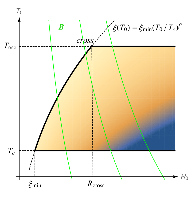
Figure 3: Parameter space of $R_{0}$ and $T_{0}$. The coloured region represents the allowed ($R_{0},T_{0}$) for the formation of closed domain walls initially. Different colours represent different magnitudes of $f(R_{0},T_{0})$ which decreases from the light yellow part to the deep blue part (gradually away from the correlation length $\xi(T_{0})$). The green lines are the contour lines of $B$, i.e. each line corresponds to the same value of $B$, with $B$ increasing from the left lines to the right.

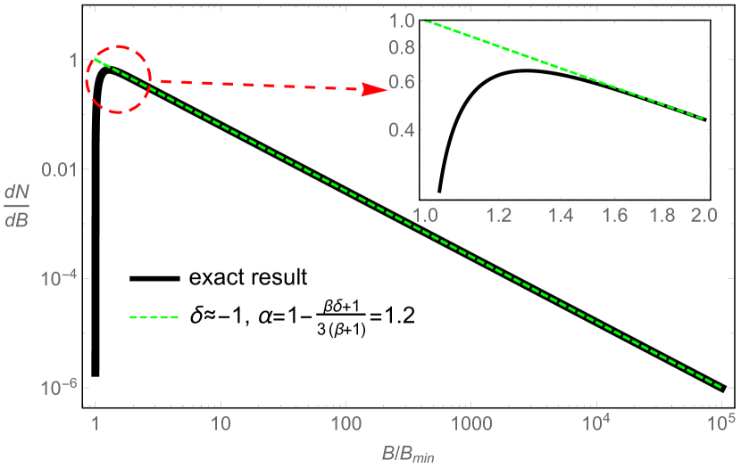
(a)

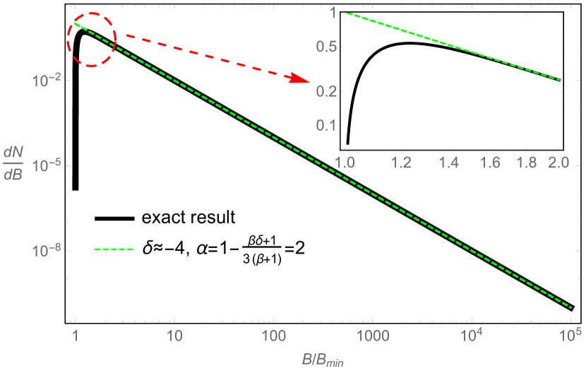
(b)

Figure 4: The relation between $dN/dB$ and $b\equiv B/B_{\rm min}$. We choose $\tau=2$, $\lambda=10$ and $\beta=3.925$ for both subfigures. The difference between (a) and (b) is the values of $\delta$. In (a), $\delta\approx-1$ and thus $\alpha=1.2$; in (b), we choose $\delta\approx-4$ to make $\alpha=2$. The solid black line and dashed green line in each subfigure represents eq. (68) and eq. (71) respectively (the prefactor $N_{0}P/B_{\rm min}$ in the two equations is rescaled to make $dN/dB$ completely shown in the range from 0 to 1 for illustrative purpose).

If we want the upper limit of $T_{0}$ in the integration to be $T_{\rm osc}$, then $B$ has to be larger than $B_{\rm cross}=K\xi^{3}(T_{\rm osc})T_{\rm osc}^{3}$, the value of $B$ at the crossing point where the line $\xi(T_{0})$ intersects the horizontal line $T_{0}=T_{\rm osc}$. We should compare $B_{\rm cross}$ with the minimal baryon charge $B_{\rm min}=K\xi_{\rm min}^{3}T_{c}^{3}$ which corresponds to the closed domain wall initially forming at $T_{0}=T_{c}$ with $R_{0}=\xi_{\rm min}$. We get

$$B_{\rm cross}=\left(\frac{T_{\rm osc}}{T_{c}}\right)^{3(\beta+1)}B_{\rm min}\simeq 10^{15}B_{\rm min}$$ (65)

where we approximate it using $T_{\rm osc}/T_{c}\simeq 10$ and $\beta\simeq 3.925$. We see that the range is $15$ orders of magnitude wide, which is large enough for us to match the baryon charge distribution of nuggets with the energy distribution of solar nanoflares. Therefore, we choose $T_{0}$ is $T_{\rm upper}=T_{c}\cdot[B/(K\xi_{\rm min}^{3}T_{c}^{3})]^{1/3(\beta+1)}$ as the upper limit in eq. (64).

Next, we are going to calculate eq. (64). Using the definitions $r=R_{0}/\xi_{\rm min}$ and $u=T_{0}/T_{c}$, we rewrite eq. (IV.3) in a more concise way

$$f(r,u)=\frac{1}{\xi_{\rm min}T_{c}}\cdot u^{3\beta(\tau-1)+\beta\delta}\cdot r^{2-3\tau}\cdot{\rm e}^{-\lambda r^{2}u^{-2\beta}}.$$ (66)

Substituting $f(r,u)$ into eq. (64) and using the definition $b=B/B_{\rm min}$, we arrive at

$$N(b) =N_{0}P\cdot T_{c}\xi_{\rm min}\int_{1}^{b^{\frac{1}{3(\beta+1)}}}du\int_{u^{\beta}}^{u^{-1}b^{\frac{1}{3}}}dr~{}f(r,u)$$ (67)

$$=N_{0}P\int_{1}^{b^{\frac{1}{3(\beta+1)}}}du\int_{u^{\beta}}^{u^{-1}b^{\frac{1}{3}}}dr~{}\left[u^{3\beta(\tau-1)+\beta\delta}\right.$$

$$~{}~{}~{}~{}\left.\times r^{2-3\tau}\cdot{\rm e}^{-\lambda r^{2}u^{-2\beta}}\right],$$

from which we further get

$$\frac{dN}{dB} =\frac{1}{B_{\rm min}}\frac{dN}{db}=\frac{N_{0}P}{3B_{\rm min}}\cdot b^{-\tau}$$ (68)

$$~{}~{}~{}~{}\times\int_{1}^{b^{\frac{1}{3(\beta+1)}}}du~{}u^{3(\beta+1)(\tau-1)+\beta\delta}\cdot{\rm e}^{-\lambda b^{\frac{2}{3}}u^{-2(\beta+1)}}.$$

This can be further simplified using

$$~{}~{}~{}~{}\int_{1}^{b^{\frac{1}{3(\beta+1)}}}dt~{}u^{m}{\rm e}^{-\lambda b^{2/3}u^{-n}}$$ (69)

$$=\frac{1}{n}(\lambda b^{2/3})^{\frac{1+m}{n}}\cdot\left.\Gamma(-\frac{1+m}{n},\lambda b^{\frac{2}{3}}u^{-n})\right|_{u=1}^{u=b^{\frac{1}{3(\beta+1)}}}$$

$$\simeq\frac{1}{n}(\lambda b^{2/3})^{\frac{1+m}{n}}\cdot\Gamma(-\frac{1+m}{n},\lambda),~{}{\rm for}~{}b\gg 1,$$

where $m\equiv 3(\beta+1)(\tau-1)+\beta\delta$ and $n\equiv 2(\beta+1)$; $\Gamma(s,x)=\int_{x}^{\infty}t^{s-1}{\rm e}^{-t}dt$ is the incomplete gamma function. To obtain the last approximate equality, we neglect the term $\Gamma(-\frac{1+m}{n},\lambda b^{2/3})$ since it is far smaller than the term $\Gamma(-\frac{1+m}{n},\lambda)$ for $b\gg 1$. The condition $b\gg 1$ is satisfied in a wide range of $B$ which is generally several orders larger than $B_{\rm min}$. Substituting (69) into (68), we arrive at

$$\frac{dN}{dB}=\frac{N_{0}P}{3B_{\rm min}}\frac{1}{n}\lambda^{\frac{1+m}{n}}\Gamma(-\frac{1+m}{n},\lambda)\cdot b^{-1+\frac{\beta\delta+1}{3(\beta+1)}},~{}~{}b\gg 1.$$ (70)

We see that $dN/dB$ follows a power-law distribution

$$\frac{dN}{dB}\propto b^{-\alpha},~{}{\rm with}~{}\alpha=1-\frac{\beta\delta+1}{3(\beta+1)},~{}b\gg 1$$ (71)

which verifies the relation (26). The finite-cluster parameters $\tau$ (contained in $m$) and $\lambda$ that we have discussed in section IV.2 only affect the relative magnitude of $dN/dB$, but not the slope of the power-law distribution $-\alpha$.

The parameter $\beta$ describing the relation between axion mass and cosmological temperature is well calculated [54] (see also Appendix A for more details). The other parameter $\delta$ from the model of $T_{0}$ distribution eq. (22) is relatively adjustable, which can result in different slopes of the power-law distribution $dN/dB$. This parameter which may have any sign, plus or minus, describes the distribution of the bubble formation. As we explained in the text, the positive sign of $\delta$ corresponds to the preference of the bubble formation close to $T_{\rm osc}$, while the negative $\delta$ corresponds to a preferred bubble formation close to $T_{c}$ with much stronger tilt of the axion potential.

We plot the baryon charge distribution of nuggets in Fig. 4. We choose $\tau=2$, $\lambda=10$ and $\beta=3.925$ for both subfigures. The difference between them is the value of $\delta$ which is highly underdetermined. In Fig. 4a, we choose $\delta\approx-1$ to make $\alpha=1.2$. The solid black line is the plot of eq. (68), which represents the exact result of the distribution. As a comparison, we also plot the approximate relation (71) represented by the dashed green line, which is straight in the $\log$-$\log$ scale. We see that the approximate relation (71) matches the exact result eq. (68) pretty well after the turning point where the condition $b\gg 1$ becomes valid. In Fig. 4b, we consider the case $\delta\approx-4$ which corresponds to $\alpha=2$. All other ingredients are the same as the first subfigure.

Appendix C On the estimate of parameter $\kappa(T)$ during pre-BBN evolution

The main goal of this Appendix is to make an order of magnitude estimate of the parameter $\kappa(T)$ which is an important element of our analysis in Sect. VI. In simple quantum mechanics terms the parameter $\kappa(T)$ is defined as the transmission coefficient for the baryon to enter and annihilate inside the nugget, while the reflection coefficient $[1-\kappa(T)]$ describes the probability for the baryon’s reflection off the sharp surface of the nugget. One should emphasize that the system cannot be formulated in the simple terms normally used for a one particle QM description. Instead, a proper study of this phenomenon would require a non-perturbative QFT description as many body effects play a crucial role in the computations. This is because the key element of the analysis must be a description of physics at the interface between hadronic phase (as the proton’s wave function is formulated in terms of the quarks) and a CS phase characterized by diquark vacuum condensate. One should emphasize that the diquark condensate is not a local object, but a complicated coherent superposition of quarks similar to Cooper pair in conventional superconductors.

In spite of the complicated annihilation pattern of a baryon in the hadronic phase with diquarks in the CS phase as highlighted above one can easily carry out a simple, order of magnitude, estimate demonstrating that $\kappa(T)\ll 1$, which is precisely the main goal of this Appendix. To simplify things we separate the suppression factor $\kappa$ in two pieces: $\kappa\sim\kappa_{1}\cdot\kappa_{2}$, where $\kappa_{1}$ is defined as the dynamical suppression factor, while $\kappa_{2}$ is defined as the kinematical suppression factor, see below.

The dynamical suppression factor $\kappa_{1}$ can be easily understood from the internal structure of the axion domain wall represented by heavy $\eta^{\prime}$ field which accompanies the axion field in the AQN construction. The corresponding very sharp QCD structure has a width $\sim m^{-1}_{\eta^{\prime}}\ll\Lambda_{\rm QCD}^{-1}$, see [62]. Therefore, one should expect some suppression due to a sharp potential

$$\kappa_{1}(T)\sim\left(\frac{E}{\Lambda_{\rm QCD}}\right)^{3}\sim\left(\frac{T}{\Lambda_{\rm QCD}}\right)^{3},$$ (72)

where we assume that a typical energy $E$ of the incoming three quarks making the proton is order of $T$, while typical strength of the “potential” is order of $\Lambda_{\rm QCD}$. We emphasize that we should formulate the problem in terms of quarks (rather than in terms of a single proton’s wave function) because the annihilation pattern should include 3 antiquarks from a different CS phase. The suppression parameter $\kappa_{1}(T)$ represents the probability for simultaneous transmission of 3 quarks. We note that the factor $E/\Lambda_{\rm QCD}\ll 1$ in (72) for a sharp surface is a very generic QM feature, which is not even sensitive to the sign of interaction. It can be checked with a simple QM problem of scattering of a low energetic particle with $E\rightarrow 0$ on a $\delta(x)$ potential.

There is another suppression factor $\kappa_{2}(T)$ related to a strong mismatch between wave functions of quarks in hadronic phase and antiquarks in CS phase. The corresponding suppression always has a factor $1/N!$ for $N$ constituents which is $N=3$ for proton. The $\kappa_{2}(T)$ also depends on overlapping features of the wave functions from drastically different phases (hadronic vs CS phase). Therefore, we can represent $\kappa_{2}(T)$ as follows

$$\kappa_{2}(T)\sim\frac{1}{N!}\cdot({\rm overlapping~{}integrals}).$$ (73)

Collecting estimates (72) and (73) together one should expect that

$$\kappa(T)\lesssim 10^{-3}~{}{\rm for}~{}T\simeq 40~{}{\rm MeV},\Lambda_{\rm QCD}\simeq 170~{}{\rm MeV},~{}~{}~{}~{}$$ (74)

which represents our final estimate for suppression factor $\kappa(T)$ used in Sect. VI. The order of magnitude estimate (74) is sufficient for qualitative arguments suggesting that the nuggets easily survive the dense and hot environment after the formation.

It is interesting to note that the solitons and anti-solitons (which can be represented as coherent superposition of large $N\rightarrow\infty$ number of constituents) in condensed matter physics do not normally annihilate, but rather experience an elastic scattering, which can be thought as the manifestation of the factor $1/N!$ in (73). It is also known that the anti-proton does not easily annihilate with a large nuclei (considered to be in a nuclear matter phase), but could have a life time as long as $\sim 20~{}{\rm fm}/c$ instead of conventional $\sim{\rm fm}/c$ scale [63]. This suppression of annihilation can be attributed (analogous) to our “overlapping” factor in (73).

Appendix D The AQNs in corona: the turbulence and effective cross section with plasma

The main goal of this Appendix is to explain the crucial difference between our analysis presented in sections V, VI and VII where we argued that very few annihilation events may occur in early Universe. At the same time, it has been argued in [5, 28, 6] that the nuggets of all sizes will experience the complete annihilation in the solar corona when the AQNs enter the solar atmosphere. There is no contradiction between these two claims.

Indeed, our estimates (29) and (VII) indicate that $\Delta B\ll B$ during the entire evolution of the Universe from soon after the nugget’s formation at $T\approx 40$ MeV until the present time. We considered two different regimes: during the hottest period of evolution with $T_{*}<T<40$ MeV then the nuggets’ electrosphere is made of positrons and the annihilation of a baryon charge is highly unlikely and when the temperature drops to below $T_{*}\approx 20$ keV and the electrosphere contains a significant number of protons and baryon charge annihilation may occur as estimated in section VII.

This number of collisions in plasma at $T_{*}\approx 20$ keV should be compared with number of collisions when an AQN enters the solar corona. The corresponding estimate goes as follows, see [5, 28, 6] for the details. First, we estimate the ionized charge of the nugget in terms of the internal temperature $T_{I}$ similar to our estimate (32)

$$Q\simeq 4\pi R^{2}\int^{\infty}_{z_{0}}n(z)dz\sim\frac{4\pi R^{2}}{2\pi\alpha}\cdot\left(T_{I}\sqrt{2m_{e}T_{I}}\right).~{}~{}~{}~{}~{}$$ (75)

Where $T_{P}$ is the temperature of the surrounding plasma. The difference between $T_{P}$ and $T_{I}$ is enormous as emphasized in [6] and related to the fact the nugget propagates in the solar corona with velocity $v\gtrsim 600$ km/s (escape velocity for the Sun) which greatly exceeds the speed of sound $c_{s}$ in corona, i.e. the Mach number $M\equiv v/c_{s}\sim 10$. It is well known that a moving body with such a large Mach number will inevitably generate the shock waves. It is also known that a shock wave generates a discontinuity in temperature, which for large Mach numbers $M\gg 1$ can be approximated as follows

$$\frac{T_{2}}{T_{1}}\simeq M^{2}\cdot\frac{2\gamma(\gamma-1)}{(\gamma+1)^{2}},~{}~{}~{}\gamma\simeq 5/3,$$ (76)

where the temperature $T_{1}\simeq T_{P}$ is identified with the temperature of the surrounding unperturbed plasma, while the high temperature $T_{2}$ can be thought of as the internal temperature of the nuggets $T_{I}$. Precisely this very high internal temperature $T_{I}/T_{P}\sim M^{2}$ being developed due to the shock wave makes a huge difference in comparison with the analysis in section VII for the plasma in the thermal equilibrium at $T\simeq T_{*}$.

The effective cross section of AQN with surrounding protons can be estimated as $\pi R_{\rm eff}^{2}$, where $R_{\rm eff}$ corresponds to the distances where protons from plasma with energy $\sim T_{P}$ can be captured by the nugget

$$T_{P}\sim\frac{Q\alpha}{R_{\rm eff}}.$$ (77)

Combining (75) with (77) one can estimate the enhancement of the effective cross section in comparison with naive estimate $\pi R^{2}$ as follows

$$\left(\frac{R_{\rm eff}}{R}\right)^{2}\simeq\frac{8(m_{e}T_{P})R^{2}}{\pi}\left(\frac{T_{I}}{T_{P}}\right)^{3}\sim M^{6}.$$ (78)

This enhancement factor, of course, is different for different nugget’s velocities as Mach number $M$ varies with $v$. This enhancement factor obviously also changes with time and solar altitude as a result of a motion with the friction and radiation. One should also emphasize that there will be very efficient energy and momentum exchange and heat transfer to the surrounding plasma as a result of nonequilibrium dynamics in the form of the developed turbulence in vicinity of the shock wave front. It should be contrasted with analysis in Section VII when the system is in perfect thermal equilibrium. The numerical simulations performed in [6] suggest that most of the nuggets loose their entire baryon charges due to the annihilation $\Delta B\simeq B$ in vicinity of the transition region at the altitude $\sim 2000$ km where it is known that the drastic changes in temperature and pressure do occur.

From AQN perspective such unusual features of the transition regions as well as the “solar corona heating puzzle” are understood in terms of the dark matter nuggets which continuously hit the solar atmosphere with the flux which has correct magnitude to saturate the EUV and soft x-ray radiation from the corona.

References

- Zhitnitsky [2003] A. R. Zhitnitsky, JCAP 0310, 010 (2003), arXiv:hep-ph/0202161 [hep-ph] .
- Witten [1984] E. Witten, Phys. Rev. D30, 272 (1984).
- Madsen [1999] J. Madsen, Hadrons in dense matter and hadrosynthesis. Proceedings, 11th Chris Engelbrecht Summer School, Cape Town, South Africa, February 4-13, 1998, Lect. Notes Phys. 516, 162 (1999), [,162(1998)], arXiv:astro-ph/9809032 [astro-ph] .
- Flambaum and Zhitnitsky [2019] V. V. Flambaum and A. R. Zhitnitsky, Phys. Rev. D99, 023517 (2019), arXiv:1811.01965 [hep-ph] .
- Zhitnitsky [2017] A. Zhitnitsky, JCAP 1710, 050 (2017), arXiv:1707.03400 [astro-ph.SR] .
- Raza et al. [2018] N. Raza, L. van Waerbeke, and A. Zhitnitsky, Phys. Rev. D98, 103527 (2018), arXiv:1805.01897 [astro-ph.SR] .
- Liang and Zhitnitsky [2016] X. Liang and A. Zhitnitsky, Phys. Rev. D94, 083502 (2016), arXiv:1606.00435 [hep-ph] .
- Ge et al. [2017] S. Ge, X. Liang, and A. Zhitnitsky, Phys. Rev. D96, 063514 (2017), arXiv:1702.04354 [hep-ph] .
- Ge et al. [2018] S. Ge, X. Liang, and A. Zhitnitsky, Phys. Rev. D97, 043008 (2018), arXiv:1711.06271 [hep-ph] .
- Bowman et al. [2018] J. D. Bowman, A. E. E. Rogers, R. A. Monsalve, T. J. Mozdzen, and N. Mahesh, Nature 555, 67 (2018), arXiv:1810.05912 [astro-ph.CO] .
- Feng and Holder [2018] C. Feng and G. Holder, Astrophys. J. 858, L17 (2018), arXiv:1802.07432 [astro-ph.CO] .
- Lawson and Zhitnitsky [2019] K. Lawson and A. Zhitnitsky, Phys. Dark Univ 24, 100295 (2019), arXiv:1804.07340 [hep-ph] .
- Lawson [2011] K. Lawson, Phys. Rev. D83, 103520 (2011), arXiv:1011.3288 [astro-ph.HE] .
- Aartsen et al. [2014] M. G. Aartsen et al. (IceCube), Eur. Phys. J. C74, 2938 (2014), arXiv:1402.3460 [astro-ph.CO] .
- Gorham [2012] P. Gorham, Phys. Rev. D86, 123005 (2012), arXiv:1208.3697 [astro-ph.CO] .
- Jacobs et al. [2015] D. M. Jacobs, G. D. Starkman, and B. W. Lynn, Mon. Not. Roy. Astron. Soc. 450, 3418 (2015), arXiv:1410.2236 [astro-ph.CO] .
- Gorham and Rotter [2017] P. Gorham and B. J. Rotter, Phys. Rev. D95, 103002 (2017), arXiv:1507.03545 [astro-ph.CO] .
- Lawson and Zhitnitsky [2017] K. Lawson and A. Zhitnitsky, Phys. Rev. D95, 063521 (2017), arXiv:1510.07646 [astro-ph.HE] .
- Prantzos et al. [2011] N. Prantzos et al., Rev. Mod. Phys. 83, 1001 (2011), arXiv:1009.4620 [astro-ph.HE] .
- Oaknin and Zhitnitsky [2005] D. H. Oaknin and A. R. Zhitnitsky, Phys. Rev. Lett. 94, 101301 (2005), arXiv:hep-ph/0406146 [hep-ph] .
- Zhitnitsky [2007] A. Zhitnitsky, Phys. Rev. D76, 103518 (2007), arXiv:astro-ph/0607361 [astro-ph] .
- Forbes and Zhitnitsky [2008a] M. M. Forbes and A. R. Zhitnitsky, JCAP 0801, 023 (2008a), arXiv:astro-ph/0611506 [astro-ph] .
- Lawson and Zhitnitsky [2008] K. Lawson and A. R. Zhitnitsky, JCAP 0801, 022 (2008), arXiv:0704.3064 [astro-ph] .
- Forbes and Zhitnitsky [2008b] M. M. Forbes and A. R. Zhitnitsky, Phys. Rev. D78, 083505 (2008b), arXiv:0802.3830 [astro-ph] .
- Forbes et al. [2010] M. M. Forbes, K. Lawson, and A. R. Zhitnitsky, Phys. Rev. D82, 083510 (2010), arXiv:0910.4541 [astro-ph.GA] .
- Lawson and Zhitnitsky [2013a] K. Lawson and A. R. Zhitnitsky, Phys. Lett. B724, 17 (2013a), arXiv:1210.2400 [astro-ph.CO] .
- Lawson and Zhitnitsky [2013b] K. Lawson and A. R. Zhitnitsky, in Cosmic Frontier Workshop: Snowmass 2013 Menlo Park, USA, March 6-8, 2013 (2013) arXiv:1305.6318 [astro-ph.CO] .
- Zhitnitsky [2018] A. Zhitnitsky, Phys. Dark Univ. 22, 1 (2018), arXiv:1801.01509 [astro-ph.SR] .
- Mitra-Kraev and Benz [2001] U. Mitra-Kraev and A. O. Benz, Astronomy & Astrophysics 373, 318 (2001).
- Pauluhn and Solanki [2007] A. Pauluhn and S. K. Solanki, Astron. Astrophys. 462, 311 (2007), arXiv:astro-ph/0612585 [astro-ph] .
- Bingert, S. and Peter, H. [2013] Bingert, S. and Peter, H., A&A 550, A30 (2013).
- Sikivie [1982] P. Sikivie, Physical Review Letters 48, 1156 (1982).
- Vilenkin and Everett [1982] A. Vilenkin and A. E. Everett, Physical Review Letters 48, 1867 (1982).
- Preskill et al. [1983] J. Preskill, M. B. Wise, and F. Wilczek, Phys. Lett. B120, 127 (1983), [,URL(1982)].
- Abbott and Sikivie [1983] L. F. Abbott and P. Sikivie, Phys. Lett. B120, 133 (1983), [,URL(1982)].
- Dine and Fischler [1983] M. Dine and W. Fischler, Phys. Lett. B120, 137 (1983), [,URL(1982)].
- Chang et al. [1999] S. Chang, C. Hagmann, and P. Sikivie, Phys. Rev. D59, 023505 (1999), arXiv:hep-ph/9807374 [hep-ph] .
- Hiramatsu et al. [2012] T. Hiramatsu, M. Kawasaki, K. Saikawa, and T. Sekiguchi, Phys. Rev. D85, 105020 (2012), [Erratum: Phys. Rev.D86,089902(2012)], arXiv:1202.5851 [hep-ph] .
- Kawasaki et al. [2015] M. Kawasaki, K. Saikawa, and T. Sekiguchi, Phys. Rev. D91, 065014 (2015), arXiv:1412.0789 [hep-ph] .
- Fleury and Moore [2016] L. Fleury and G. D. Moore, JCAP 1601, 004 (2016), arXiv:1509.00026 [hep-ph] .
- Klaer and Moore [2017] V. B. Klaer and G. D. Moore, JCAP 1711, 049 (2017), arXiv:1708.07521 [hep-ph] .
- Gorghetto et al. [2018] M. Gorghetto, E. Hardy, and G. Villadoro, JHEP 07, 151 (2018), arXiv:1806.04677 [hep-ph] .
- Witten [1980] E. Witten, Annals Phys. 128, 363 (1980).
- Witten [1998] E. Witten, Phys. Rev. Lett. 81, 2862 (1998), arXiv:hep-th/9807109 [hep-th] .
- Vachaspati and Vilenkin [1984] T. Vachaspati and A. Vilenkin, Physical Review D 30, 2036 (1984).
- Stauffer [1979] D. Stauffer, Physics Reports 54, 1 (1979).
- Stauffer and Aharony [2014] D. Stauffer and A. Aharony, Introduction to percolation theory: revised second edition (CRC press, 2014).
- Bauchspiess and Stauffer [1978] K. Bauchspiess and D. Stauffer, Journal of Aerosol Science 9, 567 (1978).
- Isichenko [1992] M. B. Isichenko, Reviews of modern physics 64, 961 (1992).
- Grinchuk [2002] P. Grinchuk, Physical Review E 66, 016124 (2002).
- Lubensky and McKane [1981] T. Lubensky and A. McKane, Journal of Physics A: Mathematical and General 14, L157 (1981).
- Wantz and Shellard [2010a] O. Wantz and E. P. S. Shellard, Nucl. Phys. B829, 110 (2010a), arXiv:0908.0324 [hep-ph] .
- Wantz and Shellard [2010b] O. Wantz and E. P. S. Shellard, Phys. Rev. D82, 123508 (2010b), arXiv:0910.1066 [astro-ph.CO] .
- Borsanyi et al. [2016] S. Borsanyi et al., Nature 539, 69 (2016), arXiv:1606.07494 [hep-lat] .
- Vachaspati [2017] T. Vachaspati, arXiv preprint arXiv:1706.03868 (2017).
- Yoshida et al. [2006] N. Yoshida, K. Omukai, L. Hernquist, and T. Abel, Proceedings, 10th International Conference on B-Physics at Hadron Machines (Beauty 2005): Assisi (Perugia), Italy, 20-24 June 2005, Astrophys. J. 652, 6 (2006), arXiv:astro-ph/0606106 [astro-ph] .
- Fischer et al. [2018] H. Fischer, X. Liang, Y. Semertzidis, A. Zhitnitsky, and K. Zioutas, Phys. Rev. D98, 043013 (2018), arXiv:1805.05184 [hep-ph] .
- Liang and Zhitnitsky [2019] X. Liang and A. Zhitnitsky, Phys. Rev. D99, 023015 (2019), arXiv:1810.00673 [hep-ph] .
- Lawson et al. [2019] K. Lawson, X. Liang, A. Mead, M. S. R. Siddiqui, L. Van Waerbeke, and A. Zhitnitsky, (2019), arXiv:1905.00022 [astro-ph.CO] .
- Baumann [2014] D. Baumann, University lecture notes (2014).
- Petzold [1981] L. R. Petzold, SIAM Journal on Numerical Analysis 18, 455 (1981).
- Forbes and Zhitnitsky [2001] M. M. Forbes and A. R. Zhitnitsky, JHEP 10, 013 (2001), arXiv:hep-ph/0008315 [hep-ph] .
- Mishustin et al. [2005] I. N. Mishustin, L. M. Satarov, T. J. Burvenich, H. Stoecker, and W. Greiner, Phys. Rev. C71, 035201 (2005), arXiv:nucl-th/0404026 [nucl-th] .