Flexible Clustering with a Sparse Mixture of Generalized Hyperbolic Distributions

Abstract

Robust clustering of high-dimensional data is an important topic because, in many practical situations, real data sets are heavy-tailed and/or asymmetric. Moreover, traditional model-based clustering often fails for high dimensional data due to the number of free covariance parameters. A parametrization of the component scale matrices for the mixture of generalized hyperbolic distributions is proposed by including a penalty term in the likelihood constraining the parameters resulting in a flexible model for high dimensional data and a meaningful interpretation. An analytically feasible EM algorithm is developed by placing a gamma-Lasso penalty constraining the concentration matrix. The proposed methodology is investigated through simulation studies and two real data sets.

Keywords: Asymmetric data, Flexible clustering, Generalized hyperbolic distributions, Penalized likelihood, Sparse mixture models

1 Introduction

In recent years, the use of finite mixture distributions to model heterogeneous data has undergone intensive development in numerous fields such as pattern recognition, cluster analysis, and bioinformatics. Gaussian mixture models dominate the literature in the past century. However when clusters are asymmetric and/or have heavier tails, Gaussian mixture models tend to overestimate the number of clusters. Ultimately, this leads to incorrect clustering results. Consider the data in Fig. 1, where there are two asymmetric clusters, are generated from a $G=2$ component generalized hyperbolic distributions (MGHD; Browne and McNicholas, 2015). Gaussian mixtures are fitted to these data for $G=1,\ldots,6$ components and the Bayesian Information criterion (BIC; Schwarz, 1978) selects a $G=3$ component model. Moreover, the Gaussian components cannot be merged to return the correct clusters: the green component has been used to capture all points that do not fit within one of the other two components (Fig. 1). Therefore, recent work on model-based clustering has focused on mixture of non-elliptical distributions (e.g., Karlis and Santourian, 2009; Lin, 2010). Recent reviews of model-based clustering are given by Bouveyron and Brunet-Saumard (2014) and McNicholas (2016b).

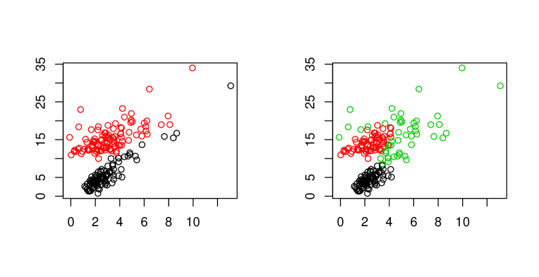
Figure 1: Scatter plots of a two-component mixture of GHD distribution (left) and the classification from a $G=3$ component Gaussian mixture (right).

The former review focuses on high-dimensional data while the later is more general but devotes quite some space to methods for high-dimensional data. This is reflective of the quite substantial body of literature that has already been devoted to high-dimensional data.

Although mixtures of Gaussian distributions had been used almost exclusively until the turn of the century, it is now quite common to use approaches that relax this assumption. In the case of high dimensional data, model-based clustering and classification methods that allow for asymmetric and/or heavier tailed clusters often fail due to the number of free covariance parameters and, therefore, alternative techniques need to be developed. One such technique is to map the data to a (much) lower dimensional space. The mixture of factor analyzers models with non-elliptical distributions took became popular recently, including work on multivariate skew-t distributions (Murray et al., 2014a, b) and generalized hyperbolic distributions (Tortora et al., 2016). Each of these methods works well with particular types of data sets; however, the GHD represents perhaps the most flexible among the recent series of alternatives to the Gaussian component density. A parameterization of the component covariance matrices $\bm{\Sigma}_{1},\ldots,\bm{\Sigma}_{G}$ has also been considered for dimensionality reduction of Gaussian mixture models (e.g., Celeux and Govaert, 1995; Bouveyron et al., 2007). Krishnamurthy (2011) presents a method which considers a sparse covariance matrix for Gaussian mixture models. This is achieved by including a penalty term in the likelihood constraining the parameters.

Herein, we present an extension of the work done by Krishnamurthy (2011) by considering a mixture of generalized hyperbolic distributions. The method in Krishnamurthy (2011) also involves a Laplace prior on each element of the concentration matrix (inverse of the covariance matrix). We extend this herein by considering placing a gamma hyperprior on the hyperparameter. In Sect. 2 we give a detailed background, Sect. 3 gives a detailed description of the method, Sect. LABEL:sec:NE looks at simulations and data analyses, and we end with a discussion (Sect. 6).

2 Background

2.1 Model-Based Clustering

One common method for clustering is model-based clustering which makes use of a finite mixture model. A $G$ component finite mixture model assumes a random vector $\mathbf{X}$ has density

$$f(\mathbf{x}~{}|~{}{\bm{\vartheta}})=\sum_{g=1}^{G}\pi_{g}f_{g}(\mathbf{x}~{}|~{}{\bm{\theta}}_{g}),$$

where ${\bm{\vartheta}}=\left(\pi_{1},\pi_{2},\ldots,\pi_{G},{\bm{\theta}}_{1},{\bm{\theta}}_{2},\ldots,{\bm{\theta}}_{G}\right)$, $f_{g}(\cdot)$ is the $g$th component density, and $\pi_{g}>0$ is the $g$th mixing proportion such that $\sum_{i=1}^{G}\pi_{g}=1$. McNicholas (2016) traces the relationship between clustering and mixture models all the way back to Tiedeman (1955) with the earliest use a mixture model for clustering presented in Wolfe (1965) who used a Gaussian mixture model. Other early work in the area of Gaussian mixture models can be found in Baum et al. (1970) and Scott and Symons (1971).

The mathematical tractability of the Gaussian mixture model has made it very popular in the literature, however; a Gaussian distribution may not be appropriate in the presence of asymmetry or outliers. To combat this issue work in the area of non-Gaussian mixtures has become popular including distributions with parameterization for concentration such as the $t$ distribution (Peel and McLachlan, 2000; Andrews and McNicholas, 2011, 2012; Lin et al., 2014) and the power exponential distribution (Dang et al., 2015). There has also been recent work in the area of skewed distributions such as the skew-$t$ distribution, (Lin, 2010; Vrbik and McNicholas, 2012, 2014; Lee and McLachlan, 2014; Murray et al., 2014b, a) and the generalized hyperbolic distribution, Browne and McNicholas (2015).

Although model-based clustering with the aforementioned distributions have been shown to exhibit good performance for lower dimensional datasets, they generally fail due to the number of free covariance parameters being quadratic in the dimension. Therefore, for higher dimensional datasets, the model is essentially overfitted which can lead to multiple possibilities for assignments of observations to clusters ultimately resulting in poor classification performance.

2.2 Sparse Gaussian Mixture Models

The work presented herein extends the work by Krishnamurthy (2011) in which the author proposed using a sparse Gaussian mixture model to model high dimensional data. The model assumed a random sample $\mathbf{X}_{i}$, $i=1\ldots,n$ came from a $p$ dimensional Gaussian population with $G$ subpopulations with means $\mbox{\boldmath$\mu$}_{g}$ and covariances $\mathbf{\Sigma}_{g}$. The penalized observed data log-likelihood utilized for this model is of the form

$$\mathcal{L}({\bm{\vartheta}})=\sum_{i=1}^{n}\log\left(\sum_{g=1}^{G}\pi_{g}\phi({\bm{\theta}}_{g})\right)+\sum_{g=1}^{G}\log\mathbf{C}_{g},$$

where $\mathbf{C}_{g}=\mathbf{\Sigma}_{g}^{-1}$ is the concentration matrix for component $g$ and $\phi(\cdot)$ denotes the multivariate Gaussian density.

If it is assumed that $C_{gij}\sim\text{Laplace}(0,\lambda)$, then the penalty term becomes $\sum_{g=1}^{G}\lambda||\mathbf{C}_{g}||_{1}$, where $||\cdot||_{1}$ is the sum of the absolute values of the entries of $\mathbf{C}_{g}$.

Parameter estimation for this model requires the use of the graphical lasso method, (Friedman et al., 2008) in conjunction with an expectation maximization algorithm, Dempster et al. (1977). The graphical lasso is a method for the maximization of

$$f(\mathbf{C})=\log\det(\mathbf{C})-\,\mbox{tr}(\mathbf{S}\mathbf{C})-\rho||\mathbf{C}||_{1},$$

where $\mathbf{S}$ is the empirical covariance matrix and $\rho$ is a tuning parameter. The graphical lasso uses a similar approach Banerjee et al. (2008) who considers the estimation of $\mathbf{\Sigma}$ by optimizing over the rows and columms using a block coordinate descent approach.

2.3 Generalized Hyperbolic Distribution

Before introducing the generalized hyperbolic distribution, we briefly discuss the generalized inverse Gaussian distribution. A random variable $Y$ follows a generalized inverse gaussian distribution, denoted by $\text{GIG}(e,h,\gamma)$, if its density function can be written as

$$f(y|e,h,\gamma)=\frac{\left({e}/{h}\right)^{\frac{\gamma}{2}}y^{\gamma-1}}{2K_{\gamma}(\sqrt{eh})}\exp\left\{-\frac{ey+{h}/{y}}{2}\right\},$$

where $e,h>0$ and

$$K_{\gamma}(u)=\frac{1}{2}\int_{0}^{\infty}y^{\gamma-1}\exp\left\{-\frac{u}{2}\left(y+\frac{1}{y}\right)\right\}dy$$

is the modified Bessel function of the third kind with index $\gamma\in\mathbb{R}$. Expectations of some functions of a GIG random variable have a mathematically tractable form, e.g.:

$$\mathbb{E}(Y)=\sqrt{\frac{h}{e}}\frac{K_{\gamma+1}(\sqrt{eh})}{K_{\gamma}(\sqrt{eh})},$$ (1)

$$\mathbb{E}\left({1}/{Y}\right)=\sqrt{\frac{e}{h}}\frac{K_{\gamma+1}(\sqrt{eh})}{K_{\gamma}(\sqrt{eh})}-\frac{2\gamma}{h},$$ (2)

$$\mathbb{E}(\log Y)=\log\left(\sqrt{\frac{h}{e}}\right)+\frac{1}{K_{\gamma}(\sqrt{eh})}\frac{\partial}{\partial\gamma}K_{\gamma}(\sqrt{eh}).$$ (3)

Although these expectations will be useful for parameter estimation, the derivation of the generalized hyperbolic distribution, as parameterized in Browne and McNicholas (2015), relies on parameterization with density

$$g(y|\omega,\eta,\gamma)=\frac{\left({w}/{\eta}\right)^{\gamma-1}}{2\eta K_{\gamma}(\omega)}\exp\left\{-\frac{\omega}{2}\left(\frac{w}{\eta}+\frac{\eta}{w}\right)\right\},$$ (4)

where $\omega=\sqrt{eh}$ and $\eta=\sqrt{e/h}$. For notational clarity, we will denote the parameterization given in (4) by $\text{I}(\omega,\eta,\gamma)$.

Specifically the generalized hyperbolic distribution, as parameterized in Browne and McNicholas (2015), arises as a special case of a variance-mean mixture model. This assumes that the $p$-dimensional random vector $\mathbf{X}$ can be written as

$$\mathbf{X}=\mbox{\boldmath$\mu$}+W\bm{\alpha}+\sqrt{W}\mathbf{U},$$

where $\mu$ is a location parameter, $\bm{\alpha}$ is the skewness, $\mathbf{U}\sim\mathcal{N}({\bf 0},\mathbf{\Sigma})$ and $W\sim\text{I}(\omega,1,\gamma)$. The resulting density of the generalized hyperbolic distribution is

$$\begin{split}f_{\text{GH}}(\mathbf{x}|{\bm{\theta}})&=\exp\left\{(\mathbf{x}-\mbox{\boldmath$\mu$})^{\prime}\mathbf{\Sigma}^{-1}\bm{\alpha}\right\}\left[\frac{\omega+\delta(\mathbf{x},\mbox{\boldmath$\mu$};\mathbf{\Sigma})}{\omega+\bm{\alpha}^{\prime}\mathbf{\Sigma}^{-1}\bm{\alpha}}\right]^{\frac{\gamma-p/2}{2}}\\ &\times\frac{K_{\gamma-p/2}(\sqrt{[\omega+\bm{\alpha}^{\prime}\mathbf{\Sigma}^{-1}\bm{\alpha}][\omega+\delta(\mathbf{x},\mbox{\boldmath$\mu$};\mathbf{\Sigma})]})}{(2\pi)^{p/2}|\mathbf{\Sigma}|^{1/2}K_{\gamma}(\omega)},\\ \end{split}$$

where $\lambda\in\mathbb{R}$ is an index parameter, $\omega>0$ is a concentration parameter and

$$\delta(\mathbf{x},\mbox{\boldmath$\mu$};\mathbf{\Sigma})=(\mathbf{x}-\mbox{\boldmath$\mu$})^{\prime}\mathbf{\Sigma}^{-1}(\mathbf{x}-\mbox{\boldmath$\mu$}).$$

3 Methodology

3.1 Overview

Extending the methodology in Krishnamurthy (2011) it is assumed that for each group $g$, $\lambda_{g}\sim\text{Gamma}(s,r)$ and if $\mathbf{C}_{g}$ is the inverse of some scale matrix $\mathbf{\Sigma}_{g}$, then $C_{gij}|\lambda_{g}\sim\text{Laplace}(0,\lambda_{g})$. The joint density of $\mathbf{C}_{g}$ and $\lambda_{g}$ is then

$$\begin{split}f(\mathbf{c}_{g},\lambda_{g})&=\frac{r^{s}}{\Gamma(s)}\lambda_{g}^{s-1}\exp\left\{-r\lambda_{g}\right\}\prod_{i=1}^{p}\prod_{j=1}^{p}\frac{\lambda_{g}}{2}\exp\left\{-\lambda_{g}|c_{gij}|\right\}\\ &=\frac{r^{s}}{\Gamma(s)2^{p^{2}}}\lambda_{g}^{s+p^{2}-1}\exp\left\{-\lambda_{g}(r+||\mathbf{c}_{g}||_{1})\right\}.\end{split}$$

It can be shown that

$$\lambda_{g}|\mathbf{c}_{g}\sim\text{gamma}(s+p^{2},r+||\mathbf{c}_{g}||_{1})$$

and the marginal distribution of $\mathbf{C}_{g}$ is

$$f(\mathbf{c}_{g})=\frac{r^{s}}{\Gamma(s)2^{p}}\left[\frac{\Gamma(s+p^{2})}{(r+||\mathbf{c}_{g}||_{1})^{s+p^{2}}}\right].$$

Suppose we observe a random sample $\mathbf{x}_{1},\mathbf{x}_{2},\ldots,\mathbf{x}_{n}$ from generalized hyperbolic distributed population with $G$ underlying subpopulations (groups). Following the methodology in Krishnamurthy (2011), the observed penalized log-likelihood is

$$\mathcal{L}(\mbox{\boldmath$\vartheta$})=\sum_{i=1}^{N}\log\sum_{g=1}^{G}\pi_{g}f_{\text{GH}}(\mathbf{x}_{i}|\mbox{\boldmath$\mu$}_{g},\bm{\alpha}_{g},\mathbf{\Sigma}_{g},\omega_{g},\gamma_{g})+\sum_{g=1}^{G}\log f(\mathbf{c}_{g}).$$

3.2 Parameter Estimation

Introducing the latent variables $w_{ig}$, the group memberships $z_{ig}$ and the unknown $\lambda_{g}$, the complete data penalized log-likelihood is

$$\begin{split}&\mathcal{L}_{C}(\mbox{\boldmath$\vartheta$})=K+\frac{1}{2}\sum_{i=1}^{N}\sum_{g=1}^{G}z_{ig}\log|\mathbf{C}_{g}|+\sum_{i=1}^{N}\sum_{g=1}^{G}z_{ig}\log h(w_{ig}~{}|~{}\omega_{g},\gamma_{g})\\ &-\frac{1}{2}\,\mbox{tr}\bigg{\{}\sum_{g=1}^{G}\mathbf{C}_{g}\sum_{i=1}^{N}z_{ig}[(1/w_{ig})(\mathbf{x}_{i}-\mbox{\boldmath$\mu$}_{g})(\mathbf{x}_{i}-\mbox{\boldmath$\mu$}_{g})^{\prime}-(\mathbf{x}_{i}-\mbox{\boldmath$\mu$}_{g})\bm{\alpha}_{g}^{\prime}-\bm{\alpha}_{g}(\mathbf{x}_{i}-\mbox{\boldmath$\mu$}_{g})^{\prime}+w_{ig}\bm{\alpha}_{g}\bm{\alpha}_{g}^{\prime}]\bigg{\}}\\ &-\sum_{g=1}^{G}\lambda_{g}||\mathbf{C}_{g}||_{1},\end{split}$$

where $K$ is a constant with respect to the parameters. An EM algorithm is used to maximize the complete likelihood and an outline is given below.
E Step: Update $\hat{z}_{ig},a_{ig},b_{ig},c_{ig},\hat{\lambda}_{g}$, where

$$\hat{z}_{ig} :=\mathbb{E}\left[z_{ig}|\mathbf{x}_{i}\right]=\frac{\hat{\pi}_{g}^{(t)}f_{\text{GH}}(\mathbf{X}_{i}~{}|~{}\hat{{\bm{\vartheta}}}^{(t)}_{g})}{\sum_{h=1}^{G}\hat{\pi}_{h}^{(t)}f_{\text{GH}}(\mathbf{X}_{i}~{}|~{}\hat{{\bm{\vartheta}}}^{(t)}_{h})},$$

$$a_{ig} :=\mathbb{E}\left[W_{ig}~{}|~{}\mathbf{x}_{i},z_{ig}=1\right],$$

$$b_{ig} :=\mathbb{E}\left[{1}/{W_{ig}}|\mathbf{x}_{i},z_{ig}=1\right],$$

$$c_{ig} :=\mathbb{E}\left[\log W_{ig}|\mathbf{x}_{i},z_{ig}=1\right],$$

and $\hat{{\bm{\vartheta}}}^{(t)}_{g}=\left\{\hat{\mbox{\boldmath$\mu$}}^{(t)}_{g},\hat{\bm{\alpha}}^{(t)}_{g},\hat{\gamma}_{g}^{(t)},\hat{\omega}_{g}^{(t)},\hat{\mathbf{\Sigma}}_{g}^{(t)}\right\}$. Fortunately, in the generalized hyperbolic case,

$$W_{ig}|\mathbf{x}_{i},z_{ig}=1\sim\text{I}(\omega_{g}+\bm{\alpha}_{g}^{\prime}\mathbf{C}_{g}\bm{\alpha},\omega_{g}+\delta(\mathbf{x}_{i},\mbox{\boldmath$\mu$}_{g}|\mathbf{C}_{g}),\gamma_{g}-p/2),$$

so these expectations can be calculated using (1)–(3).

The update for $\lambda_{g}$ is given by

$$\mathbb{E}\left[\lambda_{g}|\mathbf{c}_{g}\right]=\hat{\lambda}_{g}=\frac{s+p^{2}}{||\hat{\mathbf{c}}_{g}^{(t)}||_{1}+r}.$$

Hereafter we utilise the notation $n_{g}=\sum_{i=1}^{n}\hat{z}_{ig}$, $\bar{a}_{g}=1/n_{g}\sum_{i=1}^{n}\hat{z}_{ig}a_{ig}$, $\bar{b}_{g}=1/n_{g}\sum_{i=1}^{n}\hat{z}_{ig}b_{ig}$ and $\bar{c}_{g}=1/n_{g}$
$\sum_{i=1}^{n}\hat{z}_{ig}c_{ig}$.

M Step: Update $\pi_{g}$, $\mbox{\boldmath$\mu$}_{g}$, $\bm{\alpha}_{g}$, $\omega_{g}$, $\gamma_{g}$ and $\mathbf{C}_{g}$.
The updates for all these parameters, except $\mathbf{C}_{g}$, are identical to those given in Browne and McNicholas (2015) and are given by

$$\begin{split}\hat{\pi}_{g}^{(t+1)}&=\frac{1}{n}\sum_{i=1}^{n}\hat{z}_{ig},\quad\hat{\mbox{\boldmath$\mu$}}^{(t+1)}_{g}=\frac{\sum_{i=1}^{n}\hat{z}_{ig}\mathbf{x}_{i}(\bar{a}_{g}b_{ig}-1)}{\sum_{i=1}^{n}\hat{z}_{ig}(\bar{a}_{g}b_{ig}-1)},\\ \hat{\bm{\alpha}}^{(t+1)}_{g}&=\frac{\sum_{i=1}^{n}\hat{z}_{ig}\mathbf{x}_{i}(\bar{b}_{g}-b_{ig})}{\sum_{i=1}^{n}\hat{z}_{ig}(\bar{a}_{g}b_{ig}-1)}.\end{split}$$

The updates for $\gamma_{g}$ and $\omega_{g}$ cannot be obtained in closed form and have to be updated using numerical techniques. The details are given in Browne and McNicholas (2015) and the resulting updates are

$$\hat{\gamma}_{g}^{(t+1)}=\bar{c}_{g}\hat{\gamma}_{g}^{(t)}\left[\left.\frac{\partial}{\partial s}\log(K_{s}(\hat{\omega}_{g}^{(t)}))\right|_{s=\hat{\gamma}_{g}^{(t)}}\right]^{-1},$$ (5)

$$\hat{\omega}_{g}^{(t+1)}=\hat{\omega}_{g}^{(t)}-\left[\left.\frac{\partial}{\partial s}q(\hat{\gamma}_{g}^{(t+1)},s)\right|_{s=\hat{\omega}_{g}^{(t)}}\right]\left[\left.\frac{\partial^{2}}{\partial s^{2}}q(\hat{\gamma}_{g}^{(t+1)},s)\right|_{s=\hat{\omega}_{g}^{(t)}}\right]^{-1},$$

where the derivative of the Bessel function with respect to the index in (5) is calculated numerically and

$$q(\gamma_{g},\omega_{g})=\sum_{i=1}^{N}z_{ig}\bigg{[}\log(K_{\gamma_{g}}(\omega_{g}))-\gamma_{g}\log w_{ig}-\frac{1}{2}\omega_{g}\left(w_{ig}+\frac{1}{w_{ig}}\right)\bigg{]}.$$

The partials in (3.2) are described in Browne and McNicholas (2015) and can be written

$$\frac{\partial}{\partial\omega_{g}}q(\gamma_{g},\omega_{g})=\frac{1}{2}\left[R_{\gamma_{g}}(\omega_{g})+R_{-\gamma_{g}}(\omega_{g})-(\bar{a}_{g}+\bar{b}_{g})\right],$$

$$\begin{split}\frac{\partial^{2}}{\partial\omega_{g}^{2}}q(\gamma_{g},\omega_{g})=\frac{1}{2}&\left[R_{\gamma_{g}}(\omega_{g})^{2}-\frac{1+2\gamma_{g}}{\omega_{g}}R_{\gamma_{g}}(\omega_{g})-1+R_{-\gamma_{g}}(\omega_{g})^{2}-\frac{1-2\gamma_{g}}{\omega_{g}}R_{-\gamma_{g}}(\omega_{g})-1\right],\end{split}$$

where $R_{\gamma_{g}}(\omega_{g})=K_{\gamma_{g}+1}(\omega_{g})/K_{\gamma_{g}}(\omega_{g})$.

The update for $\mathbf{\Sigma}_{g}$ would be calculated as follows. First find

$$\hat{\mathbf{C}}_{g}^{(t+1)}=\underset{\mathbf{C}}{\arg\min}\left\{-\log|\mathbf{C}|+\,\mbox{tr}(\mathbf{C}{\bf S}_{g})+\frac{\hat{\lambda}_{g}}{n_{g}}||\mathbf{C}||_{1}\right\},$$

where

$$\begin{split}{\bf S}_{g}=\frac{1}{n_{g}}&\bigg{\{}\sum_{i=1}^{N}\hat{z}_{ig}\left[b_{ig}(\mathbf{x}_{i}-\hat{\mbox{\boldmath$\mu$}}_{g}^{(t+1)})(\mathbf{x}_{i}-\hat{\mbox{\boldmath$\mu$}}_{g}^{(t+1)})^{\prime}-(\mathbf{x}_{i}-\hat{\mbox{\boldmath$\mu$}}_{g}^{(t+1)})(\hat{\bm{\alpha}}_{g}^{(t+1)})^{\prime}\right.\\ &\left.-\hat{\bm{\alpha}}_{g}^{(t+1)}(\mathbf{x}_{i}-\hat{\mbox{\boldmath$\mu$}}_{g}^{(t+1)})^{\prime}+a_{ig}\hat{\bm{\alpha}}_{g}^{(t+1)}(\hat{\bm{\alpha}}_{g}^{(t+1)})^{\prime}\right]\bigg{\}},\end{split}$$

using the graphical lasso method . The update for $\mathbf{\Sigma}_{g}$ is then

$$\hat{\mathbf{\Sigma}}_{g}^{(t+1)}=\hat{\mathbf{C}}^{(t+1)^{-1}}_{g}$$

Hereafter, we will refer to this model as the GHD-GLS model.

3.3 Convergence Criterion

It is possible for the likelihood to “plateau" and then increase again thus terminating the algorithm prematurely if lack of progress was used as the convergence criteria. One alternative is to use a criterion based on the Aitken acceleration Aitken (1926). The acceleration at iteration $t$ is

$$a^{(t)}=\frac{l^{(t+1)}-l^{(t)}}{l^{(t)}-l^{(t-1)}},$$

where $l^{(t)}$ is the observed likelihood at iteration $t$. We then define

$$l_{\infty}^{(t+1)}=l^{(t)}+\frac{(l^{(t+1)}-l^{(t)})}{1-a^{(t)}},$$

(refer to Böhning et al. (1994); Lindsay (1995)). This quantity is an estimate of the observed log likelihood after many iterations at iteration $t+1$. As in McNicholas et al. (2010), we terminate the algorithm when $l_{\infty}^{(k+1)}-l^{(k)}<\epsilon$, $\epsilon>0$, provided the difference is positive.

3.4 Model Selection

In a general clustering scenario, the number of groups is not known a priori and therefore have to be selected using some criterion. Because the lasso penalty term shrinks the elements of the concentration matrices, there will almost certainly be some elements that are 0 and this would need to be considered when selecting the number of groups.

One example in the literature that demonstrates an approach for dealing with this is lasso penalized Bayesian information criterion (LPBIC; Bhattacharya and McNicholas, 2014). The method utilized a quadratic approximation to the penalty term. However, this cannot be derived given the form of $f(\mathbf{C}_{g})$ . Therefore, we propose using the BIC with an effective number of non-zero parameters. This method, however, would require a pre-specified cut off value for determining which elements can be considered zero. In this paper, we use $10^{-5}$ as the cut off value.

4 Simulation Studies

We assess the performance of the GHD-GHL model in three ways: Experiment 1 (Sect. 4.1) investigates the model’s sensitivity to different values of the gamma hyperparameters, i.e., $(s,r)$ as well as the effectiveness of BIC in choosing the correct model. Experiment 2 (Sect. 4.2) is designed to assess the proposed sparse modelling approach through different dependency patterns among variables for each component. We compare our proposed model with the parsimonious Gaussian mixture models (PGMM; McNicholas and Murphy, 2008) from R package pgmm (McNicholas et al., 2011) , the mixture of canonical fundamental skew-t distributions (FM-CFUST; Lee and McLachlan, 2016) from R package EMMIXcskew (Lee and McLachlan, 2015), the mixture of generalized hyperbolic distributions (MGHD; Browne and McNicholas, 2015) and the mixture of generalized hyperbolic factor analyzers (MGHFA; Tortora et al., 2016) from R package mixGHD (Tortora et al., 2017) in Sect. 4.3 (Experiment 3). When the true classes are known, we assess the performance of the GHD-GLS approach using the adjusted Rand index (ARI; Hubert and Arabie, 1985). The ARI has expected value 0 under random classification and takes the value 1 for perfect class agreement.

4.1 Experiment 1

In Experiment 1, a set of 100 samples of each combination of $n_{g}$, $G$, and $(s,r)$ is generated from a 100 dimension mixture of GHD model (i.e., $p=100$) with ($\pi_{1}=\pi_{2}\cdots=\pi_{G}={1}/{G}$). The scale matrices are of the form, $\bm{\Sigma}_{g}=\sigma_{g}^{2}\mathbf{I}$ to promote sparsity. We consider four combinations of the location and rate parameters for the gamma hyperparameters. Table 1 shows the BIC and ARI values averaged on the 100 samples for each pair $(s,r)$ as well as the number of times that the correct model is favoured by BIC for each scenario. As shown in Table 1, the clustering results do not vary much for different values of the gamma hyperparameters. The BIC is able to pick the correct model on most occasions and ARI increases as the number of observations increases.

Therefore, we are confident that the BIC is effective in choosing the number of components when $k$ equals the number of nonzero parameters. We choose to use $(s,r)=(1,1)$ for the rest of the paper because, on most occasions, the averaged BIC has a minimum when $(s,r)=(1,1)$.

Table 1: Percent preferred by BIC when fitting $G=1,\ldots,6$; averaged BIC and ARI (replications=100) from GHD-GLS.

		$G=2$			$G=5$
	$(s,r)$	BIC%	Avg. BIC	ARI	BIC%	Avg. BIC	ARI
$n_{g}=50$	$(1,0.5)$	87	47320	0.89	72	189707	0.70
	$(0.5,0.5)$	90	48786	0.90	76	186204	0.72
	$(1,1)$	100	45311	1	76	185452	0.78
	$(0.5,1)$	100	45344	1	73	185574	0.76
$n_{g}=100$	$(1,0.5)$	90	76244	0.90	78	328579	0.80
	$(0.5,0.5)$	92	75743	0.92	80	319039	0.85
	$(1,1)$	97	73065	0.97	86	316594	0.89
	$(0.5,1)$	90	73136	0.93	80	324578	0.80
$n_{g}=150$	$(1,0.5)$	97	123032	0.99	100	490279	0.88
	$(0.5,0.5)$	98	121826	0.98	100	491659	0.85
	$(1,1)$	100	131038	1	100	490169	0.89
	$(0.5,1)$	100	131011	1	86	525966	0.74

4.2 Experiment 2

We consider two scenarios by the association structures of $\bm{\Sigma}_{g}$ for $p=20$. Fig. 2 presents the heat maps of the true component covariance structures for the two scenarios. In each scenario, a set of 100 samples for each $n_{g}$ ($n_{g}=50,100,150$) is generated from a three-component mixture of GHD distribution with the corresponding covariance structures. The GHD-GLS models are fitted with random starts with fixed $G=3$. Fig. 3 and Fig. 4 show the averaged estimated component covariance matrices for each sample sizes in Scenario 1 and 2, respectively. Overall, the GHD-GLS models show a promising performance in recovering the underlying structures of the component covariance matrices in both scenarios. The estimation becomes more accurate as the sample size grows.

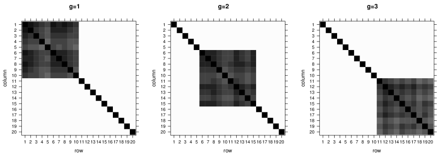
(a) Scenario 1

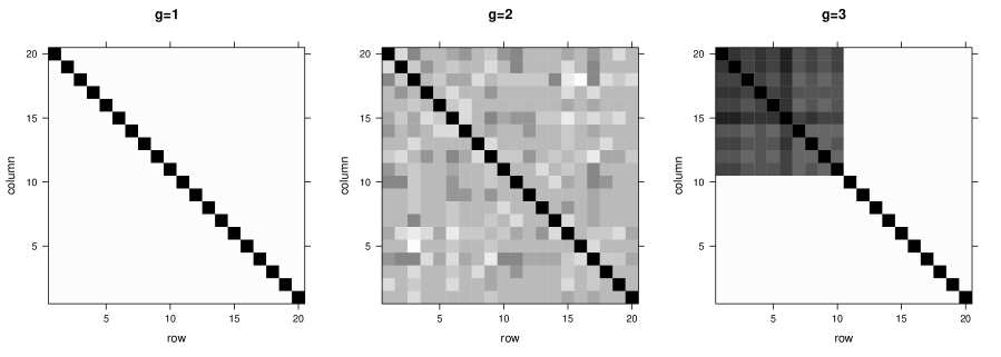
(b) Scenario 2

Figure 2: Heat maps of the true component covariance matrices in the two scenarios.

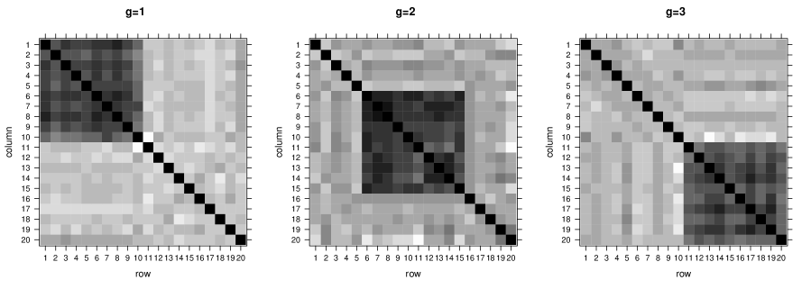
(a) $n_{g}=50$

(b) $n_{g}=100$

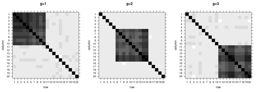
(c) $n_{g}=150$

Figure 3: Heat maps of the estimated component covariance matrices in Scenario 1 for each sample size.

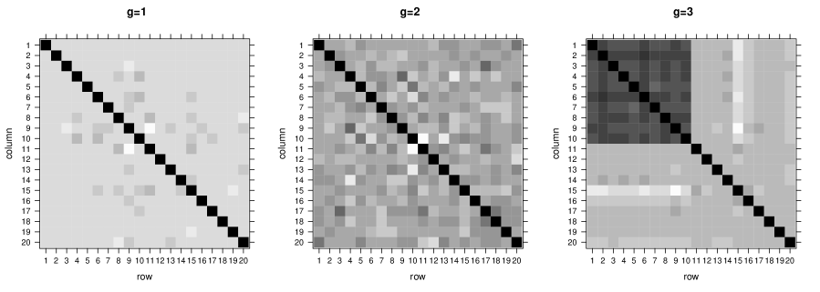
(a) $n_{g}=50$

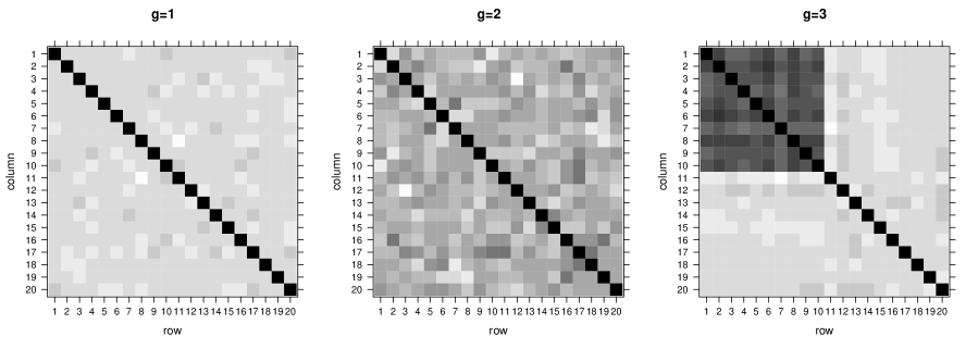
(b) $n_{g}=100$

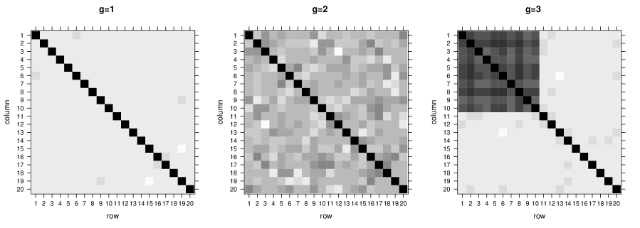
(c) $n_{g}=150$

Figure 4: Heat maps of the estimated component covariance matrices in Scenario 2 for each sample size.

4.3 Experiment 3

In this experiment, we compare our proposed approach with four approaches from recent development in model-based clustering: PGMM, FM-CFUST, MGHD, and MGHFA. PGMM is developed for high-dimensional symmetrical data via the mixture of Gaussian factor models. FM-CFUST, MGHD, and MGHFA contain parameters for capturing skewness and heavy-tail in the data, therefore, provide a flexible family of models to handle non-normal data. Two scenarios are considered: we generate a set of 100 samples from the mixture of GHD distributions (Scenario 3) as well as a set of 100 samples from the mixture of Gaussian distributions (Scenario 4). Each combination of $n_{g}$ and $p$ is considered from a three-component mixture model with the alternated-blocks sparse covariance matrices presented in Fig 2 (a). We choose to stop at $p=100$ because FM-CFUST and MGHD have convergence issues consistently when $p=50,100$.

Table 2 and 3 show the averaged BIC and ARI over the 100 samples in Scenario 3 and 4, respectively. FM-CFUST and MGHD fail to converge when the dimension of the samples reaches 50 in both scenarios. For the samples generated from the mixture of GHD distributions (Scenario 3), the GHD-GLS approach yields excellent classification on all occasions. PGMM and MGHFA are effective in dimension reduction; however, the classification results are not as good as GHD-GLS because the high-dimensional data is only explained by one or two factors ($q=1,2$). In Scenario 4, not surprisingly, PGMM performs the best among all five approaches because the samples are generated from Gaussian mixtures. The classification results for the GHD-GSL approach surpass the MGHFA on all occasions.

Table 2: A comparison of the selected GHD-GLS, PGMM, FM-CFUST, MGHD and MGHFA in Scenario 3 (replications=100).

		GHD-GLS		PGMM		FM-CFUST		MGHD		MGHFA
		BIC	ARI	BIC	ARI	BIC	ARI	BIC	ARI	BIC	ARI
$p=20$	$n_{g}=50$	5483	1	5209	0.86	5975	1	5816	NA	5208	0.91
	$n_{g}=100$	20889	1	20550	0.92	21792	1	21014	0.89	20369	0.97
	$n_{g}=150$	28502	1	25829	0.92	29399	1	29388	0.97	25366	0.94
$p=50$	$n_{g}=50$	23802	1	21885	0.80	NA	NA	NA	NA	21663	0.86
	$n_{g}=100$	44388	1	42425	0.86	NA	NA	NA	NA	40829	0.87
	$n_{g}=150$	98691	1	92311	0.87	98239	0.97	NA	NA	91190	0.95
$p=100$	$n_{g}=50$	84256	0.98	43422	0.80	NA	NA	NA	NA	41487	0.80
	$n_{g}=100$	134257	0.98	95229	0.81	NA	NA	NA	NA	92147	0.82
	$n_{g}=150$	212595	0.98	123168	0.81	NA	NA	NA	NA	120145	0.82

Table 3: A comparison of the selected GHD-GLS, PGMM, FM-CFUST, MGHD and MGHFA in Scenario 4 (replications=100).

		GHD-GLS		PGMM		FM-CFUST		MGHD		MGHFA
		BIC	ARI	BIC	ARI	BIC	ARI	BIC	ARI	BIC	ARI
$p=20$	$n_{g}=50$	5160	0.90	5080	0.95	5132	0.92	5499	0.90	5071	0.89
	$n_{g}=100$	21707	0.98	20331	0.98	21759	0.98	21755	0.97	20401	0.96
	$n_{g}=150$	26155	0.97	25595	1	29345	0.96	27614	0.97	25495	0.96
$p=50$	$n_{g}=50$	24809	0.88	21321	0.96	NA	NA	NA	NA	21421	0.86
	$n_{g}=100$	47756	0.94	41127	1	NA	NA	NA	NA	41604	0.87
	$n_{g}=150$	97409	0.93	92360	1	NA	NA	NA	NA	92346	0.92
$p=100$	$n_{g}=50$	83244	0.86	43744	0.97	NA	NA	NA	NA	44311	0.79
	$n_{g}=100$	88326	0.96	51268	1	NA	NA	NA	NA	55570	0.83
	$n_{g}=150$	208175	0.96	124958	1	NA	NA	NA	NA	137773	0.83

5 Real Data Analyses

5.1 Overview

We compare our approach with two methods based on the GHDs: MGHD and MGHFA. The Movehub quality of life data (Sect. 5.2) is selected to demonstrate the interpretability of our proposed approach. Furthermore, we use the breast cancer diagnostic data because of its popularity as a benchmark data set within the literature.

5.2 Movehub Quality of Life

The Movehub quality of life data consists of five key metrics for 216 cities (i.e., $n=216$ and $p=5$): purchase power, health care, pollution, quality of life and crime rate. An overall rating for a city is given considering all five metrics. The data is published on www.movehub.com. Our proposed GHD-GLS, MGHD, and MGHFA are fitted to these data for $G=1,\ldots,6$ and $q=1,\ldots,3$ for MGHFA. The minimum BIC occurs at $G=2$ for all three approaches. A cross-tabulation of the predicted classification from the three approaches is shown in Table 4. Table 5 presents the mean and standard deviation of the five metrics as well as the overall rating for each group.

Group 1 consists of cities with lower ratings in purchase power, health care and quality of life, while having higher ratings in pollution and crime rate. The overall rating for the cities in Group 1 is lower when compared to Group 2. Fig. 5 shows the sparse correlation structures among the five variables differ across groups which can only be found using the GHD-GLS approach. In particular, Group 1 is characterized by the relation between quality of life, crime rate, and purchase power, and Group 2 is characterized by the relation between quality of life, health care, and purchase power.

The predicted classification from our approach agrees with MGHD on all cities except for Barcelona, Curitiba and Braga. This classification result shows that GHD-GLS performs well in low dimensional data; in particular, it does not over-penalize the model parameters due to the flexibility in estimating the degree of regularization. MGHFA, however, yields a different result, classifying 18 cities into Group 1 when they belong to Group 2 using GHD-GLS. The 18 cities are: Johannesburg, Fortaleze, Noida, Rotterdam, Pretoria, Paris, London, Dublin, New York, Haifa, Curitiba, Bristol, Nicosia, Belfast, Malmo, Brighton, Seoul and Braga. Some of the cites have a very high overall rating, such as London, Paris and New York.

Table 4: A comparison of the selected GHD-GLS, MGHD and MGHFA on the quality of life data.

GHD-GLS	MGHD			MGHFA
	Group 1	Group 2		Group 1	Group 2
Group 1	85	1		86	0
Group 2	2	128		18	112

Table 5: Mean and standard deviation of the five key metrics for each component of the three approaches.

Group 1
	GHD-GLS		MGHD		MGHFA
	Mean	Std. dev.	Mean	Std. dev.	Mean	Std. dev.
Overall Rating	73.5	4.18	73.4	4.03	75.2	5.98
Purchase Power	25.2	8.67	25.1	8.42	29.1	12.15
Health Care	59.6	15.93	59.7	15.87	60.5	15.87
Pollution	56.2	23.95	55.2	24.28	54.4	24.53
Quality of Life	37.5	13.91	37.9	14.40	41.2	15.60
Crime Rate	45.7	15.34	45.4	15.54	46.4	16.08
Group 2
	GHD-GLS		MGHD		MGHFA
	Mean	Std. dev.	Mean	Std. dev.	Mean	Std. dev.
Overall Rating	83.8	4.03	83.9	3.92	83.6	3.48
Purchase Power	60.6	12.46	60.9	12.08	62.3	11.93
Health Care	70.9	11.31	70.9	11.36	71.9	10.20
Pollution	38.0	23.70	38.4	23.88	36.8	23.19
Quality of Life	74.9	10.88	74.8	11.09	77.5	8.48
Crime Rate	38.4	16.50	38.5	16.46	36.6	15.34

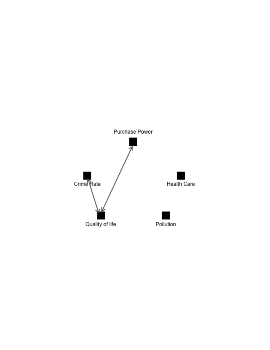
(a) Group 1

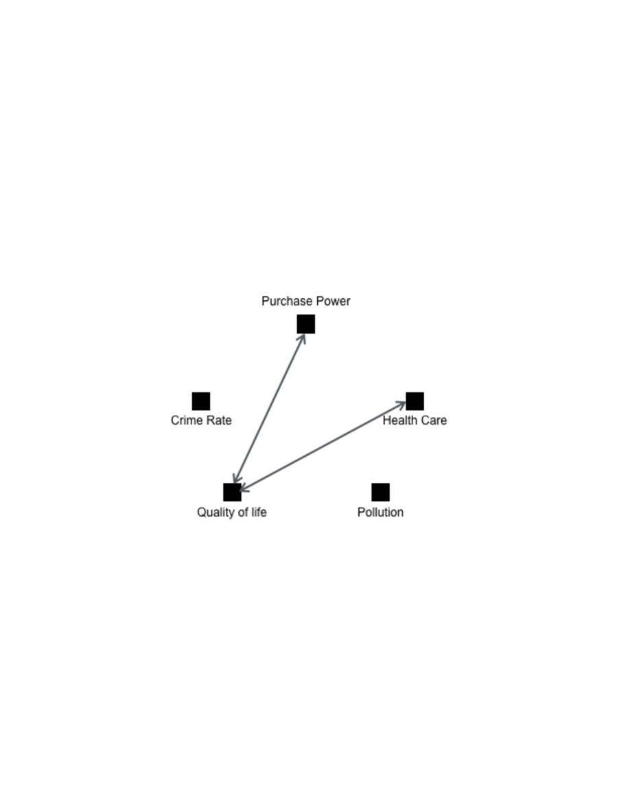
(b) Group 2

Figure 5: The correlation structures among the five variables for each group for the quality of life data using the GHD-GLS approach.

5.3 Breast Cancer Diagnostic Data Set

The breast cancer diagnostic data was first used in Street et al. (1993). Ten real-valued features on 569 cases of breast tumours are reported – 357 benign and 212 malignant. The mean, standard error, and “worst” or largest of these features were computed for each image, resulting in 30 attributes. The GHD-GLS approach is fitted to these data for $G=1,2,\dots,6$. The lowest BIC occurs at the two-component model. A summary of the best models from GHD-GLS, MGHD and MGHFA approaches is shown in Table 6. The GHD-GLS and MGHD approaches give the correct number of components (i.e., $G=2$). The GHD-GLS yields the best ARI among the three approaches (ARI=0.79). The GHD-GLS misclassifies only 32 out of 569 observations (Table 7).

Table 6: A comparison of the selected GHD-GLS and two different approaches on the tumour data.

	$G$	BIC	ARI
GHD-GLS	$2$	$30917$	$0.79$
MGHD	$2$	$36594$	$0.66$
MGHFA	$5$	$13777$	$0.58$

Table 7: Cross-tabulation of true versus predicted (A,B) classifications from the selected GHD-GLS for the tumour data.

	A	B	ARI
Malignant	352	5	0.79
Benign	27	185

6 Discussion

The GHD-GLS approach for flexible clustering of high-dimensional data was introduced. We developed the GHD-GLS based on a mixture of GHDs while including a penalty term in the likelihood constraining the component-specified concentration matrices, which enables the association structure of variables vary across the mixture components. The gamma-Lasso penalty proposed herein, enabled us to develop an analytically feasible EM algorithm. The BIC with effective number of non-zero parameters was used for model selection. The first simulation study investigated the model’s sensitivity to different values of the gamma hyperparameters as well as the effectiveness of BIC in choosing the correct model. We showed good performance on estimating the sparse component covariance matrices in Experiment 2. Comparing the GHD-GLS, PGMM, FM-CFUST, MGHD, and MGHFA yielded some interesting results. When the dimensionality was low, the FM-CFUST and MGHD approach gave similar classification results when compared to GHD-GLS. However, the GHD-GLS was able to find different sparse correlation structures among variables, leading to a simpler interpretation of the clustering results. Moreover, in Experiment 3, we showed the FM-CFUST and MGHD failed to converge consistently when the dimensionality reached 50. Although the PGMM and MGHFA were able to fit higher dimensional data, it required a pre-specified dimension of the latent variables. When fitted to the breast cancer diagnostic data, the GHD-GLS approach gave superior classification performance when compared to the chosen MGHD and MGHFA.

References

- Aitken (1926) Aitken, A. C.: A series formula for the roots of algebraic and transcendental equations. Proceedings of the Royal Society of Edinburgh 45, 14–22 (1926)
- Andrews and McNicholas (2011) Andrews, J. L., McNicholas, P. D.: Extending mixtures of multivariate t-factor analyzers. Statistics and Computing 21(3), 361–373 (2011)
- Andrews and McNicholas (2012) Andrews, J. L., McNicholas, P. D.: Model-based clustering, classification, and discriminant analysis via mixtures of multivariate -distributions: The EIGEN family. Statistics and Computing 22(5), 1021–1029 (2012)
- Banerjee et al. (2008) Banerjee, O., Ghaoui, L. E., d’Aspremont, A.: Model selection through sparse maximum likelihood estimation. Journal of Machine Learning Research 9, 485–516 (2008)
- Baum et al. (1970) Baum, L. E., Petrie, T., Soules, G., Weiss, N.: A maximization technique occurring in the statistical analysis of probabilistic functions of Markov chains. Annals of Mathematical Statistics 41, 164–171 (1970)
- Bhattacharya and McNicholas (2014) Bhattacharya, S., McNicholas, P. D.: A lasso-penalized BIC for mixture model selection. Advances in Data Analysis and Classification 8(1), 45–61 (2014)
- Böhning et al. (1994) Böhning, D., Dietz, E., Schaub, R., Schlattmann, P., Lindsay, B.: The distribution of the likelihood ratio for mixtures of densities from the one-parameter exponential family. Annals of the Institute of Statistical Mathematics 46, 373–388 (1994)
- Bouveyron and Brunet-Saumard (2014) Bouveyron, C., Brunet-Saumard, C.: Model-based clustering of high-dimensional data: A review. Computational Statistics & Data Analysis 71, 52–78 (2014)
- Bouveyron et al. (2007) Bouveyron, C., Girard, S., Schmid, C.: High-dimensional data clustering. Computational Statistics & Data Analysis 52(1), 502–519 (2007)
- Browne and McNicholas (2015) Browne, R. P., McNicholas, P. D.: A mixture of generalized hyperbolic distributions. Canadian Journal of Statistics 43(2), 176–198 (2015)
- Celeux and Govaert (1995) Celeux, G. Govaert G.: Gaussian parsimonious clustering models. Pattern Recognition 28(5), 781–793 (1995)
- Dang et al. (2015) Dang, U. J., Browne, R. P., McNicholas, P. D.: Mixtures of multivariate power exponential distributions. Biometrics 71(4), 1081–1089 (2015)
- Dempster et al. (1977) Dempster, A. P., Laird, N. M., Rubin, D. B.: Maximum likelihood from incomplete data via the EM algorithm. Journal of the Royal Statistical Society: Series B 39(1), 1–38 (1977)
- Friedman et al. (2008) Friedman, J., Hastie, T., Tibshirani, R.: Sparse inverse covariance estimation with the graphical lasso. Biostatistics 9(3), 432–441 (2008)
- Hubert and Arabie (1985) Hubert, L., Arabie, P.: Comparing partitions. Journal of Classification 2(1), 193–218 (1985)
- Karlis and Santourian (2009) Karlis, D., Santourian A.: Model-based clustering with non-elliptically contoured distributions. Statistics and Computing 19(1), 73–83 (2009)
- Krishnamurthy (2011) Krishnamurthy, A.: High-dimensional clustering with sparse gaussian mixture models. Unpublished paper pp. 191–192 (2011)
- Lee and McLachlan (2016) Lee, S., McLachlan, G. J.: Finite mixtures of canonical fundamental skew t-distributions. Statistics and Computing 26, 573–289 (2016)
- Lee and McLachlan (2015) Lee, S., McLachlan, G. J.: EMMIXcskew: an R package for the fitting of a mixture of canonical fundamental skew t-distributions. arXiv preprint arXiv:1509.02069 (2015)
- Lee and McLachlan (2014) Lee, S., McLachlan, G. J.: Finite mixtures of multivariate skew t-distributions: some recent and new results. Statistics and Computing 24, 181–202 (2014)
- Lin (2010) Lin, T.-I.: Robust mixture modeling using multivariate skew t distributions tatistics and Computing 20(3), 343–356 (2010)
- Lin et al. (2014) Lin, T.-I., McNicholas, P. D., Hsiu, J. H.: Capturing patterns via parsimonious t mixture models. Statistics and Probability Letters 88, 80–87 (2014)
- Lindsay (1995) Lindsay, B. G.: Mixture models: Theory, geometry and applications. in ‘NSF-CBMS Regional Conference Series in Probability and Statistics Vol. 5, Hayward, California: Institute of Mathematical Statistics (1995)
- McNicholas (2016) McNicholas, P. D.: Mixture Model-Based Classification. Chapman & Hall/CRC Press, Boca Raton (2016a)
- McNicholas (2016b) McNicholas, P. D.: Model-based clustering. Journal of Classification 33(3), 331–373 (2016b)
- McNicholas et al. (2011) McNicholas, P. D., Jampani, K. R., McDaid, A. F., Murphy, T. B., and Banks, L.: pgmm: Parsimonious Gaussian mixture models. R package 1 (2011)
- McNicholas et al. (2010) McNicholas, P. D., Murphy, T. B., McDaid, A. F., Frost, D.: Serial and parallel implementations of model-based clustering via parsimonious Gaussian mixture models. Computational Statistics and Data Analysis 54(3), 711–723 (2010)
- McNicholas and Murphy (2008) McNicholas, P. D., Murphy, T. B.: Parsimonious Gaussian mixture models. Statistics and Computing 18(3), 285–296 (2008)
- Murray et al. (2014b) Murray, P. M., Browne, R. B., McNicholas, P. D.: Mixtures of skew-t factor analyzers. Computational Statistics and Data Analysis 77, 326–335 (2014b)
- Murray et al. (2014a) Murray, P. M., McNicholas, P. D., Browne, R. B.: A mixture of common skew- factor analyzers. Stat 3(1), 68–82 (2014a)
- Peel and McLachlan (2000) Peel, D., McLachlan, G. J.: Robust mixture modelling using the t distribution. Statistics and Computing 10(4), 339–348 (2000)
- Schwarz (1978) Schwarz, G.: Estimating the dimension of a model. The Annals of Statistics 6(2), 461–464 (1978)
- Scott and Symons (1971) Scott, A. J., Symons, M. J.: Clustering methods based on likelihood ratio criteria. Biometrics 27, 387–397 (1971)
- Street et al. (1993) Street, N. W., Wolberg, W. H., Mangasarian, O. L.: Nuclear feature extraction for breast tumor diagnosis. IS&T/SPIE’s Symposium on Electronic Imaging: Science and Technology San Jose, California, vol. 1905, 861–870 (1993)
- Tiedeman (1955) Tiedeman, D. V.: On the study of types. in S. B. Sells, ed., ‘Symposium on Pattern Analysis’, Air University, U.S.A.F. School of Aviation Medicine, Randolph Field, Texas (1955)
- Tortora et al. (2016) Tortora, C., McNicholas, P. D., Browne, R. P.: A mixture of generalized hyperbolic factor analyzers. Advances in Data Analysis and Classification 10(4), 423–440 (2016)
- Tortora et al. (2017) Tortora, C., ElSherbiny, A., Browne, R. P., Franczak, B. C., McNicholas, P.D.: MixGHD: Model Based Clustering, Classification and Discriminant Analysis Using the Mixture of Generalized Hyperbolic Distributions, R package version 2.1 (2017)
- Vrbik and McNicholas (2012) Vrbik, I., McNicholas, P. D.: Analytic calculations for the EM algorithm for multivariate skew-t mixture models. Statistics and Probability Letters 82(6), 1169–1174 (2012)
- Vrbik and McNicholas (2014) Vrbik, I., McNicholas, P. D.: Parsimonious skew mixture models for model-based clustering and classification. Computational Statistics and Data Analysis 71, 196–210 (2014)
- Wolfe (1965) Wolfe, J. H.: A computer program for the maximum likelihood analysis of types. Technical Bulletin 65-15, U.S. Naval Personnel Research Activity (1965)