Winter Model at Finite Volume

U. G. Aglietti Dipartimento di Fisica, Università di Roma “La Sapienza”

We study Winter or $\delta$-shell model at finite volume (length), describing a small resonating cavity weakly-coupled to a large one. For generic values of the coupling, a resonance of the usual model corresponds, in the finite-volume case, to a compression of the spectral lines; for specific values of the coupling, a resonance corresponds instead to a degenerate or a quasi-degenerate doublet. A secular term of the form $g^{3}N$ occurs in the perturbative expansion of the momenta (or of the energies) of the particle at third order in $g$, where $g$ is the coupling among the cavities and $N$ is the ratio of the length of the large cavity over the length of the small one. These secular terms, which tend to spoil the convergence of the perturbative series in the large volume case, $N\gg 1$, are resummed to all orders in $g$ by means of standard multi-scale methods. The resulting improved perturbative expansions provide a rather complete analytic description of resonance dynamics at finite volume.

1 Introduction

According to the superposition principle of quantum mechanics, an arbitrary linear combination of wavefunctions of a physical system describes a possible, i.e. admissible, state of the latter. Whether such a state is physically realizable or not, it just depends on experimental facilities — ultimately on technological ability. In general, the superposition principle implies a radical departure from classical mechanics, where particles are completely localized in space at any time [1]. Stringent checks on the linear structure of quantum mechanics are provided by the flavor oscillation phenomena in neutral kaon and beauty mesons [2]; a small non linearity in the time-evolution of these systems would produce higher-order harmonics in the wavefunction (typically second and third-order ones), which have never been observed. Historically, quantum mechanics was created to describe the stationary states — as well as the transitions — of atoms and molecules and it was thought as the correct general theory of micro-systems, in contrast to classical mechanics, relegated to describe macroscopic systems only. However, as well known, there is not any spatial or temporal upper limit to the coherence phenomena implied by the superposition principle. In other words, while in quantum mechanics — as formulated nowadays — there exists, in comparison to classical physics, a new scale controlling the phenomena at small distances — namely the Planck constant or ”quantum of action” $h$ —, there is not any scale associated to the loss of coherence at long distances and/or large times. If we consider for example a crystal — let’s say a semiconductor — limitation to coherence in electron motion is usually produced by thermal effects, lattice defects and impurities present in the sample, which produce phase randomization of the wavefunction components, as well as localized states, all effects having the tendency to destroy the long-range coherence in the system. At the beginning of last century, when technology made it possible to liquefy helium, superconductivity was accidentally discovered in the study of the low-temperature dependence of electric conductivity in metals, and a first example of a macroscopic quantum system was found. Nowadays, the superfluid transition at low temperatures of the bosonic isotope of Helium (He₄) and, at much lower temperatures, the superfluid phases of the fermionic one (He₃), the Bose-Einstein condensation of alkali gases, etc. are all well-known examples of macroscopic or mesoscopic quantum systems. In more recent times, the possibility of constructing potential barriers on the scale of atomic size or so by means of sophisticated growing techniques has given rise to a new application of quantum mechanics — the so-called nanophysics.

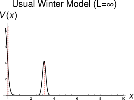
Figure 1: potential energy of standard Winter model, at infinite volume (length $L=\infty$), or equivalently, if we work in momentum space, in the continuum, for a value of the coupling of the cavity $([0,\pi])$ to the continuum $([\pi,\infty))$ $g=0.2$ (see eq. 1). For easy of visualization, the Dirac $\delta$-potential centered at the point $x=\pi$ is approximated by a sharp Gaussian distribution (standard deviation $\sigma=0.15$) with mean value at $x=\pi$. The vanishing boundary condition of the wavefunction at the origin, $\psi(x=0;t)\equiv 0$, is represented by a high and thick potential wall at $x<0$.

A typical quantum phenomenon is the decay of a resonant state — such as a naturally unstable nucleus or elementary particle, or a stable particle confined between high but slightly penetrable potential walls (tunnel effect). An unstable state is a specific narrow energy wavepacket, whose dynamics at large times is controlled by the interference of the hamiltonian eigenstates with slightly different energies. Because of additional wave reflection and interference phenomena, even deeper coherence phenomena can be investigated in quantum mechanics by studying the decay of resonant states at finite, rather than infinite, volume.

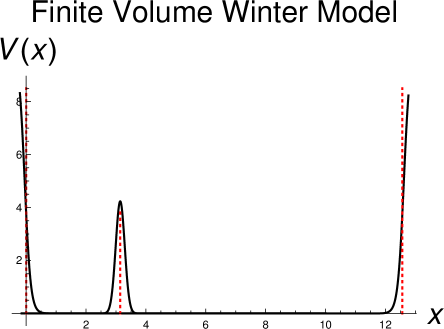
Figure 2: potential energy of finite-volume Winter model for $L=4\pi$, i.e. for the large cavity ($x>\pi$, to the right of the peak) three times bigger than the small one ($x<\pi$, on the left), for $g=0.2$. For visualization purposes, as in previous plot, the Dirac $\delta$-potential is approximated by a sharp Gaussian distribution centered at $x=\pi$, while the vanishing boundary conditions of the wavefunction at the borders of the segment $[0,L]$, $\psi(x=0;t)\equiv\psi(x=L;t)\equiv 0$, are represented by high and thick potential walls at $x<0$ and at $x>L$ respectively.

It is in this spirit that we study in this paper resonance phenomena in the generalization to finite volume of the so-called Winter (or $\delta$-shell) model. The latter is a one-dimensional quantum-mechanical model, describing the coupling of a resonating cavity to a continuum of states, with Hamiltonian given, in proper units, by the operator [3] (see fig. 1)

$$\hat{H}\,=\,-\,\frac{\partial^{2}}{\partial x^{2}}\,+\,\frac{1}{\pi g}\,\delta(x-\pi);$$ (1)

where $\delta(z)$ is the Dirac $\delta$-function centered in the origin and $g\neq 0$ is a real coupling constant. The motion of the particle is restricted to the positive half-line,

$$0\,\leq\,x\,<\,\infty,$$ (2)

and its wavefunction is assumed to vanish at the space origin at all times:

$$\psi\left(x=0;\,t\right)\,\equiv\,0;\qquad t\,\in\,{\mathbb{R}}.$$ (3)

Note that standard Winter model is a one-parameter model — namely the coupling $g$.

Because of the rather involved dynamics of finite-volume Winter model (see fig. 2), we limit ourselves in this work to the study of time-independent phenomena; we will see that the spectrum of this model contains a considerable amount of information about resonance dynamics. Rather simple analytic formulae are obtained in perturbation theory up to third order in the coupling $g$ which, when properly analyzed in combination with numerical computations, will allow us to understand some general properties of resonance dynamics at finite volume. Explicit time-dependent phenomena in finite-volume Winter model will be treated in a forthcoming publication.

It may be worth summarizing the main theoretical activity over the years concerning the standard (infinite-volume) Winter model (see fig. 1). As far as we know, this model was originally introduced in ref.[4], where the resonance spectrum in the weak-coupling repulsive regime, $0<g\ll 1$, was investigated, finding all the typical resonance phenomena [5]. The latter can be most easily described in qualitative terms as follows. In the limit $g\to 0^{+}$, the coefficient in front of the Dirac $\delta$-potential on the r.h.s. of eq.(1) diverges and the coupling of the $[0,\pi]$ cavity to the half-line $[\pi,\infty)$ exactly vanishes. In this free limit, the system approaches the union of two non-interacting subsystems: a free particle in the box $[0,\pi]$ possessing, as well known, a discrete spectrum with eigenfunctions

$$\phi_{n}(x)\,=\,\sqrt{\frac{2}{\pi}}\,\sin(nx);\qquad 0\,\leq\,x\,\leq\,\pi;\qquad n=1,2,3,\cdots;$$ (4)

and a free particle in the half-line $[\pi,\infty)$, having a continuous spectrum. If we adiabatically (i.e., in practice, very slowly) turn on the coupling from the free-theory value $g=0$ up to a very small value $g\ll 1$, the box eigenfunctions in eq.(4) go one-to-one into long-lived resonant states $(\tau\propto 1/g^{2})$, with qualitative properties similar to the former; the only qualitative difference between the box eigenfunctions and the resonant states is indeed a non vanishing width and a non-zero amplitude at $x>\pi$ of the latter. Winter model contains therefore an infinite, non-degenerate resonance spectrum at small positive coupling.

Because of tunneling effect, a particle initially in the $[0,\pi]$ cavity will leave it, ending up into the infinite region $[\pi,\infty)$. That implies that Winter model possesses in the repulsive case $g>0$, a continuous spectrum only; by explicit computation, one finds that the model contains only a continuous spectrum also in the strongly-attractive case $g<-1$. In the weakly-repulsive case, $-1<g<0$, the model possesses also a discrete spectrum, containing a single bound state, with the particle exponentially localized close to the negative barrier at $x=\pi$ [3].

R. Winter in his well-known paper [6] (see also [7] and [8]) studied the time evolution of wavefunctions $\phi(x;t)$ equal, at the initial time $t=0$, to the box eigenfunctions in eq.(4) — particle initially inside the cavity. He used both perturbative and numerical methods. An asymptotic power decay for $t\to+\infty$ was explicitly demonstrated for the first time. In ref.[3] all the calculations originally made in ref.[6] were checked, finding complete agreement as far as the exponential decay of the first resonance is concerned, as well as the asymptotic power decay of all the resonances. A disagreement was found instead in the exponential decay of the excited resonances ($n>1$) because of the occurrence of a peculiar state-mixing phenomenon. Each initial box eigenfunction (eq.(4)), labeled by the quantum number $n$, does not couple only to the corresponding resonance, of the same order $n$, but actually to all the resonances. The diagonal couplings are $1+\mathcal{O}(g)$, i.e. are large, while the off-diagonal couplings are $\mathcal{O}(g)$, i.e. small ($|g|\ll 1$), but may give rise to leading effects in large temporal regions. If we consider for example the evolution of an unstable state equal at $t=0$ to the box eigenfunction in eq.(4) with $n=2$, it is found that in a large (sub-asymptotic) temporal window, the dominant contribution to this state comes from the first resonance $(n=1)$, rather than from the second one $(n=2)$. That is because the contribution from the fundamental resonance,

$$\approx\,g\,\exp\left[-\,\Gamma_{1}(g)\,t\right],$$ (5)

even though involving a small $\mathcal{O}(g)$ coefficient, has a slower exponential time decay than the contribution coming from the first excited resonance,

$$\approx\,\exp\left[-\,\Gamma_{2}(g)\,t\right],$$ (6)

which has a large $\mathcal{O}(1)$ coefficient, but decays much faster. The decay rates $\Gamma_{n}(g)$ grow as $n^{3}$ (see later), so that

$$\Gamma_{2}(g)\,\simeq\,8\,\Gamma_{1}(g).$$ (7)

The smaller decay width $\Gamma_{1}(g)$ ”wins” the smaller expansion coefficient $\mathcal{O}(g)$. At first order in $g$, the mixing of states is controlled by an infinite real antisymmetric matrix, which was explicitly calculated in ref.[3].

In ref.[9] the idea that the resonance wavefunctions can be obtained from the simple box wavefunctions (eq.(4)) by means of finite renormalization of the parameters entering the latter, was verified by means of higher-order perturbative computations. The parameters in question are the momentum of the particle $k_{n}(g)=n+\mathcal{O}(g)$, which receives a real correction at first order in $g$ and both a real and an imaginary correction at second order, its energy $E_{n}=k_{n}^{2}$, plus an overall normalization constant $Z_{n}(g)=1+\mathcal{O}(g)$. Actually, that is nothing but the formalization of the physical idea that resonance states of the Winter model have to be close to the box eigenfunctions (i.e. are ”perturbations” of the latter) for sufficiently small couplings. Since any special orthogonal (rotation) matrix is, to first order in the angles, a real antisymmetric matrix, one may guess that the state-mixing matrix of Winter model will to be equal, after the inclusion of the higher order terms, to an infinite orthogonal matrix. By explicitly computing such a matrix to second order in $g$, it was found that, in addition to the expected iteration of the first-order matrix, there do also exist additional contributions whose interpretation in the above sense is problematic and which do not seem consistent with such an idea.

In order to understand the limitations of perturbation theory in the analysis of Winter model, the latter was studied in ref.[10] with geometrical, rather than analytical, methods. By complexifying the coupling $g$, namely

$$g\,\in\,{\mathbb{R}}\quad\mapsto\quad g\,\in\,{\mathbb{C}},$$ (9)

it was found that each resonance, anti-resonance, bound and anti-bound state of the model is related to a specific sheet of the Riemann surface of a basic transcendental infinite-valued function. In particular, by knowing the singularity structure of such surface, the convergence radii $R_{n}$’s of the expansions of the resonance momenta $k_{n}$ in powers of $g$, $k_{n}=k_{n}(g)$, were determined; they turned out to be all strictly positive, for each $n=1,2,3,\cdots$, but going to zero as $1/n$ for $n\to\infty$. For low $n$ (the cases of practical interest), the $R_{n}$’s were found to be actually one order of magnitude smaller than expected. The problem of constructing initial wavefunctions exciting exactly one resonance at a time, rather than a superposition, was also considered in ref.[10]; formally one has to invert the state-mixing matrix. Only an approximate solution of this problem was found, as well known from numerical studies (”you never fill a resonant state” [11, 12]).

As already discussed, in the weakly-attractive case, $-1\ll g<0$, Winter model contains a bound state $(bs)$ having an energy

$$E_{bs}\,\approx\,\frac{1}{g}\,\to\,-\,\infty\qquad\mathrm{for}\,\,\,g\,\to\,0^{-}.$$ (10)

The spectrum of Winter model is therefore unbounded from below in any (complete) neighborhood of the free-theory point $g=0$, and general instabilities phenomena may occur. Similar instabilities are believed to occur also in Quantum-Electro-Dynamics (QED) for any negative value of the fine structure constant, $\alpha<0$. Since an exact solution of interacting quantum field theories such as QED is beyond human abilities [13], a motivation for the study of ref.[10] was also to understand, by means of the above analogy, some properties of the vacuum structure in quantum field theory.

In ref.[14] a general expansion in powers of $1/n$ for highly-excited resonance states was introduced, where $n\gg 1$ is the excitation number ($n=1$ for the fundamental resonance). This expansion allows an approximate resummation of the perturbative series to all orders in $g$ for the decay rate of the resonances, as well as for other observables. In the case of the Winter model, the $1/n$ expansion gives for the decay rate, in Leading Order ($LO$),

$$\Gamma_{n}^{(LO)}(g)\,=\,\frac{n}{\pi}\log\left[1+(2\pi ng)^{2}\right].$$ (11)

The above formula resums all the terms of the form

$$g^{2}n^{3},\,\,g^{3}n^{4},\,\,g^{4}n^{5},\,\,\cdots,$$ (12)

i.e. with the power of $n$ minus the power of $g$ equal to one: $g^{h}n^{h+1}$, $h=1,2,3,\cdots$. By expanding the logarithm on the r.h.s. of eq.(11) in powers of $g$, one recovers the well-known lowest-order ($lo$) perturbative formula [3, 6]

$$\Gamma_{n}^{(lo)}(g)\,=\,4\pi\,n^{3}g^{2};\qquad n\,g\,\ll\,1;$$ (13)

while, for highly-excited resonances, the asymptotic $(as)$ formula is obtained [10]

$$\Gamma_{n}^{(as)}(g)\,\simeq\,\frac{2}{\pi}\,n\log\left(ng\right);\qquad n\,\gg\,\frac{1}{g}\,\gg\,1.$$ (14)

Note that, as an effect of the resummation, the leading-order $n^{3}$ growth of the width $\Gamma_{n}(g)$ with the resonance-order $n$ is converted into a much softer $n\log n$ behavior.

In refs.[11] and [15] Winter model was used as a check of general formalisms for unstable states. Even though this model is, because of the its schematizations and its low-dimensionality, mostly a mathematical-physics model, it has been used in ref.[16] for a semi-quantitative description of $\alpha$ decay in heavy nuclei. A review of generalizations of Winter model and applications of the latter to quantum chemistry can be found in the Introduction of ref.[17].

In order to make the paper reasonably self-contained and therefore accessible also to non-experts of the field, we have written a few review sections before the ones containing original results (the experienced reader may begin to read the article from sec. 5). The paper is organized as follows.

In sec. 2 we summarize the standard theory of resonances both in classical mechanics and in quantum mechanics. According to the latter, the well-known exponential decay law of unstable particles only holds approximately in an intermediate time region; the pre-exponential and the post-exponential regions are briefly described.

In sec. 3 we describe in qualitative terms the new features of resonance dynamics which occur when we go from infinite volume to finite (large) volume; in momentum space, that means to go from a continuous spectrum to a quasi-continuous spectrum of the decay channels. A typical phenomenon which occurs at finite volume is recursion in time. Given the (in principle unlimited) coherence of quantum mechanics, with some fantasy we can imagine that one day given, let’s say, the decay of a $Z^{0}$ into a muon pair,

$$Z^{0}\,\to\,\mu^{+}\,+\,\mu^{-},$$ (15)

it will be possible, by means of some experimental apparatus, to make the decay products collide with each other to produce back a $Z^{0}$,

$$\mu^{+}\,+\,\mu^{-}\,\to\,Z^{0}.$$ (16)

This ”$Z^{0}$ regeneration phenomenon” from a given decay channel provides a high-energy, ”extreme” example of a recurrence phenomenon in resonance dynamics. Recursion is actually a general phenomenon occurring in autonomous quantum systems $(\partial\hat{H}/\partial t=0)$ possessing discrete spectrum only. It is the quantum analog of the classical recurrence described by the Poincare’ theorem. A specific phenomenon of resonances at finite volume is the so-called limited quantum decay — namely the fact that, unlike at infinite volume, not all the particles in the sample eventually decay.

In sec. 4 we summarize the main features of standard Winter model (infinite volume) which, as discussed above, describes a particle confined in the segment $[0,\pi]$, between an impermeable wall (at $x=0$) and a slightly permeable one (at $x=\pi$). This simple model allows for an elementary analytic description of many typical resonant phenomena. Because of the reflecting boundary condition at the space origin (eq.(3)), the momenta $k$ of the particle are only defined up to a sign, so that we can assume for example $k>0$; that implies that the energy spectrum of standard Winter model is not degenerate.

In sec. 5 we discuss the generalization of Winter model to finite volume (see fig. 2). The latter describes a small resonating cavity weakly coupled to a large one; the usual model is recovered in the limit in which the length of the large cavity is sent to infinity. In this model, recursion in time is the fact that, if we put the particle initially inside the small cavity, $x\in[0,\pi]$, it will leave the latter after some characteristic time, but it will go back inside it with a probability arbitrarily close to one after a sufficiently long, but finite, evolution time.

In sec. 6 we compute the spectrum of finite-volume Winter model. Actually, for technical reasons, we consider the momentum spectrum rather than the energy spectrum ($E=k^{2}$). The momentum spectrum of the particle contains exactly-integer momenta,

$$p_{n}\,=\,n=1,2,3,\cdots,$$ (17)

for any value of the coupling $g$, which can be considered ”exceptional”. Corresponding to the exceptional momenta, there are ”exceptional eigenfunctions”, which also do not depend on $g$ and have exactly equal amplitudes inside both cavities. There are also non-integer, ordinary, momenta, which are the solutions of a real transcendental equation containing the coupling $g$ (cfr. eq.(75)). The normal eigenfunctions, corresponding to the non-integer momenta, depend explicitly on $g$; some of them have a resonating behavior, i.e. have an amplitude inside the small cavity (much) larger than inside the large one, or an anti-resonating behavior, i.e. they have a small-cavity amplitude smaller than the large-cavity one. The exceptional eigenfunctions, in some sense, ”separate” the resonating eigenfunctions from the anti-resonating ones.

Since the transcendental equation satisfied by the ordinary momenta cannot be solved in closed analytic form, we derive in sec. 7 ordinary perturbative expansions for the allowed momenta $k=k(g)$ of the particle in powers of the coupling $g$. From third order in the coupling $g$ on, secular terms of the form

$$g^{3}N,\quad g^{4}N^{2},\quad g^{5}N^{3},\quad g^{6}N^{4},\cdots$$ (18)

are found in the perturbative expansion of the momenta (some coefficients may actually vanish). The parameter $N$ is the ratio of the length of the large cavity over the small one and is assumed to be integer, as the model is simpler in this case. The terms (18) tend to spoil the convergence of the perturbative expansion in the large-volume case $N\gg 1$. The control over such terms is in any case necessary to deal with the infinite-volume limit $N\to\infty$.

In sec. 8 we derive improved perturbative expansions for the quantized momenta $k=k(g)$, which approximately resum the secular terms above to all orders in $g$. By comparing ordinary and improved perturbative expansions of the momenta $k=k(g)$, with exact (numerical) computations of the latter in a large region of $g$, we find that the resummed formulae describe the spectrum much more accurately than the fixed-order ones.

Finally, in sec. 9 we draw the conclusions of our first analysis of Winter model at finite volume. We also discuss how such system can be physically realized and which phenomenology is expected.

2 Resonance Dynamics at Infinite Volume

In this section we review some general properties of resonance decay at infinite volume both in classical and quantum mechanics; more details can be found in the review [18].

2.1 Classical Mechanics

Within classical mechanics, it is not possible to describe the internal dynamics of any unstable state such as, for example, an unstable nucleus; one can only derive the well-known exponential decay law with time as follows. Given a sample of $N\gg 1$ identical nuclei, it is natural to assume that the number $dN$ of decaying ones in the elementary time interval $dt$ is proportional to $dt$ itself; if we further assume, as it is natural to do, that the nuclei do not significantly interact with each other, it follows that $dN$ is also proportional to the number $N=N(t)$ of undecayed nuclei present in the sample at the current time $t$ so that, at the end:

$$dN\,=\,-\,\Gamma\,N(t)\,dt,$$ (19)

where $\Gamma>0$ is a proportionality constant dependent on the nuclei species and, in general, also on time. However, if time $t$ is homogeneous — i.e. physics is invariant under arbitrary time translations — then $\Gamma$ cannot depend on time and is therefore a constant characterizing the nuclei under study. By integrating eq.(19) with respect to time, one immediately obtains the well-known exponential decay law:

$$N(t)\,=\,N(0)\,e^{-t/\tau};$$ (20)

where

$$\tau\,\equiv\,\frac{1}{\Gamma}$$ (21)

is the mean lifetime of the nuclei under study. The decay width $\Gamma$ enters the above equation simply as a proportionality constant, so it cannot be calculated/predicted in classical mechanics.

2.2 Quantum Mechanics

In quantum mechanics, we can say that, in general, resonances occur when a discrete state is immersed and weakly-coupled to a continuum [5, 11, 12, 18, 19, 20]. When expressed as superposition of energy eigenstates of the real (interacting) system, a resonance is represented by a narrow wave packet and is therefore a quasi-stationary state — a kind of unstable state. As discussed in the Introduction, quantum coherence plays a fundamental role in resonance dynamics; indeed, to completely destroy a resonant state, it would be sufficient to change the phase of a single (not too small) coefficient entering the spectral decomposition of its wave function.

A fundamental quantity in the study of unstable systems is the so-called No-Decay (ND) probability, defined as

$$P_{ND}(t)\,\equiv\,\left|A_{ND}(t)\right|^{2},$$ (22)

where $A_{ND}(t)$ is the No-Decay amplitude,

$$A_{ND}(t)\equiv\left\langle\psi(0)|\psi(t)\right\rangle\,\equiv\,\left\langle\psi(0)\Big{|}\hat{U}(t;0)\Big{|}\psi(0)\right\rangle,$$ (23)

with $U\left(t_{2};t_{1}\right)$ the Schrodinger time-evolution operator,

$$\hat{U}\left(t_{2};t_{1}\right)\,\equiv\,e^{-i\hat{H}\left(t_{2}-t_{1}\right)};\qquad t_{1},\,t_{2}\,\in\,{\mathbb{R}};$$ (24)

and $\hat{H}$ the Hamiltonian operator of the system assumed, for simplicity’s sake, to be time-independent ($\partial\hat{H}/\partial t\equiv 0$). The physical interpretation of eq.(23) is straightforward: given the unstable state $\left|\psi(0)\right>$, prepared at the initial time $t=0$, in order to determine the no-decay amplitude, we just project $\left|\psi(t)\right>$, the evolved state from $t=0$ to the generic time $t$, on the original, unevolved state $\left|\psi(0)\right>$. Exponential decay which, as we have seen above, is an exact law in classical physics, valid at all times, is not in general a straightforward and exact consequence of the Schrodinger evolution [21]. The point is that Schrodinger equation is a dispersive wave equation, which naturally describes oscillations in space and time, quite different from, let’s say, the heat equation, generating ”kinematically” exponential time decays. One can usually identify three different temporal regions in the decay of an unstable system in quantum mechanics, which are schematically discussed in the next sections.

2.2.1 Small-time region

Since the first derivative of the no-decay probability can be shown to vanish at the initial time $t=0$ — the so-called Zeno effect [18] —

$$\frac{dP_{ND}}{dt}(t=0)\,=\,0,$$ (25)

it follows that the latter has a quadratic dependence on time at small times,

$$P_{ND}(t)\,=\,1\,-\,c\,t^{2}\,+\,\mathcal{O}\left(t^{3}\right),$$ (26)

where $c$ is a positive constant. Since a linear term in $t$ is absent in the above equation, the particle is ”late at decay” and its decay is not exponential in this region. Unlike the intermediate and asymptotic time regions (see later), the small-time region is strongly dependent on the details of the preparation of the initial state. In physical terms, we may say that the system, once prepared at the initial time $t=0$, ”adjustes” its initial wavefunction for beginning to decay [6]. The occurrence of a time behavior of the form (26) has been experimentally verified.

2.2.2 Exponential region

This is the intermediate region where the well-known exponential decay with time occurs to a (very) good approximation:

$$P_{ND}(t)\,\simeq\,Z\,e^{-\Gamma t};$$ (27)

where $Z$ is a normalization constant $(0<Z\leq 1)$ [3, 9, 10]. The exponential behavior above which, as discussed above, holds exactly in classical physics, is true only approximately in quantum mechanics and in a limited time interval. The law described by eq.(27) is the one usually found in experiments, in the sense that experimental data turn out to be well fitted by an equation of this form up to the largest times investigated. E. Rutherford was the first one to check the above law in $\alpha$-decay of heavy nuclei for twenty lifetimes or so [11].

2.2.3 Asymptotic region

Finally, it does also exist an asymptotic region in which the no-decay probability is proportional to an inverse power of time:

$$P_{ND}(t)\,\simeq\,\frac{k}{t^{p}};\qquad t\gg 1;$$ (28)

with $k$ is a positive constant and $p$ is an integer index of order one. In the Winter model, for example, $p=3$ [3, 6, 9, 10]. In general, interference effects occur in the transition interval from the exponential region to the power, post-exponential one, where these two contributions to the no-decay probability are of comparable size.

It can be shown by means of a general argument based on analyticity properties of the Fourier Transform, that $P_{ND}(t)$ cannot decay exponentially for $t\to+\infty$ but has to decay, roughly speaking, slower than that [22]. In physical terms, we may say that the unstable particles in the sample under study decay, at very large times, less frequently than expected according to the classical reasoning. In practice, in the post-exponential region, a power behavior with time is always found, with different values of the index $p$ in the different models analyzed so far (dependent on the spin of the resonance, threshold effects, etc. [20]). However, let us remark that, in any case, time evolution completely empties the initial state asymptotically [18]:

$$\qquad\lim_{t\to+\infty}P_{ND}(t)\,=\,0\qquad\mathrm{(Infinite\,\,Volume).}$$ (29)

In other words, by waiting for a long enough time, all the unstable particles in the sample under observation are eventually found to decay. If the no-decay probability is written as a Fourier transform over the energy, the total decay at asymptotic times given by eq.(29) is just a consequence of the well-known Riemann-Lebesgue lemma of Fourier Transform Theory. Furthermore, apart from very small interference effects [6], the no-decay probability $P_{ND}=P_{ND}(t)$ is generally a strictly monotonically decreasing function of $t$.

The experimental observation of post-exponential effects as described by eq.(28) is traditionally very problematic — an obvious reason for that being that at the very large times needed for that, the signal-to-background ratio becomes quite small. It has been claimed that a decay law of the form (28) is observed in some organic molecules, but the theory is not elementary in this case and interpretation problems come into play [11]. It has also been speculated that a power behavior of the form (28) never sets in in systems where repeated measurements at different times are performed because of a quantum ”resetting” effect [18].

3 Resonance Dynamics at Finite Volume

In this section we describe some general phenomena which occur in resonance decay at finite — rather than infinite — volume; if we work in momentum space rather than in physical (configuration) space, by going to finite volume, the continuum states of the decay products of the unstable state are replaced by a set of corresponding discrete levels. If the volume is large, i.e. we are close to the continuum, the levels are closely-spaced. The simplest system consists of a discrete state immersed and weakly coupled to a Quasi-Continuum (Q.C.) of states, rather than to a Continuum (C.) of states, as in the usual, infinite-volume, case [23].

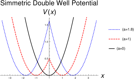
Figure 3: plots of the symmetric double well potential $V(x)=\omega^{2}\big{(}|x|-a\big{)}^{2}/2$ for $\omega=1$ and different values of the parameter $a$: $a=0$, where the potential reduces to a quadratic one (black continuous line); $a=1$ (red dashed line) and $a=1.8$ (blue dotted line).

The general problem of resonance dynamics at finite volume is also of interest in lattice quantum field theory — namely lattice QCD — where the quantum fields are regularized by introducing a finite euclidean space-time lattice [24]. The theory so constructed possesses both an ultraviolet energy/momentum cutoff $\Lambda_{UV}$, of the order of the inverse of the lattice spacing $a$,

$$\Lambda_{UV}\,\approx\,\frac{1}{a};\qquad a\,>\,0;$$ (30)

as well as an infrared cutoff $\lambda_{IR}$, given by the inverse of the lattice length $L$,

$$\lambda_{IR}\,\approx\,\frac{1}{L};\qquad L\,<\,\infty.$$ (31)

The two length scales above are related by the equation

$$L\,=\,Na,$$ (32)

where $N\gg 1$ is the number of lattice points along one of the coordinate axes (the lattice size). The unavoidable finite-size effects, $V<\infty$ or, equivalently, in energy-momentum space, $\lambda_{IR}>0$, are currently used to determine scattering quantities [25]. The main application so far developed is the calculation of $g_{\rho\pi\pi}$, the $\rho\pi\pi$ coupling entering the dominant, strong-interaction decay of the rho meson into two pions,

$$\rho\,\to\,\pi\,+\,\pi.$$ (33)

In order to understand in a simple way the relevant physics at finite volume, let us consider the scattering of a non-relativistic particle on a short-range repulsive potential $U=U(r)$. In the usual case of an infinite volume available to the particle (typically the whole space ${\mathbb{R}}^{3}$), the initial state of the particle is described, in the far past $t\approx-T$ $(T\gg 1)$, by a wavepacket far away from the potential range, with some average momentum $\bar{\bf{p}}$. When the wavepacket hits the potential $U(r)$, i.e. reaches the potential region (where the potential is significantly different from zero), let’s say at $t\approx 0$, an outgoing wave having the form of a spherical shell of thickness of the order of the packet size is generated by the interaction. By progressively increasing the time $t$ from the interaction time $t\approx 0$ up to the far future, $t\approx T$, one ends up with the the original wavepacket evolved from $-T$ to $+T$ (which has simply traveled with the average velocity $\mathbf{v}=\mathbf{p}/m$), superimposed to a spherical shell emerging out of the space origin $r=0$ from $t\approx 0$ with the radial velocity $v_{r}=\left|\bf{v}\right|$. When we go to finite volume, the energy spectrum of the system changes from a continuous to a discrete one. Furthermore, since the particle is now always at a finite distance from the potential $U(r)$, the energy levels are modified with respect to the free case $U(r)\equiv 0$; according to physical intuition, we expect such a level shift to increase by lowering the volume. While in the continuum-spectrum case (infinite volume), the potential causes transitions ($S$-matrix), in the Quasi-Continuum case (finite volume), $U(r)$ causes calculable shifts of the discrete energy levels. By looking at the spectrum of the system at different volumes, it is possible to reconstruct the scattering phases of the infinite-volume system.

In general, as one could expect according to physical intuition, by going from infinite volume to finite volume, resonance dynamics becomes far more complicated and new phenomena, which do not occur at infinite volume, come into play. The main ones are: 1. recurrence and 2. limited decay. Let us briefly discuss them in the following sections.

3.1 Time Recurrence

Time Recurrence in a quantum system can be roughly defined as the fact that the latter goes back to its initial state with arbitrary (high) degree of accuracy after a proper, sufficiently long but finite time evolution. Recurrence was originally discovered in classical mechanics, where the following theorem holds.

3.1.1 Poincare’ Theorem

In classical mechanics, the following recurrence theorem holds [26]:

Th.: given an autonomous Hamiltonian system,

$$\frac{\partial H}{\partial t}\,\equiv\,0,$$ (34)

with a finite number of degree of freedom, having a finite-volume phase space and given an arbitrary time $T>0$, an arbitrary (small) neighborhood of any initial state ($t=0$) intersects itself under the Hamiltonian flow at some time $t>T$.

In practice, a finite number of degrees of freedom means a finite number of particles and the hypothesis of finite volume of the phase space is verified for example if the particles of the system are confined into a finite region (let’s say a box) and the inter-particle potentials are bounded from below (they describe, for example, repulsive forces). In physical terms, the system goes back arbitrary close to basically all its previously reached states, after a sufficiently long evolution time. Basic questions related to this phenomenon concern the dependence of the distribution of the recursion times $\left\{t_{i}\right\}$ on the number of degrees of freedom in the system and on the kind of interactions. In general, the recursion times grow exponentially with the number of degrees of freedom of the system [26]. It would also be interesting to know the size of the time slices $\left\{\delta t_{i}\right\}$ where recurrence holds.

3.1.2 Quantum Recurrence Theorem

Even though phase space does not exist in quantum mechanics, an analog theorem to the Poincare’ one holds true [27]:

Th.: if a quantum system, described by an Hamiltonian operator $\hat{H}$, is autonomous,

$$\frac{\partial\hat{H}}{\partial t}\,=\,0,$$ (35)

and possess a discrete spectrum only, then its comes back to anyone of its previously-reached states, in quadratic norm, as close as we desire, after a sufficiently long evolution time $t$ larger than any given threshold $T>0$.

The following remarks are in order.

1. The hypothesis of time independence of the Hamiltonian function/operator is the same in the classical and in the quantum cases.

2. The assumption, in the quantum case, of discrete spectrum only is the natural translation of the condition of finite volume of phase space of the classical system.

In order to understand the physical meaning of this theorem, let us sketch its proof, which is based on the theory of almost-periodic functions [28]. By expanding a general wavefunction $\phi$ of the system under consideration in energy eigenstates $\left\{\psi_{n}\right\}$, one obtains:

$$\phi(x,t)\,=\,\sum_{n=1}^{\infty}a_{n}\,\psi_{n}(x)\,e^{-i\omega_{n}t};$$ (36)

where the coefficients $a_{n}\in{\mathbb{C}}$ satisfy the completeness relation

$$\sum_{n=1}^{\infty}\left|a_{n}\right|^{2}\,=\,1.$$ (37)

We have assumed that the initial wavefunction and the eigenfunctions of the system are normalized to one:

$$\|\phi\|\,=\,1;\qquad\left\|\psi_{n}\right\|\,=\,1;\qquad n=1,2,3,\cdots.$$ (38)

Without any generality loss, we can assume the frequencies (energies) of the system to be ordered

$$\qquad\qquad\omega_{n}\,\leq\,\omega_{n+1};\qquad n=1,2,3,\cdots.$$ (39)

As far as the time variable $t$ is concerned, the expansion on the r.h.s. of eq.(36) is a Generalized Fourier Series, the latter being defined by a formal trigonometric series of the form

$$f(t)\,\sim\,\sum_{n=1}^{\infty}c_{n}\,e^{-i\omega_{n}t},$$ (40)

with the $c_{n}$’s arbitrary (complex) coefficients. Since the frequencies $\left\{\omega_{n}\right\}$ have generically irrational ratios,

$$\frac{\omega_{m}}{\omega_{n}}\,\notin\,{\mathbb{Q}};\qquad m\,\neq\,n;$$ (41)

the function $f=f(t)$ is not a periodic function of the time $t$. Since, according to eq.(37), the series on the r.h.s. of eq.(36) is convergent (in quadratic norm), we can approximate the wavefunction $\phi(x,t)$, as accurately as we wish, by neglecting sufficiently small coefficients; the function series on the r.h.s. of eq.(36) then becomes a finite (possibly big) sum:

$$\phi(x,t)\,\simeq\,\sum_{k=1}^{N}a_{n_{k}}\,\psi_{n_{k}}(x)\,e^{-i\omega_{n_{k}}t};$$ (44)

As well known in the theory of almost-periodic functions, the frequencies occurring in such a finite sum,

$$\omega_{n_{1}},\,\omega_{n_{2}},\,\cdots,\omega_{n_{N}},$$ (45)

can be simultaneously approximated, with arbitrary accuracy, by means of a sequence of rational numbers with a small, common denominator $M$,

$$\omega_{n_{k}}\,\simeq\,\Omega_{k}\,\equiv\,\frac{m_{k}}{M}\,\in\,{\mathbb{Q}};\qquad m_{k},\,M\,\in\,{\mathbb{N}};\qquad k=1,2,\cdots,N.$$ (46)

In this way we obtain an (exactly) periodic function of time with period $T=2\pi/M$, which provides the required approximation:

$$\phi(x,t)\,\,\approx\,\,\varphi(x,t)\,\equiv\,\sum_{k=1}^{N}a_{n_{k}}\,\psi_{n_{k}}(x)\,\exp\left(-i\,\frac{m_{k}}{M}\,t\right).$$ (47)

As in the classical case, also in the quantum case it is interesting, once fixed a degree of accuracy (error), to determine the recurrence times $\left\{t_{i}\right\}$ of the states of the system, together with the size of the time slices $\left\{\delta t_{i}\right\}$ in which the wavefunction is close to the initial one.

3.1.3 Examples

In ref.[29] resonance dynamics in the quasi-continuum limit was studied in abstract form by considering a system of linear first-order ordinary differential equations (ode’s) in time, describing the evolution of the amplitude $a=a(t)$ of a discrete state coupled to quasi-continuum amplitudes $b_{i}=b_{i}(t)$, $i=1,2,\cdots,N$ $(N\gg 1)$. By assuming a simple form of the coupling terms and, as initial condition, only the discrete state to be populated at $t=0$,

$$a(t=0)\,=\,1;\qquad b_{i}(t=0)\,=\,0;\qquad i=1,2,\cdots,N$$ (48)

the model was exactly solved in terms of Laguerre polynomials and recurrence phenomena were explicitly found. In this particular case, the recurrence times can easily be determined.

3.2 Limited Decay

The second new phenomenon which occurs in resonance dynamics when we go to finite volume, is the fact that a finite fraction of unstable particles in the initial sample may not decay at any time. As discussed above, this ”failure to decay” cannot occur in the continuum case (infinite volume). Let us remark that this phenomenon is not as general as the time recurrence which we have considered in the previous section; in particular, there is not any general theorem concerning limited decay, so one just considers specific examples. Within the (of course necessarily limited) knowledge of the author, this phenomenon has been extensively discussed in ref.[30] and in ref.[31].

The time evolution of a particle in the symmetric double-well potential (see fig. 3)

$$V(x)\,=\,\frac{\omega^{2}}{2}\,\big{(}|x|-a\big{)}^{2};\qquad\omega>0;\quad a\geq 0;$$ (49)

whose spectrum had been calculated in ref.[32], was re-considered in ref.[30]. By numerically solving the Schrodinger evolution of this system with the particle initially (at $t=0$) put in the left cavity, it was found that it does exist a sequence of times at which the particle sits in the right cavity, i.e. the transition from the left cavity to the right one is complete. The symmetric potential in eq.(49) was then generalized to various asymmetric potentials with the right cavity generally larger and deeper than the left one. For some asymmetric potentials, it was found that it does not exist any time at which the transition to the right cavity is complete.

In ref.[31] resonance dynamics at Finite Volume or, equivalently, in the Quasi-Continuum limit, was studied in abstract form by means of a Hamiltonian operator $\hat{H}$ given by a big Hermitian matrix of the form

$$H\,=\,\big{(}H_{i,j}\big{)}_{i,j=0,1,2,\cdots,N}\,\equiv\,\left(\begin{array}[]{ccccc}\epsilon&g_{1}&g_{2}&\cdots&g_{n}\\ \bar{g}_{1}&\omega_{1}&0&\cdots&0\\ \bar{g}_{2}&0&\omega_{2}&\cdots&0\\ \cdots&\cdots&\cdots&\cdots&\cdots\\ \bar{g}_{N}&0&0&\cdots&\omega_{N}\end{array}\right);$$ (50)

where the over-lying bar denotes complex conjugation. The energies on the main diagonal are all real,

$$\epsilon,\,\,\omega_{1},\,\,\omega_{2},\,\,\cdots,\,\,\omega_{N}\,\in\,{\mathbb{R}}.$$ (51)

The matrix $H$ above, of order $N+1$, describes the coupling of a discrete level with energy $H_{0,0}=\epsilon$ to the Q.C. states with energies $H_{i,i}=\omega_{i}$ by means of the (in general complex) couplings given by the off-diagonal elements $H_{0,i}=g_{i}$ $(i=1,2,\cdots,N)$. Without any generality loss, the energies of the Q.C. states can be assumed to be ordered,

$$\omega_{1}\,\leq\,\omega_{2}\,\leq\,\cdots\,\leq\,\omega_{N}.$$ (52)

Furthermore, the discrete state energy $\epsilon$ is assumed to lie between the Q.C. ones,

$$\epsilon\,\in\,\left[\omega_{1},\,\omega_{N}\right],$$ (53)

or to be close to them. By taking a proper distribution of the couplings $g_{i}$ (sufficiently large and not too smooth at thresholds) and making proper choices for the diagonal elements $\epsilon$ and $\omega_{i}$, a limited quantum decay was observed at all times, together with the general time recursion phenomenon. Let us make a few remarks about this model.

1. There is not any direct coupling of the Q.C. states among themselves. That implies that, by switching off all the couplings, $g_{i}\to 0$, $i=1,2,\cdots,N$, each Q.C. state $\omega_{i}$, as well as the discrete state $\epsilon$, ”evolves diagonally”, i.e. it becomes an eigenstate of $H$.

2. The matrix $H$ given in eq.(50) is actually the generalization to the Quasi-Continuum case of the Continuum Hamiltonian model originally introduced in ref.[23].

In the study of resonance dynamics in the Q.C. limit, i.e. at finite but large volume, it would also be interesting to determine whether there exist some temporal regions where the decay is, within a reasonable approximation, exponential in time, as well as to investigate whether the Zeno effect still occurs at small times. For very large volumes, where extremely large recursion times are expected, if an exponential region is found, one could also try to identify a post-exponential, power-decay region, if any.

4 Standard Winter Model

By standard Winter model we mean the usual Winter model at infinite volume or, if we work in momentum space, in the Continuum. The Hamiltonian operator of the model and the boundary conditions on the wavefunctions have been given in eq.(1) and in eq.(3) of the Introduction respectively, so we do not repeat them here. As far as dynamics is concerned, we may say that the particle undergoes a perfect, i.e. complete, reflection at the space origin, $x=0$, and an almost-perfect reflection at the potential barrier, $x=\pi$, if the coupling is small, $0<g\ll 1$ (for simplicity’s sake, we restrict ourselves to a repulsive interaction). In each collision of the particle with the barrier at $x=\pi$, in addition to a large reflected wave, a small transmitted wave is also generated because of tunneling effect.

4.1 Strong-Coupling Limit

In the strong-coupling limit of the model,

$$g\,\to\,+\,\infty,$$ (54)

the potential barrier at $x=\pi$ disappears, so that

$$\hat{H}_{g=\infty}\,=\,-\,\frac{\partial^{2}}{\partial x^{2}},$$ (55)

and the system reduces to a free particle on the half-line

$$0\,\leq\,x\,<\,\infty.$$ (56)

The latter, as well known, possesses a continuous, non-degenerate energy spectrum with eigenfunctions

$$\Phi_{k}(x;t)\,=\,\sqrt{\frac{2}{\pi}}\sin\left(kx\right)\,e^{-ik^{2}t};\qquad k\,\in\,{\mathbb{R}}^{+}.$$ (57)

We have assumed the (conventional) continuum normalization:

$$\left\langle\Phi_{p}\big{|}\Phi_{k}\right\rangle\,=\,\delta(p-k);\qquad p,\,k\,\in\,{\mathbb{R}}^{+}.$$ (58)

4.2 Weak-Coupling Limit

In the free limit,

$$g\,\to\,0^{+},$$ (59)

it turns out that the potential barrier of Winter model becomes impenetrable. Since the Hamiltonian in eq.(1) has a pole for $g\to 0$, this limit has to be studied indirectly, by calculating its eigenfunctions as functions of $g$ and then taking the free limit on them [3, 6, 9, 10]. In complete agreement with physical intuition, as anticipated in the Introduction, for $g\to 0^{+}$ the system reduces to the union of two non-interacting subsystems:

1. a free particle in the box $[0,\pi]$, having a non-degenerate discrete spectrum with (normalized to one) eigenfunctions

   $$\phi_{n}(x;t)\,=\,\sqrt{\frac{2}{\pi}}\sin\left(nx\right)\,e^{-in^{2}t};\qquad 0\,\leq\,x\,\leq\,\pi;\qquad n=1,2,3,\cdots.$$ (60)

2. a free particle in the half line $[\pi,\infty)$, possessing a non-degenerate continuous spectrum with eigenfunctions

   $$\varphi_{k}(x;t)\,=\,\sqrt{\frac{2}{\pi}}\sin\big{[}k(x-\pi)\big{]}\,e^{-ik^{2}t};\qquad\pi\,\leq\,x\,<\,\infty;\qquad k>0.$$ (61)

   The latter are normalized as in the previous section as:

   $$\left\langle\varphi_{p}\big{|}\varphi_{k}\right\rangle\,=\,\delta(p-k);\qquad p,\,k\,>\,0.$$ (62)

4.3 Qualitative Discussion on Resonance Dynamics

As general unstable state, let us consider an initial wavefunction of the particle $(t=0)$ identically vanishing outside the $[0,\pi]$ resonating cavity:

$$\Psi(x;t=0)\,\equiv\,0\qquad\mathrm{for}\quad x\,>\,\pi.$$ (63)

One can take for example an eigenfunction of the box $[0,\pi]$ (which is nothing but the $[0,\pi]$ resonating cavity with an impenetrable barrier at $x=\pi$ also), continued to zero outside the box:

$$\Psi^{(h)}(x;t=0)\,\equiv\,\left\{\begin{array}[]{cc}\sqrt{2/\pi}\sin(hx);&0\,\leq\,x\,\leq\,\pi;\\ 0;&\,\pi\,<\,x\,<\,\infty;\end{array}\right.\qquad h=1,2,3,\cdots.$$ (64)

Since the above wavefunctions form a basis for any function $f(x)$ defined for $x\in[0,\infty)$ with support in $[0,\pi]$ only, any initial wavefunction $\Psi(x;t=0)$ possesses an expansion in terms of the set $\left\{\Psi^{(h)}(x;t=0);\,h=1,2,3,\cdots\right\}$. Therefore there is not any generality loss in considering the box eigenfunctions (eq.(64)) individually, i.e. one at a time.

The time evolution of such a wavefunction can be qualitatively described as follows. Since the potential barrier is slightly penetrable at small coupling, $0<g\ll 1$, a small component of the initial wavefunction filters through $x=\pi$ because of tunneling effect, so that an outgoing wave is generated at $x>\pi$, representing the ”decay products” of the unstable state under consideration. Because time evolution is unitary, the outgoing wave is generated ”at the expense” of the inside amplitude, i.e. the inside amplitude is diminished. Since the outgoing wave does not hit any barrier in its propagation to the right, far from the cavity, towards $x=+\infty$, the inside amplitude is never regenerated by the outgoing wave, so that the no-decay probability,

$$P_{ND}^{(h)}(t)\,\equiv\,\left|\int\limits_{0}^{\pi}\bar{\Psi}^{(h)}(x;0)\,e^{-i\hat{H}t}\,\Psi^{(h)}(x;0)\,dx\right|^{2};\qquad h=1,2,3,\cdots;$$ (65)

is basically a monotonically-decreasing function of time down to zero, in agreement with the general theory.

5 Winter Model at Finite Volume

We generalize the standard Winter model considered in the previous section, by restricting the particle coordinate $x$ to a segment,

$$0\,\leq\,x\,\leq\,L\,<\,\infty,$$ (66)

and assuming a vanishing (or reflecting) boundary condition also at the final endpoint of the segment (see fig. 2):

$$\psi(x=L;\,t)\,\equiv\,0;\qquad t\,\in\,{\mathbb{R}}.$$ (67)

The model so constructed describes a small resonating cavity ($x\in[0,\pi]$) weakly-coupled for $|g|\ll 1$ to a large one ($x\in[\pi,L]$); the resonant states of the small cavity are coupled to close, equally-spaced momentum levels. Let us remark that, while standard Winter model is a one-parameter model, its extension at finite volume is a two-parameter model — namely $g$ and $N$. However, even after the extension to finite volume, the model remains relatively simple, so that computations can still be made to some extent — as we are going to show — analytically. Winter model at infinite volume is recovered from the finite-volume model by taking the limit $L\to+\infty$.

5.1 Qualitative Discussion on Resonance Dynamics

Similarly to the infinite-volume case, let us consider an initial wavefunction identically vanishing outside the small cavity $[0,\pi]$, i.e. exactly zero inside the large cavity, for $x\in[\pi,L]$. As in the infinite-volume case, for $0<g\ll 1$, a little outgoing wave is generated at small evolution times out of the initial amplitude. By increasing time from zero up to

$$t\,\approx\,t_{one-way}\,\equiv\,\frac{L}{v}\qquad(L\gg\pi);$$ (68)

where $v$ is the average group velocity of the wavepacket, the outgoing wave propagates up to the right border of the large cavity, at $x=L$, where it is (completely) reflected back in the allowed region $[0,L]$. Such a wave, by propagating to the left, goes back towards the small cavity and then suffers at the point $x=\pi$ a large reflection and a small transmission, at the time

$$t\,\approx\,t_{two-way}\,\equiv 2\,t_{one-way}\,\equiv\,\frac{2L}{v}.$$ (69)

As in any collision of the particle with the barrier at $x=\pi$, there is a small transmitted wave because of the small permeability of the latter. A small wave component therefore goes back inside the small cavity. Such a ”regeneration phenomena” — which we have described pictorially in the Introduction with the $Z^{0}$ example — is characteristic of resonances at finite volume, as it clearly does not occur at infinite volume. The general phenomenon of time recurrence (which we have discussed in sec. 3.1) can be explained qualitatively for the present model in terms of the above dynamical mechanism: by waiting a proper, sufficiently long, evolution time, multiple reflection gives rise to an almost complete re-entering of the initial wavefunction inside the small cavity. Also the phenomenon of limited decay (which we have discussed in sec. 3.2), if it actually occurs in some parameter-space region of the finite-volume Winter model, can be explained qualitatively as follows. Let us expand the initial wavefunction of the unstable state in eigenfunctions of $\hat{H}$, the complete, interacting Hamiltonian of the system. Since the different energy components have different transmission and reflection coefficients (the latter depend upon the energy), as well as different propagation velocities, it may happen that for no times all these components are outside of the small cavity, so that the no-decay probability never vanishes.

6 Spectrum

Unlike standard Winter model, which has a continuous spectrum, finite-volume Winter model has a discrete spectrum which, as discussed in the Introduction, is naturally decomposed in an exceptional part, which we consider first, and an ordinary part.

6.1 Exceptional Eigenvalues and Eigenfunctions

It is immediate to check that the wavefunctions

$$\varphi_{n}(x)\,=\,\sqrt{\frac{2}{L}}\,\sin\left(p_{n}\,x\right);\qquad 0\,\leq\,x\,\leq\,L;$$ (70)

having the exactly-integer momenta,

$$p_{n}\,\equiv\,n\,=\,1,2,3,\cdots,$$ (71)

are eigenfunctions of the finite-volume Winter model (see fig. 4). The quantity $L$, the total length of the system, is assumed, for simplicity’s sake, to be an integer multiple of $\pi$, i.e. of the length of the small cavity,

$$L\,=\,M\pi;\qquad M\,\ \mathrm{integer}.$$ (72)

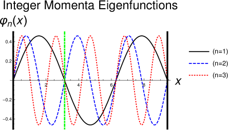
Figure 4: Plots of the first three exceptional eigenfunctions of finite-volume Winter model with the exactly integer momenta $p=1,2,3$ for $L=3\pi$, i.e. for the large cavity (to the right of the vertical thick green dot-dashed line) two times bigger than the small one (to the left of the green line). The boundaries of the system are represented by black thick continuous vertical lines.

Since all the $\varphi_{n}(x)$’s exactly vanish at $x=\pi$,

$$\varphi_{n}(x=\pi)\,\equiv\,0;\qquad n\,\in\,{\mathbb{N}};$$ (73)

the $\delta$-potential, with support at this point only, does not have any effect on the matching condition on the eigenfuctions. The consequences of this fact are the following:

1. The exceptional eigenvalues $p_{n}$ and the exceptional eigenfunctions $\varphi_{n}$ do not have any dependence on the coupling of the model $g$.

2. The eigenfunctions $\varphi_{n}(x)$ in eq.(70) are smooth functions of $x$, i.e. they have continuous space derivatives of all orders in the interval $(0,L)$,

   $$\varphi_{n}\,\in\,C^{\infty}(0,L);\qquad n\,\in\,{\mathbb{N}};$$ (74)

3. If the $\varphi_{n}$’s are restricted to the interval $[0,\pi]$, they become eigenfunctions of the free particle in the box $[0,\pi]$ (actually, all the box eigenfunctions are obtained this way). Furthermore, if the $\varphi_{n}$’s are restricted to the large cavity $[\pi,L]$, they become eigenfunctions of the free particle in the box $[\pi,L]$.

Let us end this section by noting that if the $\varphi_{n}(x)$’s are extended smoothly to the entire positive half-line, $x\in[0,\infty)$, they become eigenfunctions of the standard Winter model. However, since the spectrum of the usual model is continuous, these eigenfunctions form a negligible, zero-set measure.

6.2 Normal Eigenvalues

The quantum number $k>0$, appearing in the normal eigenfunctions $\psi(k;x)$ (see later), is a quantized, non (exactly) integer momentum, satisfying the real transcendental equation

$$\cot(\pi k)\,+\,\cot(\pi Nk)\,+\,\frac{1}{\pi gk}\,=\,0\qquad(g\neq 0);$$ (75)

where the integer

$$N\,\equiv\,M-1$$ (76)

is the length, in units of $\pi$ of the large cavity

$$[\pi,\,L]\,=\,[\pi,\,M\pi]\,=\,\left[\pi,\,(N+1)\pi\right].$$ (77)

Since all the terms appearing in eq.(75) are odd functions of $k$, it follows that, if $\bar{k}$ is a solution of eq.(75), then also $-\,\bar{k}$ is a solution of this equation. This fact is a consequence of the fact that the vanishing boundary condition at $x=0$, eq.(3), is a reflecting one, so that momentum is conserved only up to a sign. Without any generality loss, we can therefore assume

$$k\,>\,0.$$ (78)

We may say that solving eq.(75) — determining all the normal component of the momentum spectrum of finite-volume Winter model — is the main aim of this paper. We have not been able to solve this equation analytically in terms of known special functions, so we will resort to numerical and perturbative methods. An important point is to label the allowed momenta $k$ in a physically appealing way. Since for $g\to 0$, i.e. in the free limit of the model, the last term on the l.h.s. of eq.(75) diverges, it follows that the sum of the cotangent functions have to diverge also. Since $N$ is integer, the poles of $\cot(\pi k)$ are also poles of $\cot(\pi Nk)$. That implies that also the function $\cot(\pi Nk)$ diverges in the free case, so that the allowed momenta $k$ must have limiting values

$$k^{(0)}\,=\,\frac{s}{N};\qquad s\,=\,1,2,3,\cdots\qquad(g\to 0).$$ (79)

By the general principle of adiabatic continuity [33], let us therefore label all the normal momenta $k$, in the general interacting case $g\neq 0$, by the value taken for $g\to 0$:

$$k\,=\,k_{s/N}(g)$$ (80)

with

$$\lim_{g\to 0}k_{s/N}(g)\,=\,\frac{s}{N};\qquad s\,=\,1,2,3,\cdots;\quad k\,\in\,{\mathbb{R}}^{+}.$$ (81)

6.2.1 Strong-Coupling Limit

For $g\to+\,\infty$, i.e. in the strong-coupling limit, the momentum spectrum equation (75) basically simplifies into the elementary equation

$$\sin(\pi Mk)\,=\,0;$$ (82)

where we remember that

$$M\,=\,N+1$$ (83)

is the total length of the system (small cavity $+$ large cavity) in units of $\pi$. The solutions of the above equation are the momenta (see figs. 5$-$7)

$$k\,=\,\frac{s}{M},\qquad s=1,2,3,\cdots.$$ (84)

For $g\to\infty$, the potential barrier, given by the $\delta$-function, completely disappears and the system reduces to a free particle in the box $[0,L]$. The level spacing in this limit approaches the constant value

$$\Delta k_{g=\infty}\,=\,\frac{1}{N+1}.$$ (85)

Therefore, in the strong-coupling limit, the momentum spectrum of finite-volume Winter model goes into a non-degenerate, equally-spaced spectrum. When the index $s$ is an integer multiple of $M$, then the momentum in eq.(84) is integer:

$$s\,=\,n\,M\quad\Rightarrow\quad k\,=\,n;\qquad n=1,2,3,\cdots;$$ (86)

and we re-obtain the exceptional momenta.

6.2.2 Free-Theory Limit

As discussed above, for $g\to 0^{+}$, i.e. in the free limit, the allowed momenta are of the form (see figs. 5$-$7)

$$k^{(0)}\,=\,\frac{s}{N}.$$ (87)

By means of the euclidean division of $s$ by $N$,

$$s\,=\,n\,N\,+\,l,$$ (88)

the free-theory momentum can also be written in the form

$$k^{(0)}\,=\,n\,+\,\frac{l}{N}.$$ (89)

We take the remainder $l$ in the (quasi-)symmetric range

$$-\,\frac{N}{2}\,<\,l\,\leq\,\frac{N}{2}.$$ (90)

In the following, a momentum level $k$, considered as a function of the coupling $g$: $k=k(g)$, which is equal to $n+l/N$ in the limit $g\to 0$, will be called a $(n,l)$ level or more simply a $l$ level. When $s$ is an integer multiple of $N$, then the momentum in eq.(87) is integer:

$$s\,=\,n\,N\quad\Rightarrow\quad k\,=\,n;\qquad n=1,2,3,\cdots;$$ (91)

and we re-obtain the exceptional momenta. The level spacing in the free limit is given by:

$$\Delta k_{g=0}\,=\,\frac{1}{N}.$$ (92)

Note that it is larger than the strong-coupling spacing (cfr. eq.(85)). As we are going to show in the next section, the levels $k_{n}(g)$ become degenerate with the exceptional levels $p_{n}\equiv n$ in the limit $g\to 0$ and this degeneracy ”compensates” for the larger $g\to 0$ spacing, giving rise to the same average level density as for $g\to\infty$.

To summarize, in the free limit, the momentum spectrum of finite-volume Winter model goes into an equally-spaced spectrum, eq.(87), with a double degeneracy at integer momenta (eq.(91)).

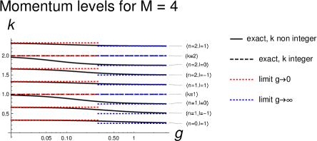
Figure 5: plots of the first nine momentum levels $k$ as functions of the coupling $g$, $k=k(g)$ (the continuous and dashed black lines), of Winter model at $M=4$, i.e. for the system with the large cavity three times bigger than the small one. The red dotted lines represent the free limit of the corresponding levels $\left(\lim_{g\to 0}k(g)\right)$, while the blue dotted lines represent the strong-coupling limit $\left(\lim_{g\to\infty}k(g)\right)$. The degeneracy for $g\to 0$ of the flat level $k\equiv 1$ (the lower black dashed line) with the resonating level $k_{1}(g)$ right below it — in an otherwise equally-spaced spectrum — is clearly visible; a similar degeneracy occurs between the level $k\equiv 2$ (the upper black dashed line) and the level $k_{2}(g)$ right below it. The level spacing in the free limit, $\Delta k_{g=0}=1/(M-1)\simeq 0.33$, is given by the distance between two adjacent red lines, while the spacing in the strong-coupling limit, $\Delta k_{g=\infty}=1/M=0.25$, is given by the distance between two adjacent blue lines. The fact that the free-theory spacing is larger than the strong-coupling one is clearly visible. Note that the horizontal scale (that of the coupling $g$) is logarithmic.

6.2.3 Discussion

In figs. 5 and 6 we plot the lowest momentum levels $k$ as functions of the coupling $g$, $k=k(g)$, of finite-volume Winter model in the small-volume cases $M=4$ and $M=6$ respectively. The curves shown are obtained through numerical solution of eq.(75).

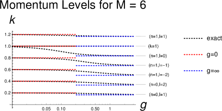
Figure 6: lowest seven momentum levels of Winter model, containing the first resonance, for $M=6$. The black dotted lines represent the exact levels, the red dotted lines the free limit ($g\to 0$) and the blue dotted lines the strong-coupling limit ($g\to\infty$). The degeneracy for $g\to 0$ of the flat level $k\equiv 1$ with the level just below it, namely the resonant level $k_{1}(g)$, is clearly visible. One may also notice that the level spacing at $g=0$, given by $\Delta k_{g=0}=1/(M-1)=0.2$, is larger than the spacing at $g=\infty$, which is equal to $\Delta k_{g=\infty}=1/M\simeq 0.167$. As in previous plot, the horizontal scale is logarithmic.

After excluding the flat levels, corresponding to the exceptional eigenfunctions in eq.(70), we observe that each momentum level $k$ is a strictly monotonically-decreasing function of $g$, with an upper horizontal asymptote given by the free limit $(g\to 0)$, represented by a dotted red line, and a lower horizontal asymptote given by the strong-coupling limit $(g\to\infty)$, represented by a dotted blue line.

By approaching a flat level from below, one encounters levels with total variation (the distance between the red line and the lower blue line) progressively bigger;

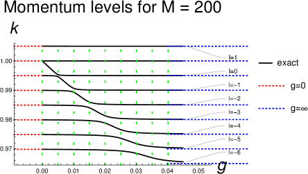
Figure 7: Momentum levels around the first or fundamental resonance $(n=1)$ for volume $M=200$. The black continuous lines represent the exact levels, the red dotted lines the free limit $g\to 0$ and the blue dotted lines the strong-coupling limit $g\to\infty$. The vertical light green dashed lines at $g=j/199\cong 0.005\times j$ $(j=0,1,2,3,\cdots)$ represent the coupling values where exactly-degenerate doublets $(j=0)$ or quasi-degenerate doublets $(j>0)$ occur in the spectrum.

the total variation of the level right above a flat one is instead extremely small. As already discussed, a flat level separates the levels having a resonant behavior (below it) from the levels not having such a behavior (above it).

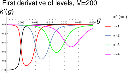
Figure 8: first derivatives of momentum levels $k$ as functions of the coupling $g$, namely $k^{\prime}(g)$, below and including the first or fundamental resonance $(n=1)$ for $M=200$. The vertical gray dashed lines at $g=j/199\cong 0.005\times j$ $(j=1,2,3,\cdots)$ represent the coupling values where quasi-degenerate doublets occur in the spectrum. Note that the intervals around the minima of $k^{\prime}(g)$ lie between two consecutive dashed lines.

A degeneracy for $g\to 0$ of the level $k\equiv 1$ with the level right below it (whose physical origin has been explained in sec. 6.2.2) is clearly seen in both figs. 5 and 6; A similar degeneracy of the level $k\equiv 1$ with the level right below it is also visible in fig. 6.

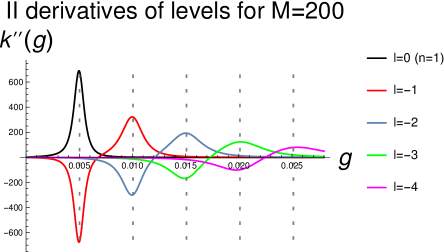
Figure 9: second derivatives of momentum levels $k$ as functions of the coupling $g$, $k^{\prime\prime}(g)$, below and including the first or fundamental resonance $(n=1)$ for $M=200$. The maxima and the minima of the function $k^{\prime\prime}(g)$ are quite close to the gray vertical dashed lines.

Figure 10: level spacing $\Delta k$ (difference between two contiguous momenta) as function of the coupling $g$, $\Delta k=\Delta k(g)$, for the levels below and including the first or fundamental resonance $(n=1)$ for $M=200$. The minima of $\Delta k(g)$ occur at $g\approx g_{j}\cong 0.005\times j$, $j=0,1,2,3,\cdots$, pretty close to the vertical gray dashed lines. By increasing $j$, the minima get less pronounced.

In fig. 7 we plot the momentum levels around the first or fundamental resonance $(n=1)$ in the large-volume case $M=200$. We notice that the resonant level $l=0$ (the level right below the flat one $k\equiv 1$) goes down roughly in a linear way with the coupling from the free-theory point $g=0$ (where it is degenerate with $k\equiv 1$, as we have already seen in the small-$M$ cases above) up to

$$g\,\approx\,g_{1}\,\equiv\,\frac{1}{N}\,\cong\,0.005\qquad(N=199);$$ (93)

where it shows a sharp variation of its first derivative — a quick increase up to zero; this phenomenon is also clearly seen both in figs. 8 and 9. For $g\raisebox{-3.0pt}{$\>\stackrel{{\scriptstyle>}}{{\scriptstyle\sim}}\>$}g_{1}$, this level $(l=0)$ is roughly constant, having already reached basically its infinite-coupling limit.

In general, the levels with $l<0$ (below the resonant one) are pretty flat for very small and very large couplings and show a rather sharp transition at $g=\mathcal{O}(1/N)$, when they substantially go from their respective free-theory values down to their infinite-coupling values. The $l=-1$ level, for example, is basically constant from $g=0$ up to $g\approx g_{1}$, where it shows a sharp decrease of its first derivative. In the coupling interval

$$g_{1}\,\,\raisebox{-3.0pt}{$\>\stackrel{{\scriptstyle<}}{{\scriptstyle\sim}}\>$}\,\,g\,\,\raisebox{-3.0pt}{$\>\stackrel{{\scriptstyle<}}{{\scriptstyle\sim}}\>$}\,\,g_{2}\,\equiv\,\frac{2}{N}\,\cong\,0.01,$$ (94)

this level goes down linearly with $g$. At $g\approx g_{2}$, it shows a sharp increase of its first derivative up to zero and finally, for $g\raisebox{-3.0pt}{$\>\stackrel{{\scriptstyle>}}{{\scriptstyle\sim}}\>$}g_{2}$, it is roughly constant, having basically reached its infinite-coupling limit. In general, the non-resonant level of index $l=-1,-2,-3,\cdots$ is constant from $g=0$ up to roughly

$$g_{|l|}\,\equiv\,\frac{|l|}{N}\,\cong\,0.005\times|l|,$$ (95)

where it shows a sharp decrease of its first derivative. Then, in the coupling interval

$$g_{|l|}\,\,\raisebox{-3.0pt}{$\>\stackrel{{\scriptstyle<}}{{\scriptstyle\sim}}\>$}\,\,g\,\,\raisebox{-3.0pt}{$\>\stackrel{{\scriptstyle<}}{{\scriptstyle\sim}}\>$}\,\,g_{|l|+1},$$ (96)

the level goes down roughly linearly with $g$. For $g\approx g_{|l|+1}$, it shows a sharp increase of its first derivative up to zero and for larger couplings it is basically flat. In general, by going away from a resonance level $(l=0)$ by taking $l=-1,-2,-3,-4,\cdots$, the above resonance behavior is softened.

Since the transition regions of different $l$ levels are shifted with respect to each other, for values of the coupling

$$g\,\approx\,g_{j}\,\equiv\,\frac{j}{N}\,\cong\,5\times 10^{-3}\times j;\qquad j=1,2,3,\cdots;$$ (97)

two black curves almost get in touch in fig. 7, implying that the corresponding doublet is quasi degenerate. The coupling values $g_{j}$ correspond to the vertical green dashed lines in figs. 7$-$10.

For the exceptional values of the coupling $g=g_{j}$ (eq.(97)), the first resonance of the infinite-volume model corresponds to the quasi-degenerate doublet having momenta, in the free limit $g\to 0$, given by $1-(j-1)/N$ and $1-j/N$. Note that the distance between the quasi-degenerate levels rapidly grows with $j$, so that this approximate degeneracy is barely visible for, let’s say, $j=\mathcal{O}(5)$.

Between the first two vertical green dashed lines in fig. 7, i.e. in the coupling range

$$0\,\,\raisebox{-3.0pt}{$\>\stackrel{{\scriptstyle<}}{{\scriptstyle\sim}}\>$}\,\,g\,\,\raisebox{-3.0pt}{$\>\stackrel{{\scriptstyle<}}{{\scriptstyle\sim}}\>$}\,\,g_{1},$$ (98)

there are three levels — rather than two as in general — in the momentum interval

$$0.995\,\,\raisebox{-3.0pt}{$\>\stackrel{{\scriptstyle<}}{{\scriptstyle\sim}}\>$}\,\,k\,\,\raisebox{-3.0pt}{$\>\stackrel{{\scriptstyle<}}{{\scriptstyle\sim}}\>$}\,\,1,$$ (99)

of width

$$\Delta k\,\simeq\,5\times 10^{-3}\,\simeq\,\frac{1}{N}\,\simeq\,\frac{1}{N+1}.$$ (100)

So long as $j=1,2,3,\cdots$ is not too large, this ”compression” of three levels also occurs in the coupling intervals

$$g_{j}\,\,\,\raisebox{-3.0pt}{$\>\stackrel{{\scriptstyle<}}{{\scriptstyle\sim}}\>$}\,\,\,g\,\,\,\raisebox{-3.0pt}{$\>\stackrel{{\scriptstyle<}}{{\scriptstyle\sim}}\>$}\,\,\,g_{j+1}.$$ (101)

For large $j$, i.e. for large values of the coupling $g$ compared to $1/N$, a resonance corresponds to a mild compression of many momentum lines.

We may summarize the above findings by saying that, for the exceptional values of the coupling $g=g_{j}$ given by eq.(97), the fundamental resonance of the usual Winter model corresponds, in the finite-volume case, to a quasi-degenerate doublet. For generic values of the coupling, the resonance corresponds instead to a compression of three lines in the typical spacing between two of them

$$\Delta k\,\approx\,\frac{1}{N}\,\approx\,\frac{1}{N+1};$$ (102)

For larger values of the coupling, i.e. for large $j$, the resonance corresponds to a mild compression of many levels. As in the small-volume cases considered above, only the levels below the flat one $k\equiv 1$ exhibit a resonant behavior; the levels above the latter (we have plotted just one of them in fig. 7) do not ”see” the resonance and are approximately constant in $g$.

6.3 Normal Eigenfunctions

As already discussed, by squeezing the system, the continuous spectrum of usual Winter model turns into a discrete one, with normal eigenfunctions, as functions of the momentum $k$ (solution of eq.(75)), given by:

$$\psi(k;\,x)\,=\,\mathcal{N}_{N}(k)\Big{\{}\theta(\pi-x)\sin(\pi Nk)\sin(kx)\,+\,\theta(x-\pi)\sin(\pi k)\sin\big{[}k(L-x)\big{]}\Big{\}};$$ (103)

where $\theta(z)\equiv 1$ for $z>0$ and zero otherwise is the Heaviside unit step function. As already defined, $N$ is the length, divided by $\pi$, of the segment $[\pi,L]$, i.e. the length of the large cavity $[\pi,L]$ to which the small cavity $[0,\pi]$ is coupled ($g\neq 0$). The normalization constant has the explicit expression:

$$\mathcal{N}_{N}(k)\,\equiv\,\Bigg{\{}\sin^{2}(\pi Nk)\left[\frac{\pi}{2}-\frac{\sin(2\pi k)}{4k}\right]\,+\,\sin^{2}(\pi k)\left[\frac{\pi N}{2}-\frac{\sin(2\pi Nk)}{4k}\right]\Bigg{\}}^{-1/2}.$$ (104)

In order to investigate resonant effects, it is convenient to rewrite the above eigenfunctions, as in the infinite-volume case [6], in terms of an amplitude and a phase:

$$\psi(k;x)\,=\,{\mathcal{C}_{N}(k)}\Big{\{}A_{N}(k)\,\theta(\pi-x)\,\sin(kx)\,+\,\theta(x-\pi)\,\sin\big{[}kx\,+\,\delta_{N}(k)\big{]}\Big{\}};$$ (105)

where:

1. $A_{N}(k)$ is the ratio of the inside amplitude $(0\leq x\leq\pi)$ over the outside one $(\pi\leq x\leq L)$,

   $$A_{N}(k)\,=\,\left|D_{N}(k)\right|;$$ (106)

   where (see fig. 11):

   $$\qquad D_{N}(k)\,\equiv\,\frac{\sin(\pi Nk)}{\sin(\pi k)};\qquad\qquad k\,\notin\,{\mathbb{Z}}.$$ (107)

   Note that, for odd $N$ ($M=N+1$ even), the function $D_{N}(k)$ is the Dirichlet’s Kernel of Fourier series theory.

2. $\delta_{N}(k)$ is the relative phase of the outside amplitude with respect to the inside one (see fig. 12),

   $$\delta_{N}(k)\,\equiv\,\arctan\left\{-\,\frac{\sin(\pi k)\cos[\pi(N+1)k]}{\sin(\pi Nk)};\,\,\frac{\sin(\pi k)\sin\left[\pi(N+1)k\right]}{\sin(\pi Nk)}\right\}.$$ (108)

   The two-argument arctangent function $\arctan(x,y)$ is a specification of $\arctan(y/x)$ which also takes into account in which quadrant the point $(x,y)$ lies in.

3. ${\mathcal{C}_{N}(k)}$ is an overall normalization constant,

   $${\mathcal{C}_{N}(k)}\,\equiv\,\Bigg{\{}D_{N}(k)^{2}\,\left[\frac{\pi}{2}-\frac{\sin(2\pi k)}{4k}\right]\,+\,\left[\frac{\pi N}{2}-\frac{\sin(2\pi Nk)}{4k}\right]\Bigg{\}}^{-1/2}.$$ (109)

The following remarks are in order:

1. Eq.(105) differs from eq.(103) by an overall sign only, namely

   $$\mathrm{sign}\left[D_{N}(k)\right],$$ (110)

   which, as well known, is physically irrelevant.

2. The appearance of the Dirichlet’s Kernel $D_{N}(k)$ in the finite-volume eigenfunctions (cfr. eq.(105)) suggests that the convergence of the latter to the corresponding infinite volume ones in the limit $N\to\infty$, will have to be intended as a weak one. This fact is a consequence of the rather ”hard” boundary conditions which we have chosen, namely reflecting ones, in comparison to the usual softer periodic boundary conditions.

Figure 11: Inside Amplitude $A_{N}$ as function of momentum $k$, $A_{N}=A_{N}(k)=\left|\sin(\pi Nk)\right|/\left|\sin(\pi k)\right|$, for a complete period, $0.5\leq k\leq 1.5$ (black continuous line) for $M=N+1=10$ . The red dotted line is the plot of the function $1/\left|\sin(\pi k)\right|$, namely the denominator of the Inside Amplitude, while the blue dotted line is the plot of the function $\left|\sin(\pi Nk)\right|$, the numerator of the Inside Amplitude.

Let us then discuss in the following sections the main properties of the Inside Amplitude and of the Phase Shift, as functions of the (still unrestricted) momentum $k$ .

6.3.1 Inside Amplitude as function of momentum

The Inside Amplitude $A_{N}$ as a function of the momentum $k$, $A_{N}=A_{N}(k)$, has the following properties:

1. Unitary period.

   The Inside Amplitude is periodic of period $T=1$,

   $$A_{N}(k+1)\,=\,A_{N}(k);\qquad k\,\in\,{\mathbb{R}}.$$ (111)

   The above equation trivially follows by taking the modulus on both sides of the equation (which is immediately verified)

   $$D_{N}(k+1)\,=\,(-1)^{N+1}\,D_{N}(k).$$ (112)

   Note that the function $D_{N}(k)$ is periodic with period $T=1$ for $N$ odd only, while it is periodic with period $T=2$ for $N$ even; in the latter case, $D_{N}(k)$ changes its sign for $k\to k+1$.

2. Principal maxima at integer momenta $k=1,2,3,\cdots$.

   The Inside Amplitude reaches a principal maximum when $k$ approaches an integer:

   $$\lim_{k\to n}A_{N}(k)\,=\,N;\qquad n\,=\,1,2,3,\cdots.$$ (113)

3. Zeroes for non-resonating momenta at zero coupling.

   For non-integer momenta of the form

   $$k\,=\,\frac{s}{N},$$ (114)

   i.e. with $s$ not an integer multiple of $N$,

   $$s\,\notin\,N{\mathbb{N}}_{+}\,\equiv\,\big{\{}N,\,2N,\,3N,\,\cdots\big{\}},$$ (115)

   or, even more explicitly,

   $$s\,=\,1,2,3,\cdots,N-1,N+1,\cdots,2N-1,2N+1,\cdots,$$ (116)

   the Inside Amplitude exactly vanishes:

   $$A_{N}\left(\frac{s}{N}\right)\,=\,0.$$ (117)

   That occurs because the numerator on the r.h.s. of the defining eq.(107) vanishes, while the denominator does not.

4. Local maxima in the midpoints of non-resonating momenta for $g\to 0$.

   By looking at fig. 11, we see that the local maxima of the Inside Amplitude are roughly in the middle of a pair of adjacent zeroes and are close to the maxima of its numerator, namely the function $|\sin(\pi Nk)|$. The latter lie at

   $$k\,=\,\left(u+\frac{1}{2}\right)\frac{1}{N};$$ (118)

   where $u$ is any signed integer,

   $$u\,=\,\cdots,\,-2,\,-1,\,0,\,1,\,2,\,3,\,\cdots.$$ (119)

   Actually, by looking carefully at fig. 11, we see that the maxima of $|\sin(\pi Nk)|$ closest to the point $k=1$, namely the points

   $$k\,=\,1\,\pm\,\frac{1}{2N}$$ (120)

   do not correspond to any maxima of the Inside Amplitude and have therefore to be excluded. Since $A_{N}(k)$ is periodic of period $T=1$, the above points are equivalent to the points

   $$k\,=\,\pm\,\frac{1}{2N},$$ (121)

   obtained by taking $u=0$ and $u=-1$ in eq.(118) respectively.

   The above rule to find the local maxima of the Inside Amplitude $A_{N}(k)$ can be analytically justified as follows. In the Large-Volume or Quasi-Continuum case, $N\gg 1$, the numerator of the Inside Amplitude, $|\sin(\pi Nk)|$, is rapidly varying with $k$, while the denominator, $|\sin(\pi k)|$ is slowly varying, as the factor $N$ is missing in the latter case. That implies that, in a small momentum interval $\delta k\ll 1$, one can consider the denominator as a constant and vary the numerator only. Therefore the local maxima of the Inside Amplitude are approximately at the momenta $k$ where $\sin(\pi Nk)$ is equal to $\pm 1$, i.e. at the points specified by eq.(118), where the index $u$ is any signed integer different from $0$ and $-1$.

   It is convenient to re-express the above result by explicitly taking into account the periodicity of $A_{N}(k)$. By means of the euclidean division of the index $s$ by $N$, one can write:

   $$s\,=\,nN\,+\,h,$$ (122)

   where

   $$n\,=\,\cdots,\,-2,\,-1,\,0,\,1,\,2,\,3,\,\cdots$$ (123)

   is the quotient and $h$, taken in the range

   $$\frac{N}{2}\,<\,h\,\leq\,\frac{N}{2};\qquad h\,\neq\,0;$$ (124)

   is the remainder. The non-resonating momentum in eq.(114) can then be written

   $$k\,=\,n\,+\,\frac{h}{N}.$$ (125)

   A local maximum of the Inside Amplitude is therefore at

   $$k\,\simeq\,n\,+\,\frac{h+1/2}{N};\qquad h\,\in\,{\mathbb{Z}}\setminus\left\{0,-1\right\}.$$ (126)

   On the above points, the Inside Amplitude takes the approximate values

   $$\frac{A_{N}\big{[}k\,=\,n+(h+1/2)/N\big{]}}{N}\,\simeq\,\frac{1}{\pi\,|h+1/2|}.$$ (127)

   The highest peak are

   $$\frac{1}{\pi\,|h+1/2|}\,\simeq\,0.212,\,\,0.127,\,\,0.0909,\,\,0.0707,\,\,0.0579,$$ (128)

   for

   $$h\,=\,1,\,\,2,\,\,3,\,\,4,\,\,5\qquad\mathrm{or}\qquad h\,=\,-2,\,\,-3,\,\,-4,\,\,-5,\,\,-6,$$ (129)

   respectively. As we see from the above formulae, the highest peak after the principal one $A_{N}(k=\mathrm{integer})=N$ is reached for $h=1$ (or $h=-2$) and is roughly $21\%$ of its value.

5. Unitary value in the large-coupling limit.

   For non-integer momenta of the form

   $$k\,=\,\frac{u}{N+1},$$ (130)

   with $u$ any integer not multiple of $N+1$,

   $$u\,\in\,{\mathbb{Z}}\,\setminus\,(N+1)\,{\mathbb{Z}},$$ (131)

   the Inside-Amplitude equals exactly one:

   $$A_{N}\left(\frac{u}{N+1}\right)\,=\,1.$$ (132)

   The above equation follows immediately from

   $$D_{N}\left(\frac{u}{N+1}\right)\,=\,\pm\,1.$$ (133)

   By means of the euclidean division of $u$ by $N+1$, the momentum $k$ in eq.(130) can be written

   $$k\,=\,n\,+\,\frac{l}{N+1},$$ (134)

   where

   $$n\,=\,\cdots,\,-2,\,-1,\,0,\,1,\,2,\,3,\,\cdots\quad\mathrm{and}\qquad\frac{N+1}{2}\,<\,l\,\leq\,\frac{N+1}{2}.$$ (135)

   Eq.(132) can be rewritten as

   $$A_{N}\left(n+\frac{l}{N+1}\right)\,=\,1.$$ (136)

   In the large-coupling limit, the ratio of the inside amplitude over the outside one goes to one, i.e. the amplitude is equal in both cavities. That is expected according to the fact that the potential barrier vanishes for $g\to\infty$.

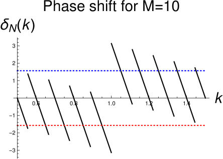
Figure 12: Phase Shift $\delta_{N}$ as function of the momentum $k$, $\delta_{N}=\delta_{N}(k)$ (black continuous line), in the period $0.5\leq k\leq 1.5$, for $M=10$. The blue/red dotted horizontal lines are the constant phases $\pm\pi/2$ respectively. The $2\pi$-discontinuity at $k=1$, together with the $\pi$-discontinuities at $k=1+l/N\simeq 1+0.11\times l$ $(l\neq 0)$, are clearly visible (see text).

6.3.2 Phase Shift as function of momentum

The Phase Shift $\delta_{N}$, as a function of the momentum $k$, $\delta_{N}=\delta_{N}(k)$ (eq.(108)), has the following properties (see fig. 12):

1. Unitary Period.

   The Phase Shift is periodic of period $T=1$, for both $N$ odd and $N$ even:

   $$\delta_{N}(k+1)\,=\,\delta_{N}(k)\qquad k\,\in\,{\mathbb{R}}.$$ (137)

2. Jump equal to $2\pi$ at integer momenta.

   With the following range of the two-argument arctangent,

   $$-\,\pi\,<\,\arctan(x,y)\,\leq\,\pi,$$ (138)

   i.e. with the discontinuity along the negative axis, the phase $\delta_{N}(k)$ has a jump (i.e. a finite discontinuity) equal to $2\pi$ whenever the momentum $k$ is an integer,

   $$k\,=\,n=1,2,3,\cdots.$$ (139)

   That is because the first argument of the arctangent is negative in a neighborhood of $k=n$, while the second one changes its sign by crossing the point $k=n$.

3. Jump of $\pi$ at non-resonating momenta for $g\to 0$.

   The phase $\delta_{N}(k)$ has a jump equal to $\pi$ at non-integer momentum of the form

   $$k\,=\,\frac{s}{N};$$ (140)

   i.e. when $s$ is not a multiple of $N$,

   $$s\,\notin\,N\,{\mathbb{N}}_{+}\,\equiv\,N\left\{1,2,3,\cdots\ \right\}\,\equiv\,\left\{N,2N,3N,\cdots\ \right\}.$$ (141)

   That is because because the function $\sin(\pi Nk)$, appearing in both arguments of the arctangent function (cfr. eq.(108)), changes its sign by crossing a momentum of the form (140).

4. Resonant behavior in the midpoints of non-resonant momenta for $g\to 0$.

   In terms of the standard arctangent function (periodic of period $\pi$ rather than $2\pi$ as the two-argument arctangent), the phase shift has the simple expression

   $$\delta_{N}(k)\,=\,-\,\pi(N+1)\,k\qquad(\mathrm{mod}\,\pi).$$ (142)

   According to the above formula, the phase passes through the resonant value $\pi/2$ (modulo $\pi$) whenever

   $$k\,=\,n+\frac{h+1/2}{N+1}\,\simeq\,n+\frac{h+1/2}{N}\qquad(N\gg 1).$$ (143)

   For $n=1$ and $h=1$, for example, a resonance occurs for $k\simeq 1+1.5/N$. Therefore, for large $N$, the phase shift passes through $\pi/2$ (modulo $\pi$) when the Inside Amplitude reaches a maximum (cfr eq.(126)).

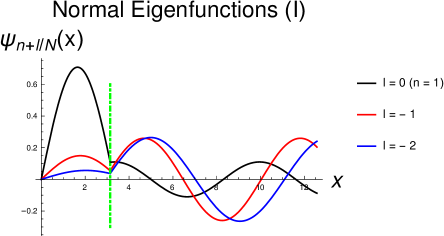
Figure 13: plots of normal eigenfunctions $\Psi_{n+l/N}(g;x)$ in the case of the rather small coupling $g=0.05$ and $N=9$. The black continuous line represents the first resonance, $n=1,l=0$; the red continuous line the level right below it, $n=1,l=-1$; finally, the blue continuous line is level $l=-2$. A thick dot-dashed green vertical line indicates the point $x=\pi$, the support of the $\delta$-function potential.

6.3.3 Normal Eigenfunctions for different couplings

The normal eigenfunctions, as functions of the integer index $s=1,2,3,\cdots$ and of the coupling $g$, are simply obtained by substituting, inside eq.(103) or (105), the independent momentum $k$ with the general solution of eq.(75):

$$\Psi_{s/N}(g;\,x)\,\equiv\,\psi\left[k\mapsto k_{s/N}(g);\,x\right];\qquad s=1,2,3,\cdots.$$ (144)

In order to simplify the notation, the explicit dependence on the coupling $g$ in the eigenfunctions will often be omitted, so that the latter will be written simply $\Psi_{s/N}(x)$.

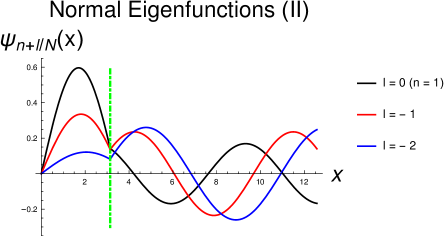
Figure 14: plots of normal eigenfunctions $\Psi_{n+l/N}(x)$ for $g=0.1$ and $N=9$. As in the previous plot, the black continuous line is the first resonance, $l=0$, the red continuous line the level $l=-1$ and the blue continuous line the level $l=-2$.

In figs. 13$-$15 we plot the eigenfunctions of the first resonance, $n=1$, $l=0$, and of the two levels right below it, $l=-1$ and $l=-2$, for different values of the coupling $g$ and for $N=9$. In fig. 13 the coupling chosen is rather small: $g=0.05$; the effective coupling $gN=0.45<1$ (see later). The $l=0$ eigenfunction (the black line) exhibits a rather marked resonance behavior, as its amplitude inside the small cavity is $6\div 7$ larger than outside it (i.e. inside the large cavity); furthermore, the $l=0$ eigenfunction is by far the largest one inside the small cavity. The $l=-1$ eigenfunction (the red line) is smaller roughly by a factor two inside the small cavity than outside it, not showing therefore any resonant behavior. Note the (finite) discontinuity of the first derivatives of all the eigenfunctions at $x=\pi$.

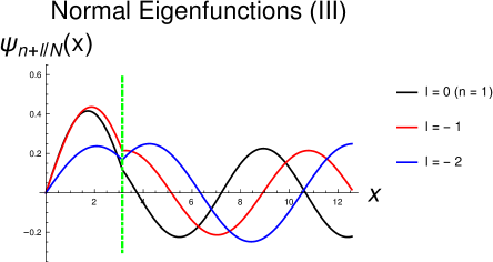
Figure 15: plots of normal eigenfunctions $\Psi_{n+l/N}(x)$ for the relatively large value of the coupling $g=0.2$ and $N=9$. As in previous plots, the black continuous line represents the first resonance, $n=1,l=0$, the red continuous line the level $l=-1$ and the blue continuous line the level $l=-2$.

In fig. 14 we have taken $g=0.1$, i.e. we have increased the coupling by a factor two with respect to the previous plot; the effective coupling $gN=0.9$, i.e. it is close to unity. The $l=0$ eigenfunction has a less marked resonance behavior compared to the previous plot, as it is larger by a $3\div 4$ factor only inside the small cavity than outside it; however, it is still the largest one inside the small cavity. Contrary to previous plot, the $l=-1$ eigenfunction is (slightly) larger inside the small cavity than outside it, showing therefore a mild resonant behavior. As in the previous plot, the $l=-2$ eigenfunction is still substantially smaller inside the small cavity than outside it, indicating the absence of any resonating behavior.

In fig. 15 the coupling has been increased by a further factor two: $g=0.2$; the effective coupling $gN=1.8$, i.e. it is substantially larger than unity. There is still an overall, though modest, resonant behavior. The main different with respect to the previous plots is that the $l=-1$ eigenfunction is (a bit) larger than the resonant one ($l=0$) inside the small cavity; the resonant behavior is ”transferred” from the level $l=0$ to the level $l=-1$. Furthermore, contrary to previous plots, the $l=-2$ eigenfunction is (slightly) larger inside the small cavity than outside it.

6.3.4 Inside Amplitude as function of the coupling

In order to understand the resonance phenomena occurring in the spectrum of finite-volume Winter model, let us consider in this section the Inside Amplitude $A_{N}$ as a function of the coupling $g$, which is our ”tuning” or ”detuning” parameter. The desired function is simply obtained by means of the replacement

$$k\,\mapsto\,k_{s/N}(g)$$ (145)

inside the function $A_{N}(k)$, giving rise to

$$A_{s/N}(g)\,\equiv\,A_{N}\left[k_{s/N}(g)\right];\qquad s=1,2,3,\cdots;\quad k>0.$$ (146)

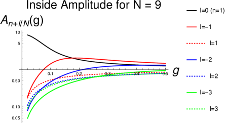
Figure 16: Inside Amplitude $A$ as a function of the coupling $g$ for various levels around and including the first resonance, $A=A_{n+l/N}(g)$, in the weak-coupling region $0.02\leq g\leq 0.5$ (which is the relevant one in the study of resonances) for $N=9$. The vertical scale — that of the Amplitude — is logarithmic, while the horizontal one — that of the coupling — is linear.

In fig. 16 the Inside Amplitude $A_{n+l/N}(g)$ for the first resonance, $n=1,\,l=0$, is plotted as a black continuous line. We see that $A_{1}(g)$ is the largest amplitude in the interval ranging from the free-theory point $g=0$, where

$$A_{1}(g=0)\,=\,N\,=\,9\,\gg\,1,$$ (147)

up to the critical value of the coupling

$$g\,=\,\bar{g}_{cr}\,=\,0.176\,\approx\,\frac{3}{2N}\,=\,0.167,$$ (148)

where it is surpassed by the $l=-1$ level (the red continuous line). At the critical point both Amplitudes have roughly a factor two enhancement,

$$A_{1}\left(\bar{g}_{cr}\right)\,=\,A_{1-1/N}\left(\bar{g}_{cr}\right)\,=\,2.03.$$ (149)

As already seen in the previous section, by increasing the coupling above $\bar{g}_{cr}$, the resonant behavior is transferred from the level $l=0$ down to the level right below it, namely the level $l=-1$. Actually, the $l=-1$ Inside Amplitude has a maximum at a value of the coupling a bit larger than $\bar{g}_{cr}$, namely at

$$\bar{g}_{l=-1}\,=\,0.187,$$ (150)

where it is slightly greater than at $\bar{g}_{cr}$:

$$A_{1-1/N}\left(\bar{g}_{l=-1}\right)\,=\,2.04.$$ (151)

The $l=-2$ Inside Amplitude (the continuous blue line) has a rather flat maximum at

$$\bar{g}_{l=-2}\,=\,0.461,$$ (152)

where it has a quite modest $30\%$ enhancement:

$$A_{1-2/N}\left(\bar{g}_{l=-2}\right)\,=\,1.31.$$ (153)

Finally, the $l=-3$ Inside Amplitude (the continuous green line) has a really flat maximum at

$$\bar{g}_{l=-3}\,=\,1.267,$$ (154)

where it has basically no enhancement,

$$A_{1-3/N}\left(\bar{g}_{l=-3}\right)\,=\,1.07.$$ (155)

Due to the large values of $\bar{g}_{l}$ found in the cases $l=-2$ and $l=-3$, one can reasonably state that these maxima cannot be described in perturbation theory. Finally, let us note that the Inside Amplitudes of the levels with $l>0$ (the dotted lines of various colors) never become larger than one, in complete agreement with the fact that they never resonate in the repulsive case $(g>0)$.

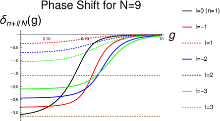
Figure 17: Phase Shift $\delta$ of the outside amplitude with respect to the inside one as a function of the coupling $g$, $\delta=\delta_{s/N}(g)$, for the levels close to the first resonance ($s=N$ or, equivalently $n=1$ and $l=0$), for a wide range of $g$, for $N=9$. The horizontal dotted brown lines denote the phases $-\pi/2$ and $-\pi$. The horizontal scale (that of the coupling $g$) is logarithmic while the vertical scale (that of the phase $\delta$) is linear.

6.3.5 Phase Shift as a function of the coupling

In this section we study the phase shift $\delta$ as a function of the coupling $g$,

$$\delta_{s/N}(g)\,\equiv\,\delta_{N}\left[k_{s/N}(g)\right];$$ (156)

where

$$s=1,2,3,\cdots,N-1,N,N+1,\cdots;\qquad k\,\in\,{\mathbb{R}}^{+}.$$ (157)

We consider the levels close to the first resonance both in figs. 17 and 18. As well known from scattering theory, an eigenfunction with a momentum $k=s/N+\mathcal{O}(g)$ exhibits a resonant behavior at a value of the coupling $g_{res}$ where its phase passes through $\pi/2$ (modulo $\pi$),

$$\delta_{s/M}\left(g=g_{res}\right)\,=\,\frac{\pi}{2}\qquad(\mathrm{mod}\,\pi),$$ (158)

with a large first derivative,

$$\frac{d\delta_{s/M}}{dg}\left(g_{res}\right)\,\gg\,1.$$ (159)

By looking at figs. 17 and 18, we see that the continuous black curve, representing the phase shift of the first resonance, $n=1$, $l=0$, crosses the upper brown dotted line $-\pi/2$, i.e. resonates, at

$$g\,=\,\hat{g}_{l=0}\,=\,0.0518\,\approx\,\frac{1}{2N}\,=\,0.556,$$ (160)

where the Inside Amplitude is large and $\mathcal{O}(N)$,

$$A_{1}\left(\hat{g}_{l=0}\right)\,=\,6.31.$$ (161)

The continuous red curve $l=-1$ intersects the brown line $-\pi/2$, i.e. resonates, at

$$\hat{g}_{l=-1}\,=\,0.152\,\approx\,\frac{3}{2N}\,=\,0.167,$$ (162)

a coupling value which is not far from the peak of the corresponding Inside Amplitude, $\bar{g}_{l=-1}\,=\,0.187$. On the contrary, the continuous blue line $l=-2$ intersects the upper brown line at

$$g\,=\,\hat{g}_{l=-2}\,=\,0.212,$$ (163)

a value of the coupling quite far from the maximum of the corresponding Inside Amplitude, $\bar{g}_{l=-2}=0.461$. Finally, the continuous green line, representing the Phase Shift of the level $l=-3$, crosses the brown line close to the intersection point of the $l=-2$ level. This sort of approximate degeneracy may be interpreted by saying that, by taking $l\leq-2$, we enter, as far as resonance dynamics is concerned, a strong-coupling region, where usual perturbation theory does not work (the effective coupling $N\hat{g}_{l=-2}\approx 2$). In order to study these $l$ values in perturbation theory, one has to go to larger values of $N$.

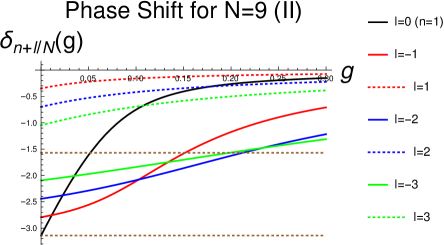
Figure 18: Phase Shift $\delta=\delta_{s/N}(g)$, for the levels close to the first resonance ($n=1,\,l=0$), for small values of $g$ and for $N=9$. In this plot both scales are linear.

The Phase Shifts of the levels with $l>0$ (the dotted lines of various colors) have a very small variation with $g$ and, in particular, they never cross the brown line $-\pi/2$, implying the absence of any resonant behavior for $g>0$, in agreement with the results obtained for the Inside Amplitude (see previous section).

7 Ordinary Perturbation Theory

In the analytic calculations, we always assume

$$0\,<\,g\,\ll\,1,$$ (164)

i.e. a weakly-repulsive interaction, in order to use perturbation theory in $g$ and avoid bound-state effects. The momentum on the r.h.s. of eq.(87) can be considered the zero order term of a perturbative expansion in the coupling $g$. One has to distinguish between:

1. Resonant case, when $s$ is an integer multiple of $N$,

   $$s\,=\,n\,N;\qquad n=1,2,3,\cdots,$$ (165)

   so that the unperturbed momentum is integer,

   $$k^{(0)}\,=\,n;$$ (166)

2. Non-resonant case, when $s$ is not multiple of $N$, i.e. the fraction on the r.h.s. of eq.(87) is not apparent; the unperturbed momentum is written in this case

   $$k^{(0)}\,=\,n\,+\,\frac{l}{N};$$ (167)

   with

   $$-\,\frac{N}{2}\,<\,l\,\leq\,\frac{N}{2};\qquad l\,\neq\,0.$$ (168)

The perturbative expansion of the constant levels $p_{n}\equiv n$ is of course trivial, as these levels do not depend on $g$.

7.1 Resonant case

In the resonant case, the expansion is written

$$\qquad\qquad k_{n}\,=\,k_{n}(g)\,=\,n\left(1\,+\,\sum_{i=1}^{\infty}g^{i}\,c_{n}^{(i)}\right);\qquad n=1,2,3,\cdots;$$ (169)

As already discussed, we label the momentum levels by means of their limiting values for $g\to 0$:

$$k_{n}(g=0)\,=\,n.$$ (170)

By recursively solving in $g$ the momentum eigenvalue eq.(75), one obtains for the first few coefficients:

$$c^{(1)}_{n} = -\left(1\,+\,\frac{1}{N}\right);$$ (171)

$$c^{(2)}_{n} = +\left(1\,+\,\frac{1}{N}\right)^{2};$$

$$c^{(3)}_{n} = +\,\left(1+\frac{1}{N}\right)^{3}\left(\frac{\,\pi^{2}}{3}\,n^{2}N\,-\,1\right).$$ (172)

Let us comment on the above results. The resonances of the usual, infinite-volume model are related to the poles in the complex $k$-plane [3, 6]

$$k\,=\,\chi_{n}(g)\,=\,n\Big{(}1\,+\,g\,b^{(1)}_{n}\,+\,g^{2}\,b^{(2)}_{n}\,+\,\cdots\Big{)};$$ (173)

where

$$b^{(1)}_{n}\,=\,-\,1;\qquad b^{(2)}_{n}\,=\,1\,-\,i\pi n.$$ (174)

For $N\to\infty$, i.e. in the infinite-volume limit, the first-order coefficient $c^{(1)}_{n}=c^{(1)}_{n}(N)$ smoothly goes into the corresponding coefficient $b^{(1)}_{n}$ of the infinite-volume theory,

$$\lim_{N\to\infty}c^{(1)}_{n}\,=\,b^{(1)}_{n};$$ (175)

furthermore, $c^{(2)}_{n}$ goes into the real part of $b^{(2)}_{n}$,

$$\lim_{N\to\infty}c^{(2)}_{n}\,=\,\mathrm{Re}\,b^{(2)}_{n};$$ (176)

Surprises come at third order: by looking at the expression of the third-order coefficient $c^{(3)}_{n}$ above, we find a secular term proportional to $N$, giving a contribution to $k_{n}(g)$ of the form $g^{3}N$. By analyzing higher-order coefficients (which we have not displayed), we find that the occurrence of positive powers of $N$ in the coefficients $c^{(i)}_{n}$ is a general phenomenon: The term $g^{i}c_{n}^{(i)}$, for $i=3,4,5,\cdots$, contains monomials of the form

$$g^{2}(gN)^{i-2},\quad g^{3}(gN)^{i-3},\quad g^{4}(gN)^{i-4},\quad\cdots.$$ (177)

To have a convergent series, we have therefore to restrict the range of the perturbative expansion to the parameter-space region

$$0\,<\,g\,N\,\ll\,1,\qquad\mathrm{or\,\,equivalently}\qquad 0\,<\,g\,\ll\,\frac{1}{N}.$$ (178)

For small sizes of the larger cavity, let’s say $N=\mathcal{O}(1)$, the secular terms shown in (177) do not present any problem, as they do not lead to any substantial enhancement in the coefficients $c_{n}^{(i)}=c_{n}^{(i)}(N)$ entering the expansion of $k_{n}=k_{n}(g,N)$. On the contrary, for large $N$, the terms in (177) tend instead to spoil the convergence of the perturbative expansion. The occurrence of such secular terms in the momentum expansion implies in particular that we can no more take the infinite-volume limit $N\to\infty$ in a straightforward way, as we have made in the first-order and second-order cases.

In the very-small coupling region specified by the inequalities in (178), the allowed momentum

$$k_{n}(g)\,=\,n\,-\,g\,n\left(1+\frac{1}{N}\right)\,+\,\cdots$$ (179)

is very close to — slightly below — the exceptional, exactly-integer momentum

$$p_{n}\,\equiv\,n,$$ (180)

whose corresponding eigenfunction has been given in eq.(70). Their separation vanishes indeed in the free limit:

$$p_{n}\,-\,k_{n}(g)\,=\,g\,n\left(1+\frac{1}{N}\right)\,+\,\cdots.$$ (181)

The conclusion is that for very small couplings, $g\ll 1/N$, the quasi-degenerate doublet

$$\big{(}k_{n}(g),\,p_{n}\big{)}$$ (182)

corresponds to the $n^{\mathrm{t}h}$ resonance of the usual, infinite-volume model, for any $n=1,2,3,\cdots$. Ordinary perturbation theory therefore allows an analytic description of the exact double degeneracy for $g\to 0$, which we have observed in the plots of the exact levels in figs. 5$-$7 and in fig. 10.

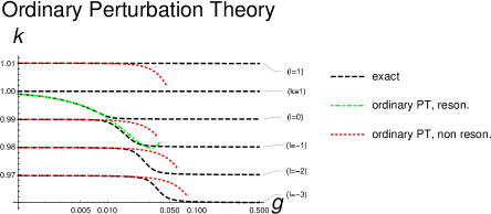
Figure 19: momentum levels around the first or fundamental resonance $(n=1)$ as functions of the coupling, $k=k(g)$, in the large-volume case $M=100$. The black dashed lines are the plots of the exact levels, the green dot-dashed line represents the ordinary perturbative formula for the resonant level ($l=0$), while the red lines are the plots of the perturbative formulae in the non-resonant cases ($l\neq 0$). The horizontal scale is logarithmic.

7.2 Non-resonant case

In the non-resonant case, the perturbative expansion of the momenta, according to eq.(89), is written:

$$\qquad\qquad\qquad k\,=\,k_{n+l/N}(g)\,=\,\left(n\,+\,\frac{l}{N}\right)\left(1\,+\,\sum_{i=1}^{\infty}g^{i}\,c^{\,(i)}_{n+l/N}\right)\qquad\qquad(l\neq 0).$$ (183)

As in the resonant case, the momentum levels, as functions of the coupling, are labeled by their limiting values for $g\to 0$:

$$k_{n+l/N}(g=0)\,=\,n\,+\,\frac{l}{N}.$$ (184)

The lowest-order coefficients of the perturbative expansion have the following explicit expressions:

$$c_{n+l/N}^{\,(1)} = -\,\frac{1}{N};$$ (185)

$$c_{n+l/N}^{\,(2)} = +\,\frac{\pi}{N}\left(n+\frac{l}{N}\right)\cot\left(\frac{\pi l}{N}\right)+\frac{1}{N^{2}};$$

$$c_{n+l/N}^{\,(3)} = -\,\frac{\pi^{2}}{N}\left(1-\frac{1}{N}\right)\left(n+\frac{l}{N}\right)^{2}\csc^{2}\left(\frac{\pi l}{N}\right)\,+$$

$$-\,\frac{3\pi}{N^{2}}\left(n+\frac{l}{N}\right)\cot\left(\frac{\pi l}{N}\right)+\frac{4\pi^{2}}{3N}\left(n+\frac{l}{N}\right)^{2}-\frac{1}{N^{3}};$$

where $\cot(x)$ and $\csc(x)$ are the cotangent and the cosecant of $x$ respectively. By expanding the above coefficients for large $N$, one obtains:

$$c_{n+l/N}^{\,(1)} = -\,\frac{1}{N};$$

$$c_{n+l/N}^{\,(2)} = +\,\frac{n}{l}\,+\,\frac{1}{N}\,+\,\mathcal{O}\left(\frac{1}{N^{2}}\right);$$

$$c_{n+l/N}^{\,(3)} = -\,\left(\frac{n}{l}\right)^{2}\,N\,+\,\frac{n\,(n-2l)}{l^{2}}\,+\,\frac{\pi^{2}\,n^{2}-n/l-1}{N}\,+\,\mathcal{O}\left(\frac{1}{N^{2}}\right).$$ (186)

In general, any additional power of the coupling $g$ brings, inside its corresponding coefficient, an additional power of $N$; The third-order coefficient, in particular, has a secular term linear in $N$, as in the resonant case.

7.3 Discussion

In fig. 19 we plot the exact momentum levels around the first resonance $(n=1)$ together with their ordinary perturbative expansions, for $M=100$. The dot-dashed green curve, representing the perturbative expansion of the first resonant level (the plot of eq.(169) with $n=1$ truncated at third order in $g$) is very close to the corresponding exact curve (the black dashed line) from $g=0$ up to $g\approx 10^{-2}$; around this point (as already seen in the previous $M=200$ plot, fig. 7), the exact curve basically reaches its lower asymptote, showing a quick and large variation of its first derivative and getting pretty close to the lower, non-resonating, curve $l=-1$. For values of the coupling in the region

$$10^{-2}\,\,\raisebox{-3.0pt}{$\>\stackrel{{\scriptstyle<}}{{\scriptstyle\sim}}\>$}\,\,g\,\,\raisebox{-3.0pt}{$\>\stackrel{{\scriptstyle<}}{{\scriptstyle\sim}}\>$}\,\,2\times 10^{-2},$$ (187)

the resonant perturbative curve is rather close to (a little above actually) the exact curve of the non-resonant level $l=-1$. Above $g\approx 2\times 10^{-2}$, the perturbative curve shows an unphysical rise and is no more able to describe any level. It is noticeable that a single perturbative formula (approximately) describes two distinct levels — rather than one — in two different coupling regions.

The plots of the perturbative expansions of the non-resonant levels for $l<0$ (the red dotted lines below the green dot-dashed line) remain close to the corresponding exact curves (black dashed lines) from $g=0$ up to the coupling region where the latter make a transition from the upper asymptote to the lower one. The perturbative curves are not able to correctly reproduce this transition, showing some sort of ”delay”. As in previous fig. 7, the exact curve of the non-resonant level $l=1$ (the level right above $k\equiv 1$) is pretty flat in all the coupling range; the corresponding perturbative curve (the red dotted line above the green dot-dashed line) is close to the exact one from $g=0$ up to approximately $g\approx 2\times 10^{-2}$, where it shows an unphysical decrease.

8 Resummed Perturbation Theory

The parameter-space region

$$g\,N\,\raisebox{-3.0pt}{$\>\stackrel{{\scriptstyle>}}{{\scriptstyle\sim}}\>$}\,1,$$ (188)

which is out of control with ordinary perturbation theory as we have seen in the previous section, can be studied by means of improved perturbative expansions, generated in the limit

$$g\,\to\,0^{+},\quad N\,\to\,+\,\infty\qquad\mathrm{with}\qquad\xi\,\equiv\,g\,N\,\to\,\mathrm{constant}.$$ (189)

As in the case of ordinary perturbation theory, we have to treat separately the resonant momenta and the non-resonant ones.

8.1 Resonant case

In the resonant case, the $k_{n}$’s are represented by function series of the form:

$$k_{n}\,=\,n\left(1\,+\,\sum_{i=1}^{\infty}g^{i}\,h_{n}^{(i)}(\xi)\right).$$ (190)

By means of standard multi-scale techniques [34], one obtains for the lowest-order functions:

$$h_{n}^{(1)}(\xi) = -\,1;$$

$$h_{n}^{(2)}(\xi) = -\,\nu\,\cot\left(\nu\,\xi\right)\,+\,1;$$ (191)

$$h_{n}^{(3)}(\xi) = +\,\nu^{3}\xi\cot^{3}\left(\nu\,\xi\right)\,-\,\nu^{2}(1+\xi)\,\cot^{2}\left(\nu\,\xi\right)\,+\,$$

$$+\,\nu\left(\nu^{2}\xi+3\right)\cot\left(\nu\,\xi\right)\,+\,\nu^{2}\left(\frac{1}{3}-\xi\right)\,-\,1;$$

where we have defined

$$\nu\,\equiv\,\pi\,n.$$ (192)

The functions $g^{i}h^{(i)}_{n}(\xi)$, $i>1$, have pole singularities whenever

$$nNg\,=\,j\,=\,1,2,3,\cdots.$$ (193)

For a given size of the large cavity, i.e. for given $N$, and for a given resonance, i.e. for given $n$, the functions $h^{(i)}_{n}(\xi)$ become singular when the coupling $g$ approaches one point of the sequence

$$g_{j}\,\equiv\,\frac{j}{n\,N};\qquad j\,=\,1,2,3,\cdots.$$ (194)

As we have seen in figs. 7$-$10, the points $g_{j}$ are the particular values of the coupling $g$ where the exact levels present a large variation of their first derivatives and quasi-degenerate doublets occur in the spectrum.

A physical argument about the origin of the $g_{j}$ singularities is the following. The eigenfunctions of a free particle in the $[0,\pi]$ box have exactly integer momenta:

$$k_{\,[0,\pi]\,\mathrm{box}}\,=\,n\,=\,1,2,3,\cdots.$$ (195)

As already discussed, by weakly-coupling such states to a continuum, the box becomes a resonant cavity and the above box momenta are subjected to a finite renormalization [3, 9] which, to first order in $g$, gives the resonant momenta (cfr. eq.(173))

$$\chi_{n}(g)\,\approx\,n\,-\,ng.$$ (196)

Now, if we couple the $[0,\pi]$ box to the large $[\pi,L]$ box, rather than to the half line $[\pi,\infty)$, we expect singularities to occur in the perturbative expansion of $k_{n}=k_{n}(g,\xi)$, whenever a resonant momentum $\chi_{n}(g)$ of the infinite-volume theory becomes equal to an allowed momentum of the particle in the large box, namely when

$$\chi_{n}(g)\,\approx\,n\,+\,\frac{l}{N}.$$ (197)

By replacing the explicit form of $\chi_{n}(g)$ given in eq.(196), we obtain the relation

$$nNg\,\approx\,-\,l.$$ (198)

If we now identify $j$ with $-l$, we obtain eq.(193).

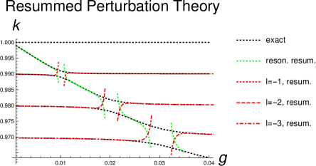
Figure 20: few momentum levels below the first or fundamental resonance $(n=1)$ for $M=100$. The black dotted lines are the plots of the exact levels, the green dotted line represents the resummed formula in the resonant case $(l=0)$, while the red lines represent the resummed formulae in the non-resonant cases $(l\neq 0)$. To be more specific, the red dotted line is the level $l=-1$, the red dashed line is the level $l=-2$ and the red dot-dashed line the level $l=-3$. The singularities of the resummed formulae at the points $g=g_{j}\equiv j/(nN)=j/99\cong 0.01\times j$, corresponding to quasi-degenerate doublets and large variations of their first derivatives, are clearly visible for $j=1,2,3$.

8.2 Non-resonant case

In the non-resonant case, the resummed expansion in the effective coupling $\xi$ for the quantized momentum $k_{n+l/N}\,=\,k_{n+l/N}(g,\xi)$ is written:

$$\qquad\qquad\qquad\qquad k_{n+l/N}\,=\,\left(n\,+\,\frac{l}{N}\right)\left(1\,+\,\sum_{i=2}^{\infty}g^{i}\,h^{(i)}_{n+l/N}(\xi)\right)\qquad\qquad(l\neq 0);$$ (199)

where:

$$h^{(2)}_{n+l/N}(\xi) = \frac{n}{l+n\,\xi}\,-\,\frac{1}{\xi};$$

$$h^{(3)}_{n+l/N}(\xi) = \frac{l\,n^{2}}{(l+n\,\xi)^{3}}\,-\,\frac{ln}{(l+n\,\xi)^{2}}\,-\,\frac{n}{l+n\,\xi}\,+\,\frac{1}{\xi}.$$ (200)

Figure 21: few momentum levels below the second or first-excited resonance $(n=2)$ for the case $M=100$. The plot scheme is the same as in previous figure 20, so we do not repeat its description. The singularities of the resummed formulae at $g=j/198\simeq 0.005\times j$, corresponding to quasi-degenerate doublets and large variations of their first derivative, are clearly visible for $j=1,2,3$.

The series begins at second order in $g$ because the term

$$\frac{l}{N}\,=\,\frac{g\,l}{\xi}$$ (201)

is already of first order and the perturbative expansion is supposed to be a small correction to the unperturbed result.

The momentum $k_{n+l/N}(g)$, as given by the r.h.s. of eq.(199) truncated at some order in $g$, is approximated by a sum of rational functions of the coupling $g$, i.e. at the end by a rational function of $g$, rather than by a polynomial in $g$, as in ordinary perturbation theory.

For a given size of the large cavity, i.e. for given $N$, and for a given state, i.e. for given $n$ and $l$, the functions $h^{(i)}_{n+l/N}$, describing the levels close to the $n^{\mathrm{th}}$ resonance, become singular when the coupling $g$ approaches the value

$$g\,=\,g_{-l}\,\equiv\,\frac{-\,l}{n\,N};\qquad l\,=\,\pm 1,\,\pm 2,\,\pm 3,\,\cdots.$$ (202)

In the repulsive case to which we restrict, $g>0$, the above singularity occurs for $l<0$ only, i.e. in the levels below the resonant one.

8.3 Discussion

In fig. 20 we compare the exact momentum levels below and including the first resonance $n=1$ (black dotted lines), with the corresponding resummed expansions (green dotted line and red lines).

Let’s discuss first the simpler non-resonant case. The resummed formula for the $l^{\mathrm{t}h}$ level given in eq.(199) (the red dotted, dashed and dot-dashed line for $l=-1,-2$ and $-3$ respectively) correctly reproduces the corresponding $l^{\mathrm{th}}$ level from $g=0$ almost up to its singularity, at

$$g_{|l|}\,=\,\frac{|l|}{99}\,\cong\,0.01\times|l|.$$ (203)

For example, the $l=-1$ resummed formula (the red dotted line) describes pretty well this level from $g=0$ almost up to its singularity, at $g_{1}\cong 0.01$. But what happens for larger, still perturbative, couplings? The problem is that the resummed formula in eq.(199) is not continuous at $g=g_{|l|}$, because it has a pole at this point. It is therefore not clear a priori which level this formula is going to describe beyond this singularity, if any. In particular, there is no reason to expect that this formula will still describe the $l^{\mathrm{th}}$ level after the singularity, i.e. for $g>g_{|l|}$. By looking at fig. 20, it is found that for couplings slightly above $g_{|l|}$ up to relatively large values of $g$, the $l^{\mathrm{th}}$ resummed curve reproduces quite accurately the next upper level, i.e. the level with index $l+1$. For example, if we fix the value $l=-1$ in eq.(199), we obtain a formula which reproduces the exact curve $l=-1$ below the singularity, at $g=g_{1}\cong 0.01$, and the resonant level $l=0$ above $g_{1}$. In general, therefore, a resummed formula for a non-resonant level describes two different momentum levels, in two different coupling regions.

Let’s now consider the effects of the resummation to all orders in $\xi$ of the perturbative series for a resonant level. The (truncated) function series on the r.h.s. of eq.(190) has a sequence of pole singularities located, in the case of the first resonance $n=1$ and volume $N=99$, at

$$\qquad\qquad\qquad\qquad g\,=\,g_{j}\,\equiv\,\frac{j}{n\,N}\,=\,\frac{j}{99}\,\cong\,0.01\times j;\qquad j=1,2,3,\cdots;\quad j\ll N.$$ (204)

As in the non-resonant case, the resummed formula in eq.(190) does not need to describe above each singularity, i.e. for $g>g_{j}$, the same level described below it, i.e. for $g<g_{j}$. By looking at fig. 20, it is found that the resummed formula for the first resonance (represented by the green dotted curve) reproduces pretty well, from $g=0$ up to almost its first singularity, at $g_{1}\simeq 0.01$, the exact level. Between the first and the second singularity, i.e. for values of the coupling $g$ in the interval

$$g_{1}\,\simeq\,0.01\,\,\raisebox{-3.0pt}{$\>\stackrel{{\scriptstyle<}}{{\scriptstyle\sim}}\>$}\,\,g\,\,\raisebox{-3.0pt}{$\>\stackrel{{\scriptstyle<}}{{\scriptstyle\sim}}\>$}\,\,g_{2}\,\simeq\,0.02,$$ (205)

the $n=1$ resummed formula describes the transition region of the level right below the resonant one, i.e. the non-resonant level with $l=-1$. In general, in the coupling region

$$g_{j}\,\,\raisebox{-3.0pt}{$\>\stackrel{{\scriptstyle<}}{{\scriptstyle\sim}}\>$}\,\,g\,\,\raisebox{-3.0pt}{$\>\stackrel{{\scriptstyle<}}{{\scriptstyle\sim}}\>$}\,\,g_{j+1},$$ (206)

the resummed formula for a resonant level describes the transition region of the non-resonant level with $l=-j$ (so long as we are in the weak-coupling regime of course). We find truly remarkable the fact that the resummed formula for the $n^{\mathrm{t}h}$ resonance describes the $n^{\mathrm{t}h}$ resonance level from $g=0$ almost up to $g_{1}$, i.e. basically its transition region, together with an entire sequence of non-resonant levels, in their respective transition regions.

In fig. 21 we compare the exact and resummed momentum levels below and including the second or first-excited resonance $n=2$. In agreement with the general formula in eq.(194), the resummed formulae are singular at

$$g\,=\,g_{j}\,=\,\frac{j}{2N}\,=\,\frac{j}{198};\qquad j=1,2,3,\cdots$$ (207)

As we have found in fig. 20 for the first resonance (as well as in the previous $M=200$ plots, cfr. fig. 7), the exact levels show at the points $g_{j}$ quasi-degenerate doublets and large variations of their first derivatives. In general, the plots for $n=2$ are very similar to the corresponding ones for the first resonance, so we do not repeat the discussion.

In fig. 22 we compare the momentum levels around the first resonance ($n=1$) computed with ordinary perturbation theory with the levels computed with resummed perturbation theory. In general, the resummed formulae work definitively better than the corresponding fixed-order ones. After excluding proper neighborhoods of the singularities at $g=g_{j}$ $(j=1,2,3,\dots)$ and proper matching, resummed perturbation theory correctly describes all the momentum levels so long as $g\ll 1$.

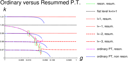
Figure 22: ordinary versus resummed perturbation-theory levels around the first resonance $n=1$. The magenta dot-dashed curve is the plot the resonant level computed in ordinary perturbation theory, while the dotted green line describes the same level in resummed perturbation theory. The red dotted, dashed and dot-dashed curves describe the non-resonant levels in resummed perturbation theory for $l=\pm 1$, $l=-2$ and $l=-3$ respectively, while the dotted blue lines describe the same levels in ordinary perturbation theory. The flat level $p_{1}\equiv 1$ (black dotted line), separating the non-resonating levels (above it) from the resonating ones (below it), is also shown for completeness. The horizontal scale is logarithmic.

9 Conclusions

We have computed the spectrum of Winter or $\delta$-shell model at finite volume both numerically and by means of perturbative methods. For very small repulsive couplings,

$$0\,<\,g\,\ll\,\frac{1}{N},$$ (208)

the resonance of order $n=1,2,3,\cdots$ of usual Winter model corresponds, in the finite-volume case, to a quasi-degenerate doublet with momenta

$$k_{n}(g)\,=\,n\,-\,g\,n\left(1+\frac{1}{N}\right)\,+\,\cdots\qquad\mathrm{and}\qquad p_{n}\,\equiv\,n.$$ (209)

The distance between these levels goes to zero linearly with the coupling:

$$p_{n}\,-\,k_{n}(g)\,=\,g\,n\left(1+\frac{1}{N}\right)\,+\,\cdots.$$ (210)

The physical origin of this degeneracy is related to the fact that, for very small couplings, a wavefunction with an integer momentum is, to a good approximation, an eigenfunction of both the small $[0,\pi]$ box and the large $[\pi,L]$ one. In more physical terms, for $g\to 0$, a particle with integer momentum can be entirely and permanently confined either in the small cavity or in the large one. This degeneracy is well described by ordinary perturbation theory.

In the large-volume cases,

$$N\,\gg\,1,$$ (211)

new approximate degeneracy’s occur in the spectrum. The exact momentum levels $k$ as functions of the coupling $g$, $k=k(g)$, show a large variation of their first derivatives and quasi-degenerate doublets occur in the spectrum, when

$$g\,\approx\,g_{j}\,\equiv\,\frac{j}{n\,N};\qquad j=1,2,3,\cdots.$$ (212)

For generic values of the coupling, of the order of the inverse of the system size,

$$g\,\approx\,\frac{1}{N}\,\ll\,1,$$ (213)

an infinite-volume resonance corresponds to the compression of three lines in the typical spacing between two of them and, by increasing further the coupling, to a mild compression of many lines, let’s say $h=4,5,\cdots$ lines in the typical spacing of $h-1$ lines (see fig. 10).

The perturbative expansion of the momentum spectrum of the finite-volume model contains secular terms, from third order in $g$ on, of the form

$$g^{i}\,N^{i-2},\quad g^{i}\,N^{i-3},\quad g^{i}\,N^{i-4},\quad\cdots\qquad(i=3,4,5,\cdots).$$ (214)

For large volumes, $N\gg 1$, these terms can be of order one (or bigger) even in the weak coupling regime $g\ll 1$, so they tend to spoil the convergence of the perturbative series. Not surprisingly, ordinary perturbation theory is completely unable to describe these approximate degeneracy’s of the spectrum. By resumming the perturbative series for the momenta $k=k(g,\xi)$ to all orders in the effective coupling

$$\xi\,\equiv\,g\,N\,=\,\mathcal{O}(1),$$ (215)

and to some (finite) order in $g\ll 1$, one obtains improved expansions presenting pole singularities at $g=g_{j}$. We may say that, in some sense, the resummed formulae ”see” the quasi-degeneracy points $g_{j}$. After the exclusion of small neighborhoods of the singular couplings $g_{j}$ and proper matching of the resummed levels with the exact ones, improved perturbation theory accurately describes the complete momentum spectrum. We can therefore claim that resummed perturbation theory provides a satisfactory analytic description of resonances at finite volume in the case of the Winter model.

As far as the physical relevance of Winter model at finite volume is concerned, we believe that this system can provide, as discussed in the Introduction, highly non-trivial checks of the general superposition principle of quantum mechanics. By means of spectral decomposition, one finds that the dynamics of a standard resonance is controlled by the interference of its energy eigenstates. In general, resonance dynamics at finite volume involves more complicated superpositions of energy eigenfunctions than at infinite volume, because of additional wave-reflection phenomena. Let us consider an initial wavefunction $\psi_{0}(x)$ with the particle inside the small cavity, where $\left|\psi_{0}\right|=\mathcal{O}(1)$. At a time

$$t\,\approx\,T\,\equiv\,\frac{L}{v},$$ (216)

where $L\gg 1$ is the large-cavity size and $v$ is the average particle velocity, the wavefunction completely spreads out in the large cavity, where it is consequently very small,

$$|\psi(T)|\,\approx\,\frac{1}{\sqrt{L}}\,\ll\,1.$$ (217)

Yet, because of coherence, by evolving the system by even larger times than $T$, recurrence will occur and the particle will be back in the small cavity with a probability close to one. Eventually, limited-decay phenomena may occur. If we approximate the $\delta$-function of Winter model Hamiltonian by means of a rectangular potential barrier, the finite-volume model can be physically realized by a quantum well. In this way, recurrence and limited-decay phenomena can be experimentally investigated.

Acknowledgments

I wish to thank D. Anselmi and M. Papinutto for discussions.

References

- [1] P. A. M. Dirac, ”The Principles of Quantum Mechanics”, Oxford University Press, Oxford OX2 6DP, Fourth Edition (1958).
- [2] T. D. Lee, ”Particle Physics and Introduction to Field Theory”, Harwood Academic Publishers, Third Printing, Revised and Updated First Edition (1988).
- [3] U. G. Aglietti and P. M. Santini, “Analysis of a Quantum Mechanical Model for Unstable Particles”, arXiv:1010.5926v2 [quant-ph] and references therein.
- [4] S. Flugge, ”Practical Quantum Mechanics”, Springer-Verlag, Berlin (1994), problem n. 27, ”Virtual levels”.
- [5] The classic references on the matrix are: R. Newton, ”Scattering of Waves and Particles”, Dover Publications, Inc. Mineola, New-York (2004); M. Goldberger and K. Watson, ”Collision Theory”, Dover Publications, Inc. Mineola, New-York (2002).
- [6] R. G. Winter, “Evolution of a Quasi-Stationary State”, Phys. Rev. 123, n. 4, pag. 1503 (1961).
- [7] K. Gottfried, ”Quantum Mechanics”, W. A. Benjamin (1966).
- [8] D. A. Dicus, W. W. Repko, R. F. Schwitters and T. M. Tinsley, ”Time Development of a Quasi-Stationary State”, Phys. Rev. A 65, 032116 (2002).
- [9] U. G. Aglietti and P. M. Santini, “Renormalization in the Winter Model”, Phys. Rev. A 89, 022111 (2014).
- [10] U. G. Aglietti and P. M. Santini, ”Geometry of Winter Model”, J. Math. Phys. 56 (2015) no. 6, 062104, arXiv:1503.02532 [hep-th].
- [11] ”Unstable states in the continuous spectra”, in Advances in Quantum Chemistry, vol.60 (2010), North Holland, edited by C. Nikolaides.
- [12] “Unstable States in the Continuous Spectra, Part II: Interpretations, Theory and Applications”, in Advances in Quantum Chemistry, vol.63 (2012), Elsevier, volume edited by C. A. Nicolaides and E. Brändas (Series Editors J. S. Sabin and E. Brändas ).
- [13] U. G. Aglietti, “On the Unsolvability of Bosonic Quantum Fields”, Phil. Mag. 98 (2018) no.35, 3143 doi:10.1080/14786435.2018.1523619 [arXiv:1803.01912 [math-ph]].
- [14] U. G. Aglietti, ”1/-expansion of resonant states”, Mod. Phys. Lett. A 31 (2016) no.25, 1650154, arXiv:1603.02857 [quant-ph].
- [15] R. de la Madrid, ”The decay widths, the decay constants, and the branching fractions of a resonant state”, Nucl. Phys. A 940 (2015) 297, arXiv:1505.07139 [quant-ph].
- [16] E. Sere, ”Nulclei and Particles: An Introduction to Nuclear and Subnuclear Physics”, Benjamin-Cummings Pub Co, second edition (1978).
- [17] R. de la Madrid, ”Numerical calculation of the decay widths, the decay constants, and the decay energy spectra of the resonances of the delta-shell potential”, Nucl. Phys. A 962 (2017) 24, arXiv:1704.00047 [quant-ph], and references therein for application of Winter model.
- [18] L. Fonda, G. C. Ghirardi and A. Rimini, ”Decay Theory of Unstable Quantum Systems”, Rept. Prog. Phys. 41 (1978) 587, doi:10.1088/0034-4885/41/4/003.
- [19] G. Gamow, ”Zur Quantentheorie der Atomkernes”, Z. Phys. 51, p. 204 (1928).
- [20] For an ”experimential” definition of resonances in quantum field theory see: L. Maiani and M. Testa, ”Unstable Systems in Relativistic Quantum Field Theory”, Ann. of Phys. vol. 263, n. 2, pag. 353 (1998); F. Giacosa, ”Non-exponential decay in quantum field theory and in quantum mechanics: the case of two (or more) decay channels”, Found. Phys. 42 (2012) 1262, arXiv:1110.5923 [nucl-th].
- [21] E. Torrontegui et al., ”Quantum Decay at Long Times”, contribution in [11].
- [22] L. A. Khalfin, ”Contribution to the decay theory of a quasi-stationary state”, Soviet Phys. — JETP 6, 1053 (1958); Soviet Phys. Doklady 5, 515 (1960).
- [23] U. Fano, ”Effects of Configuration Interaction on Intensities and Phase Shifts”, Phys. Rev. 124, 6, p.1866 (1961).
- [24] See for example: I. Montvay and G. Munster, ”Quantum Fields on a Lattice”, Cambridge University Press (1994); J. Smith, ”Introduction to Quantum Fields on a Lattice”, Cambridge University Press (2002).
- [25] M. Luscher, ”Volume Dependence of the Energy Spectrum in Massive Quantum Field Theories. 1. Stable Particle States”, Commun. Math. Phys. 104 (1986) 177; M. Luscher, ”Volume Dependence of the Energy Spectrum in Massive Quantum Field Theories. 2. Scattering States”, Commun. Math. Phys. 105 (1986) 153; M. Luscher and U. Wolff, ”How to Calculate the Elastic Scattering Matrix in Two-dimensional Quantum Field Theories by Numerical Simulation”, Nucl. Phys. B 339, 222 (1990); M. Luscher, ”Two particle states on a torus and their relation to the scattering matrix”, Nucl. Phys. B 354, 531 (1991); M. Luscher, ”Signatures of unstable particles in finite volume”, Nucl. Phys. B 364 (1991) 237.
- [26] See for example: M. Cencini, F. Cecconi and A. Vulpiani, ”Chaos — From Simple Models to Complex Sysems —”, World Scientific (2010), Series on Advances in Statistical Mechanics — Vol. 17, and references therein.
- [27] P. Bocchieri and A. Loinger, ”Quantum Recurrence Theorem”, Phys. Rev. 107,2 p. 337 (1957);
- [28] H. Bohr ”Almost periodic Functions”, Dover Publications, Inc., Mineola, New York (2018).
- [29] P. W. Milonni, J. R. Ackerhalt and H. W. Galbraith, ”Exponential decay, recurrences, and quantum-mechanical spreading in a quasi-continuum model”, Phys. Rev. A 28,1 p. 32 (1983);
- [30] M. Nieto, V. Gutschihk, C. Bender, F. Cooper and D. Strottman, ”Quantum mechanical tunneling from the false vacuum: it is not as simple as you think”, LA-UR-85-1250 Preprint;
- [31] B. Gaveau and L. S. Shulman, ”Limited Quantum Decay”, J. Phys. A: Math. Gen. 28, 7359-7374 (1995);
- [32] E. Merzbacher, ”Quantum Mechanics”, second edition, John Wiley & Sons, Inc., Toppan Company, Ltd. (1970).
- [33] P. W. Anderson, ”Basic Notions of Condensed Matter Physics”, Addison-Wesley Publishing Company, Frontiers in Physics, v. 55 (1984).
- [34] See for example: A. H. Nayfeh and D. T. Mook, ”Non-linear Oscillations”, WILEY-VCH Verlag GmbH & Co. KGaA, Weinheim (2004).